
Falmouth Group 4
23rd June- 6th July 2013
Estuary
Personal views and information calculated on this page cannot be affiliated with the University of Southampton or the National Oceanography Centre, Southampton.

The aim of this investigation is to understand the physical and chemical structure of the Fal and how it changes towards the mouth and into the adjacent coastal region. The nutrient environment will be analysed, determining whether the nutrients are behaving conservatively or non-conservatively. The chemical and physical parameters will be related to the planktonic biology of the estuary.
The physical structure of the water column will be measured using a CTD and ADCP. Niskin samples will be collected at regular depth intervals, to determine distribution of nutrients (nitrate, dissolved silicon and phosphate), phytoplankton (chlorophyll) and oxygen. Plankton nets will be deployed to collect surface zooplankton samples for identification in the lab.
Station 1: 50’09.200N 005’01.863W
Station 2: 50’10.140N 005’02.348W
Station 3: 50’11.185N 005’02.124W
Station 4: 50’12.126N 005’02.456W
Aims and Objectives
Estuaries are semi enclosed bodies of water which can have different physical, biological and chemical characteristics when compared to coastal waters. The physical structure of the water column is governed by the balance between the density of water masses (influenced by seasonal heating and freshwater input) and stirring (tidal or wind driven) (Scully et al., 2005). As described by Scully et al 2005, ‘stratification controls the intensity of vertical mixing and hence… the flux of heat, salinity and nutrients’. As a result the diverse biology of estuaries (Monbet, 1992) is influenced by the physical and chemical structure (Simpson et al., 2004).
Estuaries act as transition zones, influencing the flux of dissolved riverine material that is transported into the coastal ocean (Statham, 2012). Knowledge of the behaviour of trace elements can be used to assess the impact of anthropogenic input into the estuary e.g. waste from industry and agricultural runoff.
ADCP:
An ADCP was used to establish a cross-section of the estuary at each of the 8 stations. The maximum depth, water velocity and volume transport was all measured across a transect at each station.
CTD:
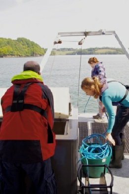
At each site the CTD rosette system was lowered through the water column to a near maximum depth and immediately recovered. Niskin bottles could be fired off remotely at desired depths to gain samples, upon recovery the samples were emptied and stored appropriately. The CTD was also fitted with a depth probe, TS probe (to measure temperature and salinity), flurometer (to measure chlorophyll fluorescence) and a transometer (to measure turbidity).
Secchi Disk:
A secchi disk was lowered over the side of the vessels through the water column until it was no longer visible. This depth is known as the secchi depth and is converted using the following equation to estimate the euphotic zone depth: euphotic zone = secchi depth (m) x 3.
Nutrients (Phosphate, Nitrate & Silicon):
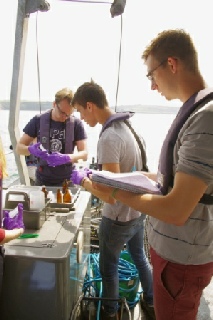
A sample was gathered from 8 stations: at sub-surface, intermediate and near bottom depths using Niskin bottles on a CTD rosette system. The storage container, syringe and pipette were all washed out with a small amount of the sample to avoid contamination that may alter the chemical signature of the samples. This sample was filtered through a 25µm porous glass fibre filter using a syringe to eliminate biological matter and particulate debris. Nitrate and phosphate samples were kept in brown bottles and stored in a dark box whilst the silicon samples were kept in plastic bottles and stored in a dark freezer. This reduced photo-degradation and stabilised the samples until they could be analysed onshore.
Dissolved Oxygen:
Two samples were collected from each station, sub-surface and near bottom. The water samples were extracted from the niskin bottle valve using a rubber tube, this reduced the samples exposure time to the atmosphere and possible gaseous alteration. The samples were kept in brown (lugol) glass bottles where a reagent solution of excess manganese (II) salt, iodide and hydroxide ions were added to the water samples, causing a precipitate to form. This precipitate was oxidised by the dissolved oxygen present, forming a second brown manganese precipitate. They were then stored in a bucket of seawater until onshore analysis.
Chlorophyll:
The samples were also gathered using the niskin bottles from the three depths. 50ml of each sample were filtered through a 25µm porous glass fibre filter using a syringe. The filter was removed from the syringe and placed into a plastic bottle containing 7ml of 90% acetone and also stored in a dark freezer.
Zooplankton
Zooplankton samples were collected at specific stations up the estuary. Samples were collected by trawling a zooplankton net behind the boat for 5 minutes, and everything caught in the net was transferred into a bottle which contained formalin.
These samples were taken to the lab and were viewed under a microscope, where each organism was identified and recorded.

Phosphate:
The procedure used was suitable at determining phosphate when in low concentrations. 1ml of a reagent was added to 10ml of each sample and allowed to stand for 1 hour. Known standard phosphate concentrations were prepared at 0, 0.07, 0.15, 0.3, 0.75 and 1.5 µmol/L. The standards were freshly prepared because when at low concentrations the solutions will decrease in concentration at an unpredictable rate within a short time period. The absorbance of the samples and standards were then measured using a spectrometer (V-180) at 882nm. The samples were then related to standards in order to correlate the absorbance to true PO4 concentrations.
Silicon:
The water samples were allowed to warm to room temperature and standards, replicates for end members, and blank samples prepared by diluting them ten fold with 5ml of MQ water. The samples were then reacted with 2ml of Molybdate Reagent for 10 minutes, resulting in the formation of three complexes; Silicomolybdate, Phosphomolybdate and Arsenomolybdate. A Mixed Reducing Reagent (3ml) was then added to the samples and left to stand for between 1.5 and 2 hrs. This decomposes the Phosphomolybdate and Arsenomolybdate whilst reducing the Silicomolybdate complex, giving a blue colouration. The absorbance of the samples, standards and blanks was then measured in a spectrophotometer (V-180) at 810nm. Like with the other nutrients, absorbance values of the standards were used to construct a calibration curve from which the true concentration of silicon can be determined.
Dissolved Oxygen Method:
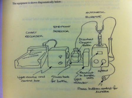
The Winkler method was applied to determine dissolved oxygen concentrations. Sulphuric acid was added to the samples, which oxidised the iodide ions into iodine. The concentration of iodine created was proportional to the concentration of dissolved oxygen present in the sample. The iodine concentration was determined using a titration reaction with thiosulphate.
A 665 Dosimat automatic burrette was used to titrate the iodine against the thiosulphate. The end point of this titration was determined by the solution colour changing from orange to clear. This change of colour was quantified by a light box and displayed on a servoscribe.
Chlorophyll:
The samples were transferred into a vial and analysed for concentrations of acetone. They were placed into a flurometer and a calculation (7/50 x flurometer value) converted the values from the flurometer reading (mg of chlorophyll /Litre of acetone) to (µg of chlorophyll /Litre of sea water.
Phytoplankton:
Phytoplankton samples were added to a solution of lugols iodine and left overnight, this allowed the lugols iodine to bind to the phytoplankton causing them to sink to the bottom of the tube. The top 90% of the solution was then siphoned off, leaving the majority of the phytoplankton. 1ml samples were pipetted out onto a Sedgewick-Rafter chamber for species identification under a microscope.
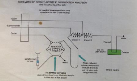
Nitrate:
The equipment was continually rinsed to stop contamination effects on results, including re-filtering. The samples once filtered and prepped were taken up by a syringe and loaded onto a system of amalgamated machines. The use of a spectrometer, a graphical printer and a peristaltic pump allowed a set volume (630µl) of sample to be tested. Adding a reagent gives colour to the samples which was recorded on the spectrometer. These were then related to standards in order to correlate the absorbance to actual nitrate concentrations.
Silicon:
Silicon behaves conservatively throughout the salinity range (Fig.4) that was sampled, although the Observed Dilution Line is slightly above the Theoretical Dilution Line (TDL). This could potentially indicate the addition of silicon further up the estuary (Head 1985) however further sampling would need to be undertaken to make any conclusions. Silicon in the lower estuary is notably higher in the surface 5m that in deeper waters, as shown at station 3 (Fig. 5). There is little association between silicon and chlorophyll.
Phosphate:
Figure 7 shows that phosphate undergoes massive addition between salinities 29 and 34. The addition could be down to runoff from agricultural fertilisers into the water , in a similar way to copper pollution from mines in the estuary(Rijstenbil et al. 1991) and without removal by biological activity, a build-up of phosphate occurs. Phosphate concentrations could be further enlarged by addition from the river tributaries that feed into the Fal Estuary.
Nitrate:
Nitrate plots below the TDL, showing that it is removed in the lower estuary between salinities 29 and 35 (Head 1985). This is due to surrounding runoff from agricultural fertilisers enriching estuarine waters with nitrate , in a similar way enrichment changes biological interactions (Addy et al. 1984) which is used up by phytoplankton blooms, shown as points below the TDL (Fig. 6). Figure 5 shows that nitrate concentration is greater in surface waters than at depth.
Physical Structure of the Estuary:
Throughout the estuary, the extent of the relationship between temperature and salinity is clearly shown by a decrease in temperature with depth corresponding with an increase in salinity. In the lower estuary, station 1 shows a well-mixed vertical profile, with stations 2, 3 and 4 showing stratification of temperature and salinity in the surface 5m, below which the water column is well-mixed (Fig. 1).
The upper estuary is characterised by a much shallower water column, with typical max depth of 12m as opposed to 30m in the lower estuary. Station 5 shows a well-mixed surface 5m, beyond which there is stratification to depth. Stations 6 and 7 appear more stratified with no bodies of well mixed water (Fig. 2). Station 8 exhibits a well-mixed water column (Fig. 3), however the station is extremely shallow, 1.2m depth, and contains relatively warmer and less saline water than the water in the lower estuary.
Differences between the upper and lower estuary may be due to the morphology of the estuary bed. A sill between stations 4 and 5 near Feock divides the shallow upper estuary and deeper lower estuary, acting as a physical barrier to incoming saline water and thus reducing tidal influence in the upper estuary. The structure of the estuary varies from well-mixed at the mouth to increasingly stratified in the shallower upper estuary, resulting in a well mixed estuary. In the upper estuary, reduced tidal influence and only one fluvial input could result in stratification even within a relatively shallow water column. However, the lower estuary acts as a basin to multiple fluvial inputs such as the Penryn River, Mylor Creek and Restronguet Creek, potentially altering the nutrient distribution.
At transect 5 (Fig. 10) two water bodies are noticeable, a laminar flowing layer (1.283) at the surface (0-4m) and a transitional layer from turbulent to laminar (0.392) at depth (8-12m) where by kinetic energy is being converted to potential energy to stabilise the water column (Mack et al, 2002). Between 4-8m a turbulent layer (0.001) indicates mixing at the interface of the two water parcels. This turbulent layer is on a small enough scale to be considered as shear instability mixing where Kelvin Helmholtz Billow mixes two water bodies t (Yang et al, 2007).The salinity and temperature profiles support this, with clear fluctuation in temperature and salinity seen in this turbulent zone characteristic of mixing.
In transect 7 (Fig. 11) a turbulent layer (0.0863) similar to transect 5 is noticeable at intermediate depths of 4-8m indicating continued mixing up the estuary. Higher current velocities from a stronger riverine input lead to growth of the turbulent zone and a less stratified thermo and halocline structure. This causes increased Kelvin Helmholtz Billow mixing at the interface of the two water bodies as a result of higher shear from the stronger velocities (Mack et al, 2002).
Laminar and Turbulent Flow of the Estuary:
The Richardson number (Ri) is a dimensionless number that expresses the ratio of potential to kinetic energy. The theory that instability and turbulence is enhanced by shear and reduced by stratification is fundamental (Zaron et al, 2008). The calculation was used to calculate the values across transects.
Where: -g = the earths gravity force (9.81m/s2), dρ= rate of change of density, dz= rate of change of depth, ρ0= average density, du= rate of change of velocity.
A spread sheet of these values was produced by combining data gathered from an ADCP and CTD. A Ri number was calculated for each depth to determine the water stability and flow type, either laminar or turbulent mixing. This helps to better understand the physical structure of the water column.
Surface Ri values are usually turbulent (close to 0) because of atmospheric influence and values close to the bed are also usually turbulent because of increased shear stress on setting mixing.
According to Richardson numbers transects 1 and 2 indicate a completely turbulent water column and consequent mixing (Fig. 8). These are the most seaward transects located at the mouth of the estuary (Black Rock). The estuary is well mixed and associated with strong tidal mixing forces which acts upon the entire water column at these transects.
Figure 9 outlines laminar flows occurring at intermediate depths (7-12m and 5-8m respectively). This indicates a slow flowing boundary layer separating the turbulent flowing freshwater (0.0023 and 0.001) and marine water (0.0014 and 0.0308). This non-mixing laminar layer prevents interaction of the water bodies and produces the seen stratified conditions.
The general trend of the lower estuary nutrients was to behave conservativly, with addition of phosphate due to agricultural runoff. Nitrate is also added by agricultural runoff but is quickly depleted by phytoplankton; lack of biological activity allows phosphate to remain in the water column.
Diatoms were the most abundant group of phytoplankton throughout the estuary. Dinoflagellates were found in the lower and upper estuary, but in some of the mid stations proportions were very small or absent. Ciliate bacteria were only found in the lower stations.
Richardson Numbers showed transects 1 and 2 were completely turbulent throughout the water column due to strong tidal forces acting upon them. Whilst transects 3 and 4 are characterised by a laminar flowing layer at an intermediate depth and turbulent flows at the atmospheric boundary and seabed. Turbulent flow is present at intermediate depths up the estuary at transects 5 and 6 once shear instability mixing becomes large due to increased riverine input. By transect 8 increased current velocities; shallower depths, atmospheric shear and seabed shear magnify the turbulent flow throughout the water column.
References:
Abarbanel. H. D., Holm D. D., Marsden. J. E. and Ratiu. T. (1984). Richardson number criterion for the nonlinear stability of 3D stratified flow. Phys. Rev. Lett., 52(1), p2352–2355.
Mack. S. A. and Schoeberlein. H. C.. (2002). Richardson Number and Ocean Mixing: Towed Chain Observations. Journal of Physical Oceanography. 34 (3), p736-757.
Scully. M., Friedrichs. C., Brubaker. J. 2005. Control of estuarine stratification and mixing by wind induced straining of the estuarine density field. Estuaries 28,3: pages 321-326.
Yang. S., Gao S. T., Wang. D. T. (2007). A study of Richardson Numbers and instability in moist saturated flow. Chinese Journal of Geophysics. 50 (2), p365-375.
Zaron. E. D. and Moum N. M. . (2008). A New Look at Richardson Number Mixing Schemes for Equatorial Ocean Modeling. Journal of Physical Oceanography. 39 (3), p2652-2664.
Zooplankton:
Zooplankton are animal members of the plankton community. These will usually feed on the phytoplankton being the most numerous primary consumer in the ocean(Vaulot 2006). Zoo plankton size can vary dramatically, and are defined by holoplankton or meroplankton(Vaulot, 2006). If an organism spends all of its life in the plankton community then they are classed holoplankton. If they only spend a portion of their life in the plankton community then they are defined as mesoplankton(Rodriguez et al., 2000).
At station 1 it appeared that copepod, copepod nauplii and decapods larva were the most abundant groups of zooplankton (Fig.13). At station 4 (Fig.14) hydromeduase was the most abundant group, with cirripede larvae and gastropod larvae being present in small abundances. Station 8 (Fig.15) had several abundant species, including copepod nauplii, cirripede larva, hydromedusa, copepoda and gastropod larvae, the abundance of zooplankton for example copepod eggs can be affected by phytoplankton(Bautista et al., 1994; Irigoien et al., 2000a).
Cirrepede larvae and gastropod larvae increases up the estuary and polychaete larvae were only found in upper estuary. However, conclusions were hard to draw due to limited sampling in the estuary and limited identification of each sample.
Chlorophyll:
The further up the estuary the greater the chlorophyll concentration, which is synonomous with increased nutrient concentrations further up the estuary (Maximum chlorophyll concentration of the lower estuary is approximately 2µg/l as opposed to maximum chlorophyll concentration in the upper estuary of approximately 10µg/l). Figure 5 is representative of all the stations, at which there is a chlorophyll maximum at 10-20m depth.
Transect 8 (Fig. 12) – The furthest upstream station in the estuary. The shallow 2m water column is entirely turbulent (0.0075 at the surface) and (0.001 between 1-2m) indicating a single fast flowing well mixed water body that is riverine dominated because of low tide. Shear stress from the atmosphere and the seabed will have a greater influence across the shallow vertical profile at shallow depths generating turbulent flow.
Phytoplankton:
Station 1 showed a large similar proportion of diatoms and dinoflagellates. a quarter of the population of station 1 was made up of one species of ciliate bacteria called Mesodinium rubrum (Fig. 16). At station 2 there was a large reduction of ciliate bacteria and dinoflagellates (Fig.17). The number of species of dinoflagellates also fell from 3 species at station 1 to 2 species at Station 2. In this station diatoms dominated especially the species Nitzschia. Diatoms were the only group present at station 3(Fig. 18), with the species Nitzschia being the most abundant. Station 3 was found to only have diatoms present. The species Nitzschia was found in the largest quantity. At station 4 (Fig.20) there were some dinoflagellates found, but like the stations before it was dominated by diatom species. At this station there was a change in the most dominant diatom species, where Coscinodiscus was in greater quantities than Nitzschia. Station 5 showed a similar dinoflagellates/ diatom ratio to station 4 (Fig.21). However the sole dinoflagellate species changed from Alexandrium to Ceratinin sp. The diatom species coscinodiscus proportion increased further from station 4 to station 5. At station 8 the proportion of dinoflagellates to diatoms remained similar to station 5(Fig.22). However the diatoms number was split mainly between 3 species which were Coscinodiscus, Guardinia flaccid and Thallasiosira.
In the Fal estuary it appeared that diatoms were the most dominant group of phytoplankton present, apart from in Station 1, down by Black Rock, where dinoflagellates and ciliate bacteria were seen in great numbers. The large diatom abundance could be explained by the Fal estuary being a temperate region, offering optimal conditions for rapid reproduction and survival of this group(Margelef 19878(Irigoien et al. 2000). The large number could also be due to the diatom spring bloom which should have been drawing to an end. At station 3 diatoms were the only group of phytoplankton found. At this station the silicon concentration was very low, which could show that the diatoms were utilising the dissolved silicon in the water (Vaulot, 2006).
It appeared that the dinoflagellates bloom had not yet occurred, as a larger number of dinoflagellates would have been expected.
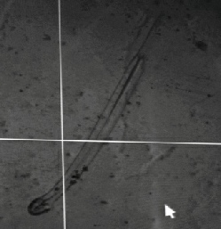
Chaetognath, commonly ‘Arrow Worm’
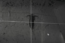
Copepod
Station 5: 50’12.463N 005’01.674
Station 8: 50’14.332N 005’00.929W