
Falmouth Group 4
23rd June- 6th July 2013
Offshore
Aims and Objectives
Data was collected in order to investigate the offshore water structure and its affect on the biological and chemical distributions, found between Lizard Point and Falmouth.
Transects were taken horizontally along and periodically crossing the front, measuring changes in temperature, salinity and fluorescence as an indicator of phytoplankton, alongside CTD drops and phytoplankton and zooplankton trawls.
For the purpose of the investigation two stations were analysed, Station 1 at 50’ 09.541N, 005’03.988W, and Station 8 at 50’00.446N, 005’01.740W.
Field Methods
An ADCP was used to establish the position of the front and determine appropriate locations for further investigation by CTD and sample collection. The maximum depth, water velocity and volume transport was all measured as a continuous transect. At each site the CTD rosette system was lowered through the water column to a near maximum depth and immediately recovered. Niskin bottles could be fired off remotely at desired depths to gain samples, upon recovery the samples were emptied and stored appropriately. The CTD was also fitted with a depth probe, TS probe (to measure temperature and salinity), flourometer (to measure chlorophyll fluorescence) and a transmissometer (to measure turbidity). Biological data was collected through the use of vertical closing plankton nets, allowing discrete zooplankton samples to be taken within the water column. At Station 8 horizontal trawls at 24m depth were taken using Bongo Nets with 200μm and 100μm nets.

References
Diehl. S., 2002. Phytoplankton, light and nutrients in a gradient of mixing depths: Theory. Ecology 83:386-393
Irigoien X, Harris R.P., Head R.N., Harbour D., (2000) ' North Atlantic oscillation and spring bloom phytoplankton compisition in the English Channel', Journal of Plankton Research 22:(12): 2367- 2371
Litt, E, Hardman-Mountford, N, Blackford, J, Jacob, G, Goodman, G, Moore, G, Cummings, D, Butenschon, M, 2010. Biological control of pCO2 at station L4 in the Western English Channel over 3 years. Journal of Plankton Research, 32 (5), 621-629.
Rodriguez F., Fernandez E., Head R.N., Harbour D.S., Bratbak G., Heldal, Harris R.P. (2000) 'Temporal variability of viruses,bacteria,phytoplankton and zooplankton in Western English Channel off Plymouth', J. Mar. biol. Ass. 80: 575-586
Southward, A.J, 1995. The importance of long time-series in understanding the variability of natural systems. Helgolander Meeresuntersuchungen, 49:, 329-333.
Widdicombe. C., Eloire. D., Harbour. D., Harris. R., Somerfield. P., 2010. Long-term phytoplankton community dynamics in the Western English Channel. Journal of plankton research, 32, 5: 643-655.
Stratification (Station 1) prevents mixing of nutrient rich water from below the thermocline, hence the lower surface nutrient concentration relative to the deep concentrations. At the thermocline small amounts of nutrients can be entrained from the deeper layer, hence why there are higher phytoplankton levels (indicated by high chlorophyll and fluorescence) at 21m. The thermocline also acts to hold the phytoplankton within the well-lit photic layer ensuring sufficient light for photosynthesis. Below the thermocline the amount of phytoplankton decreases, this is likely the result of low light levels limiting photosynthesis. At 21m depth the phytoplankton may have more chlorophyll per cell to compensate for the lower light levels; this would explain why a higher chlorophyll and fluorescence signal was observed at 21m despite having a lower individual count than the surface.
At Station 1 diatoms and dinoflagellates equally dominate the phytoplankton community, compared to stations 7 and 8 where diatoms dominate over dinoflagellates. This is because the offshore (Station 1) side of the front provides ideal conditions for dinoflagellates that thrive in the well-lit upper stratified layer (Rodriguez et al 2000 and Irigioen et al 2000). In the partially mixed waters at Station 8 diatoms dominate because they thrive in the lower light conditions caused by downward mixing. This is indicated by the more widespread vertical fluorescence profile from the CTD fig.OP3.
It was found that even though our investigation was into the summer months, where dinoflagellate blooms often define the phytoplankton communities (Margalef, 1978 (Irigioen et al., 2000)), there was still a high number of diatoms recorded at both stations. Similar results were observed by Widdicombe et al 2010 at the L4 Western Channel Observatory in June/July. He noted a second diatom bloom, dominated by smaller species of the genus Rhizosolenia and Psuedo-Nitzschia, both which appeared in high proportions at offshore Stations 1, 7 and 8. This is further evidence for the similarity between the offshore sites and the L4 station. At both stations, as expected, the vertical zooplankton distribution mirrors that of the phytoplankton, as they congregate where there are higher number of phytoplankton that provide a food source to graze on.
Overall the results from Station 1 and 8 reveal that the physical structure of the water column indirectly affects the phytoplankton communities by determining the availability of light and nutrients for phytoplankton growth (Diehl, 2002).
Under well mixed conditions (Station 8) the phytoplankton peaks at the depth where there are sufficient nutrient concentrations but also sufficient light levels for photosynthesis. However, without the limit of a strong thermocline the phytoplankton can be mixed down, resulting in a wider vertical distribution when compared to the distinct narrow peak at station 1.
At both stations the biology of the water column is reflected in the oxygen saturation, with super-saturation in the regions of higher chlorophyll reflecting net photosynthesis. Super-saturation in the surface waters is most likely the result of oxygen diffusion across the air sea boundary. Under-saturation in deeper water is a reflection of lower phytoplankton levels and therefore net respiration from autotrophs.

In order to investigate how the vertical mixing processes in the waters off Falmouth affect the structure and functional properties of phytoplankton communities, 8 stations were recorded during the offshore data collection voyage on the 1st of July 2013. To draw conclusions on the aim of the investigation, Stations 1, 7 and 8 were chosen for analysis as they display three key vertical structures, dominated by different mixing processes; at the offshore side of the front (Station 1), in stratified water (Station 7) and in partially mixed waters inshore of the front (Station 8). The other station (2 to 6) were not chosen for analysis as they display similar vertical structure to those chosen but did not contain full data sets for phytoplankton and zooplankton.
Phosphate:
The procedure used was suitable at determining phosphate when in low concentrations. 1ml of a reagent was added to 10ml of each sample and allowed to stand for 1 hour. Known standard phosphate concentrations were prepared at (0, 0.07, 0.15, 0.3, 0.75 and 1.5 µmol/L). The standards were freshly prepared because when at low concentrations the solutions will decrease in concentration at an unpredictable rate within a short time period. The absorbance of the samples and standards were then measured using a spectrometer (V-180) at 882nm. The samples were then related to standards in order to correlate the absorbance to true PO4 concentrations.
Silicon:
The water samples were allowed to warm to room temperature and standards, replicates for end members, and blank samples prepared by diluting them ten fold with 5ml of MQ water. The samples were then reacted with 2ml of Molybdate Reagent for 10 minutes, resulting in the formation of three complexes; Silicomolybdate, Phosphomolybdate and Arsenomolybdate. A Mixed Reducing Reagent (3ml) was then added to the samples and left to stand for between 1.5 and 2 hrs. This decomposes the Phosphomolybdate and Arsenomolybdate whilst reducing the Silicomolybdate complex, giving a blue colouration. The absorbance of the samples, standards and blanks was then measured in a spectrophotometer (V-180) at 810nm. Like with the other nutrients, absorbance values of the standards were used to construct a calibration curve from which the true concentration of silicon can be determined.
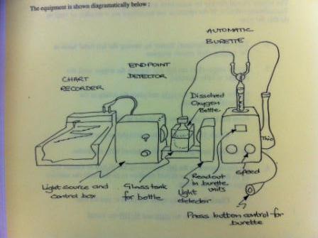
Dissolved Oxygen Method:
The Winkler method was applied to determine dissolved oxygen concentrations. Sulphuric acid was added to the samples, which oxidised the iodide ions into iodine. The concentration of iodine created was proportional to the concentration of dissolved oxygen present in the sample. The iodine concentration was determined using a titration reaction with thiosulphate.
A 665 Dosimat automatic burrette was used to titrate the iodine against the thiosulphate. The end point of this titration was determined by the solution colour changing from orange to clear. This change of colour was quantified by a light box and displayed on a servoscribe.
Chlorophyll:
The samples were transferred into a vial and analysed for concentrations of acetone. They were placed into a flurometer and a calculation (7/50 x flurometer value) converted the values from the flurometer reading (mg of chlorophyll /Litre of acetone) to (µg of chlorophyll /Litre of sea water.
Phytoplankton:
Phytoplankton samples were added to a solution of lugols iodine and left overnight, this allowed the lugols iodine to bind to the phytoplankton causing them to sink to the bottom of the tube. The top 90% of the solution was then siphoned off, leaving the majority of the phytoplankton. 1ml samples were pipetted out onto a Sedgewick-Rafter chamber for species identification under a microscope.
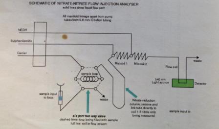
Nitrate:
The equipment was continually rinsed to stop contamination effects on results, including re-filtering. The samples once filtered and prepped were taken up by a syringe and loaded onto a system of amalgamated machines. The use of a spectrometer, a graphical printer and a peristaltic pump allowed a set volume (630µl) of sample to be tested. Adding a reagent gives colour to the samples which was recorded on the spectrometer. These were then related to standards in order to correlate the absorbance to actual nitrate concentrations.
Laboratory Methods
Station 1:
At Station 1 (Fig.OP1), a thermocline is present at 20m depth displaying a 4oC drop in temperature between the upper and lower water bodies. Turbulent flow (<0.25 Ri) is present in the surface 15m and the lower 20-47m (Fig.OR1) where the water is turbulent and in transition from laminar to turbulent. Laminar flow (>1 Ri) is seen at the thermocline along with water in the transition zone (between 0.25 and 1 Ri) moving from turbulent to laminar flow. This restricts interactions between the water parcels. These factors indicate the seaward side of the tidal front.
Nutrient concentration is lower in the surface waters, increasing with depth, Silicon peaks at 21m (~3.4ug/L) and phosphate and nitrate peak at ~46m (~3.5ug/L for nitrate, and 0.7ug/L for phosphate). A peak in fluorescence (0.21mg/m3) is seen at 20m, which is 0.13 mg/m3 higher than then average fluorescence for the rest of the water column. This peak coincides with a peak in chlorophyll a concentration at the same depth of 4.84μg/l. Fig.ON1 indicates that the water column at the surface and 20m depth is supersaturated with oxygen (107% and 101% respectively).
At 21m 4 individuals per ml was recorded, this is lower than at 1.3m depth ( 12 individuals per ml) despite the higher fluorescence and chlorophyll signals. The main species of phytoplankton observed at Station 1 were Scrippsiella (10% of sample), Nitzshia (20%), Coscinodiscus (13%) and Chaetoceros (10%) (Fig.OPhy1). Dinoflagellates and Diatoms were in roughly equal proportion at this station, (44% and 49% respectively) (Fig.) . In surface waters where the highest numbers of phytoplankton were recorded, there was also the highest number of zooplankton present with 4332 individuals per m3 of seawater. The most dominant forms of zooplankton present in a vertical sample trawled from 12m depth to the surface were Copepoda (32% of sample) and Copepoda Nauplii (11%), Gastropod larvae (16%) and Appendicularia (15%) (Fig.OZ1).
At 21m 4 individuals per ml was recorded, this is lower than at 1.3m depth ( 12 individuals per ml) despite the higher fluorescence and chlorophyll signals. The main species of phytoplankton observed at Station 1 were Scrippsiella (10% of sample), Nitzshia (20%), Coscinodiscus (13%) and Chaetoceros (10%) (Fig.OPhy1). Dinoflagellates and Diatoms were in roughly equal proportion at this station, (44% and 49% respectively) (Fig.) . In surface waters where the highest numbers of phytoplankton were recorded, there was also the highest number of zooplankton present with 4332 individuals per m3 of seawater. The most dominant forms of zooplankton present in a vertical sample trawled from 12m depth to the surface were Copepoda (32% of sample) and Copepoda Nauplii (11%), Gastropod larvae (16%) and Appendicularia (15%) (Fig.OZ1).
Station 8:
The temperature structure of the water column at Station 8 (Fig.OP3) is well mixed with maximum surface temperatures of 14.3oC and deep low temperatures at 65m of 11oC. Nutrients shows a general increase in concentration with depth, apart from a sharp decrease at ~40m, however the CTD profile does not reveal any physical structure to substantiate this decrease. Fluorescence peaks between 20-25m up to 0.20 mg/m3 with strong correlation to the chlorophyll peak of 4.84 μg/l as seen in Fig.ON3. At 0.95m the water is supersaturated with oxygen (111%), decreasing with depth but remaining supersaturated down to 45m; below this the water column because under saturated.
Surface Richardson values are closer to 0 (highly turbulent) as expected (0.1 Ri) for a partially mixed water column. The water column is structured into 4 sections (Fig.OR8): the turbulent surface layer down to 7m; the first laminar layer from 7-20m; the third section of turbulent and transitional flow, from laminar to turbulent (due to the many different water bodies present vertically, meaning less time to react and change); another laminar flow is present from 32-40m with the deep water from 45m to the sea bed in turbulent flow.

L4:
The Western Channel Observatory located in the Western English Channel provides time series measurements from two main stations, E1 (50° 02’N, 4° 22’W) and L4 (50° 15’N, 4° 13’W). For the purpose of this investigation data recorded from station L4 was compared to the data collected offshore of Falmouth to determine whether there are any similar physical, chemical and biological properties to the water mass’s, and hence, data at one point can be used to infer knowledge of the other. L4 is a fixed coastal water station situated about ~10 Km southwest of Plymouth where the water depth is 50m (Litt et al, 2010). Weekly In situ measurements have been taken from station L4 since 1988, (weather permitting), providing one of the longest time series measurements for phytoplankton. (Southward, 1995)
The phytoplankton at this station was dominated by diatoms (85%) as seen in Fig.OPhy3 with 141 individuals counted per ml with the dominant species present being Nitzshia (47% per sample), Rhizosolenia alta (13%) and Chaetoceros (19%). From the 200μm Bongo-net 205 individual zooplankton were recorded per m3 of seawater (Table.OZ) with the major species present being Copepoda (25% of sample) and Appendicularia (18%) (Fig.OB2). From the 100μm net 451 individuals were counted, (Table.OZ) also dominated by Copepoda’s (31%) and Appendicularia (30%) (Fig.OB1).
ranging between ~0.25 to ~0.6mg/m3, indicative of higher chlorophyll concentrations and subsequently phytoplankton. This could be due to an extended spring diatom bloom, early dinoflagellate summer bloom or a higher concentration of nutrients leading to greater success of the phytoplankton. Salinity over depth changes little at Station 1 between 35.14 – 35.24 and L4 data also ranges slightly between 35.05 and 35.35. The trend of decreasing salinity with depth is seen at both stations with increased change over the thermocline. The nutrient plots for 2012 (Fig.OL4b) and 2013 (Fig.OL4c) show that the L4 station has similar nutrient concentrations on a yearly basis. Due to the extremely similar physical and fluorescent properties seen at L4 and Station 1, data collected can be assumed to be a good comparison for exploring annual behaviour of nutrients and hence phytoplankton and zooplankton communities and exploring data throughout the year when sampling cannot. More time series data and vertical profiles of physical and chemical properties on the L4 station can be found at http://www.westernchannelobservatory.org.uk/
We can compare The L4 data taken on the 2nd July 2012 (Fig.OL4a) displays a strong correlation to the Station 1 Falmouth data taken on the 1st July 2013 (Fig.OP1) despite large spatial variety between the two points. This is seen by the vertical profiles in temperature, fluorescence and salinity, which follow similar trends with depth over comparable concentration ranges. The temperature ranges at L4 are seen to be between ~12.3oC and ~14.1oC compared to temperature ranges at Station 1 at ~10.7 oC to ~14.3oC. Not only are the ranges similar, but a similar thermal structure is also visible with thermoclines present at 20m (St1) and 30m (L4). There is a fluorescence maximum at both stations between the depths of 18 – 25m but L4 off Plymouth displays greater in situ concentrations


Copepod under microscope.
Personal views and information calculated on this page cannot be affiliated with the University of Southampton or the National Oceanography Centre, Southampton.
Data was collected in order to investigate the offshore water structure and its affect on the biological and chemical distributions, found between Lizard Point and Falmouth. Transects were taken horizontally along and periodically crossing the front, measuring changes in temperature, salinity and fluorescence as an indicator of phytoplankton, alongside CTD drops and phytoplankton and zooplankton trawls.
Phytoplankton growth is defined by water column structure; this is because of the circulation of nutrients. A well mixed layer means that nutrients are well distributed within the water column. This means that nutrients are not a limiting factor. The second factor influencing their growth is light. During the summer the attenuation of light is much better due to the extension of the light duration during each day. This means stratification is also important. It can be concluded that if both mixing and stratification can be achieved then phytoplankton growth would be most favoured. This occurs at frontal systems, the contrast between two water bodies on a horizontal spatial scale causes formation of a front, meaning that phytoplankton growth occurs on this boundary, with stratification aiding light attenuation and mixing supplying a constant nutrient source the phytoplankton thrive in these conditions. This can be easily seen by satellite data, where Chlorophyll a values highlight the presence of fronts based on the presence of phytoplankton.
(Satellite Data source: http://www.neodaas.ac.uk/multiview/pa/flexiview/?display_mode=wco)
Increased depths cause stratification, as surface layer mixing caused by wind is disconnected to deep water mixing as a result of tidal water body interactions, resulting in warmer upper water temperatures. As water depth decreases, the mixing caused by wind and tide converge, mixing the cooler deep water and warmer surface waters, resulting in a cooler well mixed upper water column. At the point where the upper and lower mixing layers meet, a front occurs, noted by a strong thermocline with a sharp decrease in temperature inshore of the front. It is on this very well developed thermocline that the phytoplankton flourish due to the increased nutrients and high light attenuation especially in spring and summer.