
The Fal Estuary
Date: 24/06/2013
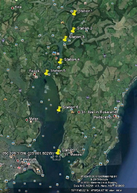
Stations:
- 1: 50◦ 14.329 N, 005◦ 0.878 W
- 2: 50◦ 13.713 N, 005◦ 0.948 W
- 3: 50◦ 13.4 N, 005◦ 1.4 W
- 4: 50◦ 12.566 N, 005◦ 1.67 W
- 5: 50◦ 12.181 N, 005◦ 2.447 W
- 6: 50◦ 10.864 N, 005◦ 1.741
- 7: 50◦ 9.135 N, 005◦ 1.802 W
Low tide: 00:50 UTC (0.3m) and 13:15 UTC (0.3m)
High tide: 06:31 UTC (5.1m) and 18:52 UTC (5.4m)
Cloud: 16%
Wind:12mph
Introduction
The Fal Estuary is a tidally dominated estuary in Falmouth, Cornwall controlled by a mixture of biological, chemical and physical processes. To test this and to see what extent it occurs 7 stations were selected along the estuary. The RV Bill Conway (photo 1) was used to take a transect ranging from the mouth of the estuary up to the most accessible inland point. A river end member sample was also obtained from much further up the river.
Materials & Methods
In the Field
The data was collected on the 24th June 2013 using a CTD (photo 2), ADCP, secchi disk (photo 3)and zooplankton net, photo 3), allowing samples of various parameters to be taken back and analysed in the lab.
At each station a vertical profile of the water column was collected by the CTD, measuring salinity and temperature against depth. Niskin bottles (photo 5) were fired at various depths at each station, typically at the lowest possible depth, halfway through the water column and at the surface and from these bottles multiple biological and chemical parameters were measured. An ADCP transect was carried out across the estuary as each station to generate a velocity cross section.
Two samples were taken of chlorophyll at each depth per station. This consisted of 50 ml of sea water being passed through a filter with a syringe. The filter was then moved to a bottle with 7ml of 90% acetone and stored in a cooler in the dark. In the lab each sample was placed in a test tube and analysed with a 10-AU fluorometer to determine chlorophyll concentration (ug/L). The fluorometer was calibrated using a blank solution of 90% acetone. The readings were adapted mathematically to account for the fact that the amount of chlorophyll in the 7ml of acetone was derived from 50 ml of water.
Samples were also taken for dissolved oxygen from within the niskin bottles using a flexible tube to minimise contaminating atmospheric oxygen. The bottle was completely filled allowing some water to flow out of the top. The samples were then fixed by adding 1 ml of Manganous chloride solution followed by 1ml of Alkaline Iodine.
Nitrogen, phosphorous and silicon were sampled from 60ml of water filtered through a syringe. A plastic bottle stored the water to be tested for silicate to prevent silica contamination from glass bottles and a brown glass bottle stored the samples to be tested for nitrogen and phosphorous.
At each station a secchi disk was lowered off the starboard stern of Conway. The depth at which the secchi disk disappeared from view was recorded and the equation k=1.4/3xsecchi depth was used to determine the light attenuation coefficient.
In the Lab
Phosphate analysis: a stock solution was diluted to concentrations between 0.07umol/L and 6umol/L. 3 replicates of each standard and blank solution were reacted with 1ml of a mixed reagent consisting of ascorbic acid and 10% potassium antimonyl tartrate. 10 ml of each sample was also reacted with the mixed reagent. Replicates were taken every 5 samples and they were left for an hour to react. A flurometer was then used to measure absorbance and a calibration curve was developed from the standards, allowing the phosphate concentration in each sample to be calculated.
Silicon Analysis: Samples were prepared using the procedure described by Mullin & Riley (Anal. Chem. Acta 12:162,1955) with the incorporation of an automated “autoanalyser” method. Each sample was reacted with molybdate solution to form silicomolbydate. The absorbance of these samples was then calculated in a spectrometer (at 810nm) using a 4cm cuvette and results were recorded. 2 sets of standard solutions as well as 3 blanks were prepared and used to create a calibration curve that was then used to determine the silicon concentrations in the rest of the samples.
Nitrate Analysis: The nitrate concentration of each sample was measured using a method developed by Morris and Riley in 1996 and later improved using flow injection by Anderson in 1979. Samples were introduced in to a flowing carrier stream using a 6-port two way valve while reagents were sequentially added with a mixing column. The pink colour that is developed from the chemical reaction is measured in a flow through 1 cm cell, held within a spectrophotometer and the signals produced are recorded on a chart. The chart recorder measures the absorbance of the samples as peaks which are then measured out in cm. An average of 3 peaks was used for each sample and 3 standards were also used.
Oxygen Analysis: The samples were stored under water to prevent further exchange of oxygen between the samples and their surroundings. 1ml of sulphuric acid was added to each sample to release the oxygen from the precipitate and a magnetic mixer was placed into the sample bottle. This was then transferred to a photospectrometer which continuously measured the light absorbance as the sample was titrated with thiosulfate. The point at which the light penetrating the sample remained constant indicated the complete removal of oxygen. The thiosulfate titre is 4 times that of the oxygen and so the oxygen content was calculated by dividing the thiosulfate titre by 4.
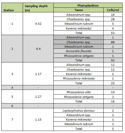
Phytoplankton Analysis: 5 phytoplankton samples were taken directly from the Niskin bottles at stations 1,2,3,5 and 7 and an iodide preservative was added. 1ml of each sample was pipetted onto a sedgewick-rafter chamber and examined under a microscope. To scale counts of individuals in the chamber to a concentration of cells/ml they were multiplied by 10.
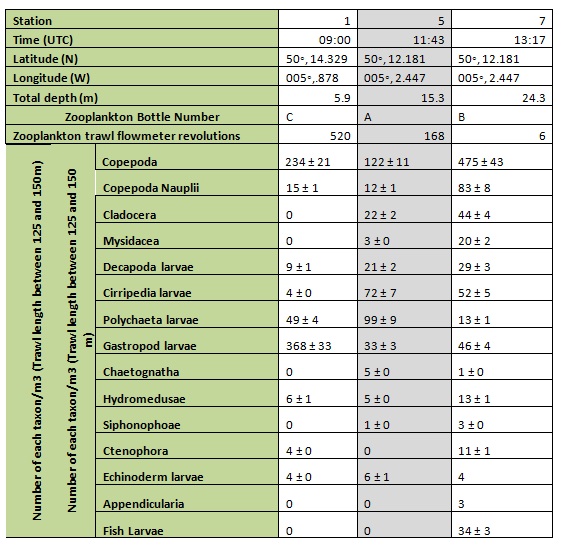
Zooplankton Analysis: At stations 1, 5 and 7 zooplankton were collected using a 200µm plankton net, samples were stored in 1 litre bottles and formaldehyde was added to preserve them. In lab the number and types of each species were manually counted and recorded. This was then multiplied to allow for the condensing of the solution. A flow meter was attached to the net to determine the flow through the net and allow an estimation of the amount of each type of zooplankton present per litre of seawater.
Results
CTD
Using the CTD data collected from the Fal estuary, temperature-salinity profiles were obtained for each of the 7 stations that were sampled along the estuary.
As can be seen fro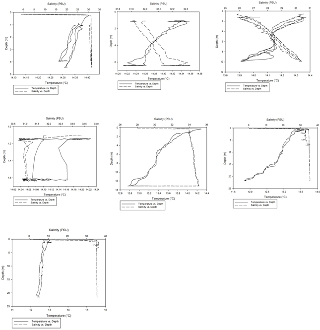 m figures 1a-g, the temperature-salinity profiles vary from station
to station. Stations 1,6 and 7 show very shallow, steep haloclines, with the salinity
increasing significantly within the first metre from the surface from around 0 up
to 32-33 and then staying fairly constant throughout the water column. Stations 2
and 3 appear to have a gradual gradient from low to high salinity from the surface
through the water column. Station 4 was extremely shallow and was only sampled down
to around 1.7 metres. The salinity decreased from 33-31 in the first 0.1 metres and
then stayed rather constant through the remainder of the water column. Finally, station
5 increased significantly from salinities around 28 up to 34 in the first 0.2 metres
and then stayed constant throughout the water column. Some measurements of salinities
around 26-28 were also recorded around 12-13 metres. From the graphs we can see that
all the stations except for 2 and 3 show steep increases in salinity within the first
0.5 metres and then remain constant whereas stations 2 and 3 show gradual gradients
of increasing salinity.
m figures 1a-g, the temperature-salinity profiles vary from station
to station. Stations 1,6 and 7 show very shallow, steep haloclines, with the salinity
increasing significantly within the first metre from the surface from around 0 up
to 32-33 and then staying fairly constant throughout the water column. Stations 2
and 3 appear to have a gradual gradient from low to high salinity from the surface
through the water column. Station 4 was extremely shallow and was only sampled down
to around 1.7 metres. The salinity decreased from 33-31 in the first 0.1 metres and
then stayed rather constant through the remainder of the water column. Finally, station
5 increased significantly from salinities around 28 up to 34 in the first 0.2 metres
and then stayed constant throughout the water column. Some measurements of salinities
around 26-28 were also recorded around 12-13 metres. From the graphs we can see that
all the stations except for 2 and 3 show steep increases in salinity within the first
0.5 metres and then remain constant whereas stations 2 and 3 show gradual gradients
of increasing salinity.
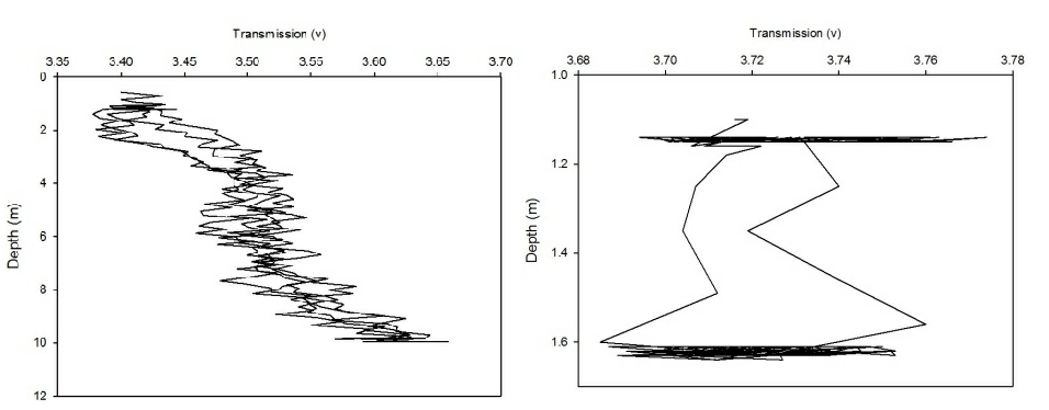
The CTD also collected data on transmission and fluorometry throughout the water column at each station. This data gives an insight into the turbidity and chlorophyll concentration. As all the calibration data has not been collected for the full two weeks, no absolute values could be obtained. Instead, the transmission and fluorometry voltage can be used as a proxy as they are relative. Figures 2(a-g) and 3(a-g) show the transmission and fluorometry profiles for stations 1-7 respectively.
The above figures show that stations 1,5,6 and 7 have high turbidity at the very surface of the water column, typically around 0.5-2 volts, which dramatically increases, within 0.1 of a metre, to around 3-4.5 volts, showing low turbidity. The turbidity then appears to remain fairly constant throughout the water column. Station 3, however, shows a gradual increase in turbidity, with a decrease in transmission from 3.3-3.5 volts to around 3.2 volts. Station 2 shows more of a gradual decrease in turbidity through the water column, increasing from around 3.4 to 3.65 volts. However, this is only a small decrease in turbidity from the surface which shows low turbidity anyway. Again, these high voltages show a general low turbidity in the water column as a whole. Station 4 also varies over a small voltage range, between 3.7 and 3.75 showing little change through the water column. Again, these relatively high voltages show a generally low turbidity in the water column.
The fluorometry-depth profiles can be used a proxy for the amount of chlorophyll throughout the water column. Figures 3a) and 3c) for stations 1 and 3 both show low voltage at the surface with an increase at 1-2m. The voltage then remains fairly constant throughout the water column. However, station 3 shows greater variation than station 1. Station 1 starts with a lower voltage than station 3 (0.15 volts as opposed to 2), but both increase to around 0.25-0.3 volts. Figure 3a) shows a peak in voltage (0.35) at around 4m and figure 3c) shows a peak in voltage (0.32) around 8m. These may indicate chlorophyll maxima. Figure b) represents station 2 and shows an extremely gradual increase from around 0.24 to 0.28 volts through the water column. However, peaks of up to 0.4v can be seen around 1, 4.5 and 6.5 metres. Station 4 (figure 3d)) was only sampled between 1 and 1.7m as it was a very shallow station. There is not much variation in this short amount of space, with voltages ranging between 0.21 and 0.23. However, a peak of 0.26 can be seen around 1.2m. Finally figures 3e-g (stations 5-7), show a similar profile to each other. The voltage remains fairly constant throughout the water column with very clear peaks at certain depths. Each station appears to show a constant voltage of around 0.2 volts throughout the water column, showing very low chlorophyll may be present. The peaks for station 5-7 can be seen at around 6, 10 and 14m respectively with the peaks ranging between 0.9 and 1 volt.
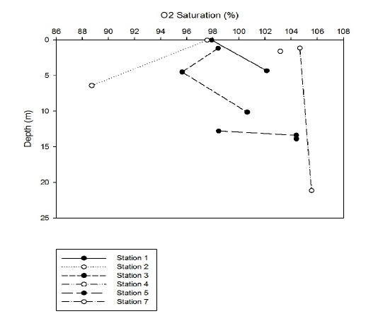
Figure 4 shows how the oxygen saturation changes through the water column at each station. Station 4 was extremely shallow and only one oxygen measurement was taken at 1.6m so is not shown on this graph. The saturation at 1.6m was 103.17%. The graph shows that, at station 1, the saturation increased from 98-102% between 0-5m. However, the oxygen saturation at station 2 decreased from 97.5 to 88% between 0 and 7m. The O2 saturation at station 3 decreased from 98 to 96 between 0 and 5m and then increased up to 100% between 5 and 10m. At station 5, the O2 saturation increased from 98 to 104% over 1m between 12.8 and 13.8m. At station 7, the O2 saturation remained fairly constant, only increasing by 2% between 1 and 22m.
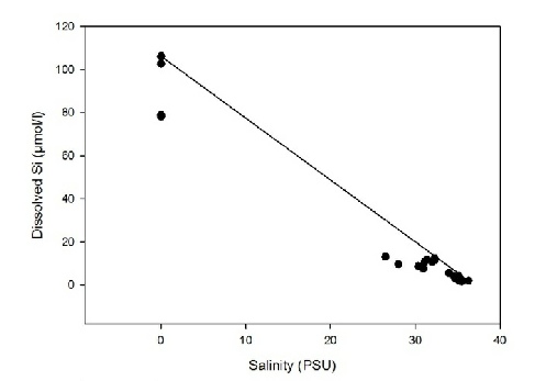
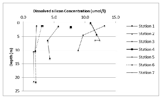
Figure 5 hows how dissolved silicon behaves along the estuary. No samples were obtained between 0 and 25 PSU so how the constituent behaves between these salinities cannot be determined. However, it would appear that between salinities of 26 and 30, a small amount of silicon is being removed from the estuary.
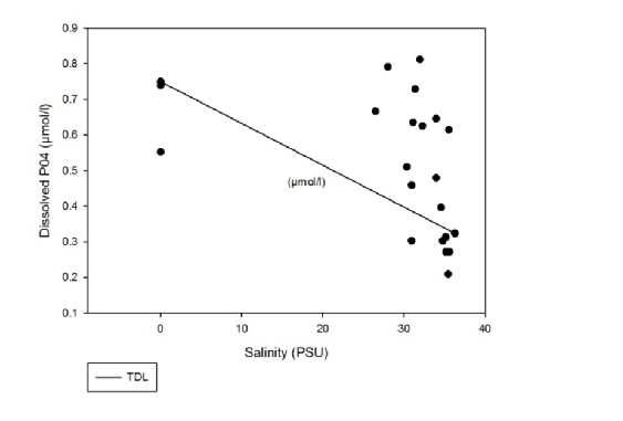
Figure 6 shows that the dissolved PO4 between salinities of 25 and 36 is acting non-conservatively. There appears to be a high amount of addition of the constituent and also some removal.
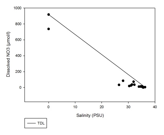
Figure 7 shows that a small amount of dissolved NO3 is being removed from the estuary between salinities of 26 and 36 and therefore is behaving non-conservatively.
Chlorophyll
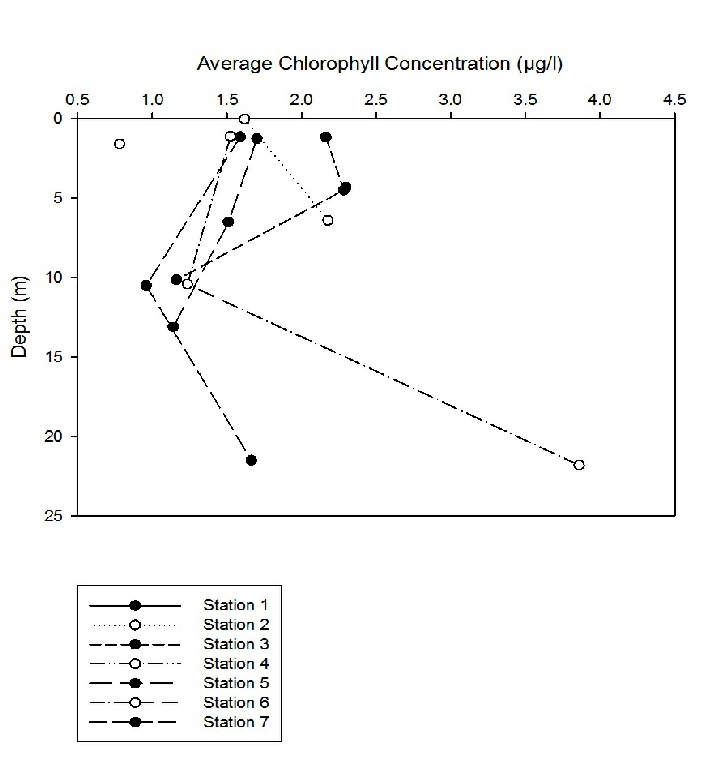
Figure 8 shows how the average chlorophyll concentration changes with depth. We can see that at station 1, the concentration increases from 1.5µg/l to 2.3µg/l between 0 and 5m. At station 2, the concentration also increases from around 1.6 to 2.1µg/l over a depth of 7m. At station 3, the chlorophyll concentration decreases from around 2.2 to 1.6 between 0 and 10m. Station 4 was only sampled at 1 depth with a concentration of 0.78. Station 5 showed a decrease in chlorophyll from 1.7µg/l to 1.1µg/l between 0 and 13m. Station 6 and 7 show similar trends, with chlorophyll concentrations decreasing and then increasing again. At station 6, the concentration decreased from 1.5 to 1.2µg/l between 1 and 10m and then increased to 3.85µg/l at 21.8m. The concentration at station 7 decreased from 1.6 to 0.9µg/l between 1 and 10m and then increased back up to 1.6µg/l at 21m.
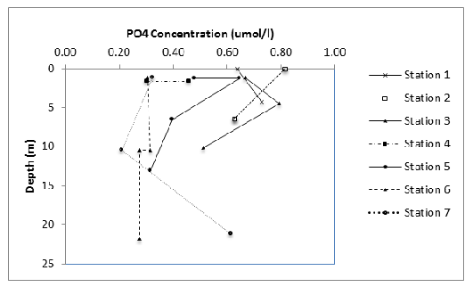
The concentration of dissolved phosphate (fig. 9) generally decreased with depth at each sampling location, apart from 1 and 3 where a slight increase was seen from the surface to approximately 5 metres and 7 where an increase was seen between 10 and 22 metres. The phosphate concentration also generally decreased with distance down the estuary with 0.8 umol/l at the surface at station compared to only 0.3 umol/l at station 6.
Nitrate concentration also generally decreases with both depth and distance down the estuary apart from at stations 2 and 3, which have a high NO3 value at the surface and at 5 metres respectively.
Silicon concentration decreases with distance downstream and with depth apart from at station 1 and 2 where a slight increase between the surface and 5 metres is seen.
Zooplankton
The total number of zooplankton (Table A) was highest at station 7 in the lower estuary with 830 individuals per m3 compared to 400 and 691m-3 at stations 5 and 1 respectively. Gastropod larvae were the dominant taxon at station 1, with copepods dominant at stations 5 and 7. The largest number of different taxa was found at station 7 with the largest number of copepod nauplii and the only fish larvae and appendicularians found there.
Discussion
The combination of all the above parameters measured at stations along the Fal estuary enables quite a detailed understanding of the behaviour of the water and constituents of the estuary.
The data taken from the CTD and plotted in transmission, fluorometer, salinity and temperature graphs appear to show a very fine surface layer of low salinity and high temperature as well as low transmission and fluorometer values, corresponding with high turbidity and low chlorophyll concentration respectively. However, this occurred for all stations and is most likely to be a result of the slightly delayed or lagged adjustment of the instruments on the CTD on entering the water from the air.
At station 1 the water column was well mixed, probably as a result of strong flow associated with the receding high tide. The constant transmission through the water column at station 1 is also indicative of well-mixed waters, though they are relatively turbid, with the lowest transmission values. A well mixed water column this far up the estuary may have been due to stronger than usual currents as a result of a spring tide with an unusually high tidal range due to the closer than usual proximity of the moon to Earth. Neap and spring cycles have a great effect on the ratio of river flow to tidal volume which tends to cause variations in mixing. An estuary that is usually partially mixed or even very stratified in neap tide can often become well mixed during a spring tide (Allen et. Al, 1980).
As sampling stations moved down the estuary, the water column became salt wedged, before again becoming well mixed and tidally dominated. A salt wedge is the most stratified type of estuary and occurs when a rapidly flowing river runs over top an area of sea water where tidal currents are weak. The less dense freshwater sits on top of the more dense salt water (NOAA). At stations 2 and 3 a salt wedge is apparent and turbidity is not uniform throughout the water column.
At station 2 there was an increase in turbidity with depth, possibly due to tidal re-suspension and flocculation at the interface of the relatively fresh river water and seawater associated with the estuarine turbidity maximum. At the tip of the salt wedge there is often a maximum of suspended particulate matter. This is due to the trapping of this matter because of a near-bottom upstream current in the region of the wedge. This occurs because of the residual gravitational circulation, the tidal velocity asymmetry and the tidal mixing asymmetry (Burchard & Baumert 1998).
At station 3, the turbidity was highest at the surface of the water, which may be due to the influx of freshwater with a high particulate load from the confluence of the Fal River with the Truro River. In river dominant estuaries there is high turbidity due to the input of SPM from land (Cleorn 1987). Downstream of station 3, turbidity steadily decreased and was constant throughout the water column at the sampling stations. This is most likely due to both low current speed at the times when we took the samples, between 11:20 and 13:17 UTC with a low tide of 0.33m above CD at 12:15 UTC, distance away from the interface of seawater and fresh water, meaning that no flocculation will take place, and to the increased depth of the water column in which the action of tidal currents to re-suspend sediment will be less dominant.
Fluorometer measurements from the CTD, which can be used as a proxy for chlorophyll concentration have a much higher resolution than do the 2 or 3 chlorophyll samples taken from discrete Niskin bottle samples at each sampling station and as such give a more detailed and accurate representation of chlorophyll in the water column, identifying the depth and intensity of peak concentrations. Both the depth and the intensity of the fluorescence (and hence chlorophyll) maxima increase with distance downstream from 4m and 0.38v at station 1 to 14m and 1.15v at station 7. This is most likely due to the increased transmission light of the water column, with lower turbidity and a smaller number of particles to scatter, allowing photosynthetically active radiation to penetrate deeper. As the water column is well mixed at the locations where the chlorophyll maximum is deepest, and as such nutrients are relatively evenly distributed throughout the water column, another variable must be affecting the depth at which the chlorophyll maximum is found.
Photosynthesis may be light inhibited at the surface and to ever increasing depths as the turbidity of the water decreases. Productivity is occasionally low near the input of sediment and increases towards the estuary mouth where turbidity decreases (Cleorn 1987). At station 4, which is only 3.4m deep, there is no clear chlorophyll maximum, perhaps as photosynthesis is light inhibited throughout the entirety of this shallow water column with relatively low turbidity.
The high number of phytoplankton found at stations 1 and 2 is most likely due to the sampling depth at these stations being in very close proximity to the observed chlorophyll maximum whilst at stations 3, 5 and 7 the samples were taken from very close to the surface, where photosynthesis may have been light inhibited and so the concentration of phytoplankton low.
The estuarine mixing diagram for nitrate, phosphate and dissolved silicon all show non-conservative behaviour. If a curved line falls below or above the straight line of an estuary mixing diagram it is either due to several water masses with different constituent concentration mixing together or to an internal source or sink. Flushing time can also cause point to fall under the straight line. (Loder & Reichard 1981) The most likely explanation in this case is that the dissolved silicon and nitrate are taken up from the estuary, due to primary production, seen here in the fluorescence maxima in the water column as well as the high numbers of phytoplankton and grazing zooplankton that they support.
There also seems to be a large addition of phosphate between the point at which the end members were taken and the point at which the estuary survey began. The potential sources of this phosphate are mine drainage sites, remineralisation from the sediment or outflow from the Newham sewage treatment works in Truro.
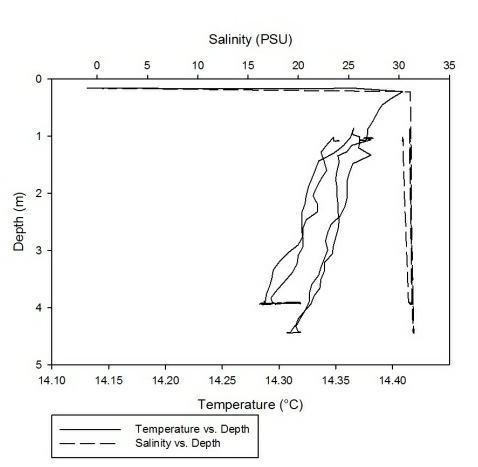
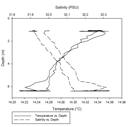
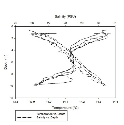
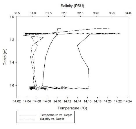
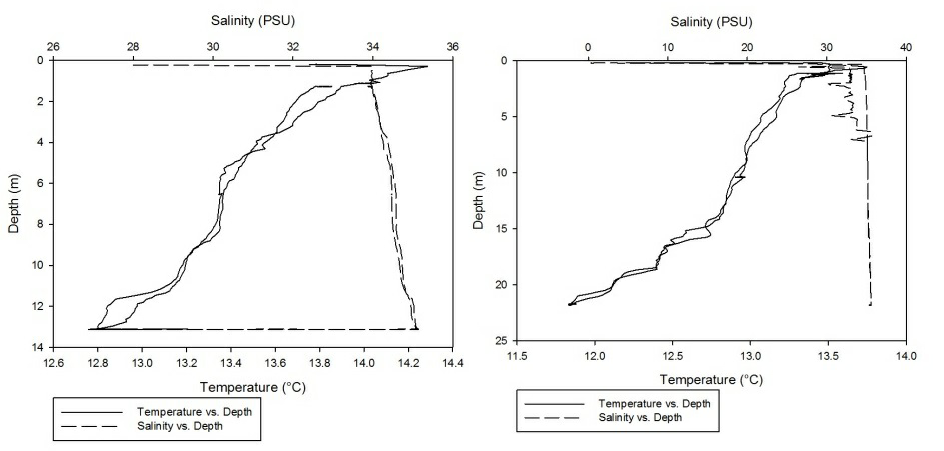
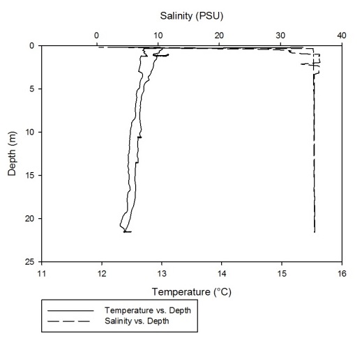
Figure 1 (A-G): Temperature-salinity profiles of the 7 stations sampled along the estuary. Figures a-g correspond to stations 1-7 respectively.
A
B
C
D
E
F
G
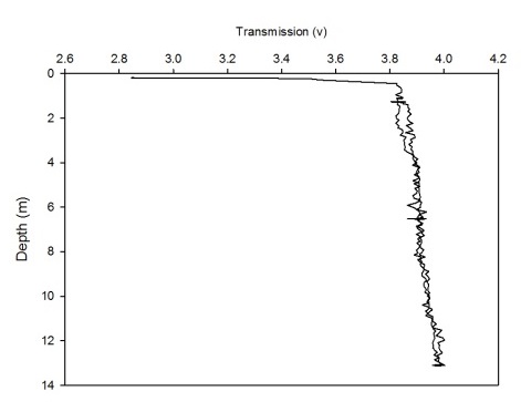
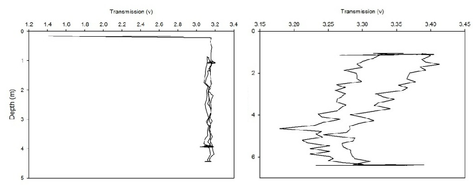
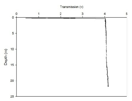
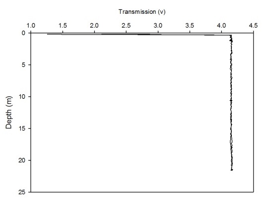
Figure 2 (A-G): Transmission-depth profiles for stations 1-7.
A
B
C
D
E
F
G
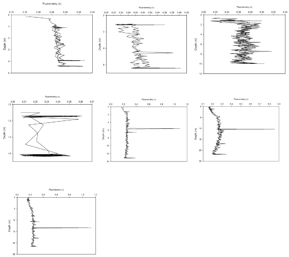
Figure 3 (A-G): Fluorometry-depth profiles for stations 1-7.
A
B
C
D
E
F
G
References
G. P. Allen, J.C. Salomon, P Bassoullet, Y. Du Penhoat, C. De granpre. (1980) ‘Effects of tides on mixing and suspended sediment transport in macrotidal estuaries’ Sedimentary Geology, vol.26 April, pp. 69-90
Burchard, H, Helmut B. (1998) ‘The Formation of Estuarine turbidity maxima due to density effects in the salt wedge: a hydrodynamic process study’, Physical Oceanography, vol.28 February, pp. 309-321
Cloern, J. (1987) ‘Turbidity as a control of phytoplankton biomass and productivity in estuaries’, Continental Shelf Research, vol.7 November-December, pp. 1367-1381
Loder T, Reichard R. (1981) ‘The dynamics of conservative mixing in estuaries’ Estuaries, vol.4, no.1 March pp. 64-69
http://oceanservice.noaa.gov/education/kits/estuaries/media/supp_estuar05a_wedge.html Date accessed 2/7/13
- AIMS: To determine how the physical, chemical and biological parameters vary along 7 stations of the Fal estuary and with depth.
- OBJECTIVES:
- To determine the salinity of water samples at varying depths of each station.
- To determine the concentrations of Si, P and N at varying depths of each station.
- To determine the temperature profiles of each station.
- To determine turbidity profiles of the water column at each station.
- To determine the fluorometry profiles of the water column at each station.
- To determine the discrete chlorophyll concentrations of water samples at varying depths at each station.
- To determine how the phytoplankton and zooplankton communities vary at different stations along the estuary.
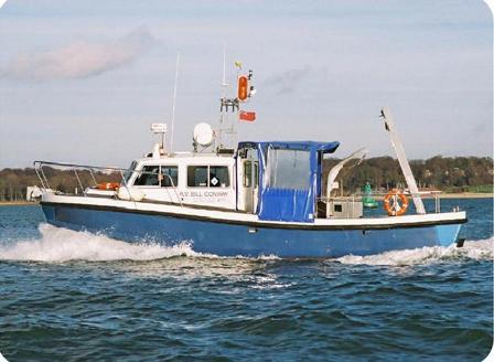
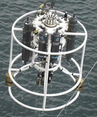
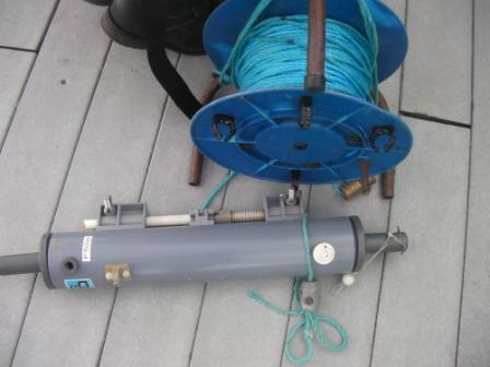
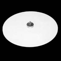
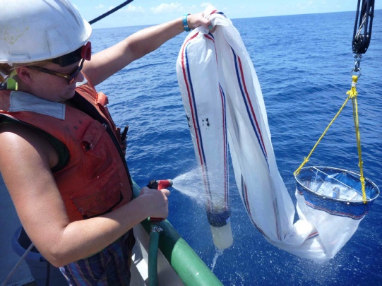
Photo 1: the RV Bill Conway
Source:http://www.soes.soton.ac.uk/teaching/courses/soes3018/2010/gr oup4/group4%20website%201%20beta.htm[Accessed 01 July 13].
Figure 4: Line graph displaying how oxygen saturation (%) changes with depth at stations 1-7.
Figure 5: Estuarine Mixing Diagram for dissolved Si with TDL.
Figure 6: Estuarine Mixing Diagram for dissolved PO4 with TDL.
Figure 7: Estuarine Mixing Diagram for dissolved NO3 with TDL.
Figure 8: Line graph showing how the average chlorophyll concentration changes with depth at each station.
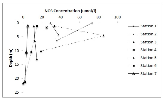
Figure 9: The change in phosphate concentration with depth and between stations.
Figure 10: The change in nitrate concentration with depth and between stations
Figure 11: The change in dissolved silicon concentration with depth and between stations
Phytoplankton
Stations 1 and 2 (Table B) show the highest number of individual phytoplankton per ml. Alexandrium and Chaetoceros are common in the upper estuary and are found at stations 1 – 3. Rhizosolenia spp. are common in the mid-estuary at stations 2-5 and the small coastal diatom Leptocylindrus is found only at station 7.
Summary
- Station 1 showed a well-mixed water column resulting from the receding spring tide.
- As collection started moving downstream a salt-wedged water column appeared before becoming well-mixed again.
- Station 3 showed a higher turbidity at the surface which may be attributed to the input of freshwater from the confluence of the Fal River with the Truro River.
- Moving downstream of station 3 turbidity decreased but was constant down through the water column.
- Depth and fluorescence increased as sampling continues downstream perhaps due to lower turbidity.
- Locations with the deepest chlorophyll maximum seem to have evenly distributed nutrients throughout the water column.
- Phytoplankton samples taken from stations 1 and 2 were taken from the depth in which there was a chlorophyll maximum while at station 3, 5, and 7 samples were taken from the surface water.
- Mixing diagrams for nitrate, phosphate, and dissolved silicon show non-conservative behaviour. Nitrate and dissolved silicon are taken up from the estuary and phosphate is added to the estuary.
Table B: Observed phytoplankton taxa and abundances in each station sample for stations 1-7.
Table A: zooplankton taxa and abundances in each station sample for stations 1-7.
Photo 2: CTD system
Source:http://teacheratsea.wordpress.co m/tag/sonar/[Accessed 01 July 13].
Photo 3: Secchi Disk
Source: http://www.fishfarming.com/services/water-soil-quality-analysis.html [Accessed 01 July 13].
Photo 4: Zooplankton Net
Source: http://www.soes.soton.ac.uk/teaching/cours es/soes3018/2009/group8/index.htm [Acce ssed 01 July 13].
Photo 5: Niskin Bottle
Source: http://www.soes.soton.ac.uk/teaching/cours es/soes3018/2009/group8/index.htm [Acce ssed 01 July 13].