
Hazel Aslin
Carlo Bella
Michael Hughes
Ben Smith
Federico Pastorelli
![]()

Sarah Lane
Clair Caldwell
Marina Brassington
Gina Selwyn
Julie Seager-Smith
![]()
![]()
![]()
![]()
![]()
![]()
Whilst in Falmouth, we have explored the length and breadth of the Falmouth Estuary, braving waves and winds offshore and mapping geophysical habitats, in order to obtain as much information as possible. The aim of the Falmouth Field Course was to investigate the Fal estuary, and offshore area in relation to biological, chemical and physical characteristics. This page gives details about the various projects that were carried out over the 12 day course including: an offshore Boat study focussed on the chemical and physical oceanic properties, with information obtained by various sampling and analytical methods. To supplement the offshore investigation, a study around the Falmouth estuary was carried out with similar investigations conducted. The geophysical habitat mapping was completed in order to determine the type of benthic habitat found in the estuary, and to observe species composition and biodiversity variations within the benthos using video data.
The Fal Estuary
The Fal Estuary is located on the English south coast and is formed from an ancient river valley that was drowned due to melting glaciers after the last Ice Age. It has subsequently formed a ria. The entrance to the estuary is located between Pendennis Point and St Anthony Head, the estuary itself extends upstream to the last point where tidal effects are felt, at Tresillian. Extensive mixing occurs within the estuary caused by tidal differences at different points along the estuary. Macrotidal conditions occur at Falmouth with a maximum spring tide of 5.3m, while mesotidal conditions occur at Truro with spring tides of 3.5m.
The estuary is divided into 2 sections with the upper estuary being fed by multiple small tributaries, forming a meandering channel. The lower estuary tidal basin, known as Carrick Roads, is wide and uniform forming 80% of the entire estuary. The total estuary length is 18km, including 127km of shoreline, and is at least 1 mile wide in all places, with a maximum depth of 34m. It represents the third largest ria estuary in the world and as well as a busy port which is important for maritime trade and tourism. It has been awarded a special area of conservation (SAC) status resulting in it having the highest levels of protection and making it important for conservation.
|
Vessel |
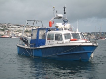
R.V. Callista |
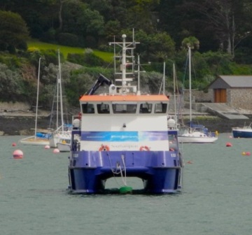
R.V. Bill Conway
|
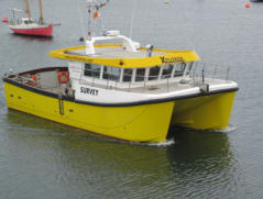
S.V. Xplorer |
|
Image |
|
|
|
|
Description |
· Length: 19.75m · Twin hulled catamaran · Used for coastal scientific studies · State of the art equipment in wet and dry labs · large rear deck for equipment (National Oceanography Centre Southampton, n.d.). · Maximum 36 passengers · Travelling range: 400 nm · Top speed 14 knots · Holds 6000 litres of fuel (University of Southampton Discover Oceanography, n.d.) |
· Designed for scientific survey work, teaching and research · Length: 11.74m · Top speed 10Kts · Maximum 12 people · Named after a former oceanography chief technician at the University of Southampton (Fisher, 2011)
|
· Class B twin engine catamaran · Owner: MTS Group · Main use: dive and survey vessel · Vessel power: 1000 horse power · Top speed 22 knots · Cruising speed 15 knots · Length: 12m Maximum capacity: 2 crew, 12 passengers.
|
|
Instrument
|
Niskin Bottles |
Acoustic Doppler Current Profiler (ADCP) |
CTD |
Rosette |
Fluorometer |
Transmissometer |
||||||||||||||||||||||||||||
|
|
|
|
|
|
|
|||||||||||||||||||||||||||||
|
Description |
- Used to collect samples for studying biological (plankton) and physical (salinity, oxygen) parameters · - Lowered on CTD with ends open · - Metal messenger released which shuts caps simultaneously · - Seals water sample in bottle at required depth. · Created in 1966 by Shale Niskin · - Update on Nansen bottles Plastic to reduce contamination |
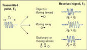
· - Measures absolute water velocity across water column · - Emits sound waves of constant frequency · Waves reflected off particles in water column · - Doppler Shift: frequency of reflected and emitted waves are different · - Waves reflected off particles moving away have a lower frequency than when emitted · - Waves reflected off particles moving toward them have a higher frequency than when emitted · - Difference between emitted and received frequency used to calculate water velocity
|
· - Conductivity, Temperature, Depth sensor · - Consists of small accurate probes · - To protect the CTD it is attached to a metal rosette · - Takes measurements as is lowered through water · - Gives real time profile of the physical water parameters · - Niskin bottles attached to the rosette to sample specific depths to corroborate sensor readings · - Attach other sensors, e.g. fluorometers, transmissometers and oxygen sensors
|
· - Metal frame · - Protects the CTD from damage - Hold multiple Niskin bottles that are pre-programmed to open at specific depths or opened remotely by sending a signal through the conducting cable connecting the rosette to the boat
|
· - Add to CTD to get vertical profile of water fluorescence · - Provides a proxy for chlorophyll and phytoplankton concentration · - Emit short wavelength light pulse (blue light) Detect longer wavelength light (red light) emitted as excess by chlorophyll after absorbing the blue light Red light emitted is proportional to chlorophyll concentration |
· - Measures light attenuation and scattering in water · - Indicates water turbidity and suspended particle concentration · - Light beam of specific wavelength passes through the water · - Transmitted light is measured · - If water turbidity is high (lots of suspended particles) there is a high absorption rate/ higher amount of scattered light thus less light is transmitted · - 100% and 0% transmissions measured to calibrate the instrument · - Done by transmitting through air (100%) and blocking off the light source (0%) - Transmission measured as a percentage of the emitted light.
|
||||||||||||||||||||||||||||
|
Instrument |
Plankton Net |
Sidescan Sonar |
Secchi Disk |
Drop Cam |
VideoRay Pro4 with HD camera |
Valeport current meter model 106 |
||||||||||||||||||||||||||||
|
|
|
|
|
|
|
|||||||||||||||||||||||||||||
|
Description |
· - Used to collect intact planktonic organisms of any size · - Towed by research vessels · - Long funnel shape · - Changing net mesh size to catch different sized plankton · - Collection cylinder (cod-end) at end of the funnel · - Various types e.g. Ring nets, Bongo nets and Multinets (Census of Marine Life, n.d.)
|
· - Used to search for and detect objects on the seafloor · - Requires 3 main components: 1. Towfish - sends and receives acoustic pulses 2. Transmission cable - attached to the towfish, sends data to the ship
3. Processing computer - used to plot data points
for visual analysis of objects or features
|
· - Created by Pietro Angelo Secchi SJ in 1865 · - Circular disk used to measure water transparency · - Mounted on a pole or line · - Lowered into water · - When pattern on disk is no longer seen, depth is recorded and taken as a measure of water transparency · - Known as the Secchi depth · - Related to water turbidity. (Sancaktar, 2009)
|
· - Used to record seafloor · - Used to ground truth side scan data - Provides video data that can corroborate sediment type
|
· - Used for education and exploration · - Operated by Natural History Museum London and University of Southampton · - Includes internal advanced navigation systems and high efficiency horizontal thrusters · - Maximum manoeuvrability, quick responses to controls, excellent thrust to weight ratio · - 2 cameras - main camera looks forward, secondary camera can be positioned in a location to suit needs · - Each camera tilts 180°, second camera pans 360° providing unrivalled video coverage |
- Used to measure the speed of a current - Measures speed of the current using a high impact styrene impeller. - Roughly 125mm in diameter with a 270mm pitch - Can record velocities from 0.03m/s to 5m/s - Has an accuracy of ±1.5% or reading above 0.15m/s. and ±0.004 m/s below 0.15m/s - Measurese direction off the flow using a flux gate compass - Mesurse in the range 0° to 360° - Has an accuracy of ±0.20
|
||||||||||||||||||||||||||||
|
Instument |
Li-cor light meter |
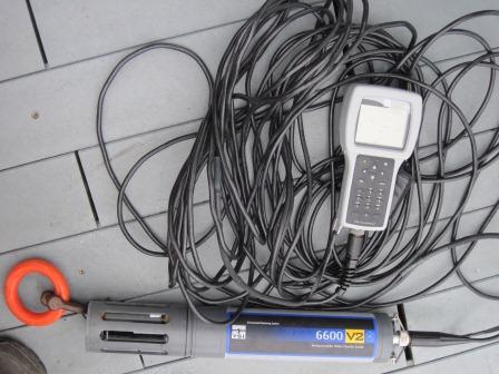
YSI multi Probe |
||||||||||||||||||||||||||||||||
|
|
|
|||||||||||||||||||||||||||||||||
|
Description |
- Li- - li-cor light meter can be lowered through the water column by hand or winch. - - Measurements displayed on a digital output; the li-cor 1400. - Multiple light measurements made simultaneously; terrestrial and marine measurements made at the same time and displayed instantaneously. |
-
|
||||||||||||||||||||||||||||||||
![]()
Introduction:
|
Date: 26/6/12 |
Instruments used: |
|
|
Vessel: RV Callista |
ADCP, CTD rosette, Niskin bottles, ROV, |
|
|
Departure: 08.20 GMT |
Secchi disk, Fluorometer, Transmissometer, |
|
|
High water: 09.22 GMT: 4.50m |
Phytoplankton net (link to descriptions) |
|
|
Low water: 15.52 GMT: 1.20m |
Heading: 180°C |
Crew: 17 |
Data was collected from four stations along a 180° bearing at 5 nautical mile intervals in order to investigate the water column structure as we moved progressively offshore into deeper open water. Figs. show our track and each station
Aim:
Investigate how vertical mixing processes in the waters off Falmouth affect, directly and indirectly, the structure and functional properties of plankton communities.
|
Station |
Lat |
Long |
Weather Conditions |
|
1 (Black Rock) |
50 08.858N |
005 01.522W |
100% cloud cover, 3mph SW wind |
|
2 (Manacle Point) |
50 04.091N |
005 00.896W |
100% cloud cover, light rain, 2mph W wind |
|
3 (Black Head) |
49 59.156N |
005 01.528W |
50% cloud cover, 3mph SW wind |
|
4 (Lizard Point) |
49 54.745N |
005 01.232W |
50% cloud cover, 3mph SW wind |
|
Planktonic Group |
Station |
Depth (m) |
Time (GMT) |
|
Phytoplankton |
3 |
10-11 |
13:05 |
|
4 |
10-11 |
14:40-14:45 |
|
|
Zooplankton |
1 |
15-6 |
08:20-08:25 |
|
2 |
25-10 |
10:45-11:00 |
|
|
3 |
20-5 |
12:10-12:20 |
|
|
4 |
25-10 |
14:30 |
Method:
Sampling
The ADCP was recording data continuously to measure the velocity and direction of flow beneath the vessel. At each station, a CTD was deployed, carrying a rosette system with six Niskin bottles. A transmissometer and a fluorometer were also attached to the system. These instruments were used to provide information about the characteristics and stratification of the water mass at different stations and allow for comparisons between each. The Niskin bottles were used to capture a sample of water from selected depths depending on the characteristics or interesting observations that were seen on the CTD profile such as a chlorophyll peak. Zooplankton were collected in a net, which was deployed from the stern of Callista, with weights attached to the bottom of the net to pull it down to the required depth, with the aid of a winch system and an A-frame. Messengers (brass weights) were sent down the line to close the net at the required depth, trapping zooplankton to indicate the composition at discrete points in the water column. The net was then recovered onto deck and washed with a hose to ensure all of the zooplankton were collected in the bottle at the “cod end” of the net. A secchi disk was deployed at each station. At the point in which the pattern on the disk was no longer seen the measurement of the depth was recorded as observed SD depth, this was taken as the measurement of the transparency of the water. Phytoplankton samples were attained discretely using the ROV at specific depths and collected in plastic bottles, into which Lugol was added to preserve the sample. 10ml samples were used in the lab, which were analysed under a light microscope.
Analytical
Silicon, Phosphate and Chlorophyll:
Carried out as per Parsons et al. 1984.
Nitrate:
Flow injection method as per Johnson, K et al. 1983.
Dissolved Oxygen:
Carried out as per Grasshoff, K et al. 1999.
Results:
Vertical profiles:
Station 1: Black Rock (fig. 3 )
Dissolved oxygen decreases with depth from 103.00% at 6.70m, to 98.80% at 26.00m. Chlorophyll was recorded at a concentration of 2.21mg/l. Salinity is highly variable within the surface meter before stabilising at 1.20m to 35.10, the salinity then increases at a steady rate to 35.24 at 26.72m. Fluorescence levels steadily increase with depth from the measurement closest to the surface, having a value of 0.02mg/m3 to 16.13mg/m3 at 5.00m. Recorded values then fluctuate between 5.00m and 26.69m throughout the section of the water column sampled. Temperature decreases from the measurement closest to the surface, with a temperature of 13.75°C to 12.54°C at 26.62m. Data for silicon, nitrate and phosphate concentrations were not collected at this station.
Station 2: Manacle Point (fig. 4)
Dissolved oxygen decreases from 101.30% at 16.50m, to 95.50% at 39.20m. Temperature decreases from 13.09°C at the surface to 12.40°C at 54.06m. Salinity remains fairly constant in the first 25.05m at 35.30, but then there is a slight increase between 25.00m and 29.00m where salinity increases to 35.40 representing a small halocline. Fluorescence decreases from the measurement closest to the surface at 0.07mg/m3, and then fluctuates between 5.00m to 30.00m between 0.10 - 0.11mg/m3. It then decreases to 0.08mg/m3 between 30.00m down to 54.06m to. Silicon decreases from 0.44µm/l at 16.50 meters, to 0.42µm/l at 39.20m. Nitrate has a concentration of 0.80μm/l at a depth of 39.20m. Phosphate concentration increases with depth, from a concentration of 0.39μm/l at 16.50m, to a concentration of 0.41μm/l at 39.20m. Chlorophyll concentration also increases with depth, with a value of 0.47mg/l at 16.50m, and a higher value of 1.90mg/l at 39.20m.
Station 3: Black Head (fig. 5)
Temperature decreases with depth, with the highest temperature recorded at 14.23°C at the surface, to 12.51°C at a depth of 66.28m. It decreases steadily from just below the surface at 0.64m, to a temperature of 12.66°C at 12.21 meters where it slopes off becoming almost constant to the bottom of the profile. Salinity is variable in the surface waters ranging between 33.02 and 35.90. It remains at a constant level through the rest of the water column that was sampled. Fluorescence increases from 0.07mg/m3 at the surface, to a peak of 0.24mg/m3 at 9.30m, it then decreases to between 0.09mg/m3 at 20.17m after which it remains constant through the rest of the profile. Silicon decreases with depth, with a concentration of 0.46µm/l at 1.80m to a concentration of 0.44µm/l at 45.60m. Nitrate levels decrease, from 4.70µg/l at 11.39m, to a concentration of 0.96µm/l at a depth of 45.60m. Dissolved oxygen percentage also decreases with depth, from a percentage of 114.30% at 1.8m, to 107.50% at 11.40m, and then decreases again to a percentage of 101.40 at 45.60m. Phosphate concentrations show an increase from the measurement at the surface showing 0.23µg/l at 1.80m, then increasing to a concentration of 0.23µg/l at 11.39m, and a decrease to 0.22µg/l at a depth of 45.60m. Chlorophyll increases with depth from the measurement made closest to the surface at 1.80m of 0.2215mg/l, increasing to a concentration of 5.64 mg/l at a depth of 11.39 meters, before decreasing to a concentration of 1.05mg/l at a depth of 45.46m.
Station 4: Lizard Point (fig. 6)
Temperature decreases rapidly with depth, from 14.75°C at a depth of 0.07m, to 13.18°C at 20.26m, then decreasing at a steadier rate to 12.50°C at 26.47m, showing the presence of a thermocline. Temperature remains fairly constant down to 69.05m at values around 12.40°C. Salinity is variable in the surface waters down to 1.00m, and then remains constant around 35.30 from 1.30m down to 69.80m. Fluorescence increases from 0.03mg/m3 at the surface to 0.20mg/m3 at 20.95m. It then decreases to 0.06mg/m3 at 26.47m where the value remains fairly stable down to 69.05m. Silicon decreases with depth from 0.48µg/l at 1.80m to 0.47µg/l at 49.89m. Nitrate is at a concentration of 1.10µg/l at 1.83m. Dissolved oxygen decreases from 112.10% at 1.82m to 102.90% at 21.87m, it then increases to 106.5 % at a depth of 49.89m. Phosphate decreases with depth, with a value of 0.17µg/l at 1.80meters to 0.33µg/l at 49.89m. Chlorophyll increases from 1.86mg/l at 1.82m, to 7.70mg/l at 21.87m, and then decreases to 0.90mg/l at 49.89m.
Biological:
|
Zooplankton |
||||
|
|
Cells/l |
|
|
|
|
Taxa |
Station 1 |
Station 2 |
Station 3 |
Station 4 |
|
Copepoda |
3800 |
7200 |
4500 |
9300 |
|
Copepoda nauplii |
2700 |
200 |
0 |
3400 |
|
Decapoda larvae |
600 |
1300 |
1000 |
700 |
|
Chaetognatha |
100 |
1000 |
100 |
200 |
|
Echinodermata larvae |
100 |
0 |
0 |
200 |
|
Appendicularia |
1300 |
100 |
0 |
1200 |
|
Cirripedia larvae |
100 |
600 |
100 |
1600 |
|
Polychaeate larvae |
300 |
300 |
400 |
300 |
|
Gastropod larvae |
200 |
300 |
0 |
500 |
|
Hydromedusae |
1000 |
300 |
300 |
500 |
|
Fish larvae |
0 |
100 |
0 |
0 |
|
Cladocera |
0 |
0 |
0 |
200 |
|
Total |
10200 |
11400 |
6400 |
18100 |
|
Phytoplankton |
||||
|
Station 3 |
|
Station 4 |
|
|
|
Species |
Tally |
Cells/ml |
Tally |
Cells/ml |
|
Alexandrium spp. |
0 |
0 |
2 |
20 |
|
Ceratium fusus |
1 |
10 |
0 |
0 |
|
Chaetoceros spp. |
5 |
50 |
1 |
10 |
|
Coscinodiscus spp. |
1 |
10 |
10 |
100 |
|
Guinardia flaccida |
0 |
0 |
1 |
10 |
|
Guinordia delicatula |
2 |
20 |
2 |
20 |
|
Karenia mikimotoi |
1 |
10 |
1 |
10 |
|
Leptocylindrus danicus |
0 |
0 |
1 |
10 |
|
Rhizosolenia alata |
0 |
0 |
1 |
10 |
|
Rhizosolenia imbriata |
0 |
0 |
1 |
10 |
|
Scrippsiella spp. |
0 |
0 |
1 |
10 |
|
Total |
|
100 |
|
210 |
Physical:
ADCP:
Station 1: Black Rock (fig. 7)
The ADCP data at station 1 shows a decrease in backscatter with depth. The backscatter ranges from around 80 to 90dB in the top 3m then decreases gradually down to 70dB at a depth 25m. The highest recorded backscatter was 188dB, 45mins in to the recording and at a depth of 3.58m. The velocity of the water column ranged between 0.02m/s to 0.08m/s during the time of the recording. There was a peak in velocity 41mins into the recording of 0.5m/s at 2.58m. The flow direction was drastically variable with no consistent direction. The vessel drifted about 140m around the start point and then headed south.
Station 2: Manacle Point (fig. 8)
The ADCP data showed that there was a larger amount of backscatter in the top 3m of the transect at around 110dB. The backscatter then gradually decreased through the water column uniformly along the transect decreasing to around 70db at a depth of 55m. The velocity of the water column gradually changed along the transect from around 0.4 m/s to 0.2m/s consistently throughout the water column. The flow direction was northward throughout the water column along the transect. The ship drifted in a fairly linear motion 1000m north from the start point.
Station 3: Black Head (fig. 9)
At station 3 the ADCP data shows that there was higher levels of backscatter in the upper 25m of the water column of around 80dB. The surface waters had the highest levels of backscatter recorded with the highest recorded 7.50mins in to the transect at over 100dB. The velocity of the water column increased throughout the transect from 0.03m/s up to 0.10m/s in the first 48mins. The last 45 minutes of the transect saw the velocity increase from 0.10m/s up to and over 0.50m/s. The highest velocity was at 53.39m 80mins into the recoding at this station. There was a large change in the flow direction throughout the water column, changing from around 70-80° in the first 10 minutes to 200° after 45mins. The flow then stayed at around 200° for the remainder of the recording time.
Station 4: Lizard Point (fig. 10)
Station 4 showed a consistent band of backscatter measuring around 80dB at a depth range of 10m to 30m. From below 30m the backscatter remians lower at 70 dB. The highest backscatter recorded was 109dB occuring in the first 9mins at a depth of 3.59m. The backscatter is highest in the first 1-3m along the transect time. The flow velocity is highest between 20m and 40m during the recording time with a velocity magnitude of between 0.40m/s to 0.53m/s. The velocity was slightly slower in the top 20m ranging from 0.15m/s to 0.30 m/s. The flow direction was largely uniform throughout the water column and during the recording time with a direction of 240°. The ship drifted about 500m in total above and below the start point.
Richardson's Number:
The Richardson number is used to establish the balance between the stabilising effect of the density gradient and the destabilising effect of the current sheer.
The Richardson number uses, the effect of gravity, the changes in density through the water column, the depth of the water column and the velocity. The requirements for the Richardson number are provided by a combination of the CTD and the ADCP. Where the CTD is used to obtain the density profile and the ADCP is used to obtain the depth of the water column and the velocity throughout the water column. For these calculations the Richardson number has been derived for the water column as a whole. Whereby the densities are taken from the top and bottom of the water column using the CTD, while the velocity is an average of the water column obtained from the ADCP.
The Richardson number can be divided into three parts whereby;
If Ri <0 = gravitationally unstable, overturning occurs
If 0<Ri<0.25 = shear flow instability develops
If Ri>1= the flow is stable and no mixing occurs between the layers.

g = Gravity
p = density
z = depth
U = velocity
Station 1
Station 1 shows a variable Ri through the water column. In the top 10 meters there is an Ri of 15.51 which then steeply changes to 256.26 between 10 to 20 meters deep. Between 20 to 30 meters deep the Ri decreases to 0.4. Between 0 to 20 meters the Ri stays above 1 indicating that it is unlikely there is mixing between the layers. At 20 to 30 meters the Ri of 0.4 means that there could or could not be mixing between the layers.
Station 2
Station 2 shows that between 5 to 15 meters there is a Ri of 0.19, as this is below 0.25 it would suggest a likehood of mixing between the layers unlike from 15 to 45 m deep where the Ri is above 1 which would suggest mixing between the layers is unlikely.
Station 3
Station 3 suggests that from 1 to 30 meters there is no mixing between the layers with an Ri of 1.28 between 1 to 10 meters deep and an Ri of 2.12 between 20 to 30 meters deep. At 40 to 50 meters deep there is an Ri value of 0.38 this suggests that there may or may not be mixing between the layers.
Station 4
Station 4 has Ri numbers above 1 throughout the water column, this would suggest that there is little mixing between the layers especially from 20 to 35 meters deep with an Ri of 135.5. At 40 to 55 meters there is a low Ri of 1.27 however this means that there is only a low chance that mixing is not occurring.
Light:
|
Station |
Observed SD Depth (m) |
Approx Euphotic Zone Depth (m) (3 x SD depth) |
Attenuation Coefficient (k) (K = 1.44/Observed SD Depth) (m-1) |
1% SD light depth (m) (z = {ln(Eo) – ln(Ez)}/k) |
|
1 |
7.5 |
22.5 |
0.192 |
23.985 |
|
2 |
8 |
24 |
0.18 |
25.584 |
|
3 |
7 |
21 |
0.206 |
22.355 |
|
4 |
7 |
21 |
0.206 |
22.355 |
To calculate the Euphotic zone depth: Euphotic zone Depth = observed SD depth x 3
Attenuation Coefficient = k
K = 1.44/Observed SD depth
1% light depth: z = {ln(Eo) – ln(Ez)}/k
Discussion:
Tidal fronts are formed in shallow seas where there is sloping bathymetry and strong tidal currents, for example, the Western English Channel (Pingree and Griffiths, 1978). Furthermore Frontal regions have a shallow pycnocline which results in the upwelling of nutrient rich water from the deep (Heilmann et al., 1994).
Profiles:
At station 1 salinity and temperature decrease only slightly throughout the water column therefore it is well mixed (Fig. 3). A gradual temperature gradient extends from the surface to 14.70m where a weak thermocline is present. Salinity shows an isohaline profile throughout the whole water column with a salinity spike of 35.41 at 1.08m which is probably due to the rapid change in temperature in the initial part of the water column or CTD lags. The water column structure is confirmed by the ADCP data, which show a homogenous water column with a single water mass (Fig. 7). Furthermore this could be the result of strong tidal mixing and wave action as station 1 was the closest to the shore. Fluorescence, which is a proxy for chlorophyll indicating phytoplankton concentration, peaks at 4.84m depth with a concentration of 0.16mg/m3 which is therefore the chlorophyll maxima of station 1. However fluorescence has a very small range, 0.16mg/m3 to 0.08mg/m3 and it is highly variable throughout the water column showing no clear overall trend. This indicates that phytoplankton cells are distributed over the whole water column and it is confirmed by the ADCP data as the backscatter is relatively high for the whole water column, but particularly within the first 10m where it reaches values of 90dB. The depth of euphotic zone worked out from the Secchi disk is of 22.50m, which is near to the bottom at the water column therefore, phytoplankton cells are able to receive sufficient light for photosynthesis, this could be why fluorescence and therefore chlorophyll values are relatively high throughout the entire water column. This cannot however be established as there were no phytoplankton samples collected at this station. The percentage of dissolved oxygen decreases with depth and ranges between 103.00% and 98.80%, this small range could be due to the well mixed nature of the water column. This cannot be confirmed as only 2 values are available. Similarly, only one value is available for chlorophyll therefore no significant trend can be observed.
Station 2 shows a gradual temperature gradient throughout the water column without any clear thermocline while salinity is homogenous apart for a small halocline at 25.1m (Fig. 4). This is confirmed by the ADCP data (Fig. 8) and it is possible to say that the water column at station 2 is slightly more stratified than at station 1. In fact station 2 is further from the shore than station 1 therefore less subject to tidal mixing which in a coastal system is the one of the major factors responsible for the mixing of the water column (Garrett et al. 1978). A salinity spike of 35.75 is present at 0.69m which is due to the reasons discussed above. Fluorescence has a small overall range, but it varies a lot through the water column which is similar to station 1 with the highest peak of 0.12mg/m3 at 15.88m indicating a chlorophyll maxima. However it is possible to observe an overall trend which shows fluorescence increasing from 0.13m to 15.88m and then decreasing to 54.06m. Moreover the depth of the euphotic zone calculated from the Secchi disc is 24m, this is why most of the fluorescence indicating phytoplankton is found above this depth. However there is fluorescence below the euphotic zone, this could be due to turbulence or the fact that certain species of phytoplankton, mainly dinoflagellates, are motile. These species are able to migrate vertically in order to receive sufficient light and benefit from nutrients (Ross and Sharples, 2007). However, this cannot be confirmed as no phytoplankton samples were collected from station 2. The percentage of dissolved oxygen decreases from the zone of highest fluorescence to the zone of lower fluorescence, this does not support the data as, in the presence of high phytoplankton concentration the percentage of dissolved oxygen should be lower due to it being respired by the phytoplankton present. As only two measurements are available for this parameter it is not possible to perform a precise analysis. The same is true for the nutrients silicon and nitrate as only 2 values are available. However silicon does appear to decrease from the zone of highest fluorescence to a zone of lower fluorescence which could be due to the presence of diatoms which use silicon in large amounts to produce their hard mineral fustule composed of silicic acid (Miller, 2004). The opposite is true for phosphate which could again be due to the phytoplankton species present within the water column, dinoflagellates are able to survive under low phosphate concentrations. Only one value of 0.8µm/L was collected for nitrate and being very low it could be considered that a high phytoplankton concentration may be responsible for example diatoms use nitrate in large amounts.
Station 3 shows a more pronounced stratification with a thermocline being present from the surface to 12.21m where the temperature decreases by 1.72°C. Salinity is instead constant with depth, showing an isohaline profile, apart from a large salinity spike at the surface and a very small halocline at 10m (Fig. 5). The ADCP data confirms this as it is possible to distinguish two different water masses (Fig. 9). Fluorescence variation is very distinct, with a pronounced peak at 9.29m which coincides with the highest chlorophyll value of 5.64µM/L at 11.39m indicating chlorophyll maxima and that most phytoplankton are present in this area. The depth of the euphotic zone calculated from the Secchi disc depth is 21m which is where fluorescence values are low and start to be constant down the water column. For this reason the phytoplankton were sampled from 10m depth using a syringe mounted on an ROV. Silicon and dissolved oxygen decrease from the surface, where they are present in their highest concentrations, to depth while nitrate and phosphate peak at 11.39m where most of the phytoplankton is found. However values for all the nutrients are very low indicating that they have been depleted by phytoplankton.
Station 4 shows a thermocline beginning at 0.06m and ending at 20m while salinity is very constant throughout the column representing an isohaline profile (Fig. 6). Two different water masses can be seen from the ADCP data. Furthermore there is a lot of backscatter especially at the surface which could be indicative of a front (Fig. 10). Moreover, the direction of the flow is mainly around 178° which could indicate vertical movement of water. Fluorescence shows a very pronounced chlorophyll maxima at 20.95m which coincides with the maximum values recorded for chlorophyll of 7.74µM/L at 21.87m depth. Moreover the depth of the euphotic zone worked out from the Secchi disc depth is 21m which agrees with the fluorescence and chlorophyll data indicating that most of the phytoplankton are found above 21m. Dissolved oxygen is lowest at 21.87m which coincides with the highest chlorophyll values indicating again a high concentration of phytoplankton. Silicon decreases with depth which could be due to the presence of diatoms while the opposite is true for phosphate which is present in higher values below the euphotic zone where it will be utilised less due to the low abundance of phytoplankton. Only one value was recorded for nitrate which does not allow a precise analysis. The position of the chlorophyll maxima confirm the hypothesis of the presence of a front at this station which is at 30m, in fact phytoplankton is normally found just above fronts where it can benefit of nutrients bought up by cold upwelling waters.
Biology:
Phytoplankton (fig 12)
The dominance of diatoms over dinoflagellates shown in figure 14 is not representative of the expected cycle of seasonal succession in phytoplankton (Margelef, 1958), whereby diatoms bloom in spring, around April-May due to their ability to compete in low temperature and light levels, provided nutrients are high. This generally results in silica depletion as it is incorporated into opal tests (Holligan and Harbour, 1977). There is subsequently a decline in the proportion of diatoms by the summer months, including July; the time at which these samples were collected. This is usually accompanied by a rise in the proportion of dinoflagellates, which, unlike diatoms have cellulose armour plating, so are not affected by the depletion of dissolved silicon and are able to compete well in these conditions. This deviation from the expected abundance could be explained by the close proximity of sample sites to the shore; station 4 was the furthest station but was still only 6.54 nautical miles out to sea. This region may have been enriched with nutrients from terrestrial origin which reach the coast via the Helford River and River Fal, which would have had an enhanced flux in mid and late June due to particularly heavy rainfall. A possible result of this is an extended spring bloom, which may even have been delayed in the first place by enhanced mixing or lower than usual temperatures. Furthermore, the energy from the wind which accompanied the heavy rain may have resulted in mixing, preventing the seasonal stratification which would otherwise give a competitive advantage to dinoflagellates (Barlow, 1980).
This hypothesis is supported by the data, which shows a large spike in chlorophyll levels for stations 3 and 4, whereby levels peak at 11.39m (5.64µm/l) and 21.87m (7.74µm/l) respectively. This spike indicates the chlorophyll maximum in the euphotic zone. (Fig 5 & 6) shows that chlorophyll concentrations are inversely proportional to dissolved silicon down to the chlorophyll maximum, past which it is no longer utilised. At station 3, the total cell count was found to be 100/ml; 48% of the count found at station 4 (210/ml). This correlates with the nutrient level data, which shows that station 3 had lower silicate than station 4, but more nitrate which suggests it had been utilised to a lesser extent by phytoplankton. Station 4 has a higher concentration of phosphate, although this is needed to a much lesser extent than nitrogen, in accordance to the Redfield ratio of 16:1. The data suggests that the diatoms are at highest density near the thermocline. The increased species diversity seen at station 4 may be a result of reduced dominance by individual species. Phytoplankton distribution is controlled by water turbulence, which is in turn a function of the hydrodynamic regime and stratification. This is influenced by the position of a point in relation to a frontal system, which effects the species composition and therefore community structure. It was found in studies by Heilmann et al. (1994), that the less stratified side of the front with less stability has more mixing and therefore more productivity. The same study also showed phytoplankton were found in higher abundance around fronts than in surrounding areas.
Zooplankton (fig 13)
Zooplankton was dominated completely by copepods and their nauplii, together comprising 77% and 70% of composition for stations 3 and 4 respectively. There was not a homogenous distribution of zooplankton throughout the entire study area; it was found in the highest abundance at station 4, also the site at which their food source of phytoplankton was greatest. This is an expected pattern in their distribution (Widdicombe et al., 2010). Furthermore, this increased prey concentration may explain the increased species diversity as more ecological niches are created for different methods of feeding and predation (Rodriguez et al., 2000). Copepods have been described as the greatest metazoan radiation; their diversity has allowed them to adapt and fill many ecological niches and exploit a dynamic coastal environment.
Frontal regions have a shallow pycnocline which results in the upwelling of nutrient rich water from the deep (Heilmann et al., 1994). The data suggests that this may be occurring at station 4, which had the highest abundance of both plankton groups.
Conclusion:
Stations 1 and 2 which were closest to the shore show a well mixed water column while stations 3 and 4 show a stratified water column. It is possible to observe developing stratification as the distance from the shore increases. The front was in fact found at station 4 as tidal mixing fronts normally mark the boundaries between shallow regions which are strongly influenced by tidal mixing such as stations 1 and 2 and deeper regions of deeper which are less subject to tidal action and therefore not able to withstand the stabilising effects of heat in the summer (www.uni-hamburg.de). Tidal fronts are formed in shallow seas where there is sloping bathymetry and strong tidal currents, for example, the Western English Channel (Pingree and Griffiths, 1978). The data suggests that this may be occurring at station 4, which had the highest abundance of both plankton groups. Phytoplankton are able to grow very well at fronts as conditions and nutrients supplies from depth by upwelling are ideal for their growth.
![]()
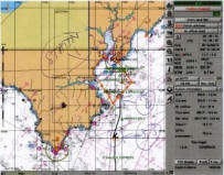
Fig. 1. Ships tack with stations 1, 2 & 3 labelled.
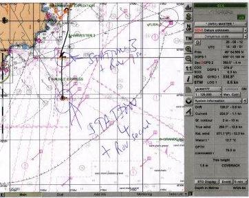
Fig. 2. Ships track to show station 4
Fig . 3. Vertical profile for station 1
Fig. 4. Vertical profile of station 2
Fig. 5. Vertical profile of station 3
Fig. 6. Vertical profile of station 4
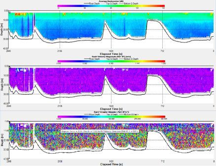
Fig. 7. ADCP data for station 1
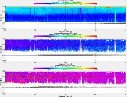
Fig. 8. ADCP data for station 2
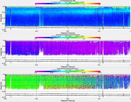
Fig. 9. ADCP data for station 3
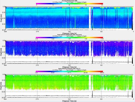
Fig. 10. ADCP data for station 4
Fig. 11. Richardson number against depth
Fig. 12. Percentage composition of phytoplankton at stations 3 & 4
Fig. 13. Percentage composition of zooplankton species at the 4 stations
Fig. 14 Relative composition of dominant phytoplankton species at stations 3 & 4
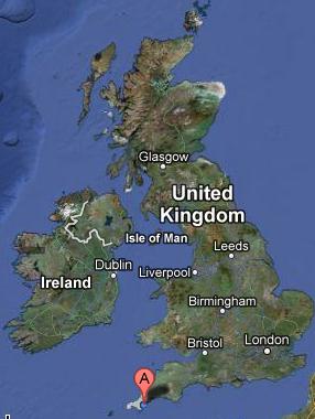
Fig. 15. Shows the location of the transects in relation to the UK
Introduction:
General site area and background:
The Fal estuary is located off the English South Coast; many areas along the Fal estuary are designated as Special Areas of Conservation (SAC) sites by Cornwall council 2012. It consists of a number of broad, shallow inlets and bays, salt marshes, intertidal mudflats and sub-tidal sandbanks.
|
Date: 26/6/12 |
Instruments used: Sidescan Sonar |
|
Vessel: S.V. Xplorer |
Drop cam |
|
Departure: 07.25 GMT |
|
|
High water: 12:38 GMT: 4.40m |
Crew: 14 |
|
Low water: 06.38 GMT: 1.30m |
|
Aims:
1. 1.Create a habitat map of a selected area in the Fal Estuary, using acoustic sidescan sonar along transects.
2. 2.Provide video data within the surveyed area to provide evidence of sidescan results.
3.Observe and record any changes in the habitat type along each survey transect.
Methods:
A sidescan sonar towfish was deployed into the estuary at a depth of approximately 1m. The vessel was then manoeuvred in order to tension the line connecting the fish to the vessel so the depth did not alter. The vessel was positioned at the beginning of each transect and a printout of the sidescan data was initiated. The vessel travelled at a constant velocity following the track that had previously been decided upon by the navigator and skipper. The end of each transect was marked on the printout this process was carried out until all the transects had been completed, the fish was then recovered to the vessel and the drop cam was prepared for deployment.
In consultation with the navigator and the group a transect was plotted for the dropcam to be deployed in areas of interest as reliable locations using the sidescan and dropcam. The drop cam allows for a greater degree of accuracy in determining the cause of any increases or decreases in backscatter from the sidescan, it also gives the benefit of being able to identify the key species that reside in the area.
|
Drop Site |
Location |
Time (AST) |
||
|
Longitude |
Latitude |
Deployed |
Recovered |
|
|
1 |
005o 01’58.896 W |
50o11’31.02 N |
10:44:00 |
10:47:15 |
|
2 |
005002’04.7256 W |
50o11’41.98 N |
10:50:35 |
10:54:48 |
|
3 |
005001’46.871 W |
50011’15.379 N |
11:11:30 |
11:20:54 |
Results:
|
First Drop Site |
Second Drop Site |
Third Drop Site |
|||
|
Marcoalgae |
Benthic species |
Marcoalgae |
Benthic species |
Marcoalgae |
Benthic species |
|
Rhodophyta |
Molluscs (scallops, invasive slipper limpets) |
Rhodophyta |
Few due to nearly 100% algal benthic coverage |
2 Rhodophyta species |
Similar to other sites: Sabella (site with highest abundance), scallops, sand mason worms, fish species (possible juvenile pelagic species) |
|
Chlorophyta |
Annelids (Sabella worms) |
Chlorophyta |
Low diversity, high dominance |
2 Chlorophyta species |
|
|
High density Chlorophyta, dominance |
Sand mason worms |
Greater density than site 1 with chlorophyta dominance over rhodopohyta |
Some sediment patches with mollusc shell covering |
Equal Chlorophyta and Rhodophyta distributions |
Exclusive to site 3: Decapods, hermit crab, Benthic crab, gastropod shell |
|
Fish species similar to Mottled Sculpin |
|||||
Discussion:
Habitat Mapping:
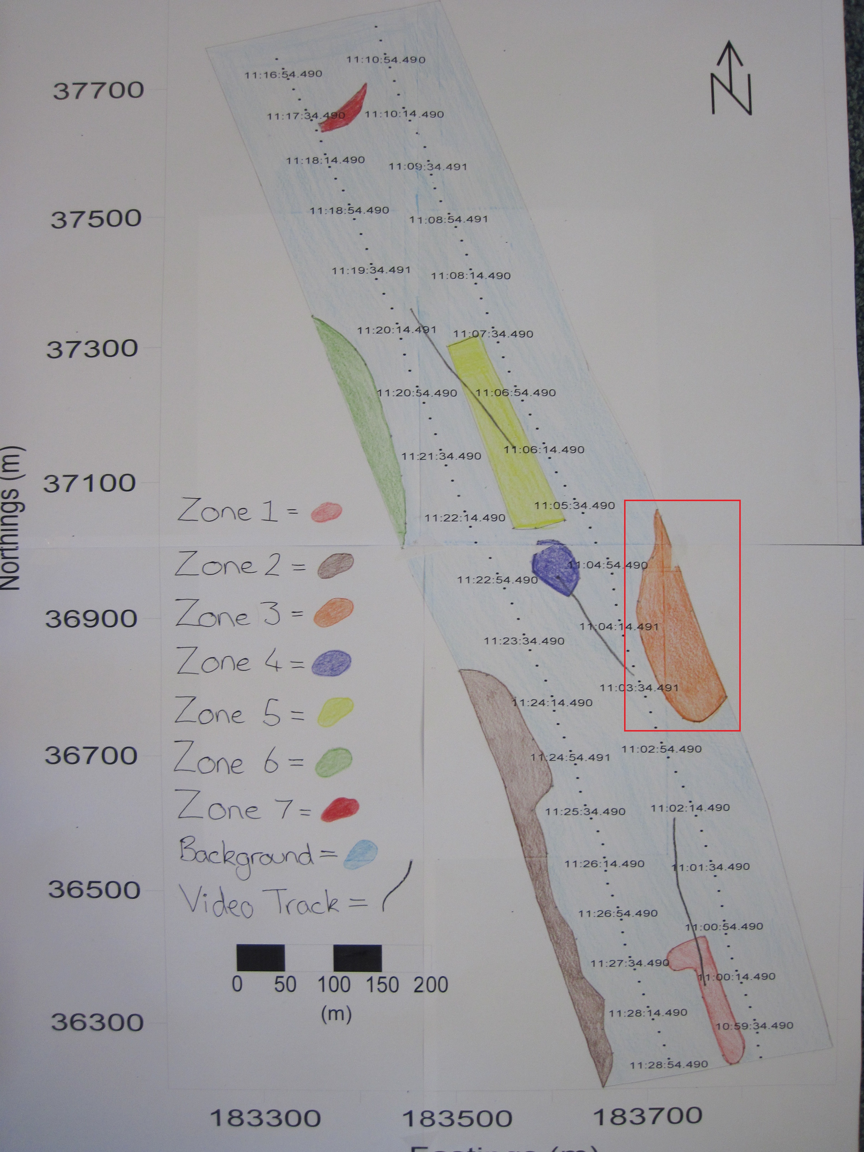
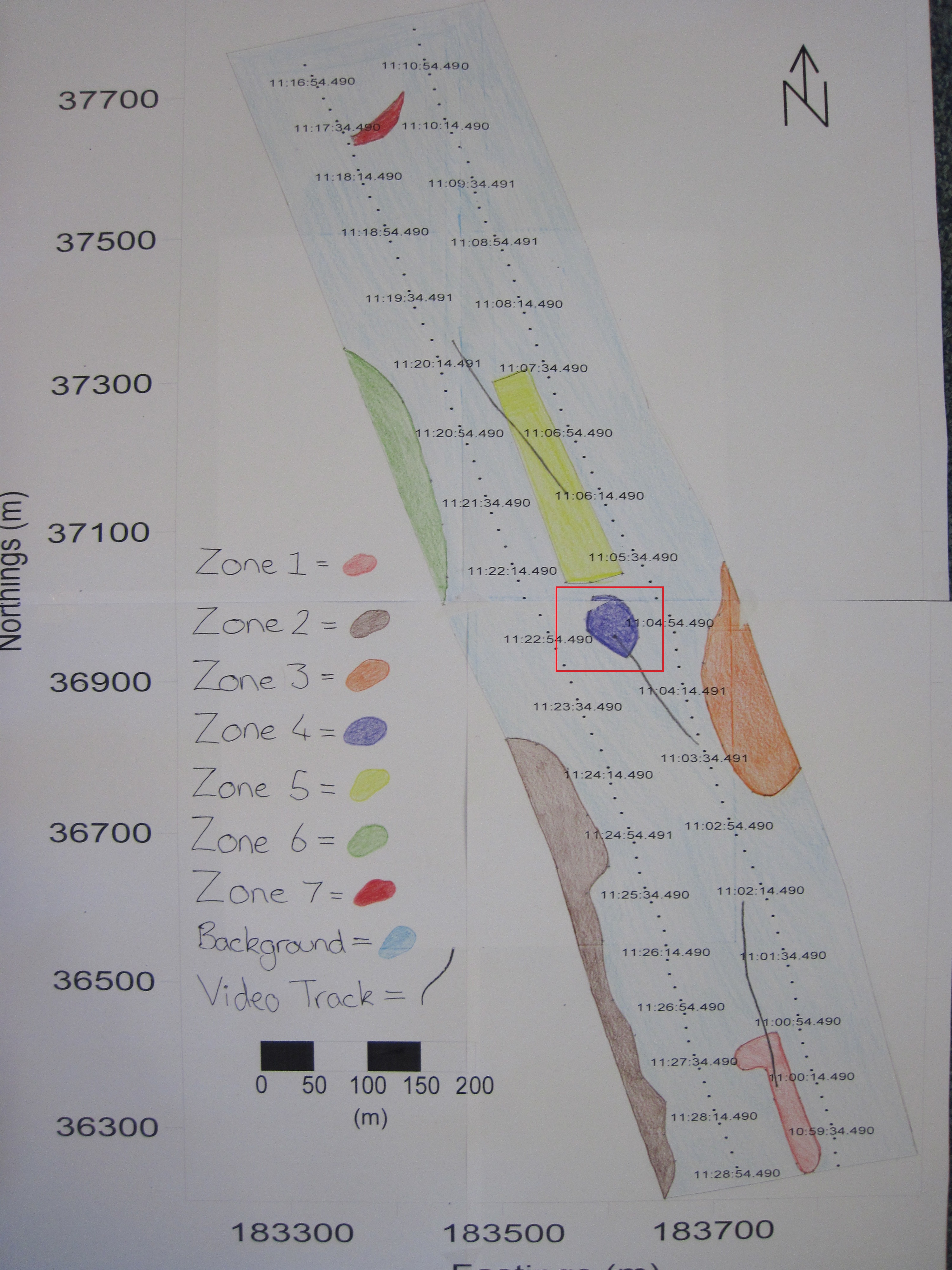
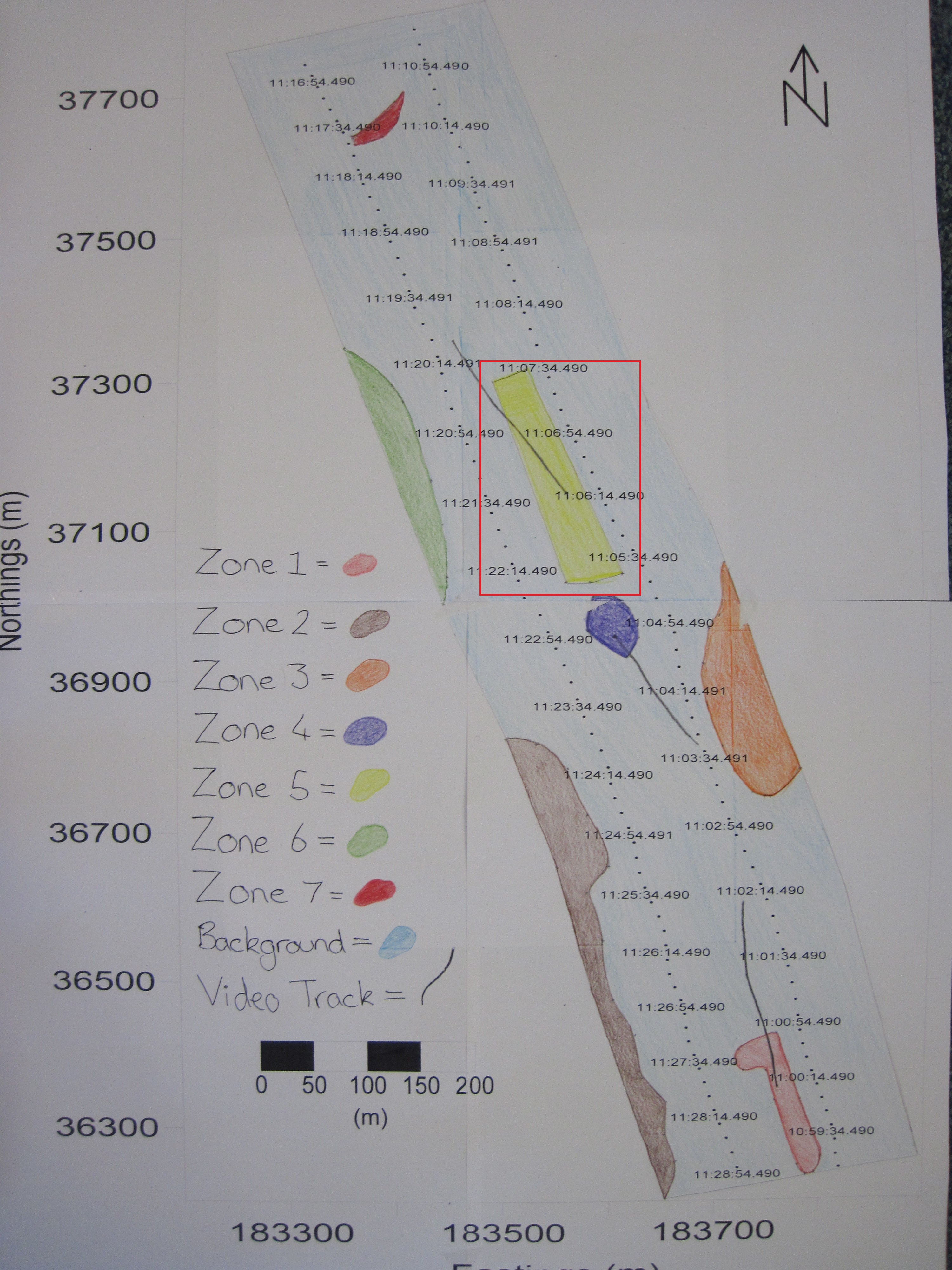
(Fig. 18)
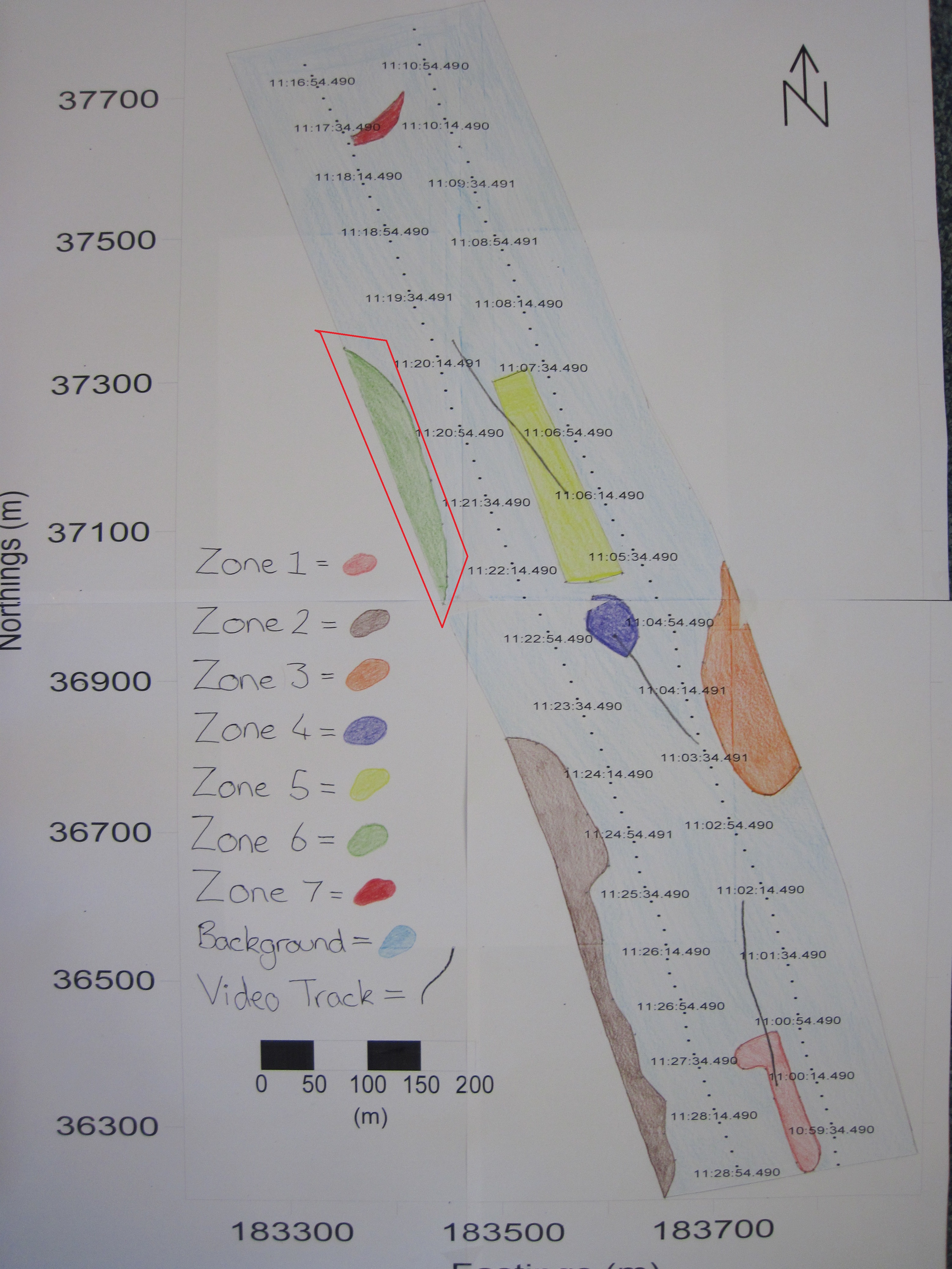
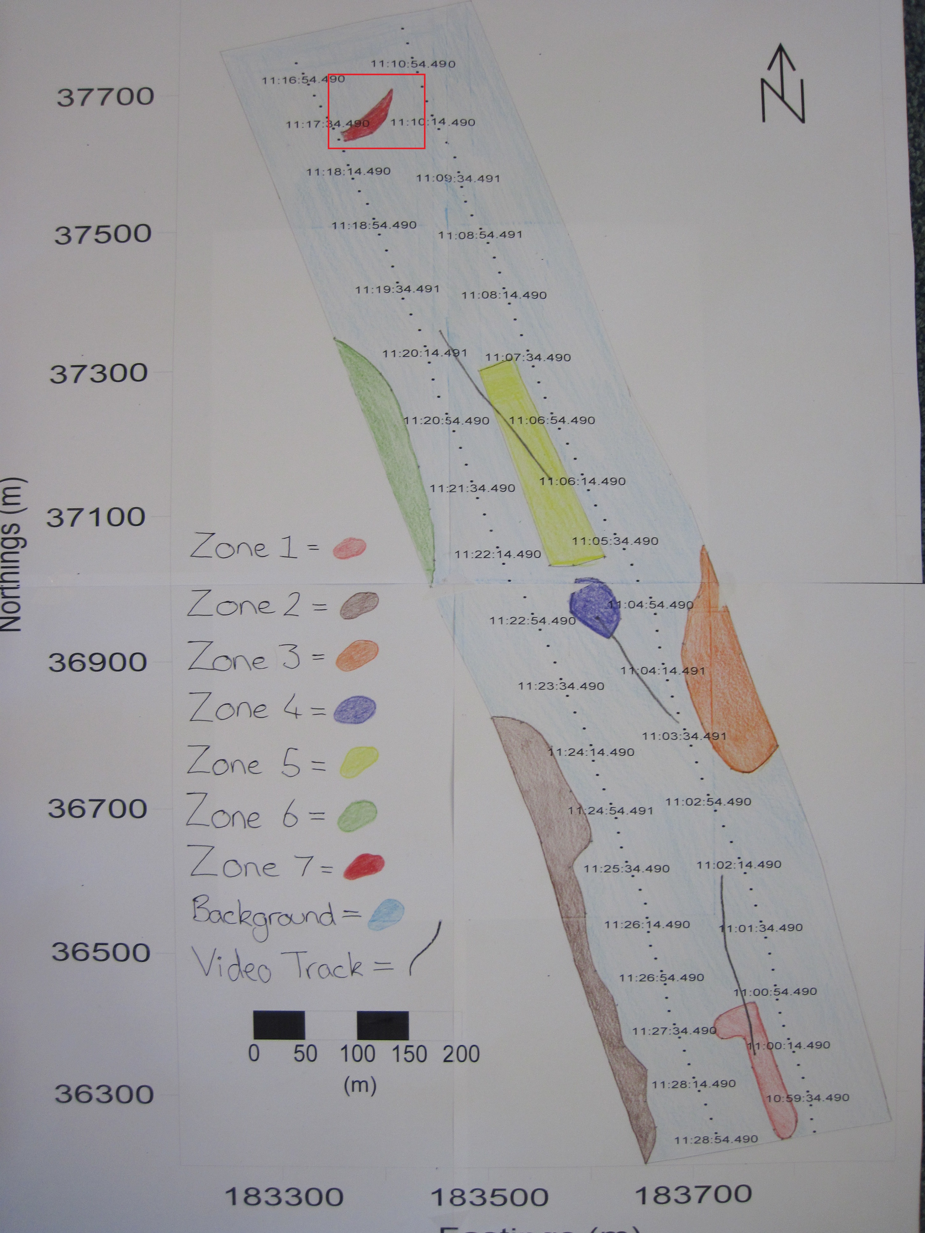
Sidescan data showed a change in composition in sediment along transects from south to north going from coarser to finer material. Zone 1 showed coarser sediment, dropcam video of the area indicated the prescence of shells. Dropcam video in Zone 2 displayed a higher proportion of shells compared to zone 1, this could be due to more favourable conditions for organisms with shells. Zone 3 showed a diagonal bedform pattern created by the river Fal. Zone 4 showed raised isolated seabed depicted by a shadow on the trace. Zone 5 showed coarser sediment consisting of shell or gravel, indicated by their presence in the dropcam video footage, in higher abundance to the South and fading out to the North, possibly due to currents. Zone 6 showed a similar pattern to zone 2, with coarser sediment and more shells present. Zone 7 showed finer sediment, with soft mud, shells and macroalgae present; seen in the dropcam video.
Dropcam:
Site 1:
The first dropcam site, deployed in the middle of the transect showed macroalgae such as Rhydophyta and Chlorophyta, with the Chlorophyta more dominant. It also showed the presence of benthic species such as; molluscs, scallops and the invasive slipper limpet species Crepidula fornicata, along with annelids such as Sebella worms and sand mason worms. There were also several species of fish seen such as Motted Scuplin.
Site 2:
The second dropcam site, taken at the northern end of the two transects showed Rhydophyta and Chlorophyta present at higher densities than in the first drop site with Chlorophyta dominance over Rhydophyta. There was a much lower abundance of benthic species seen at this drop site compared to the previous drop site due to almost 100% algal benthic coverage. There were some patches of sediment present that were covered with mollusc shells.
Site 3:
The third dropcam site, was carried out at the southern end of the sample zone between the two transects. This video footage showed two species of Rhydophyta macroalgae along with two species of Chlorophyta in equal abundance and distribution, therefore showing less dominance of one species over the other. The benthic species seen here were similar to the previous two sites, with Sabella in high abundance, scallops, sand mason worms and several fish species, including the possiblility of juvenile pelagic species. This drop site also had some benthic species that were exclusive, including decapods, hermit crabs, benthic crabs and gastropod shells.
Conclusion:
The habitat mapping, predicted using the sidescan sonar, can be supported and further analysed using the video footage from the dropcam. Overall data shows that the benthic habitat in that area of the estuary is relatively homogenous, with gradations in the density of macrofauna and macroalgae. Sediment was generally coarser to the South and finer towards the North. This is due to the strong tidal currents carrying finer sediment further North into the estuary, but depositing the coarse sediment in the South at the mouth of the estuary.
The use of the dropcam combined with the sidescan allowed further investigation into the habitat mapping of the sites studied. It gave an insight into species composition and the variation within the niches present. The use of the drop cam showed changes in the macrofauna and macroalgae abundance and displayed notable differences within the sites studied, but also showed similar species composition between the three sites. Site 3 had the highest biodiversity. This is a notable difference as this site was the only one studied that did not have any Crepidula fornicata, an invasive species. This could be because the absence of this species has allowed further development of niches, permitting a higher species diversity.
Other factors affecting the seabed and therefore the species diversity, include the relatively high-energy wave action (Hall–Spencer, 1991). This would affect some organisms if they are not adapted to high energy environments. The high-energy wave action may increase sedimentation of the surrounding areas, and therefore affecting the conditions that are available for colonisation. For example, some suspension feeders would find it hard to survive in such areas due to their gills becoming clogged, eg. sipunculid worms. The high level of ship activity seen in Falmouth Bay would also increase vertical mixing, and increase turbidity, decreasing available light (Newton, 2011) and therefore alter the habitat in which the organisms live. These influencing factors combined with the evidence from the sidescan and the dropcam video footage allow the state of the seafloor to be analysed and mapped.
Further investigation:
To investigate the habitat mapping further several sediment grabs were planned to be taken, but due to the development of marine conservation zones in relation to the density of maerl, these are no longer allowed unless a license is held allowing grabs to be taken. This posed a limitation on the study, however no maerl was seen in the two transects studied. This could be because near to the transects studied there were crab pots, and maerl is susceptible to mechanical damage such as done by these pots and anchoring near to the area (Newton; 2011).
![]()
![]()
Fig. 16. Expands of fig. 14. and gives the location relative to Prince of Wales pier located in Falmouth
![]()
Fig. 17. Gives the relative distance of the transects from the shore and each other. Also shows the initial transect before the course of action was altered.
Fig. 18. A habitat map produced based on sidescan data and video evidence around the two transects carried out
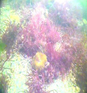
Fig. 19. An image taken from the drop cam video
Pontoon:
Introduction:
|
Date: 03/7/12 |
Instruments used: |
|
|
Location: Pontoon: 050o12’57.83 N, 005o01’39.42W |
YSI multi probe, Li-cor light meter, |
|
|
Departure: 08.30 GMT |
Analogue current meter |
|
|
High water: 05:25 GMT (4.9m) |
||
|
Low water: 12:10 GMT (0.60m) |
Heading: N/A |
Crew: 9 |
|
Station |
Time |
Weather |
|
Pontoon |
09:00 |
100% Cloud cover, 11.5mm rain, 20mph SW wind |
|
12:00 |
100% Cloud cover, 0.6mm rain, 20mph SW wind |
Data was collected at regular 15 minute intervals to observe how the temperature, salinity, current speed, pH, irradiance, chlorophyll concentrations and dissolved oxygen change of the period of a tidal cycle. All these measurements can be used to begin to understand the dynamics of estuarine systems as it is important because they act as mediums for the transport of waste, contaminants and pollution which affect the surrounding local biota. As estuaries are semi enclosed they tend to be the first point of impact of the pollutant or waste and control the form and concentrations of the pollutants once they reach the sea.
Results:
Surface (fig. 22)
Salinity decreases from 31.6 at 08:40 GMT to 28.91 at 11:40 GMT. The temperature increases from 14.80°C at 08:40 GMT to 15.70°C at 11:40GMT, the temperature increases relatively steadily between 08:40 GMT and 11:25 GMT before rapidly increasing to 15.70°C at 11:40 GMT. There is a minor peak in temperature at 10:10 GMT with a value of 15.10°C, this could be related to the minor trough in Salinity of 29.16 at 10:25 GMT. At the surface, pH varies over time but with a general increase between 8.68 and 8.70. The variations are small in context, so it could be interpreted that the pH remains steady throughout the tidal cycle. The % irradiance stays fairly constant between 08:40 GMT and 10:10 GMT with values ranging between 0.52% and 0.65%. There is a decrease down to 0.20% at 10:40GMT which then increases to 0.62% at 11:10 GMT and decreases again to 0.18% at 11:40 GMT. The current speed varies over time but generally there is a decrease between 0.23m/s at 08:40 GMT to 0.11m/s at 11:40 GMT with most values fluctuating between 0.00m/s and 0.27m/s with the exception of the abnormal current speed peak of 0.42m/s at 10:55 GMT. Chl a concentrations increase between 5.6µM at 08:40 GMT to 8.6µM at 11:40 GMT, with a minimum value of 5.4µM at 09:25 GMT and a mini peak with a value of 5.9µM at 09:40 GMT which coincides with the time of a dip in current speed and pH. Dissolved oxygen decreases between 96.50% at 08:40 GMT to 95.60% at 09:10GMT, then increases to a maximum value of 97.40% at 11:40 GMT. There is a small dip in DO% at 11:10 GMT where DO drops from 96.60% to 96.00% and back up to 97.00% at 11:25 GMT.
1m (fig. 23)
Salinity decreases steadily at 1.00m depth between 31.7 at 08:40 GMT to 28.95 at 11:40 GMT. Temperature increases steadily between 14.840C at 08:40 GMT to 15.170C at 11:40GMT, with the exception of a peak between 10:10 GMT and 10:40 GMT with maximum temp of 15.40C at 10:25 GMT. The pH at 1m depth follows the same pattern as at the surface. The % irradiance remains constant throughout most of the time recorded ranging between values of 0.18% and 0.28%, with the exception of 11:10 GMT where the value reaches 0.62%. The current speed follows the same pattern as the surface data, with minimum value of 0.04m/s at 11:10 GMT and a maximum value of 0.40m/s at 11:40 GMT. The Chl a concentration increases between 5.1µM at 08:40 GMT and 8.2µM at 11:40 GMT with a dip at 11:10 GMT, with a value of 6.2µM, that fits with the peak in % irradiance at this time. Dissolved oxygen follows the same pattern as surface, decreasing between 96.50% at 08:40 GMT to 95.60% at 09:40 GMT and then increases to 97.70% at 11:40 GMT.
2m (fig. 24)
Salinity follows the same pattern at 2m depth as at 1m and the surface. Decreasing from 31.90 at 08:40 GMT to 29.46 at 11:40 GMT. Temperature also increases steadily from 14.800C at 08:40 GMT to 15.110C at 11:40 GMT. The pH shows a similar pattern to shallower depths, however at 11:40GMT there is a maximum pH of 8.74, an absolute maximum for the entire dataset. % irradiance shows a general decrease over the time recorded with a maximum value of 0.19% at 09:55 GMT and a minimum value of 0.05% at 11:10 GMT. Current speed varies between a minimum of 0.08m/s at 10:40 GMT and 0.30m/s at 08:40 GMT, with an overall decrease between 08:40 GMT and 11:40 GMT. Chl a concentration increases over the time recorded, with a minimum value of 5.00µM at 08:40 GMT and a maximum value of 6.5µM at 11:25 GMT. There is a minor peak of 6.2µM at 10:10 GMT. Dissolved oxygen, again, follows the same pattern as shallower depths, with a decrease from 96.30% at 08:40 GMT to 95.50% at 09:40 GMT and then an increase to a maximum of 96.90% at 11:40 GMT.
3m (fig. 25)
Missing data is due to the fact that not every instrument could measure down to 3m at all times as the water depth was sometimes shallower than 3m as the tide went out. Salinity decreases from 32.12 at 08:40 GMT to 30.30 at 10:25 GMT, then starts to increase again but no data was taken past 10:40 GMT. Temperature increases steadily from 14.760C at 08:40 GMT to 14.970C at 10:25 GMT, then decreases rapidly in the next 15 minutes but then no further data was taken. The pH follows the same pattern as depths above 3m. % irradiance generally decreases throughout the time recorded with a maximum value of 0.06% at 09:10 GMT and a minimum value of 0.01% at 11:25 GMT. The current shows a general decrease over the recorded time, with a minimum value of 0.00m/s at 10:10 GMT and a maximum value of 0.29m/s at 08:40 GMT. Chl a concentration increases from 5.0µM at 09:10 GMT to 6.9µM at 11:40 GMT. Dissolved Oxygen decreases from 96.10% at 08:40 GMT to 95.00% at 11:25 GMT.
Irradiance profiles:
Figure 27 shows that the percentage irradiance decreases with depth for all the times measured throughout the morning. They all follow a similar pattern apart from times 10:25 and 11:10. The graph also shows a line to represent the 0.1% irradiance. This line denotes the 10% light level, below this depth no net photosynthesis occurs. The graph also shows a 0.01% light level line, or the critical depth line, which represents the depth at which photosynthesis can no longer occur. The graph shows that across all the times sampled, photosynthesis can take place down to the depths measured. All but two of the times sampled show a decrease in the light level that can penetrate down to the lowest depth measured. This is because the light is absorbed and scattered throughout the water column and this leads to lower readings. Line 10:25 does not follow the same pattern can be explained by a cloud covering the sun at the time of measurement, and therefore reducing the light available to penetrate the water. Line 11:10 can be explained by an increased light availability, and hence the light can penetrate further into the water and give a higher irradiance reading.
Figure 26 represents a time series of the 0.1% irradiance level, or the compensation depth. This shows how the depth of this level of light changes over time. The graph shows a decrease in the depth that light penetrates to. This means that this is the limit at which net photosynthesis can no longer occur. The 0.1% irradiance level was plotted as opposed to the 0.01% level as photosynthesis can occur to the depths measured, therefore a time series could not be made. The decrease in the 10% light level shown in the figure can be correlated to the tide times of the area. During the sampling times, the tide was going out; low tide was at 12.10 UTC. This explains why the depth of the 10% light level decreased as there would be more sediment and particles in the water due to the increased level of mixing. The graphs show that the penetration of photosynthetically active radiation (PAR) into seawater depends on the nature of the light penetrating the water and the absorbing properties of the water and the substances within it (Anderson; 1991). In turn, the attenuation and photosynthesis are affected by the spectral properties of the light field.
Estuary:
Introduction:
|
Date: 04/7/12 |
Instruments used: |
|
|
Vessel: RV Bill Conway |
ADCP, CTD, Niskin bottle, Secchi Disk, Fluorometer, |
|
|
Departure: 08.20 GMT |
Transmissometer, Plankton net |
|
|
High water: 05:19 GMT, 5.00m |
||
|
Low water: 12:04 GMT, 0.40m |
Heading: Towards the Mouth |
Crew: 13 |
|
Station |
Latitude |
Longitude |
Arrival (UTC) |
Departure (UTC) |
Weather |
|
1 |
50°12.186N |
005°02.459W |
12:01 |
12:46 |
20% Cloud cover, 11mph SW wind |
|
2 |
50°11.662N |
005°02.681W |
12:54 |
13:22 |
50% Cloud cover, 11 mph SW wind |
|
3 |
50°10.0043N |
005°02.1835W |
13:39 |
14:15 |
40% Cloud cover, 13 mph SW wind |
Aims:
1. What is the physical structure of the Fal estuary (i.e. mixed, partially-mixed, stratified? What is the flushing time of the estuary ?
2. How does the physical structure change from the rivers through the estuarine and sound zone and off shore to the Channel station ?
3. How do the tides affect the conditions within the estuary and the adjacent coastal region through time?
4. What is the nutrient environment within the estuary, and how conservative are the nutrients?
5. What levels of algal biomass are there in the estuary (and how do they compare to offshore)? Is the biomass related in any way to the nutrient distributions?
6. How turbid is the estuary? What is causing the turbidity? How quickly is light attenuated through the water column in the estuary? How does this compare to the offshore region?
7. What is controlling / limiting primary production within the estuary (and is that different to offshore)?
8. Are the estuarine planktonic communities different to those further offshore?
Method:
Sampling
The ADCP was recording data continuously along a transect of the estuary to measure the flow rate and direction of the water masses below the vessel as well as the volume of water moved per second, this will allow for an estimate of residence time of the estuary to be calculated.. At each station, a CTD was deployed with a transmissometer and a fluorometer attached to the system. These instruments were used to provide information about the characteristics and stratification of the water mass at different stations and allow for comparisons between each. A Niskin bottle was deployed at each station and used to collect samples for specific depths. The bottle was lowered to the required depth then a brass messenger was allowed to slide down the hydroline causing a sample of water to be trapper within at this depth. the sample was then collected for later analysis of the nutrient, dissolved oxygen and chlorophyll compositions within it. Phytoplankton and zooplankton were collected in a net, which was deployed from the stern of the Conway. Weights were attached to the bottom of the net to pull it down to the required depth. After a trawl of 5 minutes the net was recovered to deck and washed with a hose to ensure all of the phytoplankton and zooplankton were collected within the bottle at the “cod end” of the net. A secchi disk was deployed at each station to attain a measure of the turbidity of the water thus allowing for the depth of the euphotic zone to be calculated. When a chlorophyll maxima was noticed on the CTD plot a sample was taken at that depth and later analysed to identify which species of phytoplankton were present.
Analytical
Silicon, Phosphate and Chlorophyll:
Carried out as per Parsons et al. 1984
Nitrate:
Flow injection method as per Johnson, K et al. 1983
Dissolved Oxygen:
Carried out as per Grasshoff, K et al. 1999
Results:
Vertical Profile:
Station 1:
Figure 30 shows a decrease in temperature with depth, starting at a temperature of 15.000C at the surface, to 14.380C at 2.83 meters. The temperature then increases again to 14.520C at 4.71 meters. The temperature then decreases steadily to 13.110C at 13.62 meters. Salinity increases with depth, starting at 30.52 at 0.4 meters depth, before decreasing steadily to 34.599 at 13.62 meters. Fluorescence increases from 0.21mg/m3 at 0.21 meters, to 0.24 mg/m3 at 2.83 meters. There is a notable peak at 0.36mg/m3 at 5.13 meters. Fluorescence remains fairly stable before increasing again at 0.314 mg/m3 at 13.22 meters. Chlorophyll has a prominent peak at 5 meters with a concentration of 4.57 ugL-1; the chlorophyll max. Silicon decreases with depth, with a concentration of 13.05 µM at 1.00 meter, to a concentration of 6.51 µM at a depth of 9.00 meters. Nitrate is also shown to decrease with depth, with a concentration of 3.71 µM at 1.00 meter, to a concentration of 1.29uM at a depth of 3.00 meters. Dissolved oxygen levels increase with depth, with a saturation of 62.6% at 1.00 meter, to a percentage of 75.5 at 9.00 meters. Phosphate decreases with depth from 0.0092 µM at 1.00 meter to 0.0082 µM at 5.00 meters, and then increases again to 0.0084 µM at 9.00 meters.
Station 2:
At station 2, temperature and salinity decrease gradually throughout the water column (Fig. 31). Though, temperature drops from 14.14°C at 2.05m to 13.64°C at 6.06m. Salinity increases going down the water column and it jumps from 30.25 at 3.16m to 31.18 at 6.27m. Therefore it is possible to say that temperature shows a slight thermocline and salinity shows a small halocline around the same depth indicating that the water column is stratified. This agrees with the ADCP data which show only partially different water masses. This is expected as station 2 which is closer to the mouth of the estuary where the saltwater input from the sea is stronger and the freshwater coming down the Fal estuary sits on atop. In fact freshwater is less saline as it contains less heavy ions; furthermore it is warmer than seawater and therefore more buoyant. Fluorescence peaks at 2.80m with 3.32mg/m3, which is very close to the maximum chlorophyll value of 8.51µg/L at 1.5m indicating that a chlorophyll maxima and that most of the phytoplankton is found around this very shallow depth. This agrees with the backscatter data from the ADCP which is highest at this depth. As the depth of the euphotic zone worked out with the Secchi disc was around 6.99m, it was expected to find phytoplankton more distributed down the water column. Though silicon, nitrate and phosphate are in their highest concentration at 1.5m depth, therefore phytoplankton is probably concentrated at this depth in order to benefit of the relatively high concentrations of nutrients. In fact despite being the highest concentrations for station 2, the nutrient level are rather low, but this is expected at this time of the year as starting from end of April, increased solar radiations provide enough stratification to allow the phytoplankton to bloom, but therefore utilise nutrients in large amounts. The percentage of dissolved oxygen is highest at 5m with 71.90%, however all the values are under 100% indicating that water is under saturated therefore suggesting the presence of a large amount of phytoplankton which consume oxygen by respiration.
Station 3 (fig. 32):
Temperature decreases quite rapidly from 13.940C at the surface to 13.330C at 4.2m, then remains stable at that temperature between 4.2m and 14.86m, before decreasing again to 12.830C at 20.3m. Salinity follows an inverse pattern to temperature, increasing from 34.2 at the surface to 34.6 at 4.5m. The salinity remains fairly stable, increasing slightly between 4.5m and 15m to a value of 34.9. The salinity below this depth gradually increases to a maximum of 34.9 at 20.3m. The Fluorescence fluctuates between a maximum of 0.3790mg/m3 at 11.3m and a minimum of 0.1640mg/m3 at 17.4m. The fluorescence loosely follows the salinity and temperature stratification where values are generally higher above 5m, slightly lower between 5m and 15m and then lower still below 15m. The nutrient data was taken at a limited number of depths down to 9m, so the lines connecting data points on this graph are interpolated. Chlorophyll appears to increase from the surface down to a peak at 1.5m with concentration 11.2320ug/l. Chl concentration then decreases below this depth. Silicon decreases with depth from a maximum of 4.1079uM at 1m to a minimum of 3.5685uM at 5m. This value then increases slightly with depth. Dissolved oxygen follows the chlorophyll pattern, first increasing with depth to a maximum of 77.1% at 3m, then decreasing to a minimum of 62% at 5m depth. Phosphate increases with depth to a maximum of 0.007673uM at 5m then decreases below this depth.
Estuarine Mixing:
Nitrate (fig. 33):
Data was only collected from the lower part of the estuary, and the riverine end member was given to us to enable the mixing diagram to be plotted. The mixing diagram results of the Nitrate concentration versus salinity analysis conducted indicated conservative behaviour. For conservative behaviour in an estuary concentration is determined by mixing of marine and riverine end-members. This is due to the data points being concentrated at between 28.1-34.6 salinity and 0.71-5.71 µm nitrate concentrations plotting along the Theoretical Dilution Line. There were three riverine end members which were averaged to 0.10 salinity and 28.57 µm nitrate concentration. The Sea Water End Member was 0.93µm and a salinity of 34.60, with the Riverine End Member averaged at 28.57µm and 0.10 salinity.
Phosphate (fig. 34):
Data was only collected from the lower part of the estuary, and the riverine end member was given to us to enable the mixing diagram to be plotted. The data collected from the lower part of the estuary shows phosphate behaving non-conservatively initially. However, there is not enough data to presume that phosphate is non-conservative throughout the estuary. This data shows addition of phosphate between salinities of 28.10 and 35.10. The riverine end member had a concentration of 0.0154µM at salinity 0, and the marine end member had a concentration of 0.006926µM at salinity 35.10.
Silicon (fig 35):
Data was collected from the lower part of the estuary, and the riverine end member was given to us to enable the mixing diagram to be plotted. The data collected from the lower part of the estuary shows silicon behaving conservatively initially. However, there is only one data point between salinity 28.10 and salinity 0.30, therefore it would be unreliable to extrapolate to assume that silicon behaves conservatively throughout the estuary. The riverine end member had a concentration of 93.68µM at salinity 0.3 and the marine end member had a concentration of 3.0966µM at salinity 35.10.
Biological:
|
Zooplankton |
Station |
1 |
|
|
Station |
3 |
|
|
Taxa |
10ml |
10ml |
Total |
Corrected |
5ml |
5ml |
Total |
|
Copepoda |
30 |
23 |
53 |
26.5 |
23 |
30 |
53 |
|
Copepoda Nauplii |
46 |
7 |
53 |
26.5 |
91 |
103 |
194 |
|
Cladocera |
0 |
1 |
1 |
0.5 |
1 |
4 |
5 |
|
Decapoda Larvae (Crab/Shrimp) |
1 |
0 |
1 |
0.5 |
1 |
0 |
1 |
|
Cirripedia Larvae (Barnacles) |
6 |
2 |
8 |
4 |
0 |
10 |
10 |
|
Polychaeta Larvae (Worm) |
1 |
3 |
4 |
2 |
0 |
9 |
9 |
|
Gastropod Larvae (Snail) |
0 |
0 |
0 |
0 |
0 |
7 |
7 |
|
Chaetognatha (Arrow worm) |
0 |
1 |
1 |
0.5 |
0 |
0 |
0 |
|
Hydromedusae (Jelly Fish) |
16 |
19 |
35 |
17.5 |
6 |
32 |
38 |
|
Appendicularia |
5 |
0 |
5 |
2.5 |
0 |
6 |
6 |
|
TOTAL |
105 |
56 |
161 |
80.5 |
122 |
201 |
323 |
The zooplankton results show that the samples were dominated by copepods and their nauplii (fig.36), which contributed 66% and 76% at stations 1 and 3 respectively. There was also a large proportion of hydromedusae at both stations (22% and 12%), representing the second most abundant group (table above). There were almost twice as many copepod nauplii at station 3 by proportion, but in terms of sheer numbers, station 1 had only 14% as many (2650/l compared to 19500/l). The % composition of the 2 sites was not drastically different; 9 different groups were found at each site, and only 1 group was found at station 1 which was absent from station 2, and vice versa (table). However, the overall density of cells was found to be significantly different; station 1 contained <25% of number of cells per litre that station 3 (figure).
|
Phytoplankton |
||||||
|
Station 1 |
|
Station 2 |
3m |
Station 2 |
1.5m |
|
|
Species |
Tally |
Cells/ml |
Tally |
Cells/ml |
Tally |
Cells/ml |
|
Alexandrium spp. |
16 |
160 |
5 |
50 |
14 |
140 |
|
Chaetoceros spp. |
1 |
10 |
0 |
0 |
||
|
Coscinodiscus spp. |
24 |
240 |
10 |
100 |
7 |
70 |
|
Guinardia flaccida |
0 |
11 |
110 |
2 |
20 |
|
|
Guinordia delicatula |
0 |
1 |
10 |
0 |
||
|
Karenia mikimotoi |
2 |
20 |
0 |
0 |
||
|
Rhizosolenia imbricata |
0 |
3 |
30 |
0 |
||
|
Prorocentrum micans |
0 |
1 |
10 |
0 |
||
|
Rhizosolenia setigera |
0 |
1 |
10 |
0 |
||
|
Thallasiosira |
0 |
3 |
30 |
0 |
||
|
Pseudo-nitzschia |
0 |
3 |
30 |
0 |
||
|
Total |
430 |
380 |
230 |
The phytoplankton results show variation between the stations (fig. 38). Station 1 shows the highest density, whereby it was found to have 430 cells/ml (Table above). Dominance was different between each site; there was no single group which was universally dominant throughout the whole transect. Coscinodiscus dominated station 1, Guinardia flaccida dominated station 2 at 3m depth and Alexandrium at 1.5m (Table above; Fig. 38). Notably, the number of groups present varied greatly between samples; the surface of station 2 had the lowest number and therefore the lowest species diversity, with only 3 groups present, whereas the highest was station 2 at 3m depth, where there were 9 groups present (Figure 39). Station 1 had 4 groups present, 2 of which were diatoms and 2 dinoflagellates, although there was a higher diatom composition overall. The data suggests there is a higher diversity with more equitability at 3m than at 1m or 1.5m depth.
Physical:
ADCP:
Station 1 (fig 40):
The ADCP data shows the majority of the water columns backscatter to be relatively constant with a backscatter of around 70 dB. The velocity of the water column appears to be rather variable with the velocity greatly changing throughout the water column and across the transect . With the water moving anywhere between 0.01 to 0.30m/s The ships tract shows the average movement of the water column to be north going up the estuary. While the velocity direction graph shows the water column to be fairly similar with patches of water moving in different directions.
Station 2 (fig 41):
The ADCP data shows that there is not much change in backscatter throughout the water column with the lowest backscatter being at the bottom of the water column at a depth of 14 m with a backscatter of 70dB. There is a higher peak of backscatter at the start of the transect 1 meter deep with a backscatter of 91. The velocity graph shows that the bottom waters are moving faster than the top waters. The waters from 5m to 14m are moving between 0.20m/s to 0.30m/s while the waters above about 5m moving between 0.05m/s to 0.20m/s. The ships track shows the average movement of the water column to be north up the estuary. The velocity direction graph shows the water column from 3 m to 14 m to be moving northwards while the first 2 m of the water column show the water moving slightly more north west.
Station 3 (fig 42):
Due to the depth range of the ADCP being limited to 20m the ADCP was not able to give a continuous recording across the channel. Therefore the ADCP data becomes more difficult to use. Backscatter on the edges of the channel is between 62-70dB. At the edges of the channel the velocity appears to be between 0.03m/s to 0.35m/s. At roughly 516m across the channel just before the ADCP data becomes blank there is a steep change in velocity up to 2.10m/s. However it is not possible to establish the velocity in the centre of the channel. The ships track either side of the channel shows the average flow to be towards the north this is backed up by the direction graph which shows the direction on either side of the central channel to be between 320-200.
Richardson Number (fig 43):
To calculate the Richardson number for the Estuary the density was calculated using an online converter from the depth, temperature and salinity. The CTD did not provide density therefore it had to be calculated. The website http://www.csgnetwork.com/water_density_calculator.html was used. This website referenced the calculation from, Millero, F Et al. (1980) The calculated density could then be used to provide a Richardson number using the data from the ADCP. For station 3 the ADCP was not consistent enough for the Richardson number to be calculated confidently for the channel.
Station 1
Station 1 shows Ri’s of above 1 consistently throughout the water column. This would suggest that there is a high likelihood of no mixing throughout the water column. With the least chance of mixing at 8 to 12 meters with an Ri of 38.22.
Station 2
Station 2 would suggest that there is no mixing at 0 to 2.5 meters and 5 to 8 meters with an Ri of 9.57 and 5.51 respectively. At 2.5 to 5 meters with an Ri of 0.29 it would suggest that there may be a likehood of mixing with an Ri of 0.29.
Residence time:
Tres (s) = (1-Smean/Ssea) x Vtotal (m³) = (1-33.92/36.51) x 25100903 =603458.66s =6.98days
R (m³/s) 2.06
Smean: 33.92 R: 2.95 m³/s
Ssea: 36.51 Vtotal: 25100903 m³
Total residence time is approximately 7 days.
The riverine flow rate was calculated from the combined flow rates of the Fal, the Kenwyn and the Kennal (Marsh & Hannaford 2008)
Volume calculated using ADCP data and Google Earth.
Assumptions Made:
-Width & depth of estuary remained constant between stations and were representative of water body.
-ADCP data covered full width of estuary.
-ADCP data where depth was >20m, ie at station 3 for group too, where ADCP could not read did not significantly alter the area.
-Sea water salinity taken at mouth of estuary is representative of sea water salinity.
-Average riverine flux rates are applicable.
-Fal, Kenwyn & Kennal are only input into system.
Discussion:
Profiles:
Station 1:
Station 1 shows that temperature decrease gradually with depth while salinity increases, though there are not sudden drops indicating a clear thermocline or halocline (Fig. 30). It is then possible to say that station 1 is only partially stratified which agrees with the ADCP data which show only slightly different water masses. In fact station 1 was located more landwards than station 2, therefore the freshwater input is larger while there is less seawater resulting into a more uniform water column. Fluorescence is inconstant throughout the water column but the overall trend is an increase from the surface where it has a value of 0.21mg/m3 at 0.21m to the highest peak which is of 0.36mg/m3 at 5.13 meters then a decrease, then it decreases again and peaks at 0.314 mg/m3 at 13.22m. Chlorophyll peaks at the same depth where fluorescence peaks that is 5m indicating a chlorophyll maxima. This suggests that most of the phytoplankton are concentrated around this depth which agrees with the depth of the euphotic zone worked out from the Secchi disc. The percentage of dissolved oxygen increases with depth, however the whole water column is under saturated with oxygen again indicating the presence of large amount of phytoplankton. Nitrate, silicate and phosphate decrease going down the water column, however there not enough nitrate value to provide a precise analysis. Silicate and phosphate are at lowest concentrations for this station around chlorophyll maxima which is found 5m and then they increase again indicating that phytoplankton is utilising nutrients.
Station 2:
At station 2, temperature and salinity decrease gradually throughout the water column (Fig. 31). Though, temperature drops from 14.14°C at 2.05m to 13.64°C at 6.06m. Salinity increases going down the water column and it jumps from 30.25 at 3.16m to 31.18 at 6.27m. Therefore it is possible to say that temperature and salinity show a small thermocline around the same depth indicating that the water column is stratified. This agrees with the ADCP data which show only partially different water masses. This is expected as station 2 which is closer to the mouth of the estuary where the saltwater input from the sea is stronger and the freshwater coming down the Fal estuary sits on top it. In fact freshwater is less saline as it contains less heavy ions; furthermore it is warmer than seawater and therefore more buoyant. Fluorescence peaks at 2.8m with 3.32 mg/m3, which is very close to the maximum chlorophyll value that is of 8.51µg/L at 1.5m indicating that a chlorophyll maxima and that most of the phytoplankton is found around this very shallow depth. This agrees with the backscatter data from the ADCP which is highest at this depth. As the depth of the euphotic zone worked out with the Secchi disc was of 6.99m, it was expected to find phytoplankton more distributed down the water column. Though silicon, nitrate and phosphate are in their highest concentration at 1.5m depth, therefore phytoplankton is probably concentrated at this depth in order to benefit of the relatively high concentrations of nutrients. In fact despite being the highest concentrations for station 2, the nutrient levels are rather low, but this is expected at this time of the year as starting from end of April, increased solar radiation provide enough stratification to the phytoplankton in order to bloom, and therefore utilise nutrients in large amounts. The percentage of dissolved oxygen is highest at 5m with 71.9%, however all the values are under 100% indicating that water is under saturated therefore suggesting the presence of a large amount of phytoplankton which consume oxygen by respiration.
Station 3:
At station 3 temperature is decreasing overall while salinity increases with depth (Fig. 32). Both parameters have steep gradients at around 4.5m depth where a thermocline and halocline can be identified, it is therefore possible to say that station 3 is stratified. This agrees with the ADCP data which show rather different water masses. This can be the result of the position of the station which is the by the mouth of the estuary therefore there is a large input of seawater and river water. When these two very different water masses get into contact the less dense, less saline freshwater which is more buoyant stays on top of the colder, denser and more saline seawater. Fluorescence is very inconstant, but it shows its maximum peak at 11.30m depth which is very close to the depth of the euphotic zone calculated from the Secchi dick, 11.40m. Fluorescence values roughly follow temperature and salinity stratification with values overall higher above 5m depth which could be due to the fact that phytoplankton cells are trapped in the upper part of the water column by stratification. This data agree with the chlorophyll values which peaks at 1.5m with a concentration of 11.23µg/l indicating the chlorophyll maxima of station 3. Although it is good to say that chlorophyll data were collected to a maximum depth of 9m while the CTD data by which fluorescence was measured cover 20m of the water column, therefore important chlorophyll variations could have been missed preventing a precise analysis. Dissolved oxygen values are all well under the saturation point of 100%, with the maximum value of 77.10% found at 3m, this suggests that phytoplankton are present in large number at station 3. This agrees with the nutrient data which are overall very low. The nutrients appear to decrease in concentration as going down the estuary despite the higher phytoplankton concentration found upriver. This could be due to the mixing between river water and seawater, in fact most of the nutrients, particularly silicon which is eroded by weathering from rocks, are brought to the sea by river input where they can be either simply diluted with sea water, added by physical and chemical processes or uptaken by phytoplankton (Kimmerer, 2005).
Biological:
Phytoplankton:
All nutrients decrease with distance downstream, so it would be logical to expect phytoplankton abundance, and therefore chlorophyll to increase, as this is used as a proxy for phytoplankton. However, this is not the case; Figure x shows that chlorophyll concentration in fact increases with distance downstream. This could be explained by the tidal state and the strength of flow in the estuary, which is compounded by mixing processes between fresh and saline water. Phytoplankton, such as diatoms, which are not motile and negatively buoyant so obliged to utilise turbulence in order to be re-suspended in the euphotic zone, have no control over their position on the water column and therefore may not be at the ideal location for primary production (Ross, 2006). The data shows that chlorophyll concentration increases downstream, despite phytoplankton decreasing in density. This could potentially be explained by the turbidity in the upstream part of the estuary, which reduced the capacity of the cells to perform photosynthesis. This is supported by the fact that there is around 25% of the number of cells per litre in the upstream areas. The cells here may also be mixed to a greater depth, further inhibiting photosynthesis.
Zooplankton:
Zooplankton are motile and therefore able to influence their position within the water column by vertical migration, controlled by endogenous circadian rhythms. However, this does not hold true for nauplii, which may explain the higher proportion of copepod nauplii in the lower parts of the estuary (station 1 has <14% of the concentration of station 3). This was also found in gastropod and polychaete larvae. The apparent inconsistency of the data may be due to the high stress environment and dynamic nature of the estuary, in which species composition and predator – prey interactions are highly variable temporally and spatially.
Conclusion:
From station 1 to station 3, therefore with increasing proximity to the estuary mouth, it is possible to observe stratification developing due to the mixing of the very different sea and river water. It is also possible to say that the Fal estuary has salt-wedge characteristics which are noticeable at all three station. In an estuary the salt wedge occurs when the river discharge is able to maintain a sharp gradient between freshwater and saltwater which have very different chemical compositions and therefore tend to mix very rapidly. Furthermore the salt wedge to occur the river flow has to be sufficient to counteract the mixing induced by tides or turbulence induced by wind (Ibanez et al. 1997). The salt wedge structure appears to influence also the position of the phytoplankton in the water column, which could be trapped by the stratified water. Furthermore also nutrients appear to be influenced by the salt wedge as most of them are carried by river water.
The residence time of the Falmouth estuary was calculated to be 7 days. However, it is difficult to comment upon the relevance of this value due to the high number of assumptions, averages and estimates that were used in order to calculate this value. Thus it should be taken as a rough guideline only, and not considered highly precise nor accurate. However it can probably be used as an order of magnitude estimate.
![]()
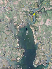
Fig. 20. Location of the pontoon in relation to Falmouth
Fig. 21. Overhead view of the pontoon
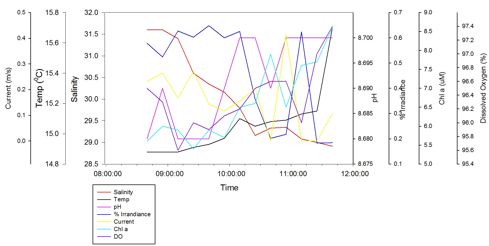
Fig. 22. Profile of data collected on the pontoon at the surface
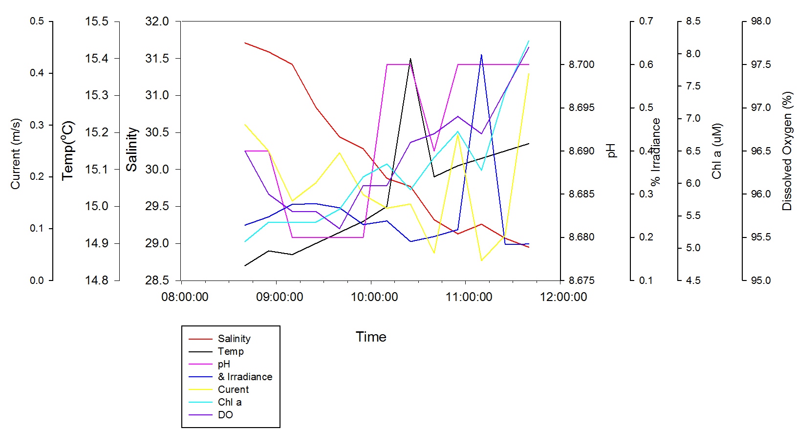
Fig. 23. Profile of data collected on the pontoon at 1m
Fig. 24. Profile of data collected on the pontoon at 2m
Fig. 25. Profile of data collected on the pontoon at 3m
Fig. 26. Representation of the 10% light depth over the course of a tidal cycle
Fig. 27. Depth off the 0.1% light depth at each individual time during the collection of the data set
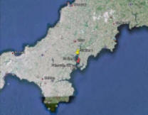
Fig. 28. Location of the Fal estuary
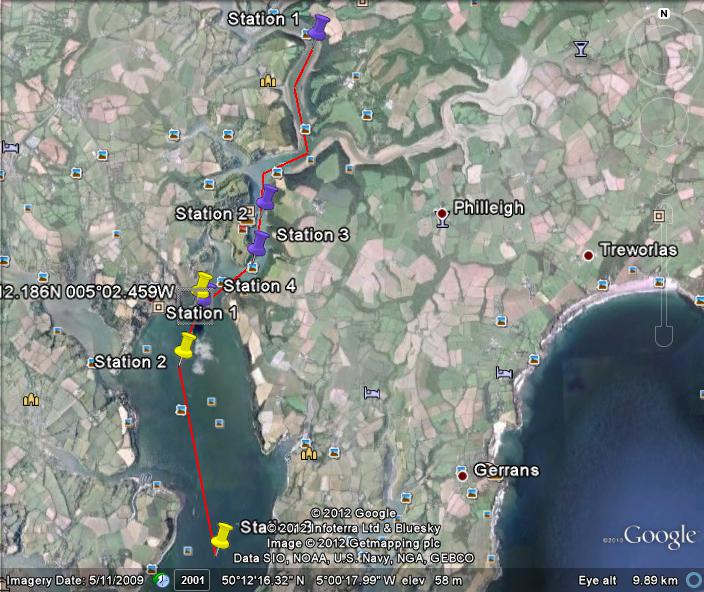
Fig. 29. Track and the locations of stations along the estuary carried out by groups 2 & 6
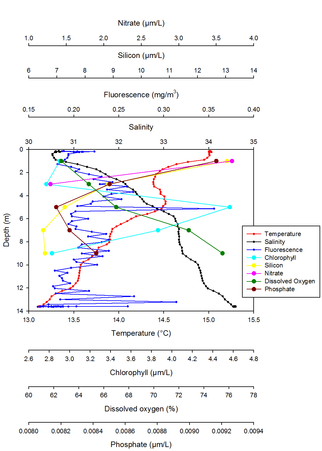
Fig. 30. Vertical profile for station 1
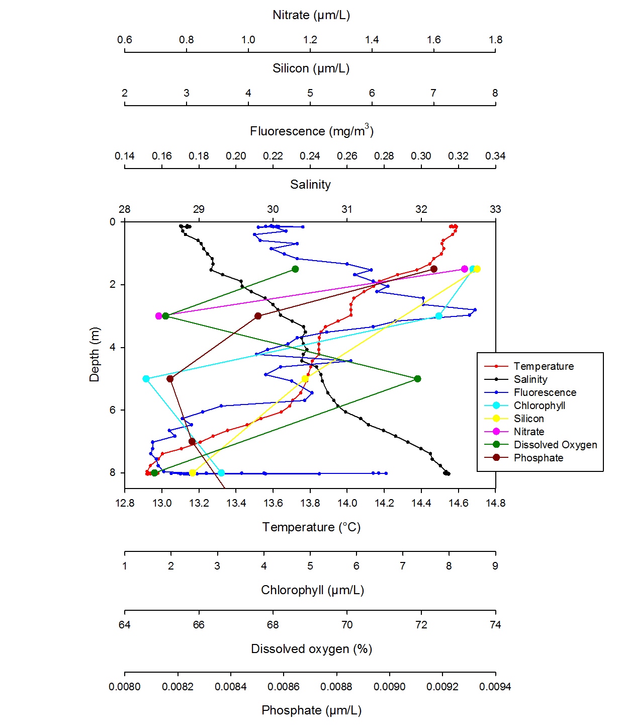
Fig. 31. Vertical profile of station 2
Fig. 32. Vertical profile of station 3
Fig. 33. A mixing diagram of nitrate within the estuary
Fig. 34. A mixing diagram representing phosphate within the estuary
Fig. 35. A mixing diagram representing silicon within the estuary
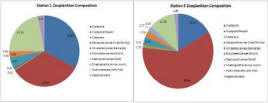
Fig. 36. Percentage composition of Zooplankton at stations 1 & 3
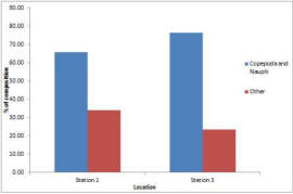
Fig. 37. Relative composition of dominant zooplankton species
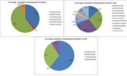
Fig. 38. Percentage Composition of phytoplankton at stations 1 & 2 (3m & 1.5m)
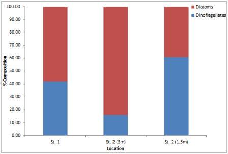
Fig. 39. Relative composition of the dominant at stations 1 & 2 (3m & 1.5m)
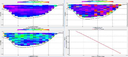
Fig. 40. ADCP data for station 1
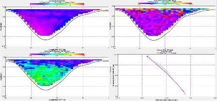
Fig. 41. ADCP data for station 2
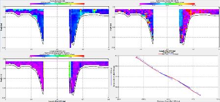
Fig. 42. ADCP data for station 3
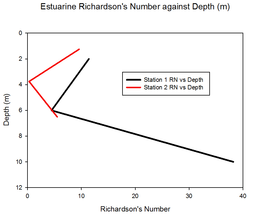
Fig. 43. Richardson number against depth
After 12 days exploring Falmouth’s inshore, offshore, estuary and pontoon a conclusion can be drawn from the data collected. A front was found offshore, near Lizzard Point (Stn 4). Phytoplankton are able to grow very well at fronts as conditions and nutrients supplied from depth by upwelling are ideal for their growth, which data from this investigation supported. Increasing proximity to the estuary’s mouth showed stratification due to mixing of sea and river waters, indicating salt-wedge characteristics. This structure appears to influence the position of the phytoplankton in the water column. The samples taken of nutrient concentrations appear to be influenced by the salt wedge as they are carried by river water. The Geophysics habitat mapping showed that the benthic habitat in the estuary was relatively homogenous, with gradations in the density of macrofauna and macroalgae; site 3 having the highest biodiversity. Sediment was coarser to the South and finer towards the North, influenced by strong tidal currents. Anthropological activity including shipping and pleasure boating all popular in Falmouth Bay would increase vertical mixing, and increase turbidity, decreasing available light and therefore alter the habitat in which the organisms live. From the head of the estuary to 20/30km offshore, changes in the biological and chemical composition are notable with considerable tidal and anthropological inputs and effects also to be considered.
![]()
Offshore:
- Barlow, R. G. 1980. The biochemical composition of phytoplankton in an upwelling region of South Africa. Journal of Experimental Marine Biology. Vol. 45 pp 85-93.
- Bouman, H. 2006. Oceanographic basis of global surface distributions of Prochloroccus ecotypes. Science 312
- INCOIS [Online] Available: www.incois.gov.in/Tutor/ShelfCoast/notes/chapter09.html [Accessed 29/06/2012]
- Garrett, G.J.R., Keeley, J.R. and Greenberg, D.A. 1978, ‘Tidal Mixing versus Thermal Stratification in the Bay of Fundy and Gulf of Maine’, Atmosphere-Ocean, 16, 403-423.
- Grasshoff, K. K. Kremling, and M. Ehrhardt. (1999) Methods of seawater analysis. 3rd ed. WIley-VCH
- Heilmann, J. P. Richardson, K. Aertebjerg, G. 1994. Annual distribution and activity of phytoplankton in the Skagerrak/Kattegat frontal region. Marine Ecology Progress Series. Vol. 112 pp 213-223.
-Holligan, P. M. Harbour, D. S. 1977. The Vertical distribution and succession of phytoplankton in the western English Channel in 1975 and 1976. Journal of Marine Biology. Vol. 57 pp 1075-1093.
- Margalef, R. 1958. Temporal succession and spatial heterogeneity in phytoplankton. University of California Press, USA.
- Johnson, K., Petty, R. L. (1983) Determination of nitrate and nitrite in seawater by flow injection analysis. Limnology and Oceanogrphy 28. 1260-1266
-Miller, Charles B. 2004, Biological Oceanography, Blackwell Publishing, Oxford, UK.
- Parsons T. R. Maita Y. and Lalli C. (1984) “ A manual of chemical and biological methods for seawater analysis” 173 p. Pergamon.
-Pingree, R. D. and Griffifths, D. K. 1978, ‘Tidal Fronts on the Shelf Seas Around the British Isles’, J. Geophys. Res., 83, 4615–4622.
- Purdie, D. 2012. Phytoplankton and Primary Production. SOES2006. Msci Marine Biology/National Oceanography Centre: University of Southampton.
- Rodriguez, F. Fernandez, E. Head, R. N. Harbour, D. S. Bratbak, G. Heldal, M. Harris, R. P. 2000. Temporal variability of viruses, bacteria, phytoplankton and zooplankton in the western English Channel of Plymouth. Journal of Marine Biology. Vol. 80 pp 575-586.
- Ross, Oliver N. and Sharples, Jonathan 2007, ‘Phytoplankton motility and the competition for nutrients in the thermocline’, Marine Ecology Progress Series, 347, 21-38.
- Sommer, F. 2002. Pelagic food web configurations at different levels of nutrient richness and their implications to the ratio of fish production: Primary production, 484, 11-20
- Taylor, J. & Ferrari, R. 2011. [Online] Geophysical research letters 38, 5 [Accessed 29/06/2012]
- Verduin, J. 2002, ‘Fronts’ , [Online]. Available: http://www.uni-hamburg.de/ihf/fronts_e.pdf [Accessed 2012 July 2nd]
- Widdicome, C. E. Eloire, D. Harbour, D. Harris, R. P. Somerfield, P. J. 2010. Long term phytoplankton community dynamics in the Western English Channel. Journal of Plankton Research. Vol. 32 (5) pp 643-655.
Geophysics and Habitat Mapping:
- Hall-Spencer, J. M., & Atkinson, R. J., 1999. ‘Upogebia deltaura (Crustacea: Thalassinidea) in the Clyde Sea maerl beds, Scotland.’ Journal of the Marine Biological Association , 79, 871-880.
- Newton. J, 2011. ‘Impacts of commercial anchoring on mearl beds in Falmouth bay.’ [Online] Avaliable: http.//www.falmouthport.co.uk/commercial/html/documents/AnchoringStudyJoeNewton.p df [accessed 02/07/2012]
Estuary:
- Ibanez, C., Pont, D. and Prat, N. 1997, ‘Characterization of the Ebre and Rhone estuaries: A basis for defining and classifying salt-wedge estuaries’, Limnology Oceanography, 42, 89-101.
- Kimmerer, Wim 2005, ‘Long-term changes in apparent uptake of silica in the San Francisco estuary’, Limnology and Oceanography, 3, 793-798.
- Marsh, T. J. and Hannaford, J. (Eds). 2008. UK Hydrometric Register. Hydrological data UK series. Centre for Ecology & Hydrology. 210 pp
- Millero, F, C. Chen, A Bradshaw, and K. Schleicher, 1980: A new high pressure equation of state for seawater, Deep Sea Research, Part A, 27, 255-264.
- Ross, Oliver N. 2006, ‘Particles in motion: How turbulence affects plankton sedimentation from an oceanic mixed layer’ , Geophysical Research Letters, 33, 1-5.

Disclaimer:
The views and opinions expressed in this site are those of the individual students and not necessarily those of The University of Southampton or The National Oceanography Centre.
![]()