
|


Introduction
Aim
Over the 9 day field course, we had an opportunity to study the biological, chemical, and physical aspects of the Fal estuary and surrounding coastal waters, utilising a variety of different scientific methods and equipment. This would provide a broad and detailed picture of the processes occurring within the estuary and offshore. The investigation will provide a range of data that will be analysed with the intention of producing a detailed scientific report. Among other things, we will be looking in particular at benthic habitats, trying to build up a picture of the range and position of different habitats within the estuary, and the behaviour of chemical constituents and physical attributes of the water along the length of the estuary and out to sea.
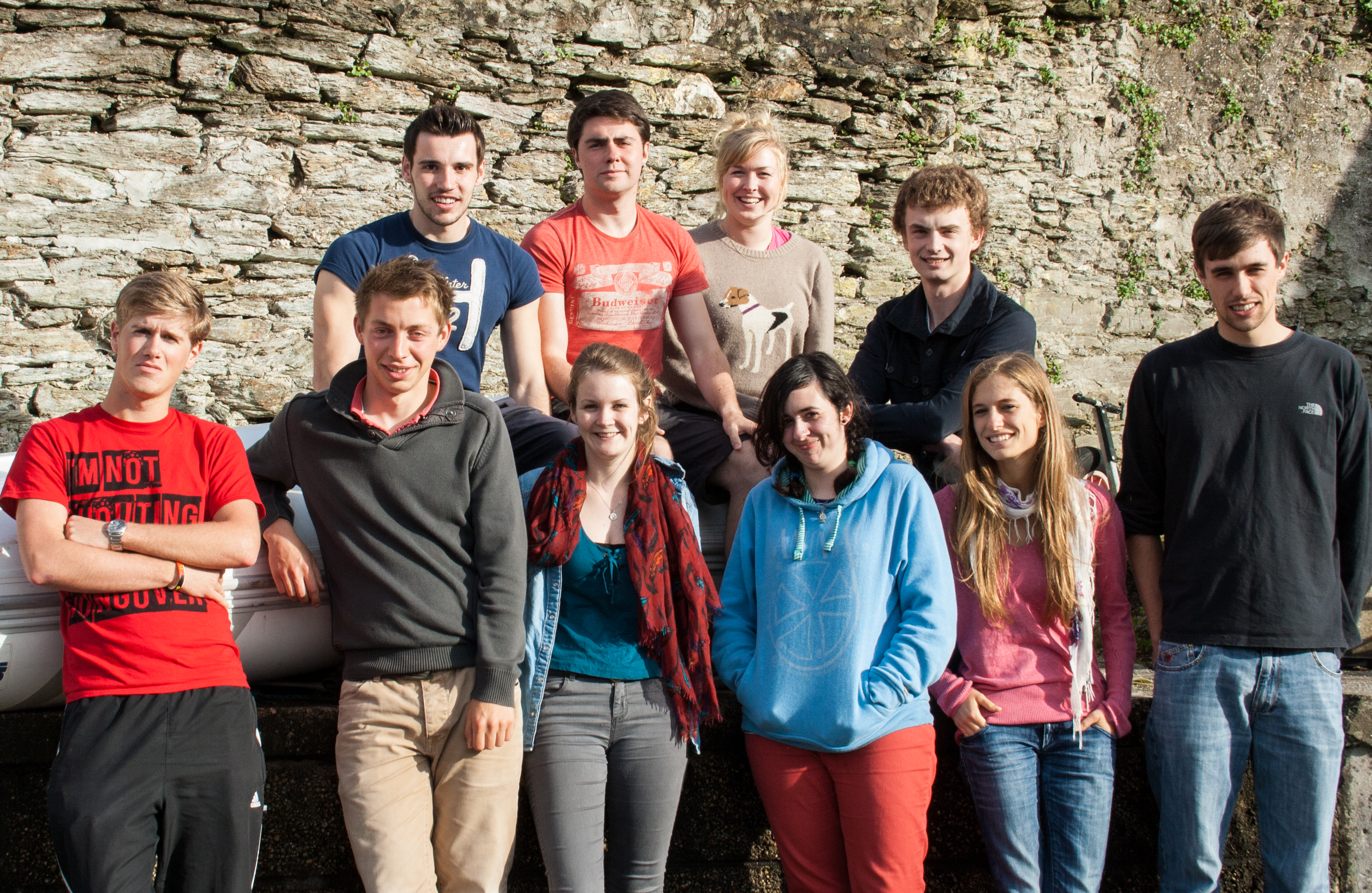
The TeamOur team was made up of 10 second year students from the University of southampton, from Marine Biology and Oceanography undergraduate programs.
|
 |
||||||||||||
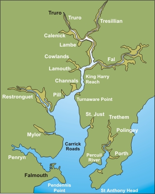 |
The AreaFalmouth is situated in the South coast of Cornwall, South-west England, and is the third largest natural harbour in the world. In the Middle Ages it was a small unimportant fishing village. Throughout the years it was considered a well situated, safe and sheltered town for vessels on trade routes to stop for repair and shelter. The major turning points in Falmouth’s gaining prosperity were the introduction of the Post Office Packet Station, which gave rise to the "Falmouth Golden Age", and the construction of the docks in 1859. Falmouth has been known through time for its mild all year round climate, with frost and snow being a rarity. |
The Fal Estuary is the third largest estuary in England, which extends from the entrance at Pendennis Point and St Antony Head to its tidal limit at Tresillian (18km inland), and the ria’s deep water channel winds further upstream to Truro. This is a product of the low sea level in the last ice age. Oyster dredging has taken place in the estuary since the Roman times and was the locals' livelihood. A similar method of dredging is still used today, although oyster fishing is less practiced. The estuary is macrotidal which has a maximum spring tide of 5.3m at Falmouth. This tide becomes mesotidal at Truro with a maximum spring tide of 3.5m.
The Fal Estuary is important for maritime trade, tourism and conservation in terms of landscape, habitats and natural harbour species. The estuary is a typical ria, or a flooded river valley. The actual ria is called the Carrick roads, which has created the natural harbour. Many commercial boats are stored in the harbour either waiting to be scrapped or sold.
Scientifically, it is also an area of high importance with five areas across the estuary being designated as Sites of specific scientific interest (SSSI). There was an abundance of mining located along the Fal estuary; Many of which are now disused and have been designated SSSI. There have been several accidental mining events in 1992 a nearby tin mine was flooded, discharging mining waste containing many toxic heavy metals into the waterways. However a study (Bryan and Gibbs, 1983) in 1983 showed that although there are raised levels of heavy metal in the estuary waters, there is no noticable reduction in estuarine flora and fauna.
Estuarine
The investigation carried out involved recording the physical, biological and chemical parameters along the length of the estuary. The aim was to see how these parameters changed as we moved from a greater proportion of more turbulent, high saline, colder water, to an area dominated by freshwater influx. It’s clear to see the differences in the chemical, physical and biological compositions through the water column moving up the estuary.
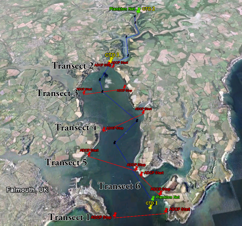
ADCP transects were conducted at the following locations and the transects are visible on this map.
Station number and name |
Transect start |
Transect end |
||||
|---|---|---|---|---|---|---|
Lattitude |
Longditude |
Time (UTC) |
Lattitude |
Longditude |
Time (UTC) |
|
Station 1 - Black Rock |
50°08.550 |
005°01.033 |
08:50 |
50°08.592 |
50°08.592 |
09.01 |
Station 3 – Truro Mouth |
50°12.334 |
005°02.324 |
12:56 |
50°12.239 |
005°02.160 |
12:59 |
Station 4 – Weir Point |
50°11.440 |
005°03.250 |
13:11 |
50°11.505 |
005°01.813 |
13:23 |
Station 5 – across from Saint Just Creek |
50°10.713 |
005°01.266 |
13:31 |
50°10.366 |
005°02.603 |
13:43 |
Station 6 – Trefusis Point |
50°09.823 |
005°03.060 |
03:53 |
50°09.402 |
005°01.701 |
14:04 |
Station 7 – St Mawes Harbour |
50°09.277 |
005°01.574 |
14:04 |
50°08.872 |
005°01.106 |
14:10 |
CTD casts were conducted at the following locations (also visible on the map)
| Station no. and name | Lat | Long | Depth (m) | Start time (UTC) |
| Station 1 – Black Rock | 50°08.571 | 005°01.618 | 19.1 | 09:11 |
| Station 1 – Black Rock | 50°08.644 | 005°01.417 | 20 | 09:21 |
| Station 2 - Pontoon | 50°14.403 | 005°00.876 | 7.5 | 11:26 |
| Station 3 – Turnaware Point | 50°12.362 | 005°02.267 | 15 | 12:31 |
Cloud cover: 8/8 octants (stratus)
Visibility: 1 nautical mile
Wind direction: 234°
Wind speed: 6.3 kn
Chemical
A total of 30 samples were taken from the estuary, from a horizontal transect, starting at Black Rock and ending at the pontoon (furthest point upstream), and three vertical profiles at Black Rock, pontoon and Turnaware Point.
The horizontal transect samples were taken using a flow through pump, and vertical profile samples were collected in Niskin bottles attached to a rosette on the CTD.
25ml from each sample were filtered to remove phytoplankton and other suspended particulates, and then put into a plastic bottle to be analysed for silicon. Another 25ml were filtered into a glass bottle to be analysed for nitrate and phosphate.
The two filters were removed and placed in 6ml of acetone to preserve them for lab analysis of the chlorophyll concentration,
In addition to this, the samples collected in the Niskin bottles were prepared for analysis of dissolved oxygen. Two Winkler's reagents (1ml of each) were immediately added to prevent biological removal of the oxygen. The bottles were then sealed and submerged in water to prevent exchange of oxygen with the air.
The methods used to analyse these variables in the laboratory are outlined by Parson et al. (1984). A modification made to this method, for silicon, was the creation of additional reducing agent to ensure that any losses were compensated for. Phosphate was modified so that blanks were only half filled at 5ml instead of 10ml, so two were added together to make one, instead of having three using four-fold mixing.
To measure the dissolved oxygen, bottle samples were treated with 1ml of sulphuric acid to dissolve the oxygen precipitate. The samples were then placed in a transmissometer with a magnetic widget to ensure the samples were mixed properly. This allowed the level of irradiance penetrating through the sample to be detected. Sodium thiosulphate was then titrated at a high resolution level (up to 0.005ml) into the sample until irradiance peaked. The results were then used to determine the percentage of dissolved oxygen in the water. The method used is outlined by Grasshoff et al. (1999).
Chlorophyll concentrations were measured with a fluorometer; using the fluorescent properties of chlorophyll pigments, the concentration of chlorophyll could be measured in the sample, giving an indication of photosynthetic activity within the water column, a method outlined in Parson et al. (1984).
Phosphate (Fig.1)Phosphate levels decrease along the estuary, from the riverine end member to the marine end member. At Site 2 and Site 3 phosphate is highest at the surface, with the highest values occurring in the surface waters at the top of the estuary (Site 2) of 0.75μmol/L. Site 1 was at the seaward end of the estuary so the riverine input of phosphate at the surface is not as high as at the other two sites. Instead the phosphate maximum occurs at 20m depth. |
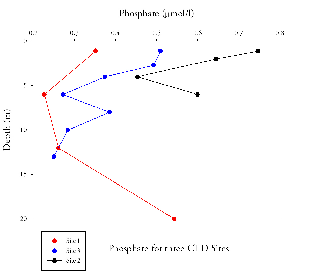
Fig.1. Phosphate samples from the length of the estuary. Click image to enlarge. |
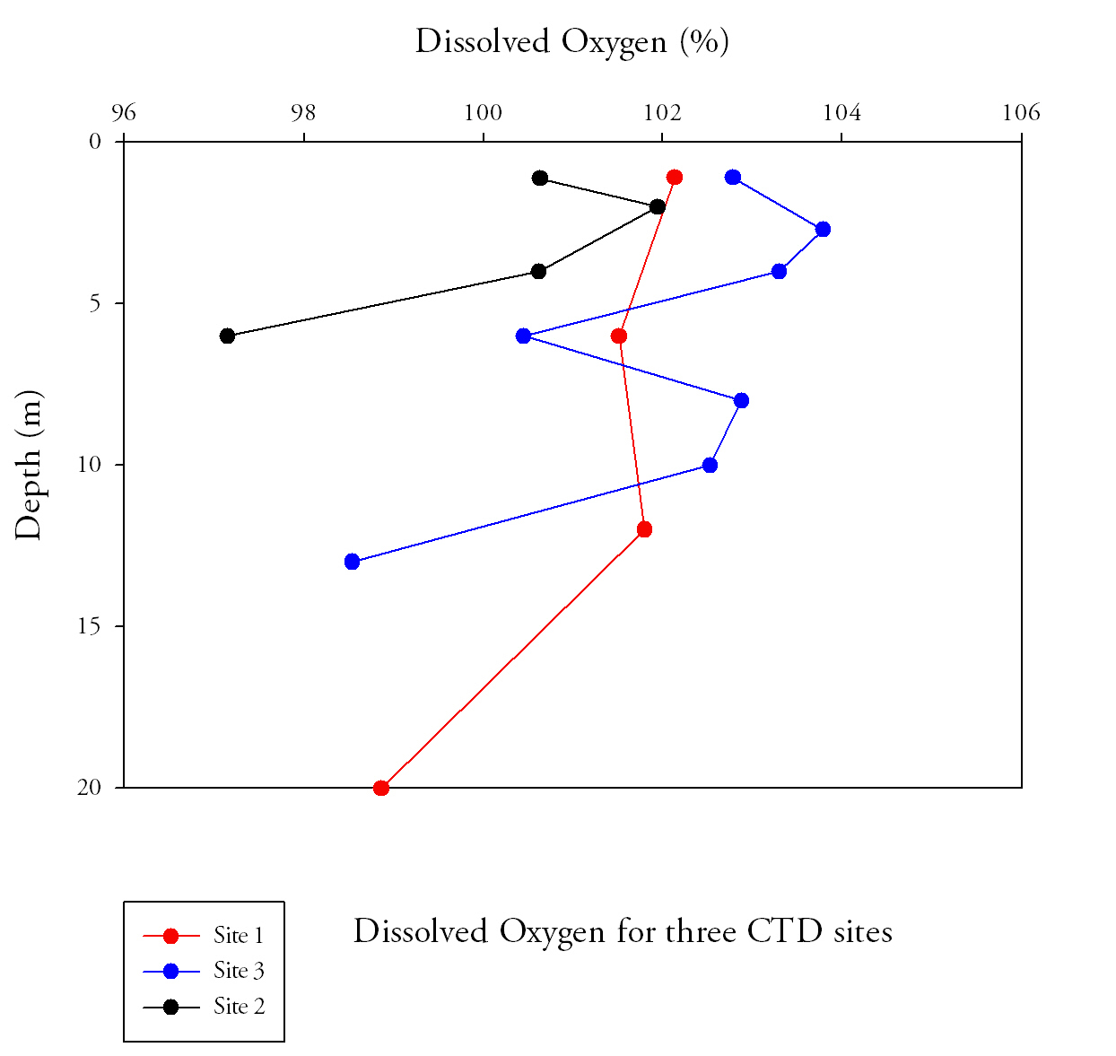
Fig.2. Dissolved oxygen samples from the length of the estuary. Click to enlarge |
Dissolved oxygen (Fig.2.)
|
Silicon (Fig.3.)Silicon concentrations are highest at site 2, with the greatest value of 8.9μmol/l found furthest upstream. Values then decrease with distance downstream and the lowest concentration of 1.1μmol/litre found at site 1. Within upper section of the water column (top 4 metres for sites 2 and 3 and top 6 metres for site 1) silicon concentration decreases, this decrease continues at site 3 until the greatest depth at 13m to a value of (2.9μmol/l). This vertical decrease is greatest at site 2 (6.6μmol/l) and smallest (0.4μmol/l) at site 1 with an intermediate value (4.2μmol/l) at site 3. For sites 1 and 2, silicon increases after the initial decrease between depths of 4m to 6m for site 2 and 6m to 12m for site 1. The greatest range of values with depth is found at site 2 and smallest range at site 1. This indicates a more uniform silicon concentration with depth at the mouth compared with the point furthest upstream which displays clear differences between surface and bottom waters. |
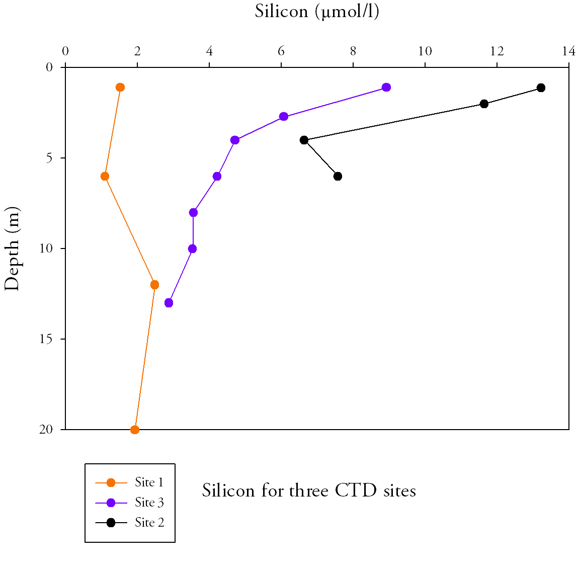
Fig.3. Silicon samples from the length of the Estuary. Click to enlarge. |
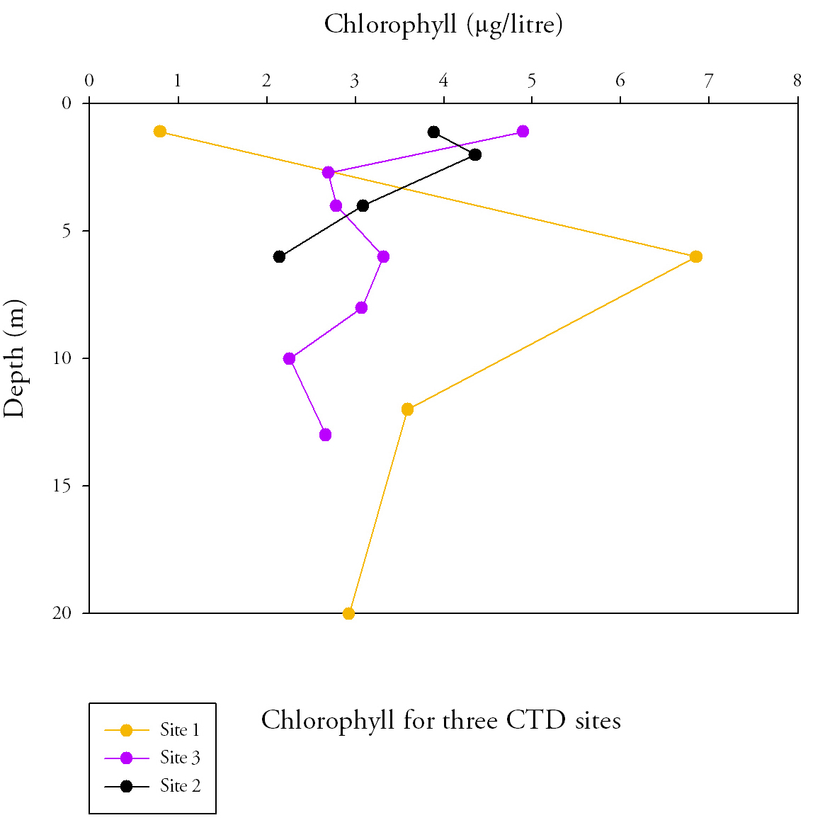
Fig.4. Chlorophyll samples from the length of the estuary. Click to enlarge. |
Chlorophyll (Fig.4.)
|
Chemical discussion
Silicon and phosphate both show a minimum concentration at depth for sites 1 and 2, and at site 3 there is also a significant decrease in concentration at the same depth. This is because at these depths the chlorophyll concentration (and therefore phytoplankton abundance) increases. Phytoplankton, in particular diatoms, use silicon to construct their frustules. When they bloom in the spring they use all the silicon in the surface river water. This is why at site 1 the silicon concentrations are very low. At sites 2 and 3 however, the silicon concentrations are high but only at the surface because the surface water contains the nutrient rich river water. They both decrease significantly with depth as the halocline in these areas prevents mixing from occurring. The increase in silicon concentration with depth may be a result of re-suspended sediment which reacts with seawater and releases silica into the overlying water column or the death of siliceous organisms from above surface waters.
Phosphate reacts in much the same way; it is required by the biota present for the synthesis of DNA and ATP in the cells. At all three sites the decrease in phosphate at depth (around 5m) can be attributed to the high concentrations of chlorophyll at the same depths. Once again, the concentration of phosphate is much lower at site 1 at the mouth of the estuary compared to sites 2 and 3 at the river end of the estuary. This is because the water column at the mouth has been depleted of nutrients from the spring bloom. The concentration has not increased since the spring bloom because of thermal stratification at the estuary mouth and the halocline at the riverine end of the estuary which prevent any significant mixing from occurring. The small increase at 20m may be because the phosphate is being added by the seawater input at the bottom of the water column, or due to re-suspension of phosphate trapped in sediments by tidal wave action.
At all three sites dissolved oxygen is highest in the surface waters. This coincides with chlorophyll, as at all three sites the chlorophyll maxima are found in the top few meters of the water column. This would indicate that the dissolved oxygen increase is because of the net photosynthesis gain at the same depth. Chlorophyll decreases with depth and therefore the amount of photosynthesis occurring will decrease. The dissolved oxygen therefore decreases as a result of this. Site 1 has a different vertical profile compared to the other two. Dissolved oxygen remains high throughout the first 10 metres in the water column. At the other two sites the dissolved oxygen decreases significantly with depth. The reason for this is because the water column at the mouth of the estuary is well mixed, there is a lack of the vertical stratification which is seen at sites 2 and 3. There is more turbulence at the air-water interface causing more oxygen to become dissolved in the surface layers. Tidal mixing and the lack of a thermocline allow this dissolved oxygen to penetrate deep into the water column.
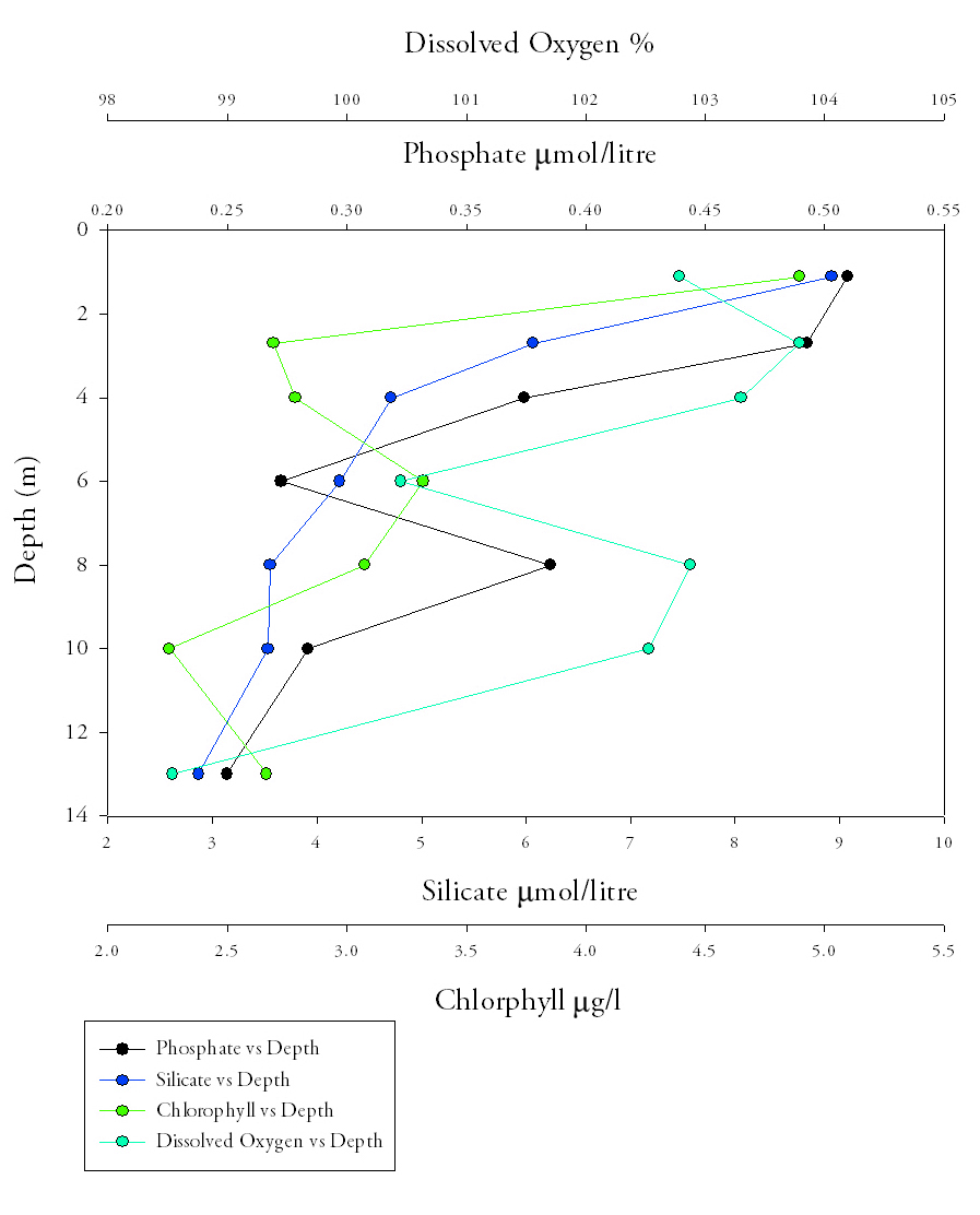
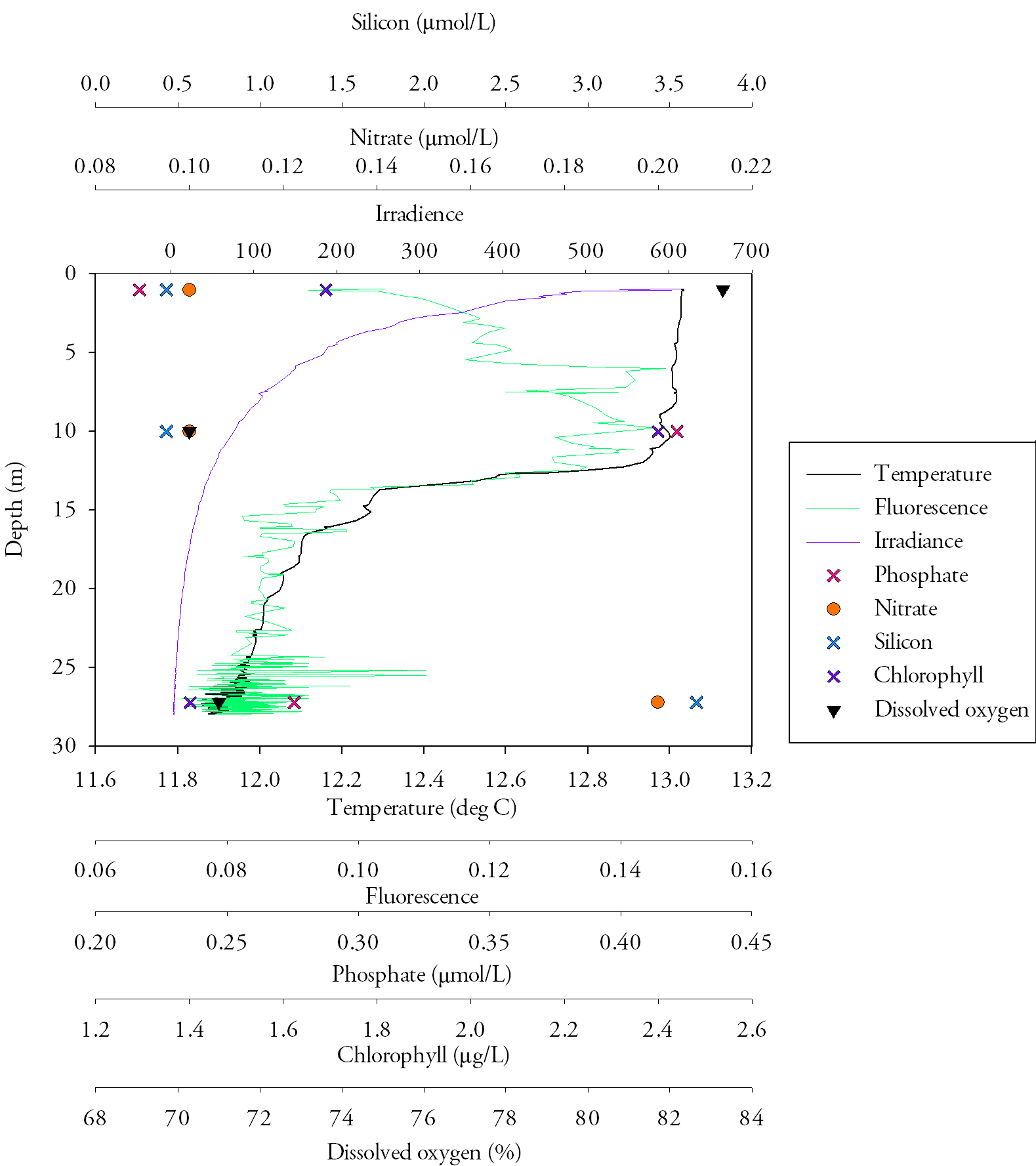
Vertical Profile AnalysisAt Turnaware Point (CTD location 3), a much higher resolution sample was taken (Fig.5.), with multiple casts taken to aquire more water bottle samples. Phosphate levels decrease with depth through the water column. At the surface the concentration is at its highest (0.5µmol/l). This decreases rapidly over the next 5m depth to 0.27µmol/l. There is then a small resurgence at 8m to 0.38µmol/l. However, after this the concentration reaches its lowest point at the bottom of the water column. Dissolved oxygen follows a very similar pattern to phosphate. It is highest in the surface waters (103.78% at 2.7m) and declines significantly over the next few metres depth (100.4% at 6m). It then increases to 102.5% at 10m in a similar pattern to phosphate. It then declines to its lowest percentage of 98.5% at 13m, the bottom of the water column. Silicate follows a simple pattern through the water column. It is highest at the surface (8.9µmol/l at 1m depth) and declines sharply over the next 5m to 4.2µmol/l at 6m, less than half the original concentration at the surface. From 6m to 13m depth the decline in concentration is steady but slow, reaching a low of 2.8µmol/l at 13m. Chlorophyll was found at its highest concentration at the surface of the water column (4.89µg/l at 1m). There is a sharp decline to 2.69µg/l at 2.7m. The concentration then increases to reach a secondary peak of 3.31µg/l at 6m. This is followed by a decline to reach its lowest concentration at 10m depth (2.25µg/l). |
Fig.5. Detailed CTD profile at Turnaware Point. Click to enlarge. |
Discussion
Chlorophyll values are at their highest in the surface waters because there is a large supply of silicon and phosphate at the surface because of the river input. Being at the surface there is also no light limitation to prevent any phytoplankton from growing. There is a sharp decline in chlorophyll values between 1 and 3 metres because of the decrease in silicon and phosphate in the water column. Light levels are also lower and therefore may be limiting growth. There is a decline in nutrient levels because of stratification occurring in the water column. Fresher and therefore less dense river water is flowing over the top of the salty and therefore denser sea water. This stratification will prevent the water column from mixing properly so once the nutrients are used by the phytoplankton they cannot be readily replenished by the river water input. In the deeper water the decline in dissolved oxygen would be as a result of the phytoplankton activity, where photosynthesis activity is lower than respiration. The chlorophyll concentration reaches its lowest point at 10m because there is not enough light penetrating to sustain phytoplankton populations so they will die off. This decline in phytoplankton population is then one reason why the nutrient concentrations increase between 6 and 10m as when they are broken down the nutrients will be released back into the water column.
CTD
A map showing the locations of all the CTD casts is available here.
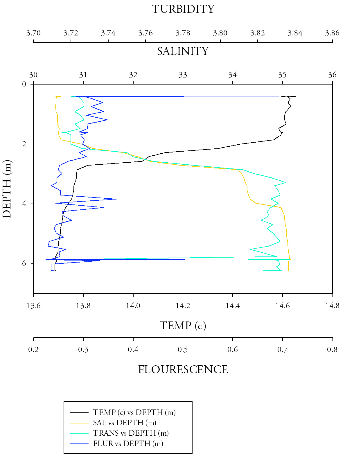
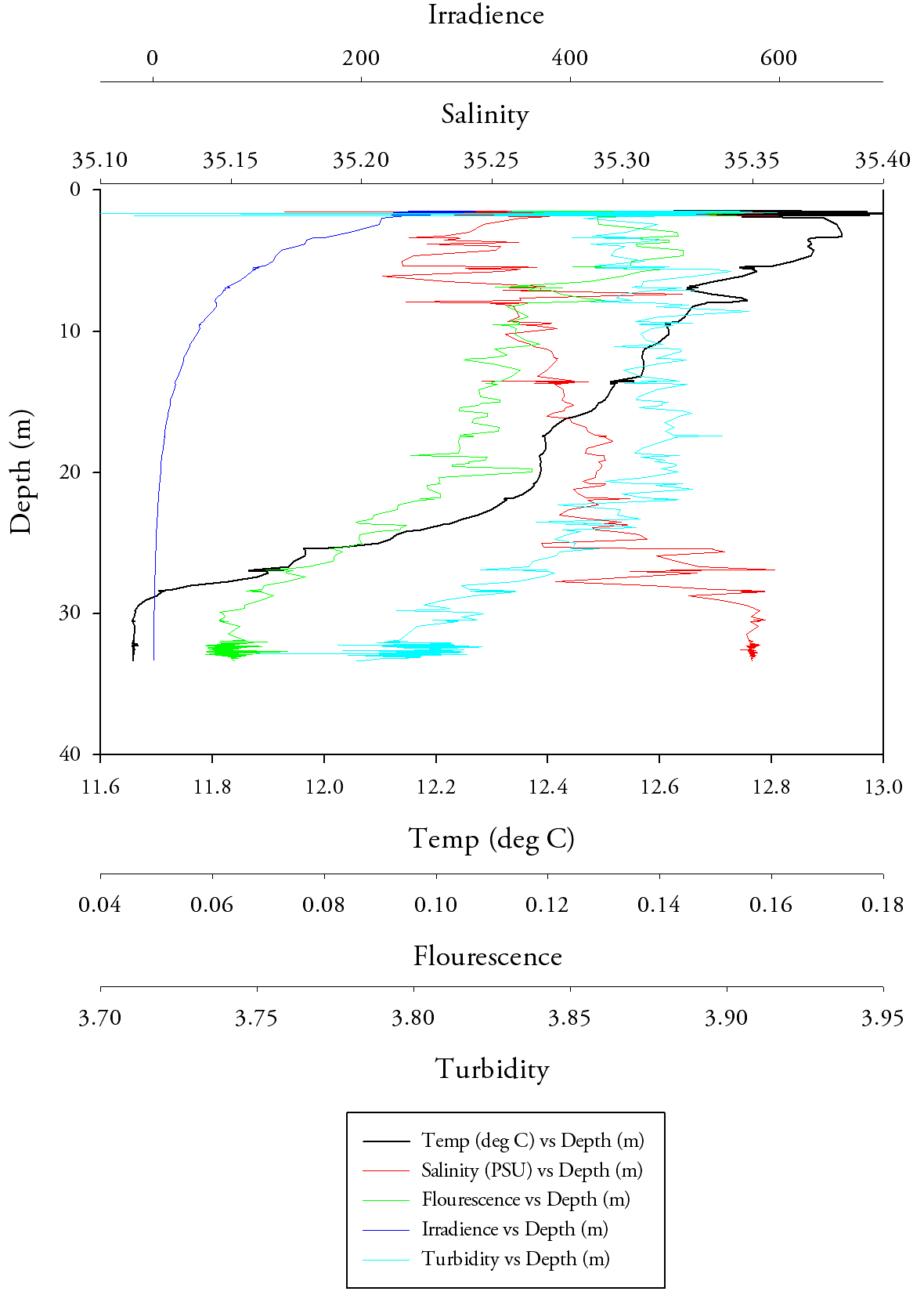
Sample site 1 (Fig.6.)Firstly, starting with temperature there is a very clear trend to notice, with increasing depth the temperature exponentially decreases. After approximately 5 metres depth the rate of decreasing temperature increases, it reaches a minimum of 12.5 at a maximum depth of 20m. The salinity data makes it clear to determine that the halocline is at around 7.5 metres, this is visible by the large increase in salinity from approximately 32.3 to 34.865 salinity units. Salinity values however are higher than would be expected even over the change with depth, this could indicate a calibration issue and problems of fouling with a sensitive piece of equipment. The transmissometer data, showing turbidity throughout the water column shows an initial decrease in turbidity (from approximately 4 to 3.97), after this event the data begins to flatten out reaching approximately 3.99 at 20 metres. Finally the fluorescence data, albeit it having several outlying results (of 0.656, 0.841 and 0.496 respectively), shows a uniform value (with an average value of 0.268). These findings show the well mixed water column. |
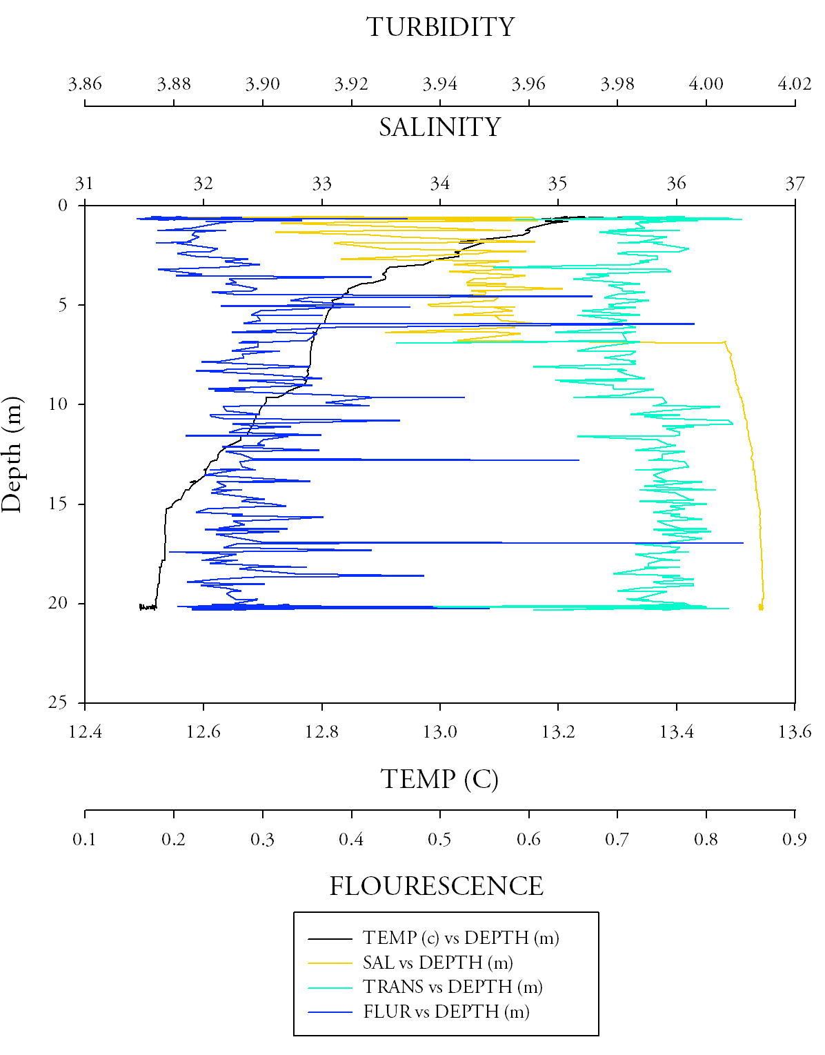
Fig.6. CTD data from the first CTD sample at black rock. click to enlarge. |
Fig.7. CTD data from the second CTD sample at the top of the estuary. Click to enlarge. |
Sample site 2 (Fig.7)Temperature in this graph follows the same trend as that from the first site, however, the average temperature (14.04) is greater; due to the fact that these results were taken from a shallower depth. At this site the salinity data shows a much smoother profile ranging from around 28.975 PSU to a maximum of approximately 33.25 at a maximum depth of 6.24m. The turbidity data also shows a much smoother distribution on the graph and between the depth range of 2 and 3m the turbidity data follows nearly the exact same pattern as the salinity. The low salinities in this area are obviously attributed to this data set being the river-end member. There is a small spike in the fluorescence data below the thermocline; this is again to be attributed to the higher levels of nutrients at this point. There is also a turbidity maximum at the base of the thermocline, this will aid phytoplankton growth by bringing up bottom layer nutrients into the sub surface chlorophyll maximum (Vidussi et. Al. 2001), however, due to this growth and therefore the incurring increase in turbidity light will become the limiting factor for phytoplankton photosynthesis. |
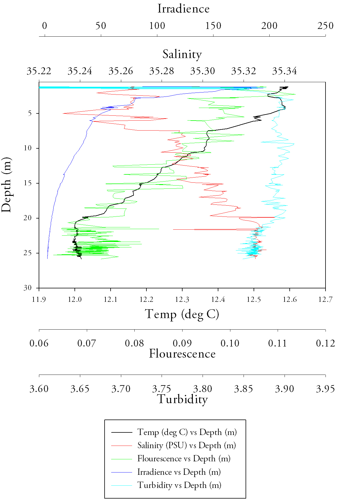
Sample site 3 (Fig.8.)Once again the temperature readings follow that of sites 1 and 2 with a peak of 14.425 at the surface and a minima of 12.14 at a maximum depth of 13.149. Like site 2 the salinity and the turbidity follow approximately the same pattern; exponential decay with depth. The consistency of the fluorescence measurements is most apparent at this site as most values lie around 0.2; however, a large outlier of 2.043 brings the overall average up to 0.269. The fresher water on the surface is causing the top water body to have a lower density, thus causing it to stay above the dense salt water below, creating a halocline, which is apparent at around 3 metres. This, in conjunction with the presence of a thermocline, caused by less dense warm water at the surface and more dense colder water at depth, further prevents mixing In the water column, therefore overall creating stratification. |
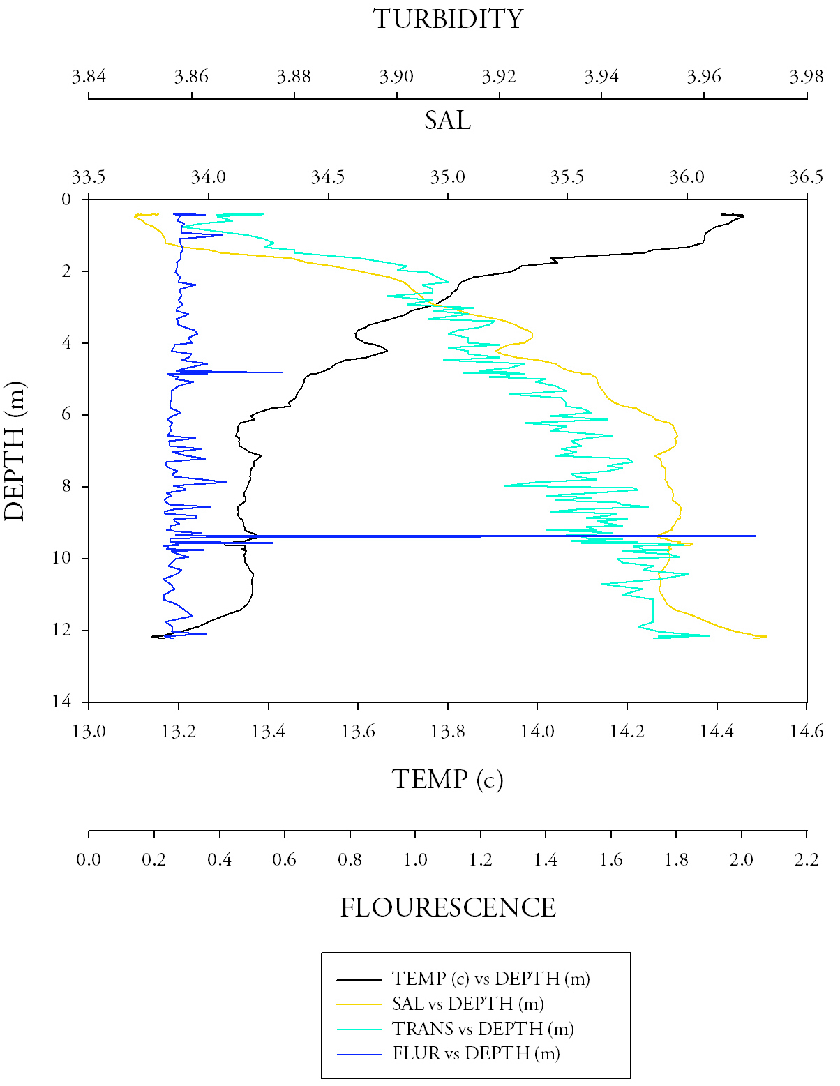 Fig.8. CTD data from the third CTD sample at the narrow section at the mouth of the Fal river. Click to enlarge. |
Theoretical Dilution lines
Fig.9. Theoretical dilution line for nitrate. Click to enlarge |
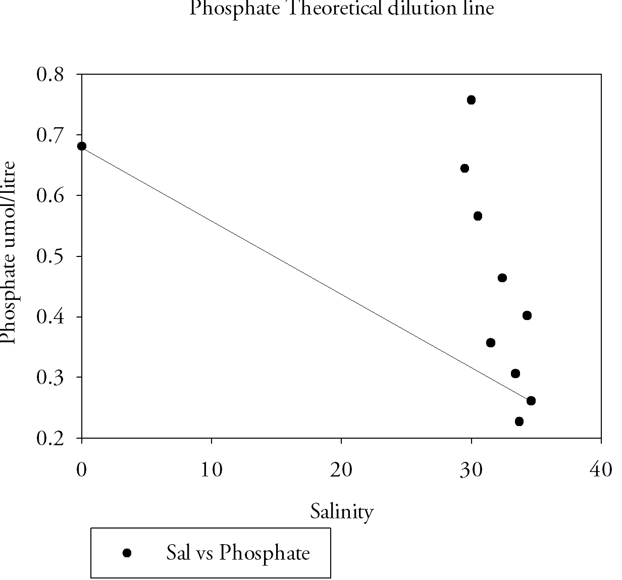
Estuarine Mixing DiagramsEstuarine mixing diagrams assume steady state for constituents, that end member concentrations are constant on a time scale greater that the residence time in the estuary and that there is only one riverine and marine end member, they are therefore affected by more rivers or waste discharge or pore waters changing composition of estuarine waters. Both Nitrate(Fig.9.) and Silicate(Fig.10) show conservative behaviour in the estuarine system changing with the salinity. Phosphate(Fig.11) shows a non-conservative behaviour. Two riverine end members were taken from Truro, the different values can be related to the different freshwater volume inputs higher at the Kenwyn and lower at the Allen. Two are taken due to the difficulty accessing the river at another suitable place. An average was taken on the mixing diagrams to meet the assumption. The seaward end member for phosphate is 0.26 µmol/l and the riverine end member 0.68 µmol/l. Phosphate levels reach 0.75 µmol/l at a salinity of 30, a higher concentration than the riverine end member. |
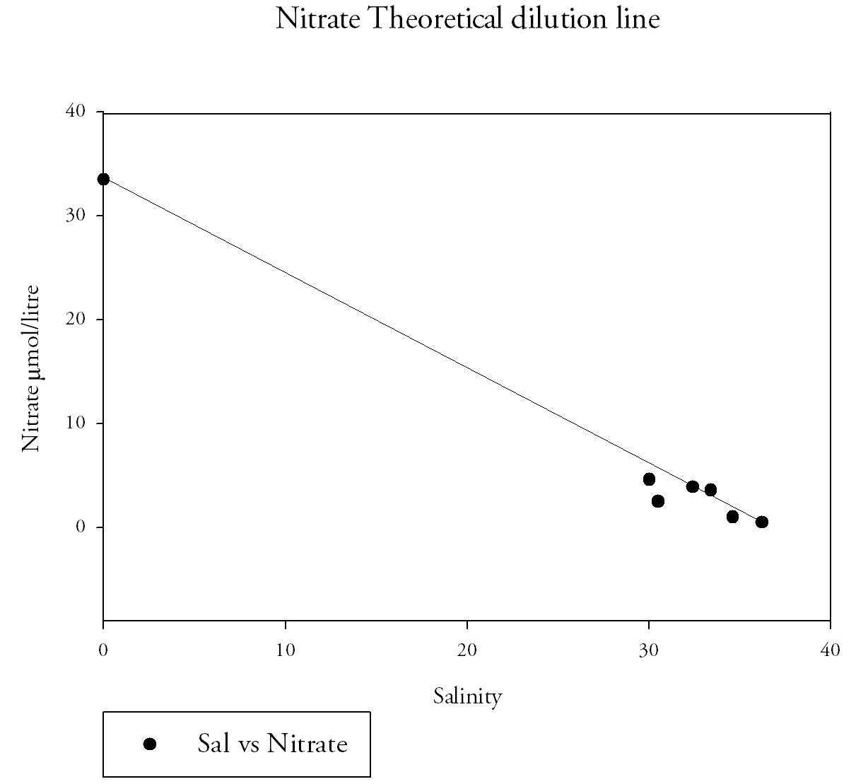
Values of 0.64 µmol/l at salinity 29.5 and 0.46 µmol/l at 32.4 are also further examples of phosphate levels that are clearly above the theoretical dilution line. The silicate river end member was 85.2 µmol/l and the seaward member was 1.3 µmol/l. The nitrate river end member was 1 µmol/litre and the seaward member was 33.5 µmol/l. It is important to remember the lab method in interpretation and the possibility of errors and difficulties in procedures. This was demonstrated in the preparation of standards the first set made was lower than expected then the second still showed variation, not always a linear increase in absorbance from concentration. There are a number of factors that may lead to a more conservative behaviour of silicon and nitrate in the estuary such as lower biological activity. Conservative behaviour relates to the mixing of seawater and freshwater which is mainly regulated by river flow rate and magnitude of tidal currents (Hansen and Rattray, 1966). A short transit time of the fresh water component of the estuary from mouth to source, leads to lower removal from an estuary, because uptake and sinking are time dependent. The transit time in the Fal estuary is high however due to the low fresh water input. Monbet (1992) found that macrotidal estuaries (tidal range greater than 2 m) such as the Fal, show a greater tolerance to nutrient pollution |
Fig.10. Silicate Theoretical dilution line. Click to enlarge. |
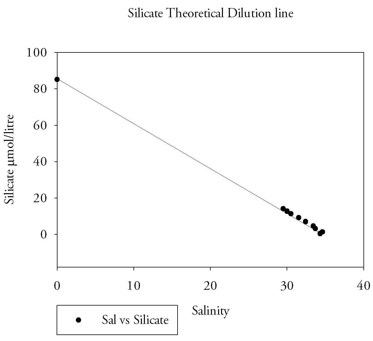
Fig.11. Phosphate theoretical dilution line. Click to enlarge |
despite high input from freshwater sources, so avoiding eutrophication. Cloern (1987) linked higher tidal mixing, current velocities, sediment resuspension, increased turbidity and decreased light penetration to lower primary productivity/biological activity and hence uptake of nutrients. Seuront and Schmitt (2005) noted that patchiness of plankton populations increases with a decrease in turbulence intensity and is higher during the ebb than during flood tide for a given turbulence intensity. This may be important in the upper Fal, where turbulence across the freshwater/seawater interface may lead to patchy distributions of phytoplankton and again lower levels of biological activity. The Fal is found in an area of extensive farming both arable and pastoral. Changes of water chemistry in the system are therefore inevitable, as observed by Jarvie et al. (2008). This could be a potential reason for the non-conservative behaviour of phosphate. Sewage treatment works at Truro and Malpas can also lead to further addition of phosphates (Langston, 2003). Mine drainage sites and sediments are also a key phosphate sources around the Fal (Langston, 2003). |
BiologicalTwo plankton samples were collected from Black Rock and pontoon. A plankton net was used for zooplankton and surface water from the flow through pump for phytoplankton. The net was deployed off of the back of the boat and was trawled for 5 minutes to collect the sample. Before deployment, the bottle attached to the end of the net was submerged to remove all air bubbles and when in the water, the rim of the net was fully submerged. At the end of the trawl, the net was washed with seawater from a hose in order to collect all zooplankton from the net. 50ml of surface water and a predetermined quantity of Lugol's iodine was added to a dark glass bottle for the phytoplankton sample. A pre-measured quantity of formalin was added to the plastic bottle collected from the plankton net for the zooplankton sample. Phytoplankton samples were concentrated from 100ml down to 10ml using a vacuum pump without removing any phytoplankton. One ml of concentrated solution was then pipetted onto a Sedgewick-Rafter chamber and five columns of twenty squares each were observed, species identified and counted under a microscope with a 10x magnification. This number was then multiplied by ten to get an estimate of the entire volume. Formalin was added to a 500ml container of the zooplankton sample to preserve organisms. From this container, each person extracted 10ml and analysed two 5ml volumes using a Bogorov tray under a microscope. The main organism groups and orders were identified and counted; the abundance per volume could then be calculated.
|
zooplankton sample as seen under light microscope, a range of different zooplankton species are present |
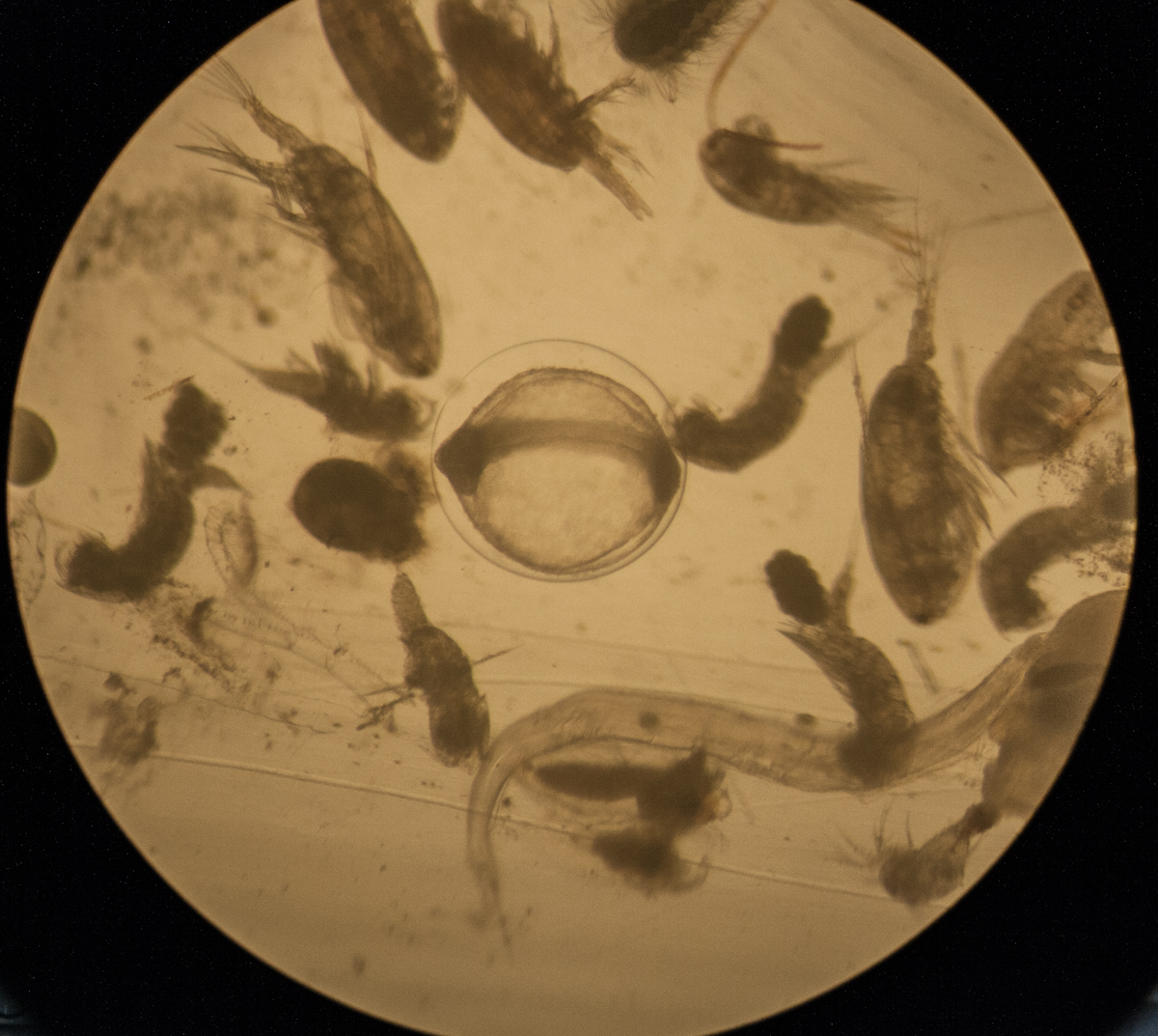
Fig.12. Phytoplankton species abundances from the estuarine stations. Click to enlarge. |
Phytoplankton (Fig.12.)
|
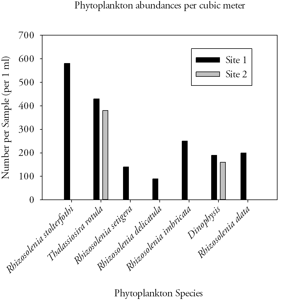
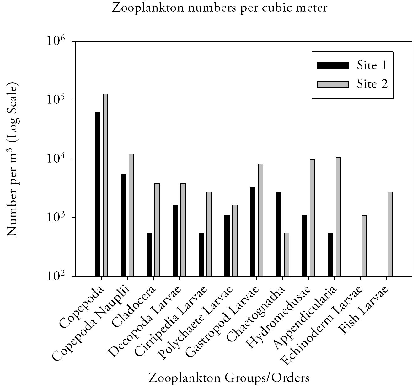
Zooplankton (Fig.13.)The range of zooplankton groups and relative abundance of each are highest at site 2, furthest upstream, except for Chaetognatha which had an abundance five times higher than at site 1. A total of ten zooplankton groups were present at site 1 and a total of twelve for site 2, with echinoderm larvae and fish larvae not present at site 1. Copepoda and Copepoda Nauplii are most dominant at both sites with relative abundances of 61600 and 5500 per m3 for site 1 and 126000 and 12000 per m3 for site 1 and 2. The least dominant species for each site differ with Cirripedia Larvae and Appendicularian for site 1 and Chaetognatha for site 2 with a relative abundance of 550 per m3 for each zooplankton group. DiscussionDiscrepancies seen for phytoplankton and zooplankton abundance between sites 1 and 2 may be explained by a variety of factors. When considering phytoplankton distribution, it is important to account for tidal state and range as phytoplankton have no or limited motility so are unable to control their position within the estuary. Sampling was undertaken in the Fal Estuary, a macrotidal estuary, on an ebbing tide, two hours after high water with a tidal range of 3.3m. |
Fig.13. Zooplankton abundances in the estuary. Click to enlarge. |
This tidal state would theoretically cause phytoplankton populations to be moved out of the estuary at the time of sampling, potentially explaining the decrease in phytoplankton abundance and range upstream. Phytoplankton populations have been shown to have increase patchiness on an ebbing tide (Seuront & Schmitt, 2005) and in areas of turbulence such as those in the upper Fal caused through the interaction between fresh and sea water (Birt, 2004).
Increased turbulence is likely to cause patchiness through vertical mixing whereby phytoplankton are mixed to greater depth. Zooplankton on the other hand are able to manipulate their position within the water column and this is of particular importance within estuaries to prevent flushing out the estuary or to transport larval stages seawards (Queiroga et al., 1997). Vertical migration is the dominant mechanism used and this is controlled by endogenous swimming activity synchronised with tidal or daily cycles; with the highest abundance of zooplankton commonly found on the flood and lowest on the ebb (Kimmerer et al., 1998). This may help to explain why a greater abundance of zooplankton species are found upstream compared to those at the mouth of the estuary.
The predator-prey relationship between zooplankton and phytoplankton species may help to explain the differences between sites. Grazing by zooplankton acts as a top-down control on phytoplankton abundance, with a surge in zooplankton abundance often occurring between May and July after the spring phytoplankton bloom, which peaks around April. When the abundance of zooplankton peaks, phytoplankton abundance is at its lowest and this may help to explain the patterns occurring furthest upstream. The greater diversity of zooplankton groups upstream may be a direct a result of increased spawning, with many organisms such as those of the benthic community releasing larvae into the water column which become temporarily become part of the zooplankton (often referred to as mesoplankton).
The species of phytoplankton found upstream at site 2, are diatom (Thalassiosira rotula) and dinoflagellate (Dinophysis) species whereas those found at site 1 were dominantly diatom (Rhizosolenia spp.) species with the same dinoflagellate species as found upstream. The presence of these species is often governed by a number of factors including nutrient availability, light penetration and species tolerances. Estuaries are extremely stressful environments and require wide tolerances especially with respect to salinity; often resulting in reduced species diversity such as that demonstrated upstream. Conditions at the mouth of the estuary are more uniform so are more likely to support a wider diversity of species.
Physical
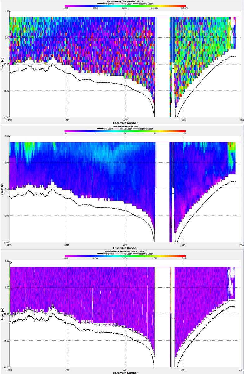
We used an Acoustic Doppler Current Profiler (ADCP) over six transects across the estuary. Looking at the velocity magnitude, direction of the flow and backscatter collectively we can make assumptions on the physical properties of the estuarine water, and oceanic offshore waters.With high velocities that flow in opposing directions there is usually a higher shear associated with the waters. This can influence the thermocline and haloclines within the water.The higher backscatter is generally thought to be higher quantities of suspended particles and as such, It can be used as a spatial representation of suspended sediment within the water column, although there are some uncertainties in this related to the current velocities (Pelletier 1988).
Over 20m the ADCP encountered problems so we were unable to get measurements in some of the deeper parts of the central channels. Map of ADCP transects
Across the estuary mouth (Fig.14.1), around Black Rock, there is a uniform velocity of around 0.2 to 0.4 ms-1, this is somewhat dependant on the tidal state of the estuary, but would be expected to be lower than other transects due to the wider and deeper cross section of the mouth. There are small elements of increased backscatter at the surface of the water column, possibly indicative of higher plankton abundances or suspended particles. The direction of flow shows distinct differences either side of the central channel with the western edge and eastern side of the channel displaying a southern flow, and the western side a north eastern flow In contrast, transect two (Fig.14.2), taken at the very narrow top part of the estuary shows an increase of velocity in the deeper parts of the channel , while the water in the shallows shows a lower velocity and a non determinate flow direction. This section also shows a greater range of velocities, from 0 to 1 meters per second. There is a large area of high back scatter in the western part of the transect, likely due to a high quantity of suspended particles in the high velocity shallower part of the channel. Transects 3 (Fig.14.3) and 4 (Fig.14.4), the mid estuary transects show similar trends, the velocity at both transects is around 0.4 ms-1, with little variance between shallower and deeper parts of the estuary, transect 3 shows an increase in backscatter above the deeper channels and transect 4 shows a minimal increase towards the west of the transect. The velocity direction in transect three is predominantly South West at the surface, however the waters nearer the bottom in the deep channel runs slightly South East reflecting the direction of the central channel. In transect 5 (Fig.14.5), the velocity direction is dominated by south-westerly flow. However towards the eastern side of the estuary flow is multidirectional, possibly caused by turbulence. Backscatter is at a minimum again along this transect. Much of the data from this transect is lost due to the failure of the ADCP over 20 meters. In transect 6 (Fig.14.6), the velocity magnitude is around 0.03-0.6ms-1 and mainly in a southwesterly direction, but with a strong flow in other directions. There is some significant backscatter in the surface layer between 1-5m which goes up to 107dB. As the transect does not cross the main body of the estuary, this transect is relatively uniform, one of the reasons why there is no deep central channel or areas of increased depth. |
|
1. Transect - 1 Fig.14. ADCP graphs for the 6 different transects, see this map for the locations of the transects throughout the estuary |
Residence Time
The residence time of the estuary can be calculated utilising the ADCP data where;
F = Flushing time (residence time)
F = fv total / R = ((1-Smean/Ssea) Vtotal)/R
Smean = Mean salinity in estuary
Ssea = Sea salinity
Vtotal = Total volume of estuary m3
R = Riverine flux m3/s
![]()
The riverine flux was taken from NERC data for the Tregony-Fal at 2.028m3/s, Kenwyn at Truro 0.378 and Kennal at Ponsmooth 0.51, averaged over the period 1978-2010. The Smean was calculated from an average of the three ctd profiles taken in the estuary. Ideally a cross sectional area could have been taken from the winriver file from appropriate transects giving the best representation of the estuary available but due to the resolution and drop out of data from the ADCP at depths greater than 20m this was not possible. The volume was therefore estimated by separating the estuary into fractions and taking average depths of the channel, adding the ADCP track length to the distance from the shore and measuring the distance between coordinates using google earth. The volume for a truncated prism was used to calculate the volume of the estuary between Blackrock and Turnaware Point. Where a2 is the cross sectional area of the smaller prism face and b2 is the larger prism face down the estuary, V = 1/3(a2 + ab + b2).
This method is an estimate and has a number of limitations and assumptions, for example it assumes that the channel depth is increasing at a steady rate between transects down the estuary, an even topography. The data for river flux is also not representative of this year where unusual patterns of rainfall have been seen. All stations used also still do not cover all freshwater inputs into the system. The area of a truncated prism does not truly represent the area of the estuary, it is an over estimate. The average depths took into account the channel as small fraction of the overall channel depth across a section.
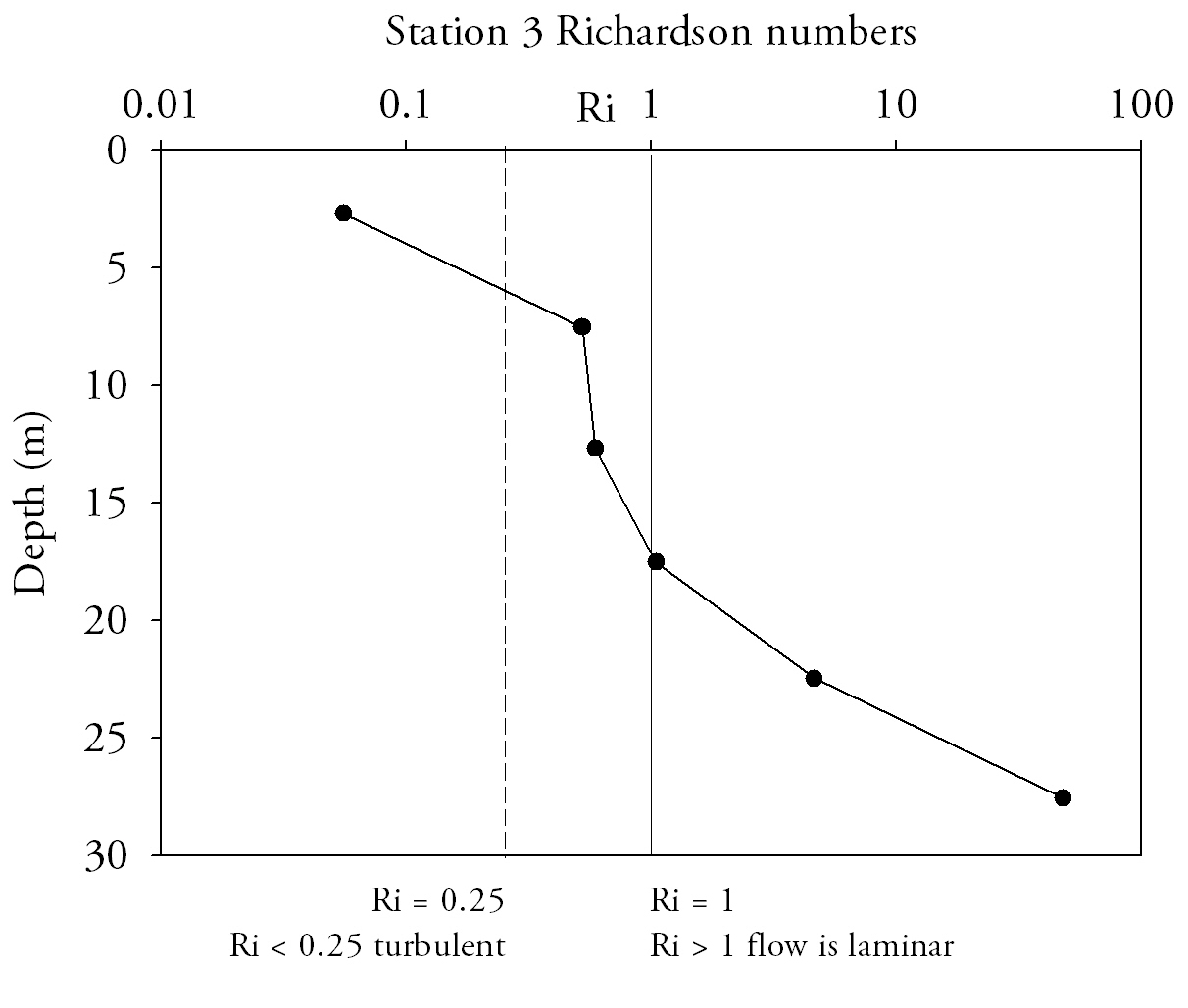
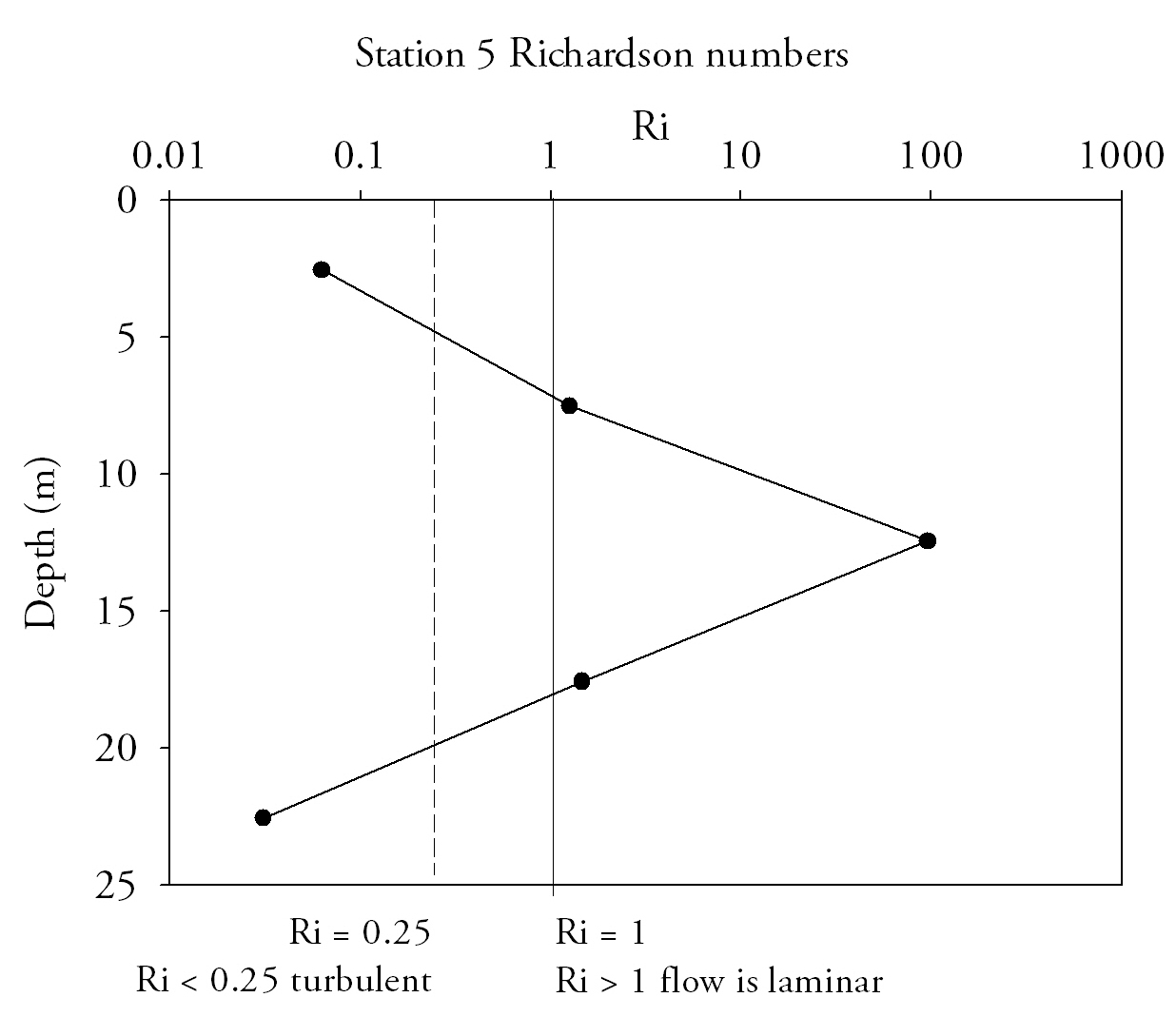
Richardson number analysis
The Richardson number (Ri) is the ratio between the density gradient (stratification) and the velocity gradient (mixing), and when Ri is high, the density gradient dominates, causing the water column to be more stable and stratified.
Where g=gravitational acceleration (ms-2), Δρ= change in density, z=depth (m), ρ=average density, u=velocity (ms-1)
When Ri<0.25 turbulent mixing occurs, Ri>1 flow is fully laminar, 0.25<Ri<1 is an area of uncertainty as could be turbulent or laminar.
Fig.15. Richardson numbers throughout the water column provide an indication of flow state, numbers below 0.25 indicate turbulent flow and above 1 indicate laminar flow. Click to enlarge. |
Richardson Numbers (Fig.15.)At the mouth of the estuary the water column is relatively stable; Richardson numbers do not decrease beneath the 0.25 turbulent threshold. Although the top two measurements are in the intermediate zone where laminar and turbulent conditions can exist, the lowest measurement has a Ri number high enough that laminar flow is definite. At Station 2 (Turnaware point), Richardson number patterns are complex throughout the water column. In the surface 4 m shear flow instability occurs as figures are below 0.25. Between 4 and 8 m there is a zone where Reynolds numbers increase through to stable laminar flow zone and peak at 3.4. Below 8 metres figures fall back below 0.25, to similar figures to that of the surface 4 metres. Richardson number patterns can be related to the data shown in ADCP plots for the same profile locations and theories deduced as to why Richardson numbers fluctuate throughout the water column. Richardson data suggest that the entire water column entering the estuary is of stable flow with Richardson number increasing with depth, and hence the stability of flow increases with depth. |
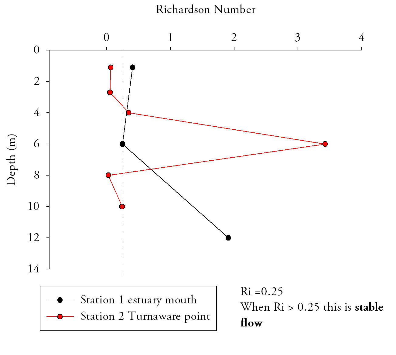
The lowest Richardson number occurs mid-water column which is mainly due to the confluence of water masses of different salinities from within the estuary and from the ocean. ADCP data from this location shows large main current flow into the estuary in the location of the CTD dip, agreeing with stable flow predictions of the Richardson number for this location.
Station 2 is in a narrow area of channel with stable current mid water column, flanked by areas of turbulent instability at the surface and at depth shown in the Richardson number plots. ADCP data shows one singular uniform direction of current flow through the water column. Areas of at the very limits of the ADCP plot at the surface and at depth are shown by reduced flow which explains why shear instability is developing in these areas of the water column.
Pontoon Time series
A time series of measurements was taken from a pontoon in the estuary to investigate how the chemical and physical characteristics changed over a tidal cycle. A YSI probe was used to measure temperature, salinity, chlorophyll a, dissolved oxygen and pH, and a light meter was used to measure irradiance. Measurements of current were expected to be taken however circumstances on the day did not allow this.
When taking light meter readings in a water column, two light meter units are used. One out of the water to measure incident light and one in the water which is lowered into the water column. Before any measurements are taken they both need to be calibrated against each other in air. Once calibration calculations have been completed on the data, you can divide the in air and in water values together to get a value between 0 and 1. Percentage attenuation can be calculated from this figure. |
Fig.30. Contour plot generated from the time series data collected at the pontoon. Click to enlarge. |
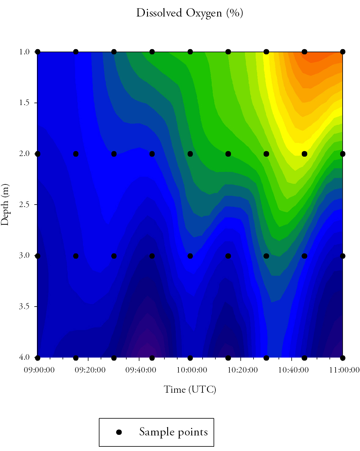
Fig.31. Contour plot generated from the chlorophyll time series data collected at the pontoon. Click to enlarge. |
Dissolved oxygen (Fig.30.)Dissolved oxygen remains low at depth throughout the time series, ranging between 95.0% and 96.0% saturation. However, the dissolved oxygen levels between the surface and 3.0m increase over time, increasing from 95.0% at 09:00 UTC, through 96.5% at 10:00 UTC, to a maximum of 97.5% at 11:00 UTC.
|
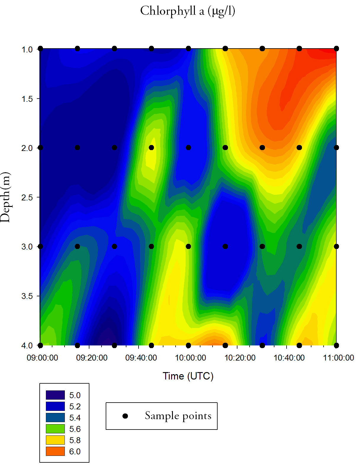
Chlorophyll a (Fig.31.)Chlorophyll is variable over time and depth, but shows an overall increase across the time series. Surface values increase from 5.0mg/L at 09:00 UTC to 6.0mg/L at 11:00 UTC. There is also a high concentration of chlorophyll a at 4m depth between 09:40 UTC and 10:20 UTC. pH (Fig.32.)pH is relatively constant over both time and depth. The water column becomes slightly more alkaline over time, increasing from 8.66-8.67 at 09:00 UTC to 8.69 at 11:00 UTC, but there is no significant pH change.
|
Fig.32. Contour plot generated from the time series ph data collected at the pontoon. Click to enlarge.
|
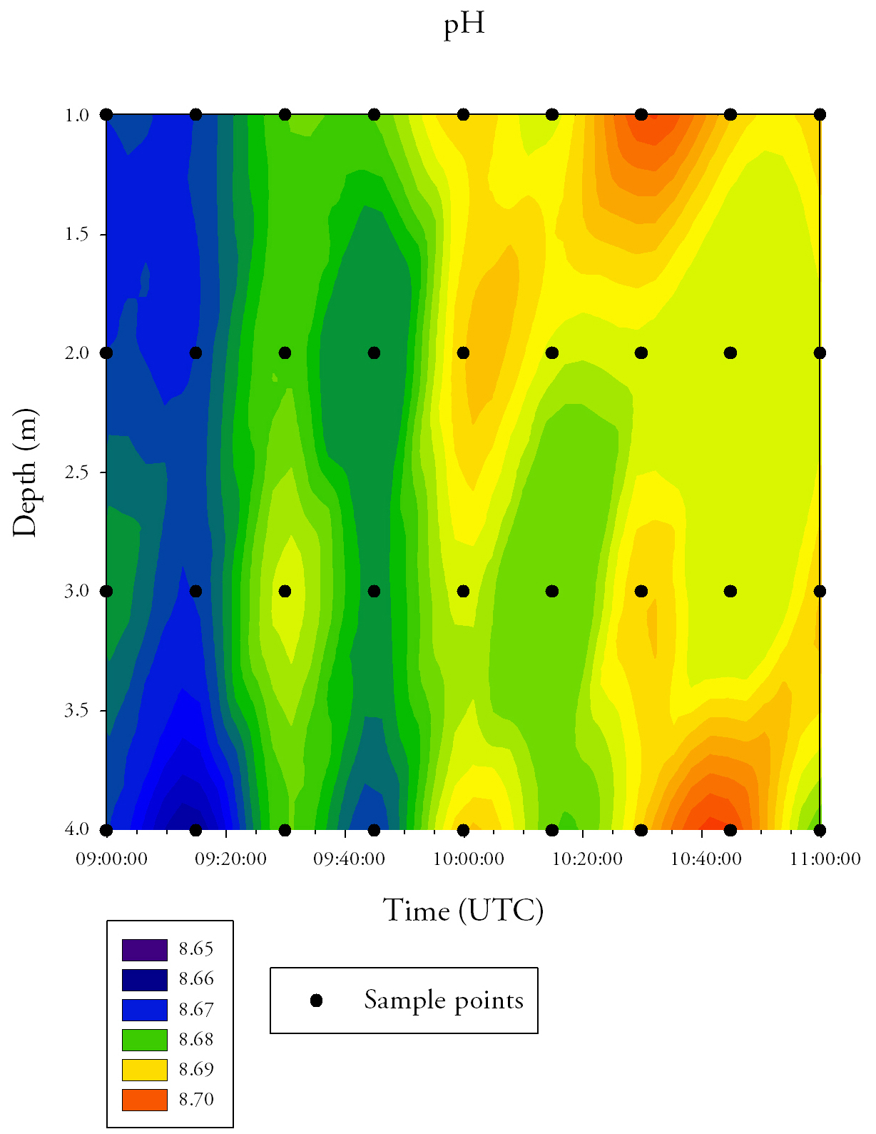
Fig.33. Contour plot generated from the time series salinity data collected at the pontoon. Click to enlarge. |
Salinity (Fig.34.)Salinity decreases across the time series, with surface salinity values starting at 32.5 and ending at 30.5. On average, salinity increases with depth; the minimum salinity at the surface is 30.5, whereas the bottom water does not reach salinities below 31.5. Temperature (Fig.34.)The average temperature of the water increases across the time series, with the surface temperature increasing from 14.6°C at 09:00 UTC to 15.2°C at 11:00 UTC. Temperature consistently decreases with depth. There is an area of cool water (13.8°C) that occurs at 3.5-4.0m depth between 10:05 UTC to 10:25 UTC.
|
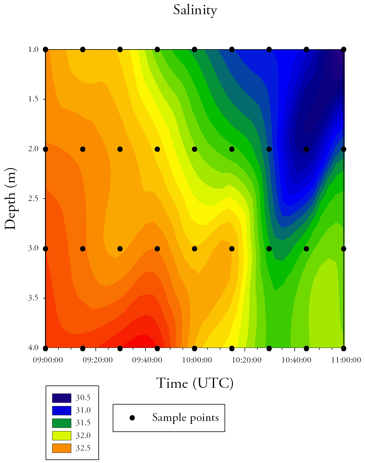
DiscussionThe time series measurements taken at the pontoon were taken at the start of the ebb tide, when the riverine input was low but its influence increased towards the end of the time series. This means that there was a significant input of freshwater at the surface. This caused the decrease in salinity over time in the surface waters and, being less dense it flowed over the more dense salt water as the tide ebbed. This also explains the temperature increase as the temperature of the ocean is lower than that of the freshwater inputs. The increase in chlorophyll a, with time, is a proxy for an increase in phytoplankton. The input of nutrients from terrestrial and riverine sources could account for the increase in chlorophyll a with time. The phytoplankton will photosynthesise, causing the increase in dissolved oxygen at the surface. |
Fig.34. Contour plot generated from the time series temperature data collected at the pontoon. Click to enlarge. |
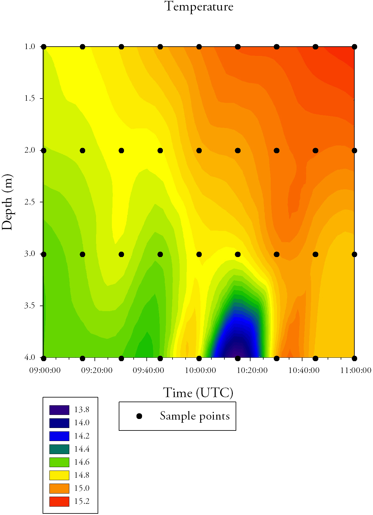
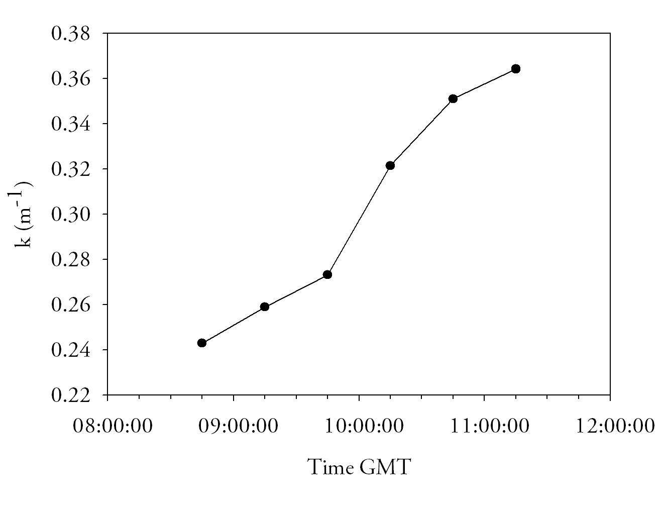
Fig.39. light attenuation time series from the pontoon. click to enlarge |
Light attenuationAt 08:45GMT attenuation is at its lowest (0.24). This increases steadily to reach a peak of 0.36 by 11:15GMT. Percentage Light levels show an exponential decrease with depth as it rapidly attenuated by water and suspended particles within it. Over time the general trend shown is that attenuation increases. One reason for this trend could be due to the tide. At 08:45 the tide is turning and is therefore still in slack water. The amount of suspended particulate matter will therefore decrease as the water has less energy to keep it suspended, hence the high levels of irradiance at this time. By 11:15, at the end of the time series, the ebbing tide is in full flow, it will therefore be carrying more particulate matter. This increase in particulate matter suspended in the water may have caused the decrease in irradiance through the water column.
|
Offshore Work
Discrete (point sample) ADCP measurements were taken at the following locations and ADCP transect measurements were carried out between these stations. A map of station locations is available here.
| Site no. and name | Start | ||
| Lat | Long | Time(UTC) | |
| Station 1 – Black Rock | 50°08.727 | 005°01.536 | 12:36 |
| Station 2 | 50°10.198 | 004°56.140 | 13:52 |
| Station 3 | 50°11.959 | 004°50.715 | 14:45 |
| Station 4 | 50°12.497 | 004°47.846 | 15:23 |
| Station 5 | 50°13.431 | 004°47.176 | 15:47 |
CTD casts were conducted at the following locations
| Site no. and name | Lat | Long | Depth (m) | Start time (UTC) |
| Station 1 – Black Rock | 50°08.727 | 005°01.536 | 30 | 12:36 |
| Station 2 | 50°10.198 | 004°56.140 | 22 | 13:53 |
| Station 3 | 50°11.959 | 004°50.715 | 32 | 14:45 |
| Station 4 – Headland | ||||
| Station 5 – After headland | 50°13.431 | 004°47.176 | 23 | 15:47 |
Cloud cover: 8/8 octants
Visibility: <1 nautical mile
Wind direction: SSW
Wind speed: 12 kn
Biological
The procedures and practices used during the offshore work were similar to the estuarine boat work, as discussed above, with a few important differences. For the phytoplankton and zooplankton samples, instead of a trawl net being towed behind the vessel for a period of time, a closing plankton net was used for a target sample between specific depths. This could be used to try and sample plankton at and just above the thermocline, where the highest plankton abundances are expected to be.
Station 1 (fig.16.)At station 1 there was a small range of phytoplankton species found. Quinardia delicatula was the dominant species and accounted for 30cells out of the 70cells per ml in total with only three species were found at the surface. At 24m only four species were identified in the water sample. These was dominated by Rhizosolenia imbricate and Guinardia flaccida which accounted for 90 and 120 cells per ml respectively out of a total of 240cells per ml. |
Fig.16. Phytoplankton abundances from the offshore sample station 1. Click to enlarge. |
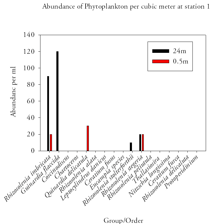
Fig.36. Phytoplankton abundances at station 2. Click to enlarge. |
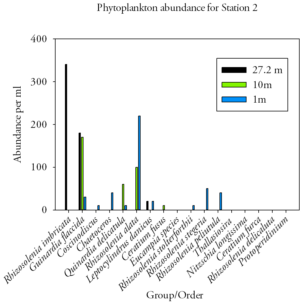
Station 2 (Fig.36.)In the surface waters at station 2 there was a large range of phytoplankton species (9 in total) which combined accounted for an average of 430cells per ml. The dominant species was Rhizosolenia alata which accounted for 220cells per ml. At 10m the type of species changed with Guinardia flaccida the dominant species with 170cells per ml. The total cell count per ml dropped to 340cells per ml with only four species present. The biota changed once more at 27m with Rhizosolenia imbricate becoming the dominant species found with 340cells per ml out of a total of 540cells per ml. The range of species declined further to three species. |
Station 3Station 3 showed a large variety of species and abundance at various depths. At the surface a total of 7 species were identified and accounted for a total of 440cells per ml. the dominant species found was Guinardia flaccida which accounted for 130cells per ml. At 19m depth a total of 8 species of phytoplankton were identified. The dominant species was Rhizosolenia stolterforthii which had a total of 160cells per ml. Two species to note that were identified were Nitzschia longissima and Ceratium furca but were found in low abundance (10cells per ml). The total abundance of phytoplankton cells at 19m was 430cells per ml. The range of species found at 32m decreased to seven. The dominant species was Guinardia flaccida which had an abundance of 110cells per ml. The total abundance of phytoplankton found at 32m was 270cells per ml. |
Fig.37. Phytoplankton abundances at station 3. Click to enlarge. |
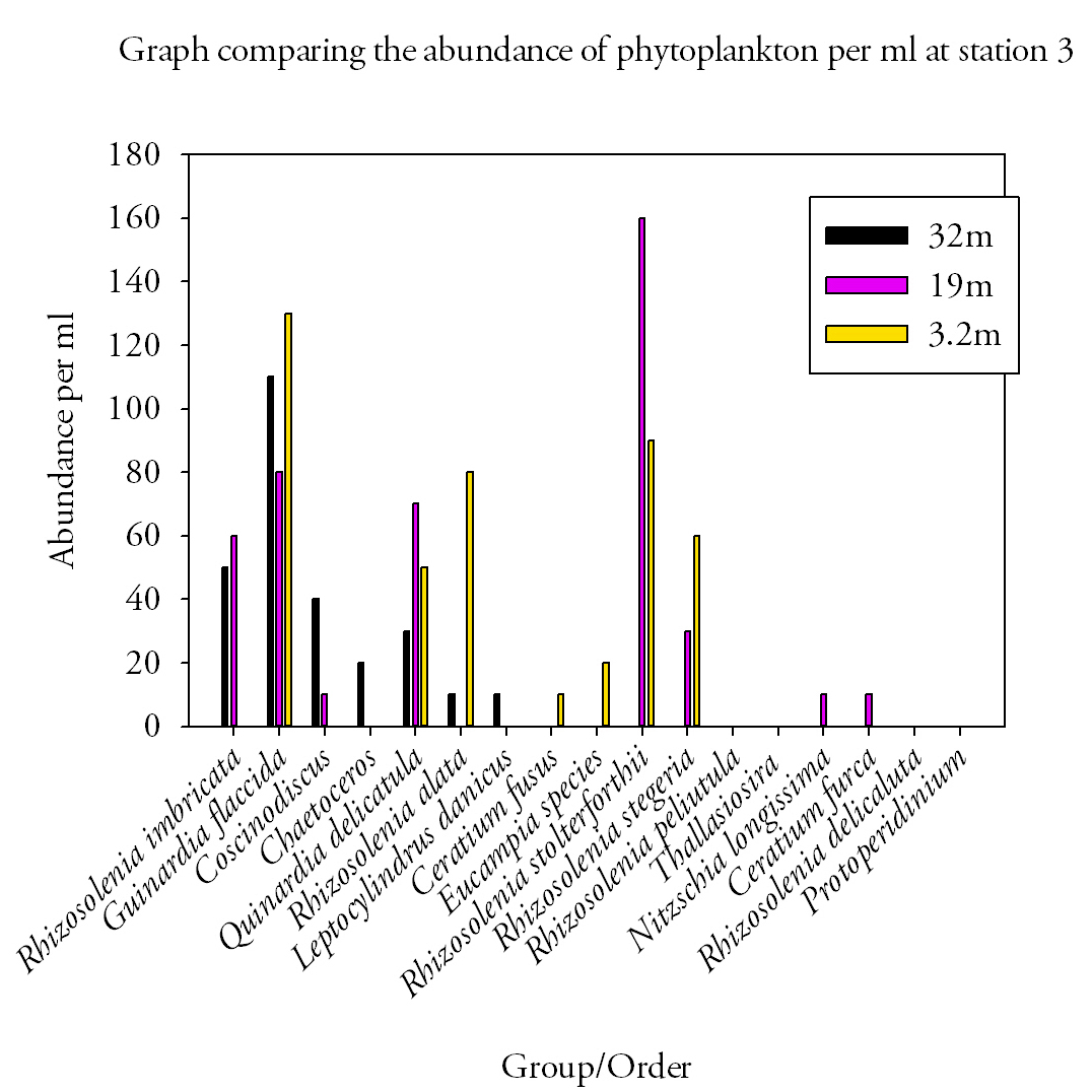
Fig.38. Phytoplankton abundances at station 5. Click to enlarge. |
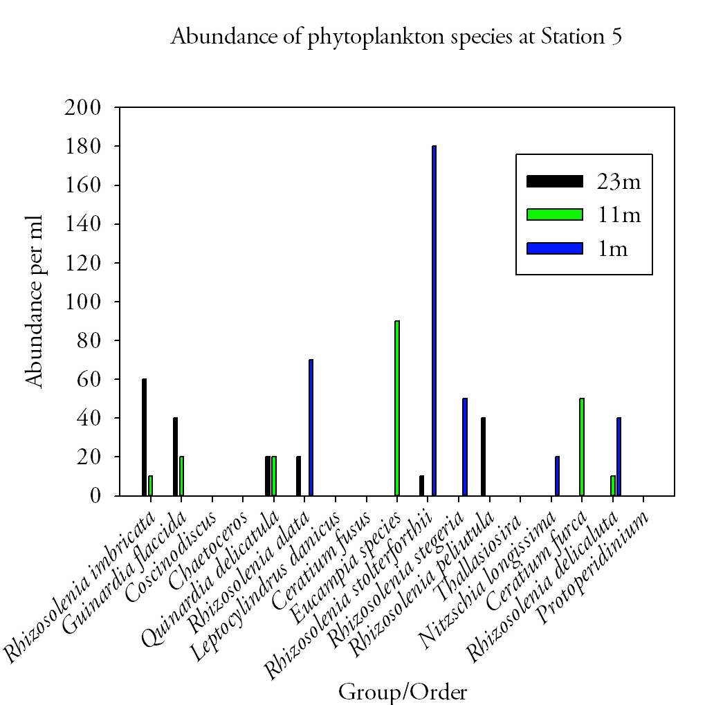
Station 5Five species of phytoplankton were found at the surface at station 5. The dominant species was Rhizosolenia stolterforthii which had an abundance of 180cells per ml. All five species accounted for 360cells per ml in the surface water. At 11m, six different phytoplankton species were found. The total abundance at this depth was 200cells per ml, of which the dominant species (Eucampia species) accounted for 90cells per ml. The range of species found at 23m remained at six but different species were present. They had a total abundance of 190cells per ml. The dominant species found at this depth was Rhizosolenia imbricate which had an abundance of 60cells per ml. DiscussionDiatom species dominated at all sites most notably Rhizosolenia imbricata at sites 1, 2 and 4 and Guinardia flaccida at sites 1,2 and 3. A noticeable bloom of diatoms during the summer months has been known to occur with the dominant presence of small Diatom species Rhizosolenia and Pseduo-Nitzschia recorded in the Western English Channel (Widdicombe et al., 2010). Despite this, previous findings oppose this trend including surveys conducted by Holligan and Harbour (1977) who found dinoflagellates to dominate from June to August within the thermocline. They did however observe the presence of particular diatom species to extend into June; one of which (Rhizosolenia delicata) was recorded at site 5. The presence of Diatoms towards the end of June can be explained by the occurrence of favourable conditions that are able to support the growth of larger phytoplankton species (Holligan & Harbour, 1977). |
In areas where intermediate vertical stability exists the difference in temperature between the upper and bottom layers of the water column lies between 1.0 and 3.0 °C. These conditions allow the mixing of nutrients into the upper layers allow the growth of diatoms to extend into June in cool summers (Pingree et al., 1977). At all stations the temperature difference between the top and bottom layers do not exceed 1.1°C. In addition to this, increased mixing attributed to high wind speeds (15mph), stormy weather and spring tidal state all assist in breaking down any stratification to favor conditions suitable for diatoms, who prefer turbulent environments (Holligan & Harbour, 1977). Alternatively nutrients to aid growth may be supplied into surface waters from allochthonous sources such as anthropogenic inputs from the River Fal that drain agricultural land.
Sites (3 and 5) where phytoplankton abundance is greatest in surface waters are those with the least pronounced thermocline. This lack of thermocline may create unfavourable conditions for photosynthetic phytoplankton as the formation of a stable upper layer cannot occur causing phytoplankton to be mixed below the depth at which net photosynthesis will occur (Miller, 2004). They therefore tend to reside within surface waters to take advantage of high light levels that exist there.
The distribution of vertical phytoplankton profiles is ultimately controlled by the two factors limiting phytoplankton growth. These are light intensity which decreases with depth and nutrient availability which increases with depth and the combination can result in deep chlorophyll maxima (Ryabov et al., 2006), which appear to be occurring at site 1 and 2, both that occur at depths below the thermocline. This layer is extremely variable and is dependent on species requirements, abundance and distribution (Ryabov et al., 2010). Rhizosolenia spp. and other diatoms have to found to be significant in the bottom water particularly mid-June after the spring bloom with a great diversity at 50m than 10m as a result of sinking processes from the surface waters (Holligan & Harbour, 1977). At site 3 however this is untrue with the number of species 3 times less at depth than at the surface, most probably due to the lack of species adapted to such stressful conditions giving those adapted a competitive advantage within that environment (Ryabov et al., 2010).
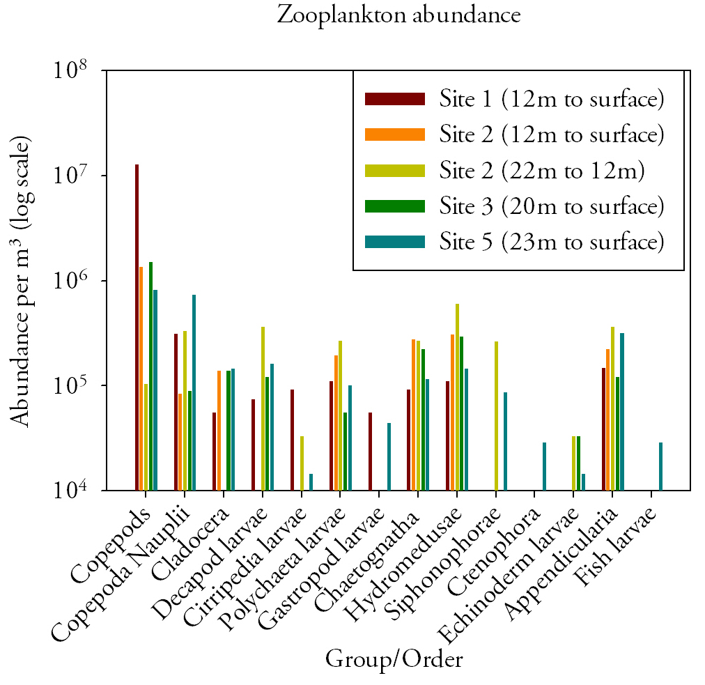
Zooplankton (Fig.17.)Copepods are dominant in site 1,3,5 and 2 (from 12m to surface), while site 2 (from 22m to 12m) is dominated by hydromedusae. Copepods, Copepod larvae, Polychaeta larvae, Chaetognatha, Hydromedusae and Appendicularia are present at all stations. Echinoderm larvae, Fish larvae, Ctenophora and Cirripedia larvae are not found at all sites and where they are present, their abundance is very low. There is a significant difference in the abundance of Copepods between station 1 (sampled from 12m to the surface) and station 2 (sampled between 22m and 12m). At station 1, Copepods are 124 times higher than at station 2, with 1.28×10⁷ m3 at station 1 and 1.03×10⁵ m3 at station 2. The abundance of Hydromedusae, is however almost 2 times greater at station 2 between 22 and 12m than it is at the same station between 12m to surface, in fact, between 22 and 12m the abundance is 5.96×10⁵ and between 12m and the surface the abundance is 3.04×10⁵. |
Fig.17. Zooplankton abundances per cubic meter from the offshore excursion. Click to enlarge. |
Discussion
Fish larvae are only present at site 5 and in low abundance (2.88×10⁴ m3), according to the Royal Commission on Environmental Pollution (2004), fish larvae feed on a specific groups of copepods, mainly C. helgolandicus and C. finmarchicus. The study states that C. helgolandicus peaks in autumn and, therefore copepods available to fish larvae are lower in summer, resulting in a lower abundance of fish larvae. Grazing by zooplankton occurs after the phytoplankton bloom during spring in temperate waters, most of the zooplankton biomass is then concentrated above the thermocline. As the season progresses, there is a reduction in the phytoplankton biomass due to grazing, leading to the vertical migration of zooplankton in deeper water below the thermocline.
The absence of different groups of zooplankton at certain sites and the low abundance of specific zooplankton types such as ctenophores seen on the graph could be attributed to seasonal vertical migration (Lalli and Parsons, 1997). A study made by Eloire et al. (2010) showed similarities in the type of food source selected by Cirripedia larvae and Copepods. The abundance of Cirripedia larvae for sites 1, 2 (22m to 12m) and site 5 is significantly lower than the abundance of copepods at the same stations, the average copepod abundance for site 1,2 and 5 is 4.57×10⁶ while the average of Cirripedia larvae at the same sites is 4.65×10⁴ suggesting that copepods outcompeted Cirripedia larvae.
Station 2 was sampled both from 22m to 12m and from 12m to the surface. On the graph it can be observed that Copepods dominates between 12m and the surface at station two, while Hydromedusae at the same station dominates between 22m and 12m. Because the thermocline at station 2 was situated at 13m, the inverse relationship between Copepods and Hydromedusae at this station implies that Copepods sit above the thermocline while Hydromedusae is situated below.
Chemical
At each station, a CTD depth profile was undertaken, with bottle samples being taken at specific depths, The onboard measurements on the CTD were used to target bottle samples at relevant depths to observe key profile features. The processing and analysis of the bottle samples was the same as the estuarine chemical analysis (above).
Vertical Profile
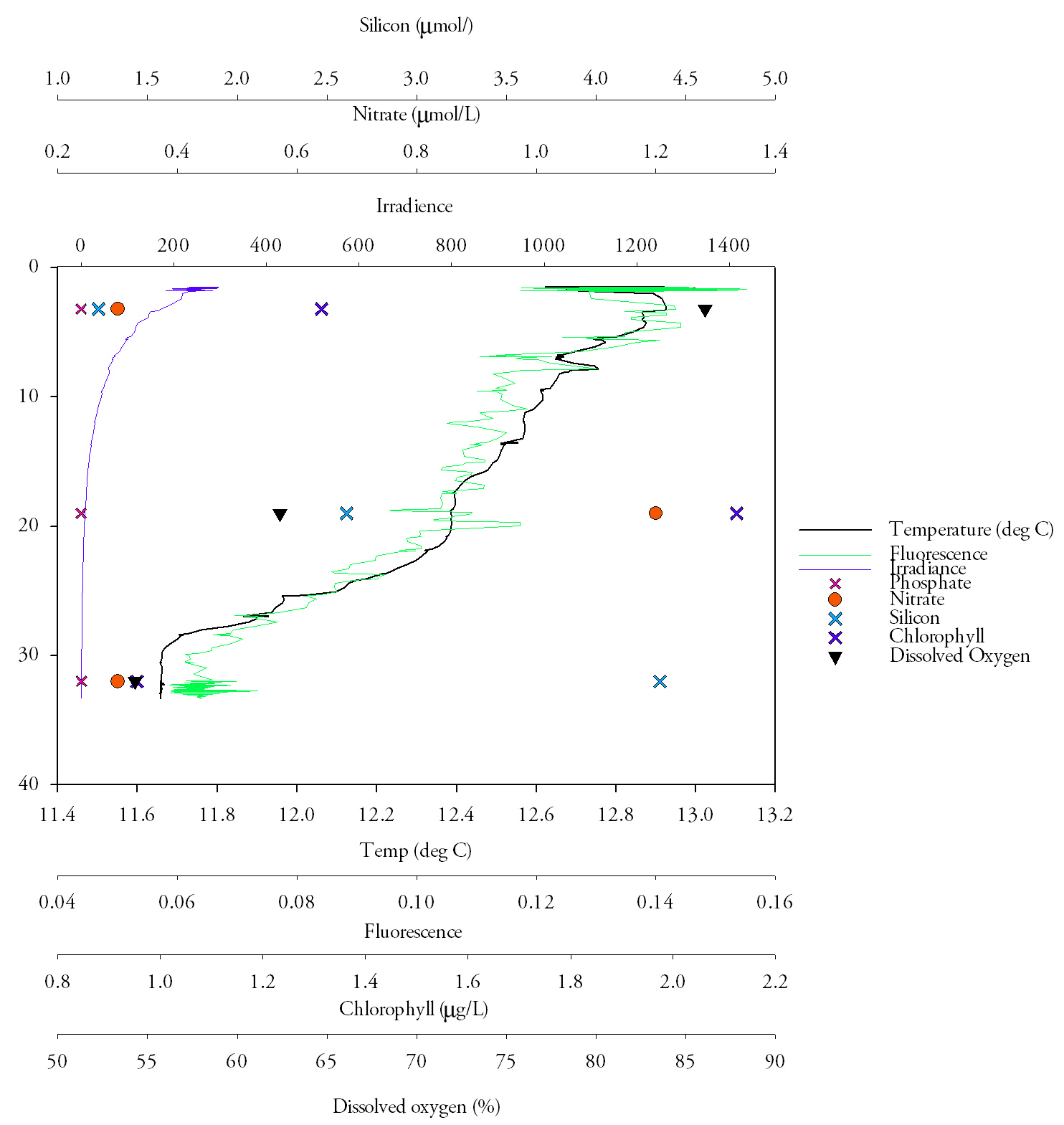
Station 2 (Fig.22.)Temperature is highest at the surface at 13.0˚C, and lowest at the bottom at 11.9˚C, with a strong thermocline at about 13.8m. The fluorescence follows the thermocline and is matched by the chlorophyll, which peaks at 2.4mg/L. Nitrate is low in the surface waters, at 0.1mmol/L, and stays low moving down through the water column, increasing to 0.2mmol/L below the thermocline. Silicon also follows this pattern, starting low at 0.43mmol/L and reaching a peak of 3.66mmol/L at 27m depth. Dissolved oxygen decreases with depth, starting at 83.3% saturation at the surface, decreasing rapidly to 70.3% at the thermocline and remaining fairly constant after that, increasing only slightly with depth to 71.0%. Nitrate does not change much with depth, but does increase slightly below the thermocline, from 0.1mmol/L to 0.2mmol/L Phosphate is depleted at the surface and bottom, and peaks at 0.42mmol/L, just above the thermocline. Irradiance decreases exponentially with depth. DiscussionThe temperature decrease from the surface to the bottom is only 1.1˚C, but this occurs over only a few metres, producing a very sharp thermocline. This shows that the water column is stratified, likely due to the solar heating that occurs during the spring. The fluorescence and chlorophyll correlate very closely, indicating that there is an increase in phytoplankton mass at about 5m, which declines again approaching the thermocline. This pattern can be explained by the nutrient values; nitrate and silicon are both depleted in the surface waters due to biological utilisation, and high in the bottom waters, below the euphotic zone. |
Fig.22. The analysed water samples from CTD casts at station 2, displayed on a depth profile with the relevant CTD data. Click to enlarge |
To compromise between the low-nutrient surface waters and the low-irradiance deeper waters, the phytoplankton live predominantly on, or near, the thermocline. Phosphate is low in the surface waters due to uptake by phytoplankton. However, it peaks at the same time as chlorophyll, where it should be depleted. This could be due to addition of phosphate to the water column by a freshwater input, or possibly an error in measurement. The high oxygen saturation at the surface could be explained by diffusion of oxygen into the water at the air-sea interface, which gets mixed into the surface layer. It then decreases rapidly as it used in respiration by phytoplankton, which are not photosynthesising efficiently due to the lack of nutrient input that results from stratification.
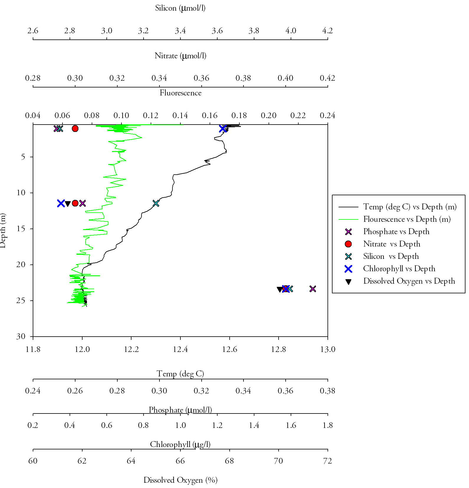
Fig.23. Water sample depth profile from station 3 with the relevant CTD cast data. Click to enlarge. |
Station 3 (Fig.23.)
|
This links dissolved oxygen to fluorescence, which also decreases with depth, and indicates a decrease in chlorophyll and therefore phytoplankton activity with depth. The increases in phosphate and silicon with depth are due to utilisation by diatoms and other phytoplankton in the euphotic zone, which does not occur at such a high rate below the euphotic zone. This also explains the lack of nitrate at the surface, but the peak in nitrate occurring at the same depth as the chlorophyll peak is unexpected. The large size of the value suggests that the peak in nitrate at this depth could be caused by an error in the lab analysis, for example contamination, or an error in the flow injection analysis set-up.
Station 5 (Fig.24.)
|
Fig.24. Water sample data depth profile with relevant CTD data. Click to enlarge. |
The lack of a thermocline may be explained by the fact that at station 5, wave size had increased as well as wind speed which may have helped create a well-mixed water column. Nitrate, phosphate and silicate are all low at the surface because of the presence of phytoplankton at the surface using up all the available nutrients. They increase with depth because of insufficient light levels that prevent phytoplankton from occurring. However, at 23m the increase in chlorophyll levels could be because of the amount of shear stress occurring in the water. The two opposing currents at station 5 caused mixing to occur throughout the water column. This therefore could have pulled phytoplankton from the surface layers to bottom layers of the water column. It would also explain why dissolved oxygen increases with depth where one would expect it to decrease. However as the data collected is discreet data it would suggest that this is not always the case. The continuous data from the CTD regarding fluorescence suggests that the bottle samples were an isolated example as it did not detect any peak in chlorophyll at 23m.
Physical
CTD casts were taken at every station apart from station 1, the CTD measured a range of physical parameters; temperature, turbidity, irradiance, salinity and fluoresence.
Due to the increased swell in the area which caused the boat to move significantly from the original sampling point a lot of unnecessary noise was observed from the CTD at site 1, thereby making a graph incredibly difficult to generate. Starting with station 2 (Fig.18.) and the temperature data, it is the same pattern that one would expect; there is a peak temperature at surface of approximately 13.0°C which stays relatively constant through to a depth of 13.0m where it then suffers a large decrease down to 12.3 at a depth of 13.8m, this is the thermocline. After the thermocline the temperature gradually decreases to 11.9°C at a depth of 27.8m. Due to this being offshore data after the first meter the salinity data is relatively constant with only a range of approximately 0.1 salinity units. However, a clear halocline is visible at 13.6m, where there is an increase from 35.1 to 35.3 salinity units. In terms of fluorescence the general trend to notice is the dramatic increase from 0.105 to 0.133 at approximately 13m (at the same place where the temperature decreases dramatically). The irradiance data shows an exponential decay with depth and an asymptotic relationship towards 0. The turbidity data shows a similar relationship as that salinity data, after the first meter the data becomes relatively constant with and average value of 3.8 and a range of approximately 0.02. |
Fig.18. CTD data depth profile from the second station. click to enlarge. |
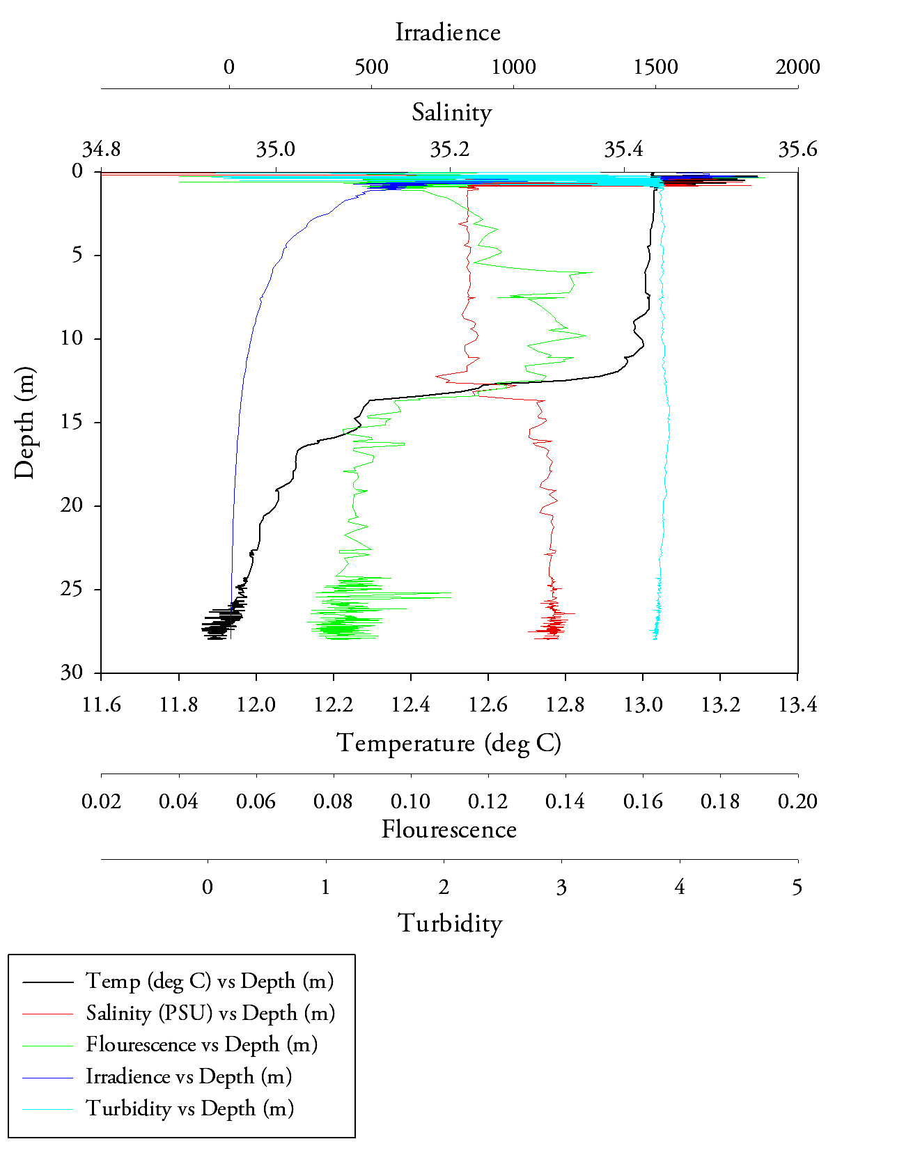
Fig.19. CTD data depth profile from the third station. Click to enlarge. |
At station 3 (Fig.19.) the thermocline is much less pronounced, however one could argue that it occurs at roughly 20m where the gradient of the temperature data is at a minimum. At this station the salinity data is much more variable and a clear halocline is less clear to determine. There is a lot of “noise” in the salinity data around 7 and 26 metres with ranges of 0.13 and 0.1 salinity units respectively. Fluorescence shows a steady trend of decreasing with depth from a maximum of 0.143 to at around 3 metres to a minimum of 0.064 at a depth of 31.2 metres. Again the irradiance data shows an exponential decay with an asymptotic relationship towards 0. The turbidity data remains reasonably constant with a range of 0.2, it begins at 3.87 and then peaks at 3.88 at a depth of 17.1 metres and then follows a dramatic decrease to a minimum of 3.77 at a depth of 32.73m. |
Station 4 (Fig.20.) shows a clear thermocline at 11.17m where the temperature decreases from 12.32°C to 12.11°C after this it remains reasonably constant with a range 0.1°C. this site illustrates one of the clearest haloclines with a salinity of 35.21 to 35.32 at a depth of 10.939m after this depth salinity is greater than surface values by over 0.8 salinity units. Under this halocline, the fluorescence data hits a minimum of 0.07 (a decrease from the value above the halocline by 0.58). Irradiance shows the same trend here as the other two sites, however because the results were taken higher in the water column the overall irradiance is higher, as it has not yet been able to reach such low values that are illustrated in sites 1 and 2. Again, aside from the surface interference the turbidity values are held within a small range of 0.05 turbidity units. |
Fig.20. CTD data depth profile from station 4. Click to enlarge. |
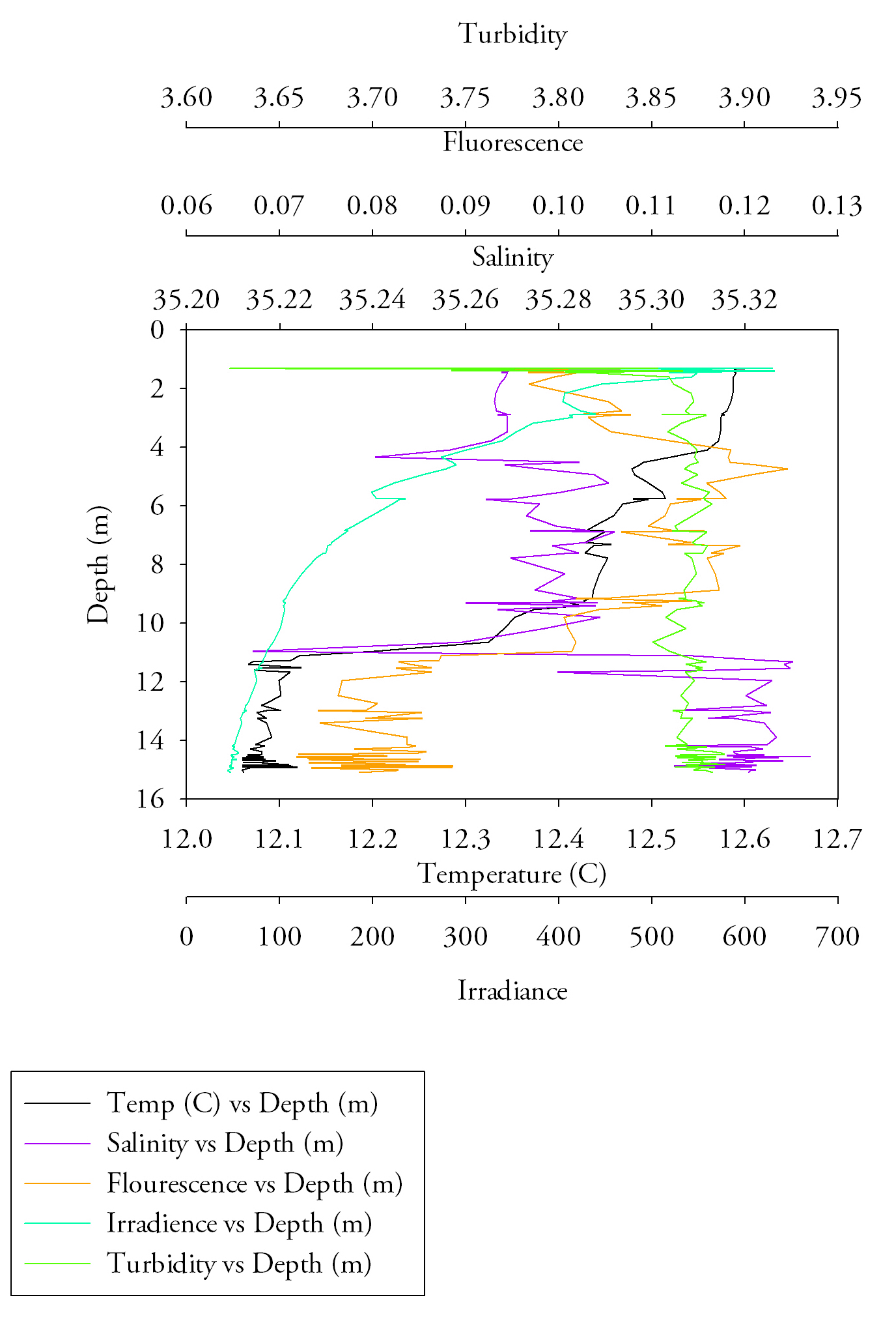
Fig.21. CTD data depth profile from station 5, click to enlarge |
Station 5 (Fig.21.) exhibits the same patterns in temperature, irradiance and fluorescence as stations 2,3 and 4 in that all changes that occur are very small thus demonstrating a highly mixed water column. In this data there does not appear to be any discernible thermocline, however there is a small halocline present at 7.34m from 35.26 to 35.28. below this small halocline fluorescence begins to decline to a minimum of 0.072. DiscussionAt station 2 it is clear that a greater temperature would extend down to greater depths during the summer months. They usually become thermally vertically stratified during these warmer months. The extent to which these waters become stratified in this way is due to the depth of the water and the tides, there type and there magnitude. The stratification parameter can be used to quantify the extent to which the waters are mixed (Pingree & Griffiths, 1978). Numerically this can represented: As the stratification parameter = Log (h/u3)
|
The main aim was to look at ‘how do vertical mixing processes in the waters off Falmouth affect, directly and indirectly, the structure and functional properties of plankton communities?’
The input of freshwater wind stress and rainfall can all affect the data collected in the offshore investigation. At station 4 the thermocline is at a greater depth this could have been forced downwards by greater wind stress over the surface and more mixing within the surface waters.
This vertical mixing is important when looking at the region of phytoplankton blooms. Other studies in the western English Channel have observed that phytoplankton respond to fluctuations in the physical and chemical properties of the surface layer of the ocean. Light and chlorophyll in the water column can give indication of the abundance of blooms and the location of them in the surface waters. Obviously the zooplankton will correlate to the phytoplankton. The distribution of dissolved oxygen is an indicator of the balance between autotrophy and heterotrophy.
In the summer months there is a nutrient depleted surface layer which is represented by the constant turbidity value as you travel down the water column shown on the graphs. It is often common to see some upwelling in these months to replace the nutrients that are being used. This is a typical process in coastal areas.
Station 5 was particularly interesting, with strong vertical shear down the water column with a strong west and east current flowing adjacent to each other. This was due to the station being near the headland, entrainment will cause mixing in the middle. However the water column will be stable, this is represented by the CTD graph in that the parameter lines are mainly vertical down the water column. Apart from temperature which has a slight thermocline around 8m but other than that decreases consistently with depth.
ADCP
As with the Estuarine physical analysis (above), an ADCP was used to measure current velocities, direction and acoustic backscatter within the water column, during the excursion, discrete profiles of the water column at each station where taken as well as transects between each station.
Transect 1 (Fig.25.1) - Station 1 - 2The maximum depth of the water column is between 20 -40m the faster moving waters are found at the edges of the transect and in the deeper waters in this instance. The higher velocities have an approximate value of 0.624m/s. The direction of flow is predominantly Northwards at the edge of the transect. Looking more towards the centre of the transect the flow direction is more toward the East. Backscatter increases as you move up the water column. It is approximately 68dB at 36m depth and towards the shallower depths the first 5m, the backscatter is between 90-101dB. Transect 2 (Fig.25.2) - Station 2 - 3The maximum depth is around 30m, with the higher velocities being in the first 20m, ranging from about 0.3-0.6m/s. It is clear looking at direction that there is shear in the water column, the flow is eastward in the bottom waters. It is predominately northward flowing, as you move up the water column it. There is a small proportion that is westward flowing in the mid-waters. This could cause shear in the water column. There is a relatively high amount of backscatter across this transect. It is virtually all 80dB with a single region falling below this. This region extends up near surface waters. On the contrary there are some areas of exceptionally high backscatter, these again are found in the surface 5m and have values up to 119dB. Transect 3 (Fig.25.3) - Station 3 - 4Along this transect the depth ranges from 30m to 20m. The velocity magnitude is highest in the mid and surface waters. With values ranging from 0.3-0.6m/s. There are some slower velocities found at depth with values in the region of 0.029m/s. The direction of flow is mainly Eastwards through the entire transect and water column. The Backscatter is similar to other transects observed in that there is high backscatter at the surface waters with a value of 119dB. The majority of the water column has a backscatter value of 72 dB. |
1.Transect 1 (station 1 - 2) Fig.25. ADCP transects for the offshore transect, between stations. |
Transect 4 (Fig.25.4) - Station 4 - 5
The depth along this transect to which it was measured is at a constant 20m. There is a clear difference within the water column. There is a strong vertical shear found in the water column between two oppositely moving water masses. The water moving Eastwards on the left of the transect is moving faster with a velocity of 0.8m/s. Compared to the water body moving mainly in the West direction that moves slower with an average value of velocity at 0.2m/s. In terms of backscatter it is similar to other transects. There are patches of high backscatter on the surface with values reaching 120dB. The average backscatter across the entire water column is approximately 80dB. There are areas of low back scatter that extend upwards from the sea floor with figures around 54dB.
Richardson number analysis
Station 1 (Fig.26.)The Richardson number shows the water column is laminar at the surface and therefore is more stable. It also shows that turbulent flow is increasing as depth increases to 7.5m. This is likely to be attributed to wind stress at the surface. There is laminar flow between 7.5m and 17.5m, where a large thermocline occurs which contributes to more stable flow. Because of the fluctuations in temperature after the thermocline the water column becomes more unstable demonstrated by a re number less than 0.25. Due to no other influencing factors the Richardson number begins to increase after the thermocline, to a more stable flow. This shows that tidal affects are weak. |
Fig.26. depth profile of richardson numbers at station 2. click to enlarge |
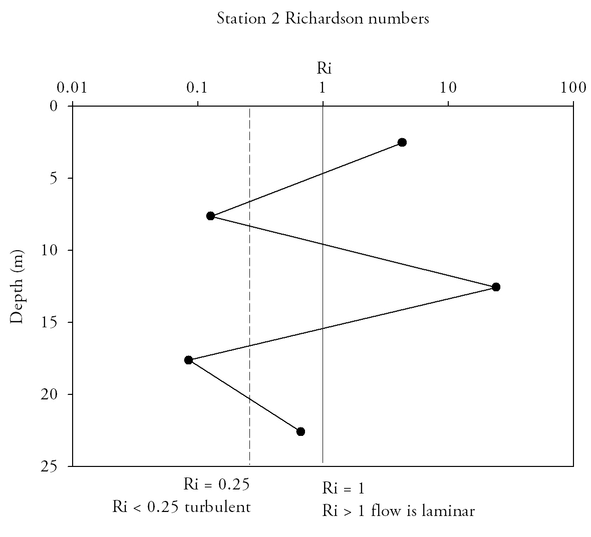
Fig.27. depth profile of Richardson numbers at statin 3. Click to enlarge. |
Station 3 (Fig.27.)Between 0 and 30 meters there is a gradual thermocline thus contributing to the progressive increasing stability with depth. An Ri number of 0.05 which is less than 0.25 gives a turbulent flow at the surface, this is induced by wind stress. The water column becomes laminar (Ri > 0.25) at a depth of 6.3m. This shows that the water column is very well stratified in two layers; a surface turbulent layer and a deeper laminar layer. |
Station 4 (Fig.28.)For this station taken just off the headland the surface Ri number is in the uncertainty zone, between 0.25 and 1, so could be considered to be turbulent or laminar. The surface this value is more likely to be turbulent due to strong winds over the surface at the time of measurement. The rest of the water column is laminar, due to a clear thermocline over 4-10m, showing that the column may be stratified. The headland will have high acceleration of flow around it which could be an influencing factor on the data. |
Fig.28. depth profile of Richardson numbers for station 4. Click to enlarge. |
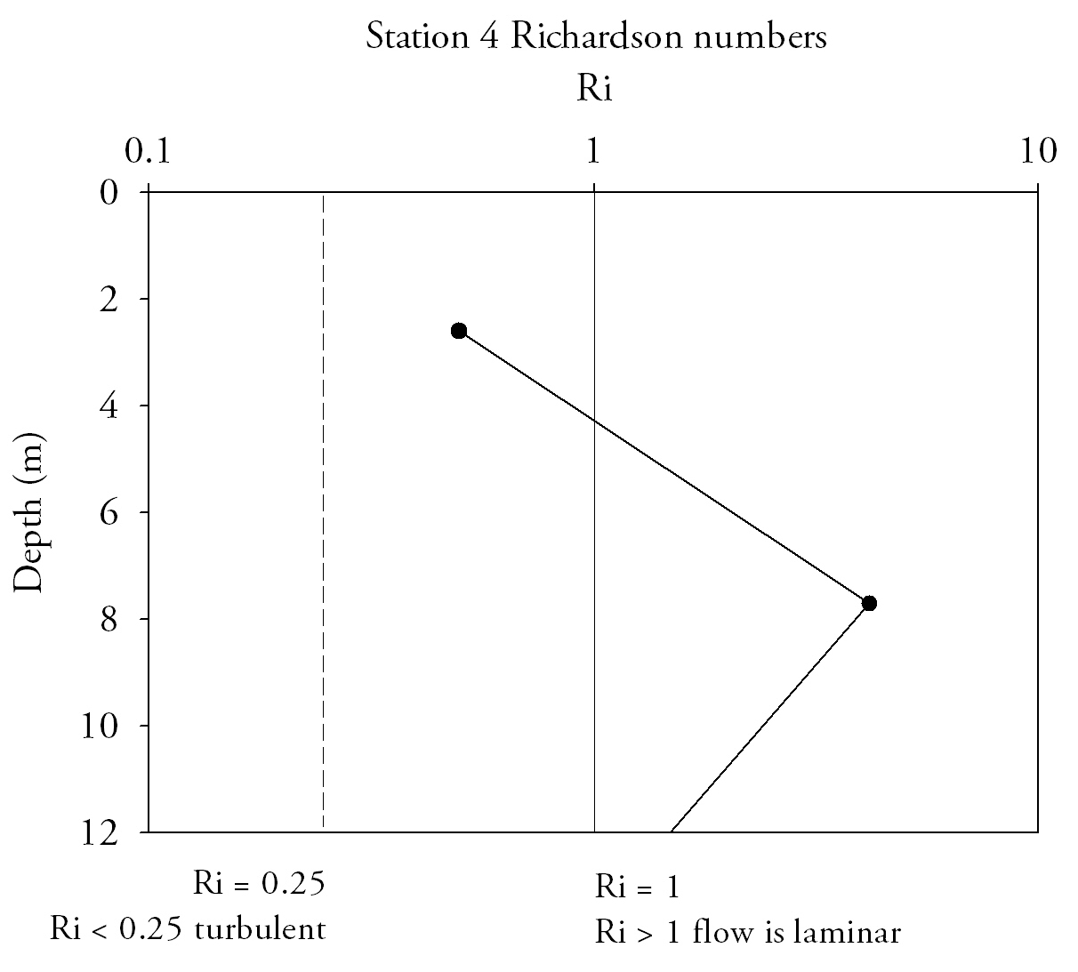
Fig.29. Depth profile of Richardson numbers for station 5. Click to enlarge. |
Station 5 (Fig.29.)The surface Ri number is 2.5m which is representative of turbulent flow. This again is due to wind stress on the surface and high velocities of flow. The flow becomes laminar and stays laminar between 5m and 20m, which are due to the gradual thermocline over this depth. The flow is turbulent below 20m, induced by high tidal velocities heading into the coast. This structure in the water column is indicative of a stratified flow, with two layers of turbulent mixing separated by a stable laminar layer. This station was just around from the headland so the stratified layers may be a result of the sheltered waters. |
Geophysical Habitat Mapping
The ROV (Remolty Operated Vehicle) used on the Xplorer is owned by the London Natural History Museum, costs about
£40, 000 and has a High Definition Camera setup that only exists on two ROVs in the world! Two operators were needed for the manipulation of the ROV, one to deploy it, and another one to manoeuver it. The submersible was connected to a console as well as a controller and a monitor. It has thrusters which are able to alter speed and direction through the controller. A copper cable transfers a video signal to the monitor the output from this was used as an extra tool for habitat mapping.
The side scan sonar was used in conjunction with a tow fish which was dropped and dragged at the back of the Xplorer. The acoustic pulse emitted from the transducer on the sidescan was reflected by the seabed features, the different seabed features printed on a thermal paper could then be distinguished.
The backscatter, once amplified, was transferred via a cable onto the recording unit onboard. Due to the difference in wavelength backscattered to the transducers. The side scan sonar was launched at 50° 12’ 00.7278N and 005° 02’ 15.7998W and was recovered at 50° 11’ 31.2144N and 005° 02’ 03.3372W. Only one transect could be done as a problem occurred with the sonar.
The drop down camera sits on a fish on which two torches are attached. The one used on the Xplorer was worth about £150. An operator on the deck was necessary to deploy the fish and readjust its position. A cable links the camera to a monitor, the video shown on the monitor allowed us to detect any change in habitat and the video was recorded on a CD for subsequent analysis. The drop down camera was used across the transect done for the sidescan sonar. It was launched at 05° 02’ 03.3372W and 50° 11’ 31.2144N and recovered at 05° 01’ 50.1430W and 50° 11’ 43.6680 N.
The results from the sidescan analysis and drop cam transect are displayed in this Poster designed for A2 print size.
Equipment
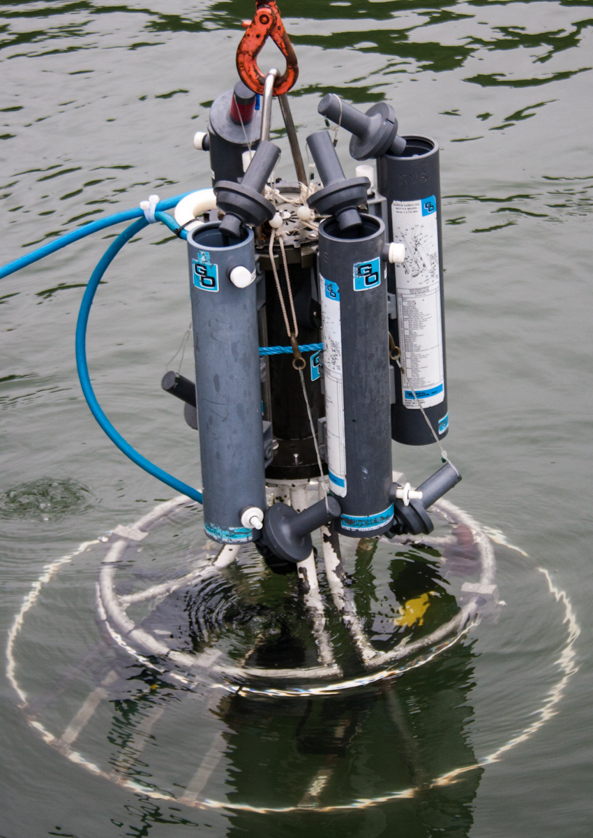
CTD (Conductivity, Temperature, Depth) rosette samplerCTDs are used on most research vessels to establish vertical profiles of salinity and temperature, and can include packages containing sensors such as chlorophyll fluorometer and transmissometers. These can be found on R.Vs Callista and Bill Conway and other sensors to measure dissolved 02, pH, light attenuation, sound velocity and more.
|
 |
 |
ADCPADCP are used on the back of research vessels, lowered into the water column, along with CTDs or attached to moorings. The ADCP mounted on a boat is used at depths greater than 1.5m. Flow velocity is recorded continuously along transects and the accuracy of the data transmitted to a computer (Herschy, 2009). How ADCPs work (National Oceanography Centre website) |
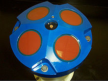
Secchi Disk
|
 |
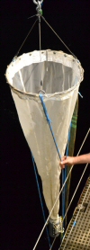 |
Plankton NetPlankton nets are cone shaped and made of a 200 micron mesh. The mouth of the cone has a diameter of 0.5m and the mesh will then filter the water flowing in the mouth. The part of the net with the smallest diameter is connected to a plastic bottle in which phytoplankton smaller than 200 microns are collected. The bottle has a cod end which allows plankton too large to go through the mesh to be restrained (Sigler and Sigler, 1990). Some plankton nets, such as the one deployed on R.V. Callista, are closing plankton nets, meaning that they can target a specific depth interval in the water column, close up, and be recalled to the surface without collecting any more plankton. |
Sidescan SonarSidescan sonar are used in conjunction with a tow fish and launched from the back of a research vessel and uses acoustic waves from 1kHz up to 100 MHz to determine the topography of the seabed (Blondel, 2009). An acoustic pulse is emitted from the transducer and reaches the seabed where it is backscattered by seafloor features to the transducer, amplified and transferred via a cable onto a recording unit onboard (Kenny et al., 2003). The scale of the seabed features depends on the different acoustic pressures that are backscattered to the hydrophone on the sonar. The position of each seabed feature is recorded by the recording unit on the vessel pixel by pixel in order to be able to analyse features ranging from tens of centimeters to a hundred meters. The sidescan output is then printed either on thermal paper or electro sensitive paper. |
 |
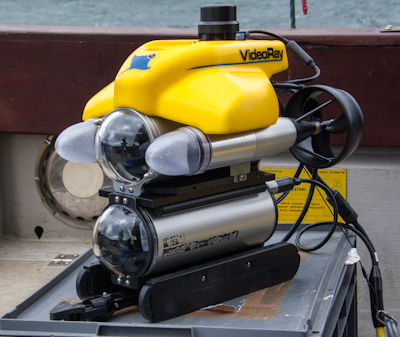 |
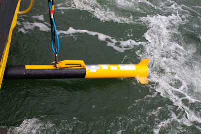
Remotely Operated Vehicles (ROVs)Remotely Operated Vehicles can be manned or unmanned and have various purposes ranging from cleaning of boats’ hull to construction and maintenance of drilling platforms. A drop camera was also utilised, hung on a cable below the ship, the camera was drifted just above the sediment surface, providing footage of the seabed.
|
YSI probeThe 6600 V2 YSI probe is a multi-probe measures conductivity (salinity), temperature, chlorophyll a, dissolved oxygen and pH. It can be deployed into the water by hand while values are displayed by a computer on deck. Light MeterThe light meter consists of two sensors; the air sensor and the water sensor. When the two sensors are calibarated; the difference between them indicates light attenuation through the water column, percentage light levels certain depths can then be calculated.
|
R.V. CallistaRV Callista is a purpose built twin hulled research vessel commissioned By the University of Southampton and built in Finland. She was built to provide practical experience for students that are studying various elements of Oceanography at the University of Southampton. She is equipped with some of the latest technology for monitoring coastal and estuarine environments in situ, such as an on-board ADCP unit. She has purpose built wet and dry labs, a galley area and is able to sleep up to 4 crew members. |
 |
 |
R.V ConwayRV Conway is a University of Southampton owned multi-use research vessel. It can be outfitted with a variety of equipment to carry out specific scientific operations. It has an open rear deck area with a covered wheelhouse in which scientific computer based programmes can be run from onboard computers. Its primary use is for coastal and inshore work and is equipped with a 750kg A-frame with a trawl cable setup which extends up to 70 metres. |
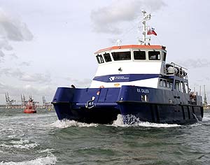
RV XplorerXplorer is a vessel contracted to us to assist us in our studies of the Falmouth estuary and the surrounding area. She Is a purpose built MCA category 2 survey vessel built in 2002 by Gemini Workboats in Plymouth. Her primary role is as a survey and diving support ship, which makes her ideal for carrying out our side scan sonar work in the Falmouth Estuary. It has a large rear deck area with a 1 tonne capacity crane with facilities for dry labs in the wheelhouse. |
 |
References
Birt, J., 2004, A review of nutrient studies and factors influencing nutrients in the coastal waters of south west England, [Online]. Available: www.cornwall.ac.uk/cc/index.php?dlrid=218 [accessed 2012, July 4th]
Blondel, P., 2009, The Handbook of Sidescan Sonar, Praxis Publishing, Chichester, United Kingdom.
Bryan, G.W. and Gibbs, P.E., 1983, Heavy metals in the Fal estuary, Cornwall: A study of long term contamination by mining waste and its effects on estuarine organisms. Occasional Publications. Marine Biological Association of the United Kingdom, 2, 112.
Christ, R.D., 2007, The ROV manual user guide for observation class, remotely operated vehicles, Elsevier, Oxford.
Cloern, J.E., 1987, ‘Turbidity as a control on phytoplankton biomass and productivity in estuaries Continental Shelf Research, 7, 1367–1381.
Eloire, D., Somerfield, P.J., Conway, D.V.P, Halsband-Lenk, C., Harris, R. 2010, ‘Temporal variability and community composition of zooplankton at station L4 in the Western Channel: 20 years of sampling’, Journal of Phytoplankton Research, 32, 657-672.
Grasshoff, K., Ehrhardt, M., Kremling K., 1999, Methods of seawater analysis, Verlag Wiley-VCH, Weinheim.
Hansen, D.V. and Rattray, M., 1966, ‘New dimensions in estuary classification’, Limnology and Oceanography, 11, 319–326.
Herschy, R.W., 2009, Stream flow measurement, third edition, Taylor and Francis, Oxon.
Holligan, P.M. & Harbour, D.S., 1977, The vertical distribution and succession of phytoplankton in the western English Channel in 1975 and 1976. Journal of Marine Biological Association of the United Kingdom , 57, 1075-1093.
Jarvie, H.P., Haygarth, P.M., Neal, C., Butler, P., Smith, B., Naden, P.S., Joynes, A., Neal, M., Wickham, H., Armstrong, L., Harman, S. and Palmer-Felgate, E.J., 2008, ‘Stream water chemistry and quality along an upland-lowland rural land-use continuum, south west England’, Journal of Hydrology, 350, 215-231.
Kenny, A.J., Cato, I., Desprez, M., Fader, G., Schuttenhelm, R.T.E., Side, J. 2003, ‘An overview of seabed-mapping technologies in the context of marine habitat classification’, ICES Journal of Marine Sciences, 60, 411-412.
Kimmerer, W.J., Burau, J.R. & Bennett. Tidally orientated vertical migration and position matinence of zooplankton in a temperate estuary. Limnol Oceanogr, 43, 7, 1697-1709.
Lalli, C.M., Parsons, T.R., 1997, Biological Oceanography, An Introduction, second edition, Elsevier Butterworth-Heinmann, Burlington.
Langston, W.J., Chesman, B.S., Burt, G.R., Hawkins, S.J., Readman, J. and Worsfold, P., 2003, ‘Site characterisation of the south west European marine sites: Fal and Helford cSAC’, Marine Biological Association of the United Kingdom Occasional Publication, 8.
Miller, C., 2004, Biological Oceanography. Blackwell Science. Malden.
Monbet, Y., 1992, ‘Control of phytoplankton biomass in estuaries: A comparative analysis of microtidal and macrotidal estuaries’, Estuaries, 15, 563-571.
Parsons et al., 1984, A Manual of Chemical and Biological Methods for Seawater Analysis. Pergamon Press. Pons Point, N.S.W. Australia.
Pelletier, P.M., 1988, Uncertainties in the single determination of river discharge—A literature review: Canadian Journal of Civil Engineering, 15, 5, 834–850.
Pingree R.D., Maddock L. & Butler E.I., 1977, The influence of biological activity and physical stability in determining the chemical distributions of inorganic phosphate, silicate and nitrate. Journal of the Marine Biological Association of the United Kingdom, 57, 1065-1073.
Pingree, R.D. and Griffiths, D.K., 1978, Tidal fronts on shelf seas around the British Isles. J. Geophys. Res. 83 (C9), 4615-4622.
Preseindorfer, R.W., 1986, ‘Secchi Disk science: visual optics of natural waters’, Liminology and oceanography, 31, 909.
Queiroga, H., Costlow, J.D. & Moreira, M.H., 1997, Vertical migration of the crab Carcinus maenas first zoea in an estuary: implications for tidal stream transport. Marine Ecology Progress Series, 149, 121-132.
Royal Commission on Environmental pollution, 2004, Turning the tide, Addressing the impact of Fisheries on the Marine Environment,Crown, Norwich.
Ryabov, A.B., Rudolf, L. & Blasius, B., 2010, Vertical distribution and composition of phytoplankton under the influence of an upper mixed layer. Journal of Theoretical Biology, 263, 120-133.
Seuront, L. and Schmitt, F.G., 2005, ‘Multiscaling statistical procedures for the exploration of biophysical couplings in intermittent turbulence’, Deep-Sea Research II, 52, 1325-1343.
Sigler, W.F. and Sigler, J.W., 1990, Recreational Fosheries, Management, Theory and Aplications, University of Nevada Press, Nevada, United States.
Vidussi, F., Claustre, H., Manca, B., Luchetta, A. and Marty, J., 2001, Phytoplankton pigment distribution in relation to upper thermocline circulation in the eastern Mediterranean Sea during winter. Journal of Geophysical Research 106(C9).
Widdicombe, C.E., Eloire, D., Harbour, D., Harris, R.P. & Somerfield, P.J., 2010, Long-term phytoplankton community dynamics in the Western English Channel. Journal of Plankton Research, 32, 5, 643-655.
The views and opinions expressed in this website do not reflect those of the
University of Southampton or the National Oceanography Centre.
Published June 2012. All rights reserved.