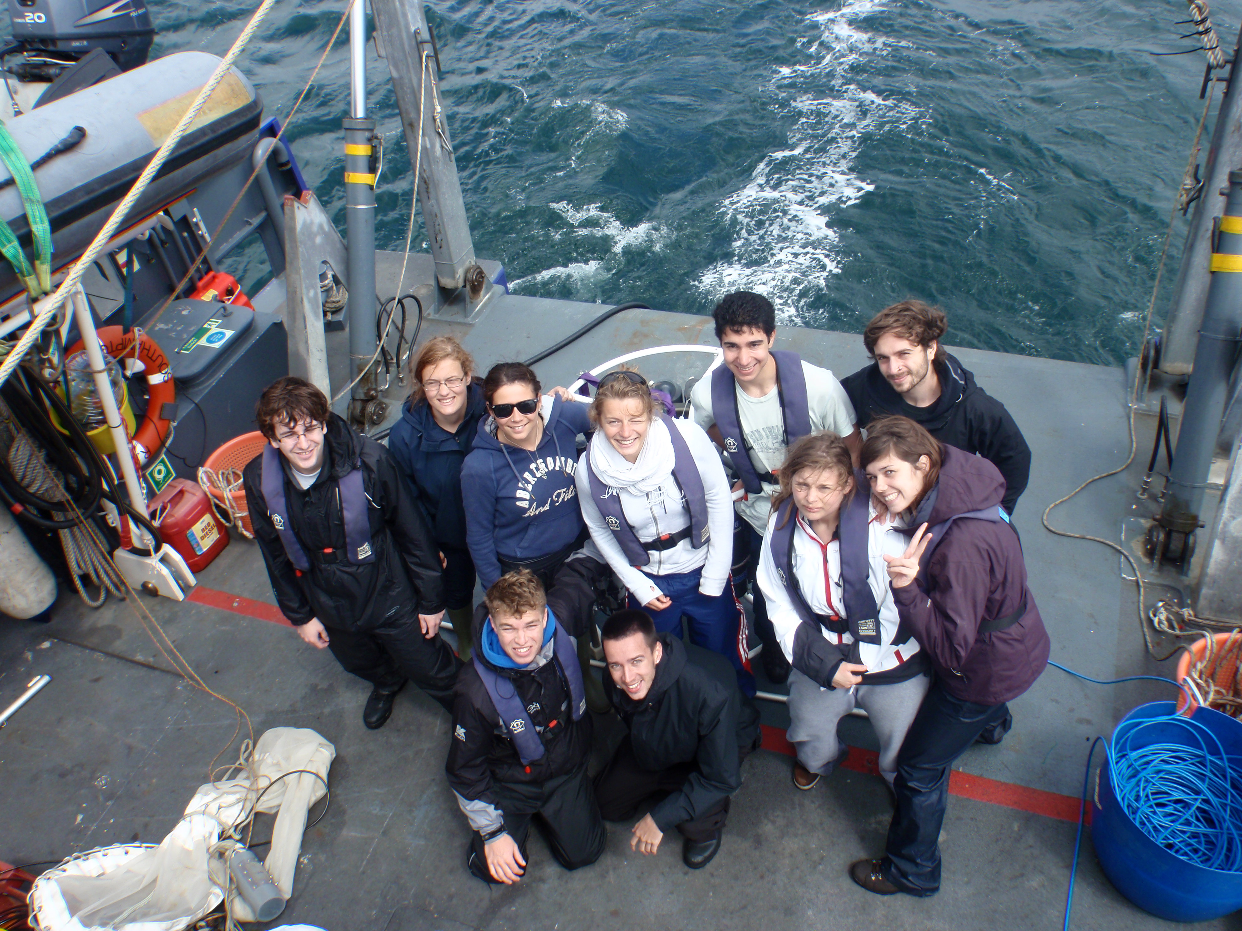
Falmouth Field Course - Group 4
|
Tom Ivey |
Lucy Dickinson |
|
Jeremy Mirza |
Hannah Brown |
|
Amber Cobley |
Josh Fernandez |
|
Anthony Zardis |
Charlotte Blick |
|
Tom Le Tissier |
Kat Barnes |
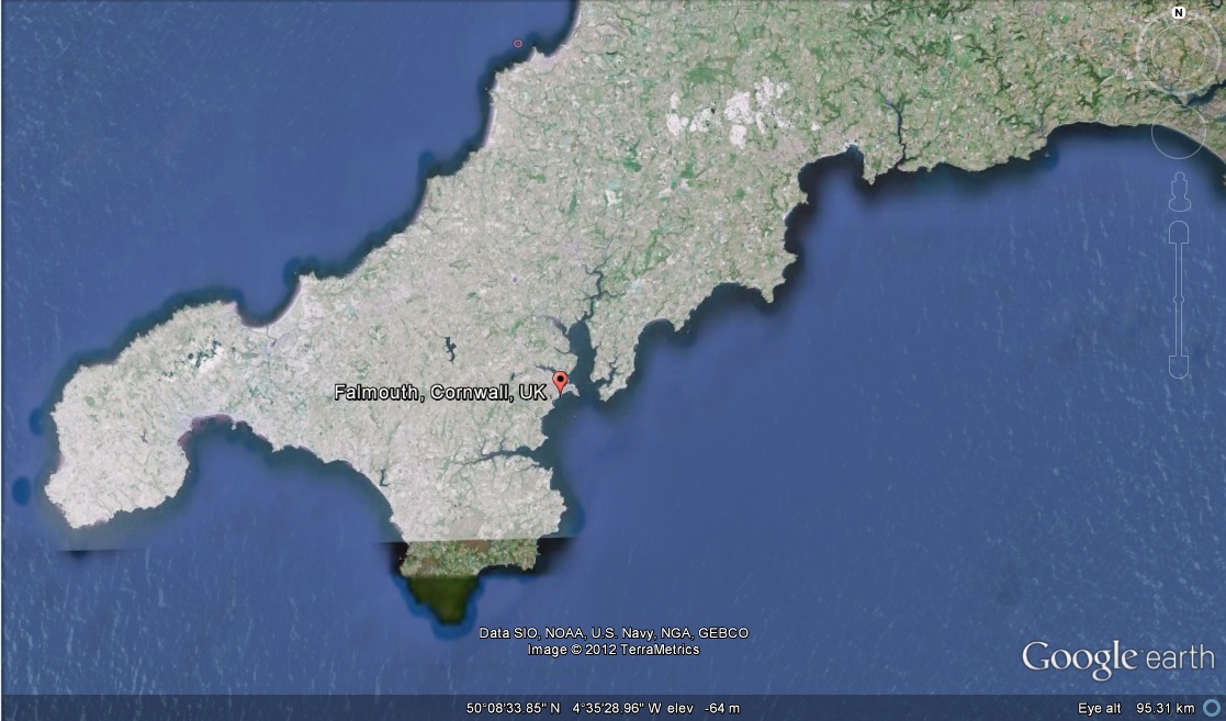
Fal Estuary is a ria, flooded river valley, formed by sea level rise. The Fal estuary and Helford River area is a Special Area of Conservation (SAC) which is selected under the “The Habitats Directive” legislation to highlight the need to maintain biodiversity throughout the European Community, with special emphasis on rare or threatened habitats or species.
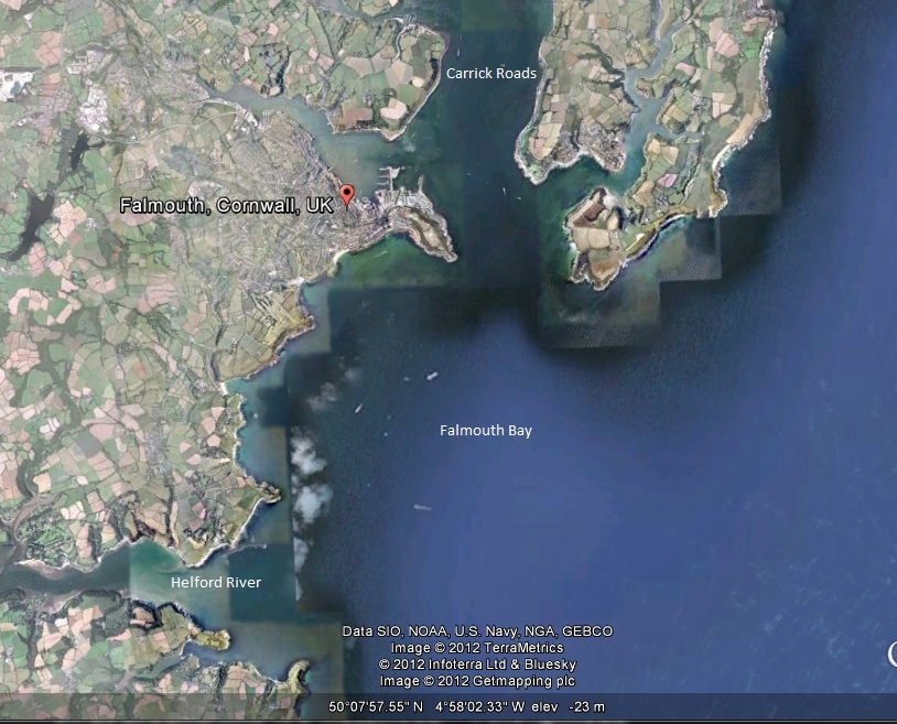
Anthropogenic pollution has entered the Fal Estuary on several different occasions and continues in small volumes. The most significant was the release of mining waste containing high concentrations of heavy metals. 50 million litres of acidic, metal laden water flowed into the estuary in 1992 and 13,600 litres of waste oil being dumped in Falmouth dock in 2009. This pollution is most noticeable by high concentrations found in the sediments. It is less obvious in the water itself.
In this investigation we aim to survey the Fal estuary and the surrounding waters in order to make a estimation of potential impacts of dredging using habitat mapping. We aim to make a thorough survey of the water column in several locations to analyse temperature, salinity, biological activity, chemical and physical parameter, nutrients, mixing and water column stability.
|
Date (June/July 2012) |
Activity |
|
Mon 25th June |
Arrive |
|
Tue 26th June |
Geo am Web pm |
|
Wed 27th June |
Geolab am Estuary TS |
|
Thurs 28th June |
Estuary lab |
|
Fri 29th June |
Offshore |
|
Sat 30th June |
Offshore lab |
|
Sun 1st July |
- |
|
Mon 2nd July |
Data |
|
Tues 3rd July |
Pont pm |
|
Wed 4th July |
Data |
|
Thurs 5th July |
Data |
|
Fri 6th July |
Data |
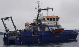
RV Callista is a twin-hulled catamaran and has a MCA Workboat Certification category 2 which is licensed to 60 miles offshore. It is an ocean going research vessel, purpose built and designed for scientific surveys, equipped with wet and dry labs and carries CTD, hull mounted 600Khz ADCP, plankton net, secchi disk and GPS.
It has a 20m (draught 1.8m), a top speed of 15kts with a standard cruising speed 10kts and a range of 400 nautical miles. We took these limitations into account when planning survey work as we were limited by time and distance. Stern mounted “A” frame with a lifting limit of 4 tonnes, hydraulic crane, stern winch and 150m cable allowing it to be used for a variety of equipment.
Large back deck, wet lab and dry labs enable preparation and analysis of samples and equipment. Data can be recorded, analysed and stored whilst at sea, reduced errors in transportation back to land based lab analysis.
We deployed the CTD at each station to give a vertical profile of the water column at that site. We used Niskin bottles fired at specified depths to take water samples particularly at depths where there was a chlorophyll maximum indicated on the fluorometer.
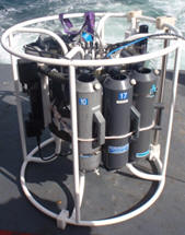
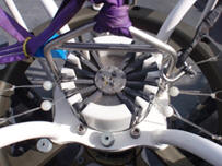
Fig 3
Callista bottle trigger system - each bottle is loaded to a hook which is assigned a firing number. Electronic pulses are sent to the bottle rosette via a power cable to release the hook and close the bottle when the required depth is reached.
Samples must be taken on the upcast so the high pressures at depth don't damage the bottles. The firing is controlled by computer program using a simple "fire bottle" button. A light would indicate which bottle has been fired.
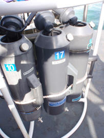
Fig 4
The area of the net entrance multiplied by the depth over which it was deployed gives the volume of water the net has passed through. One issue we found with this was the strong wind and surface current caused the net to move horizontally meaning the depth sensor readings and the volume of water through the net were inaccurate.
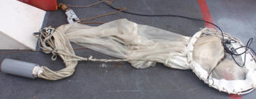
Fig 5
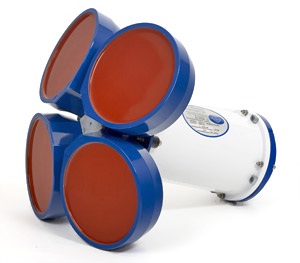
The ADCP emits a sound pulse from the transducer into the water column. The transducer will have 3 or 4 heads (sources of sound pulses) which allows the time difference in the return of the separate pulses to be measured. The Doppler shift (stretching or compressing of sound waves due to water movement away or towards the source of sound) allows a profile of the water movement to be formed.
Higher frequency provides greater accuracy but a smaller range, due to higher frequency sound being attenuated faster than lower frequency sound.
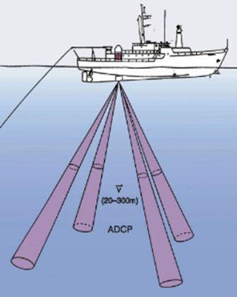 Fig 6
Fig 6
Coastal research vessel designed for scientific surveys, lab and carries CTD, ADCP, plankton net, secchi disk and GPS. 12m long designed specifically for coastal research. Certified to 60miles offshore with a standard cruising speed of 9kts and top speed of 10kts, with a range of 150 nautical miles. Stern 750kg “A” frame and 70m trawl winch. Carries less equipment so can be outfitted for the specific role it will be undertaking.
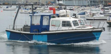
Fig 7
Fig
8
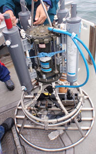 Fig 9
Fig 9
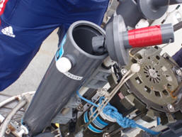
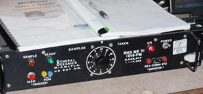
Fig 10
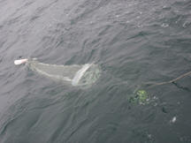
Fig 11
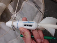
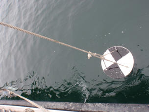 Fig 12
License for 60 miles offshore. Dimensions: 12m x 5.2m x 1.2m. 18kts cruise speeds with 25kts top speed. Extended wheelhouse fitted out for survey and dive support duties.Heila deck crane with winch. Hydraulic winch with 1 tonne lifting capacity. Survey equipment mounting brackets. Spacious clear working deck, stern door access, for divers & equipment.
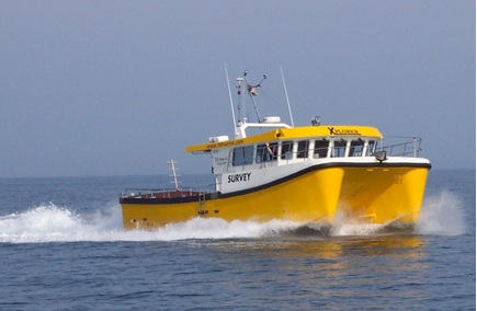
Fig 13
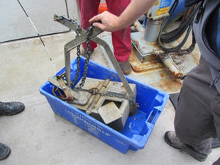 Fig 14
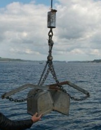
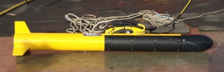
Fig 15
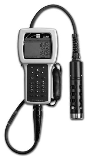
YSI Probe - Measures dissolved oxygen, pH, conductivity, temperature and Redox potential with depth.
 fig
16
fig
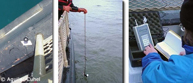
16Light meter - Comprises of two light sensors, one stays at surface, and one is lowered into the water. This corrects for varying incoming light levels caused by varying cloud cover.
 fig
17
fig
17Current Meter - Device used to measure speed and direction that the water is flowing at given depths when lowered into the water column.
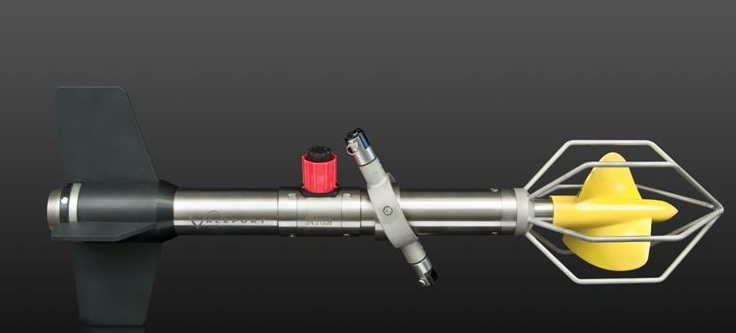 fig 18
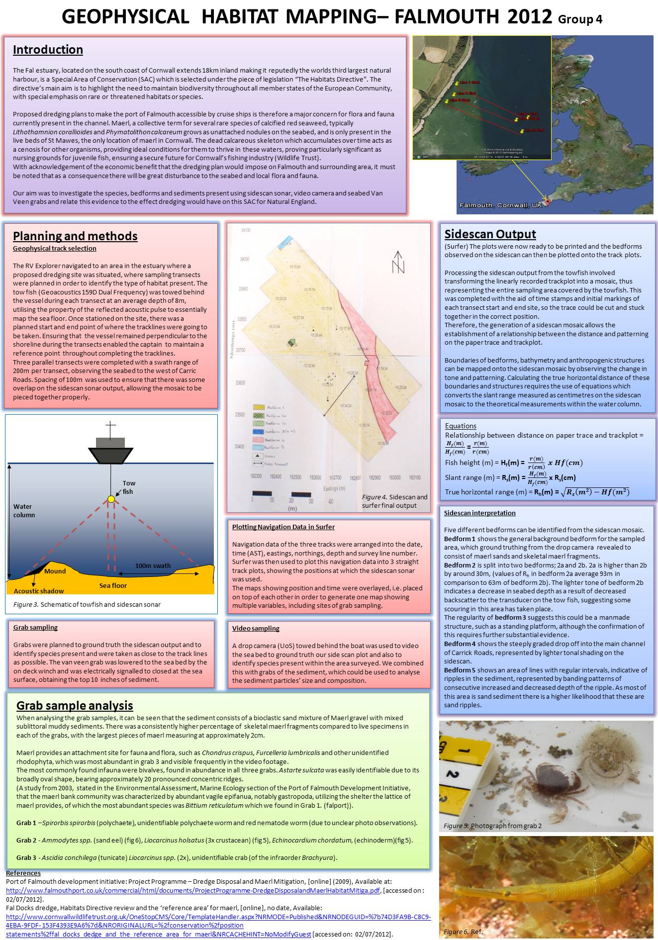
The main objectives of geophysical boat practical was to identify different habitat areas present and the species found over the survey area.
Key points to investigate
- potential effects of dredging channel on maerl beds.
- species present
- water flow direction and speeds dependant on tidal currents
- where will dredged sediment settle?
Maerl is a collective term for several species of calcified red seaweed, typically Lithothamnion corallioides and Phymatolithon calcareum and grows as unattached nodules on the seabed, who’s dead calcareous skeleton accumulates over long periods to form deep deposits, and important habitat.
The structure forms a latticework of “nooks and crannies”, providing a vital nursery ground for many commercial juvenile fish species, ensuring long-term future for Cornwall’s fishing industry (wildlife trust).
Maerl beds typically develop where there is some tidal flow but also in more open areas where sufficient wave action removes fine sediments but does not break the brittle structure. Tyler and Hiscock (2005) state that maerl is “highly intolerant” of “substratum loss” “smothering” “changes in suspended sediment” and “abrasions and physical disturbance” (Spencer-Hall, 2010).
“At present, the waters there are about 5m deep at low tide. We want to dredge to make a channel that is 8.5m deep. That would allow large cruise ships to moor at our docks. It would be good for business in Cornwall.” Falmouth Harbour Master. (Mckie,R. 2012)
Although economic benefits must be considered, when added together, an estimated 10,000m 3 of mud, sand and maerl per week will be excavated over 26 weeks. Cornwall Wildlife Trust are strongly against this development.
George Osborne has urged the project's approval saying "gold-plating of EU rules on habitats" was placing ridiculous costs on British business. He set up a government review of how EU directives on habitats and birds are being applied in England.
On top of this, the long accumulation period it takes for the dead calcareous skelton of the maerl to build up the habitat present means that the effects would be classed as a “major adverse impact”.
An independent report has stated that the use of a backhoe dredger should reduce the smothering of maerl to ~20m around the channel in comparison to suction dredging, however, this is still an action of major adverse effect possibly being given the go-ahead in an SAC.
It also raises the possible solution proposed initially by the developers of the mitigation and redistribution of the dredged maerl to a depth of 1m, however, the statement that this would reduce the impact to a “minor adverse residual impact” is subjective (Spencer-Hall,J. 2010).
The recovery rate of the habitat itself is relatively under studied. The Environmental Impact Assesment after dredging was prohibited in 2007, showed a much higher total number of individuals were recorded, with the average per core increasing from 90 to 265.
In terms of biodiversity, likely due to the intermediate disturbance hypothesis, infaunal communities in previous dredging extraction areas were found to be statistically significantly more diverse when measured as a Shannon-Weiner diversity index than site of little or no extraction (http://www.falmouthport.co.uk/commercial/html
/documents/SectionMarineandCoastalEcology.pdf) which could potentially be used as a counter-argument in this debate.
Once stationed on the site, there was a planned start and end point of where the tracklines were going to be taken. Ensuring that the vessel remained perpendicular to the shoreline during the transects enabled the captain to maintain a reference point throughout completing the tracklines.
Three parallel transects were completed with a swath range of 200m per transect, observing the seabed to the west of Carric Roads. Spacing of 100m was used to ensure that there was some overlap on the sidescan sonar output, allowing the mosaic to be pieced together properly.
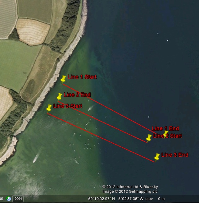 Fig 19
Line 1 was taken from 09:14:44 UTC to 09:20:48 UTC, with a start point of longitude 005o 02’53.7491 N, latitude 050o 09’57.2334 W. The end point was longitude 005o 02’20.8860 N, latitude 050o 09’43.355 W.
Line 2 was taken from 09:23:14 UTC to 09:28:40 UTC, with a start point of longitude 005o 02’26.6322 N, latitude 050o 09’42.4232 W and an end point of longitude 005o 02’55.6142 N and latitude 050o 09’53.43 W.
Line 3 was taken from 09:30:32 UTC to 09:36:16 UTC, with a start point of longitude 005o 02’59.456 N and latitude 050o 09’51.22 W, with an end point of longitude 005o 02’24.4466 N and latitude 050o 09’38.55 W.
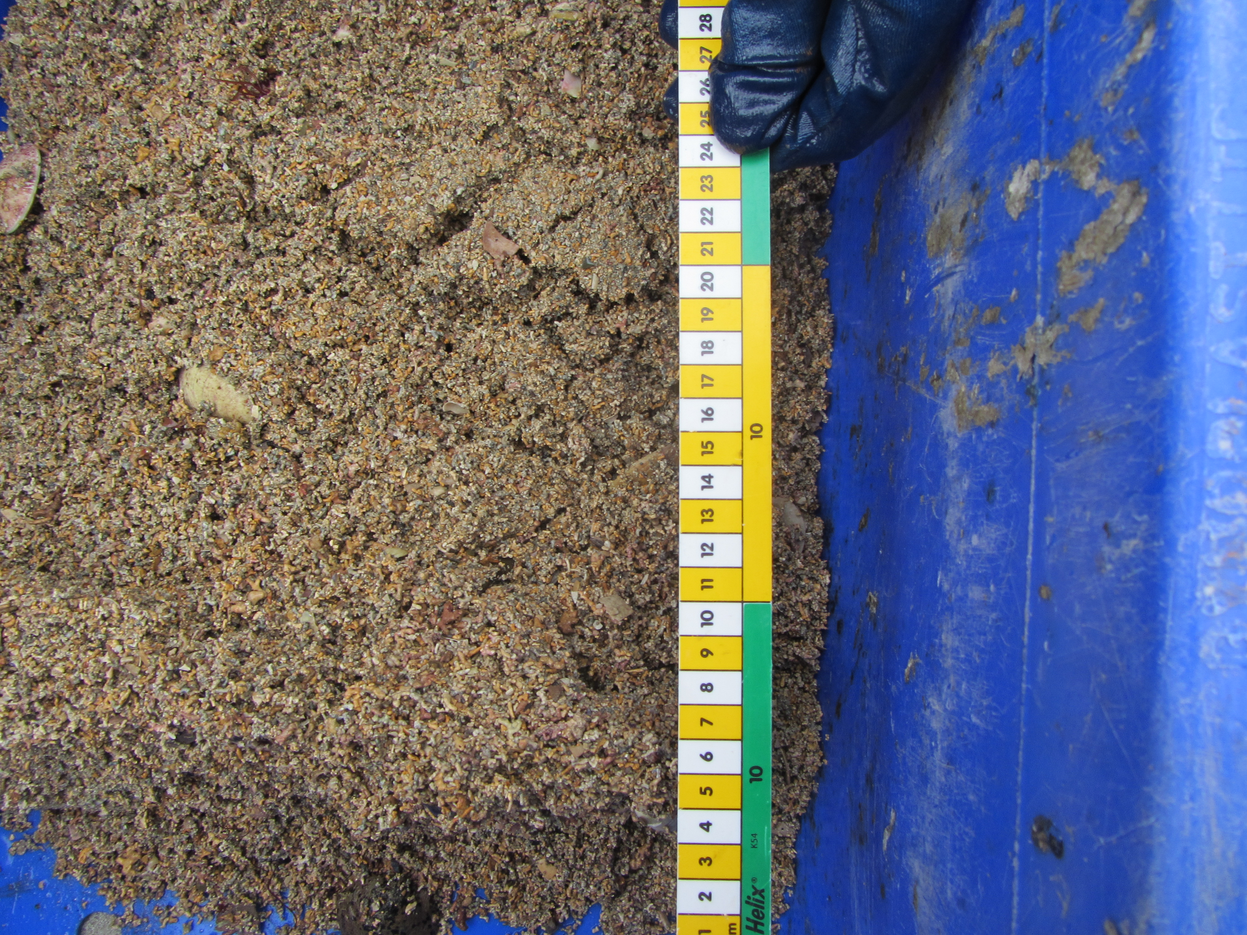
Grab 1 was taken at 10:00:08 UTC at longitude 005o 02’44.4576 N and latitude 050o 09’49.4616 W, with the seabed at 10m depth.
 fig
20
fig
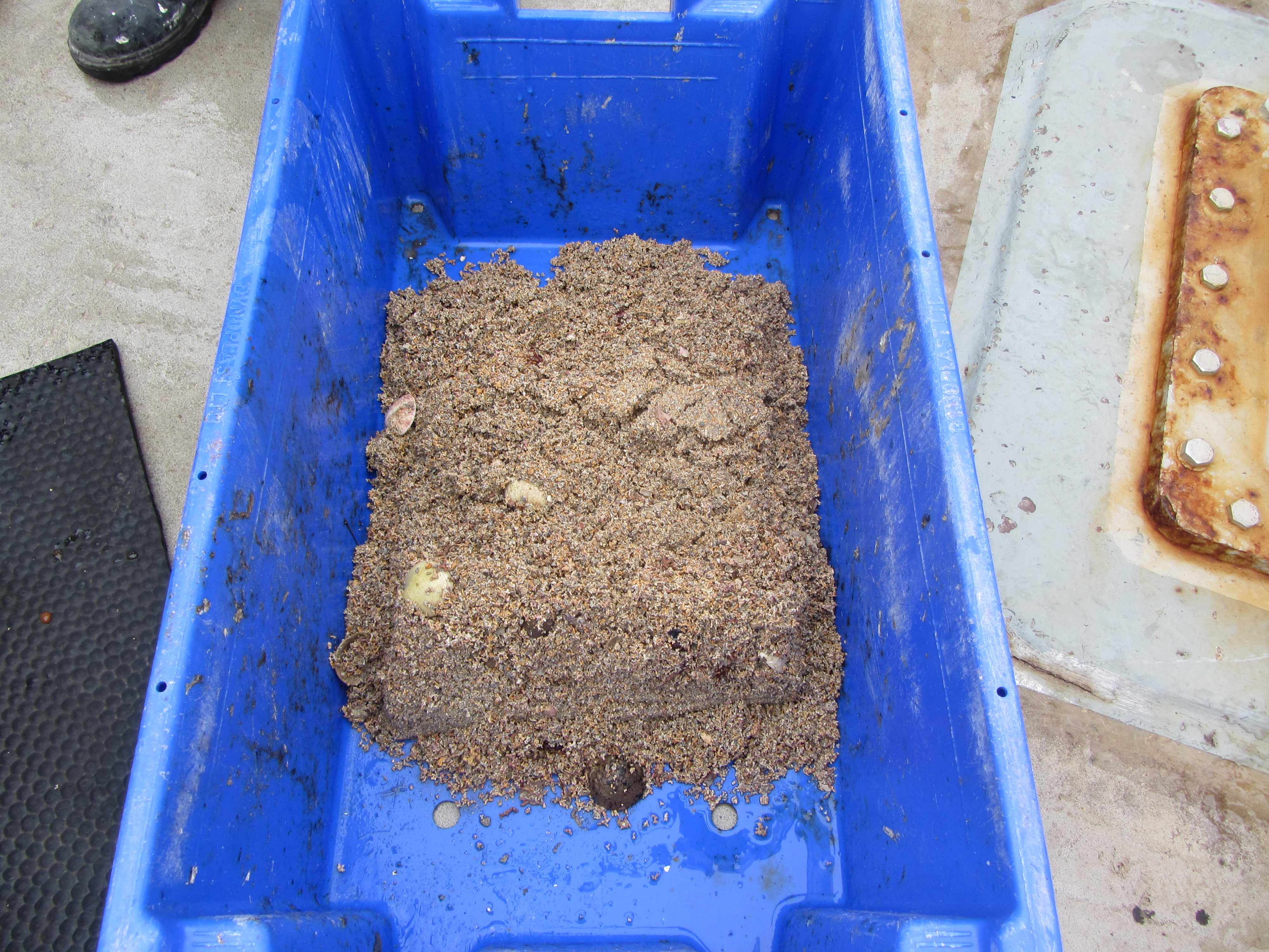
20Grab 2 was taken at 10:44:15 UTC at longitude 005o 02’38.3304 N and latitude 050o 09’56.5728 W, with the seabed at 9.3m.
 fig
21
fig
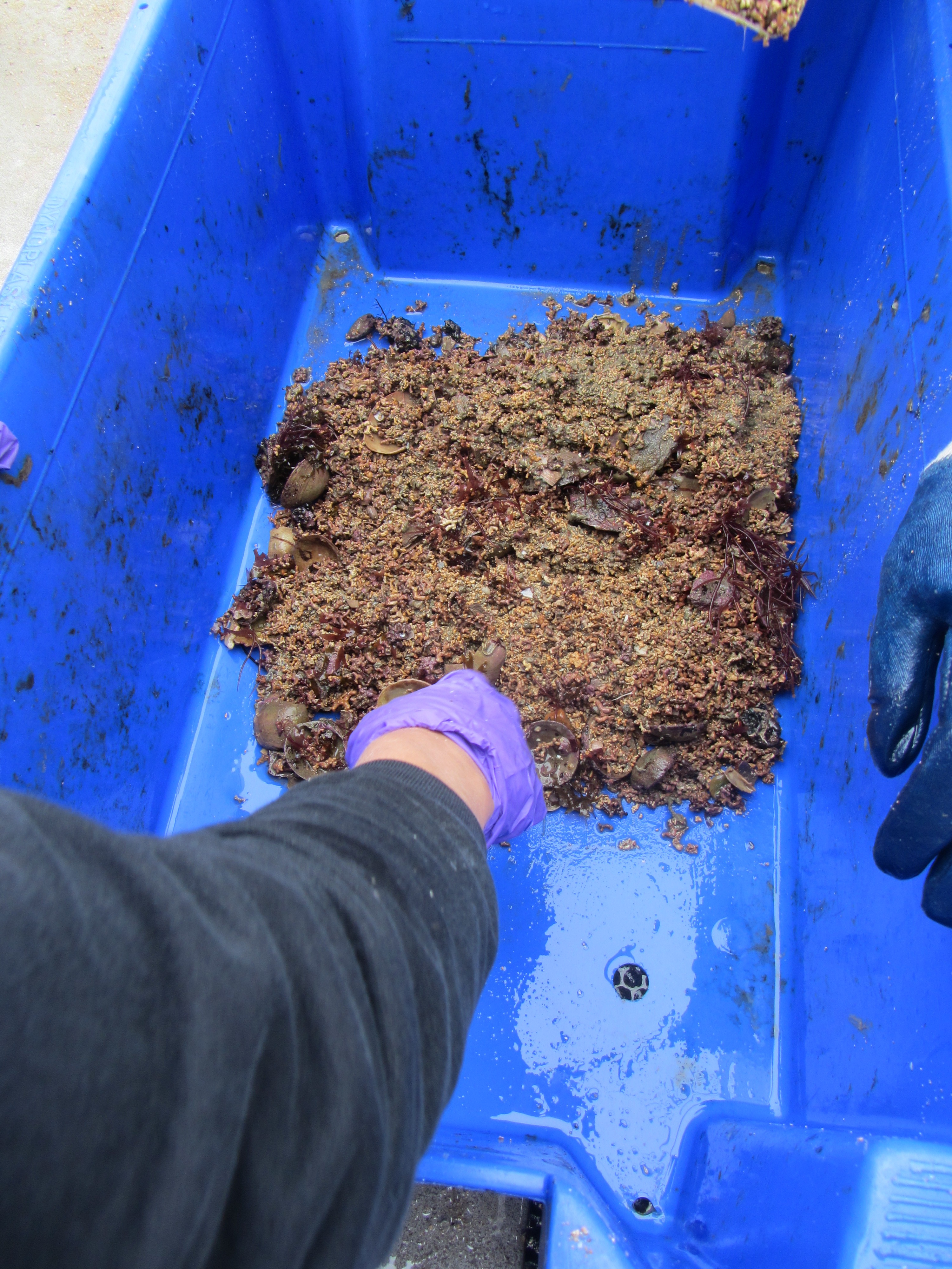
21Grab 3 was taken at 11:16:33 UTC at longitude 005o 02’40.0812 N and latitude 050o 09’43.0806 W, with the seabed at 10m.
 fig
22
fig
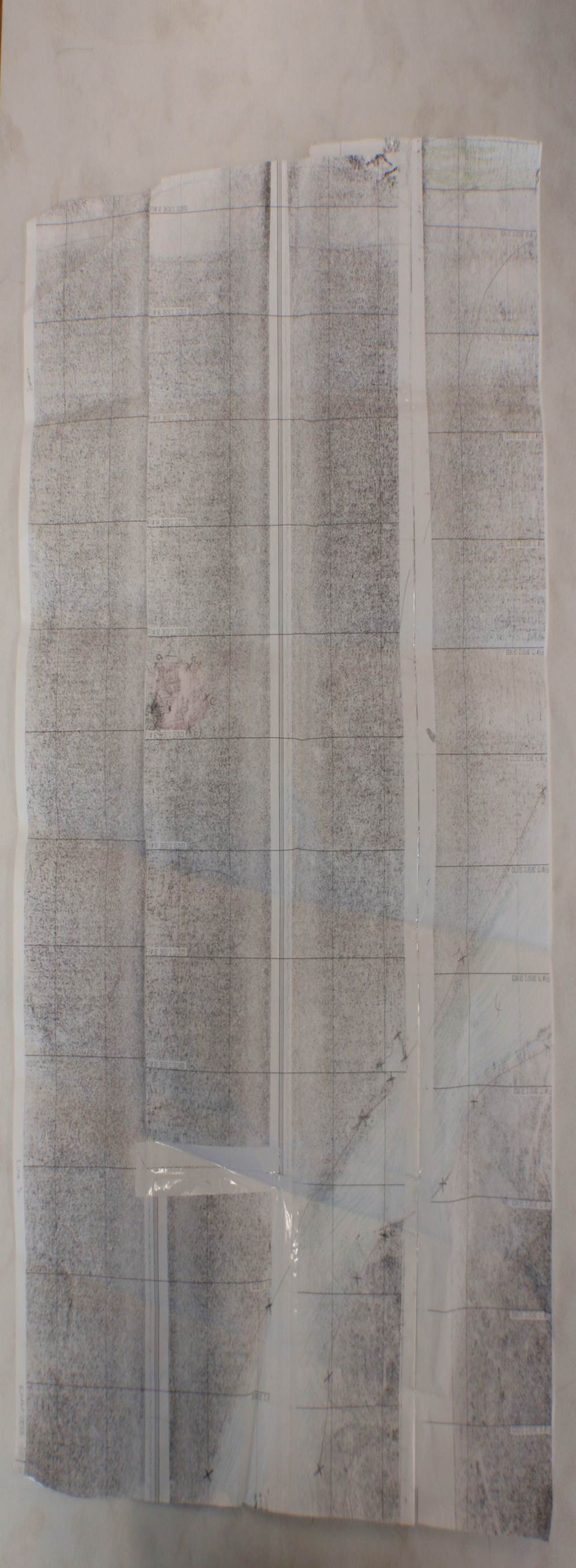
22Click link below to open Geophysics Poster
Click thumbnail below to view poster.
 Fig
23
Fig
23
Print out of the 3 track lines overapped and pasted together to form a mosaic, with annotations of features and bedforms by observing changes in patterning and tone.
 Fig
24
Fig
24
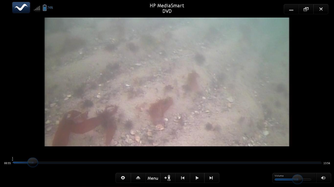
Still 1:
11:51:04.136,182731.72,33820.95,0.00,0.00,0.00,321.5,-146.10,
Ripples visible, shells/debris collected in trough of ripples.
Variety of green and red seaweed visible.
 FIg
25
FIg
25
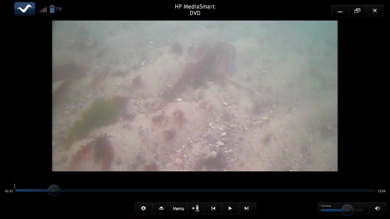
Still 2:
11:51:34.137,182732.35,33826.77,0.00,0.00,0.00,318.7,-151.27,
Ripples visible, shells/debris collected in trough of ripples.
Variety of green and red seaweed visible.
 Fg
26
Fg
26Still 3: 11:52:34.136,182733.68,33835.68,0.00,0.00,0.00,314.8,-159.39,
Shows shoal of fish
 Fig 27
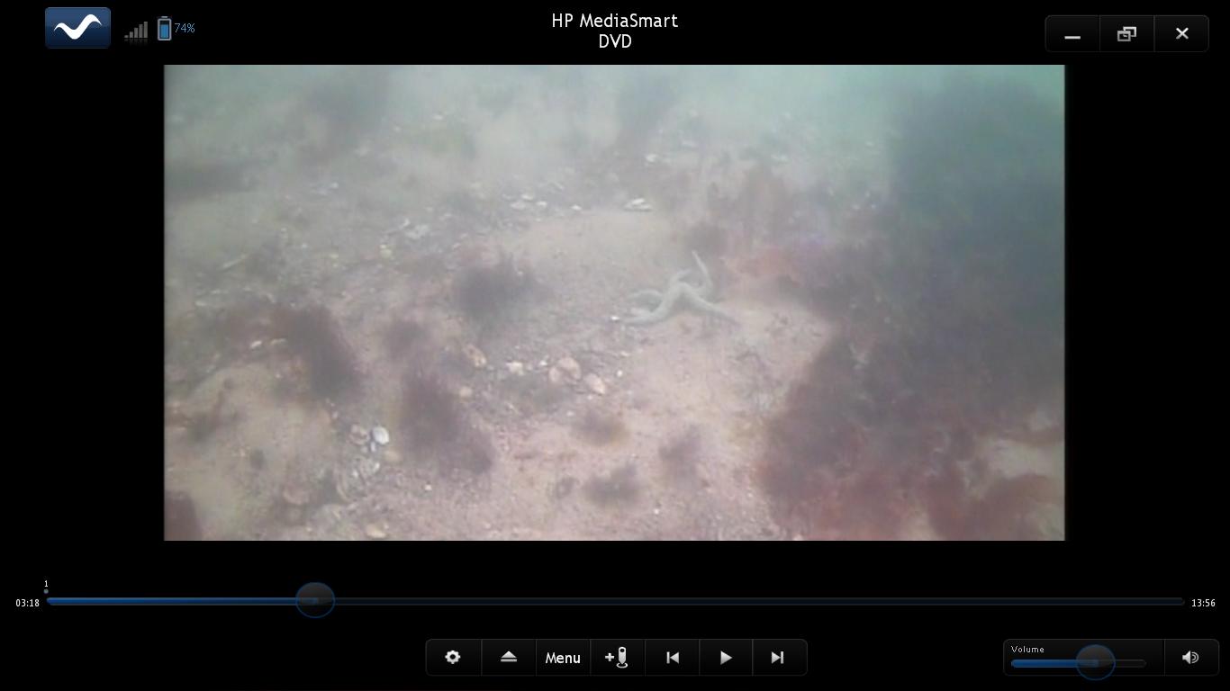
Still 4: 11:53:14.136,182733.84,33841.21,0.00,0.00,0.00,311.8,-164.05,
Echinoderm unidentifiable beyond class Asteroidea
 Fig
28
Fig
28Still 5: 11:56:04.136,182728.76,33866.37,0.00,0.00,0.00,293.5,-181.99,
Echinoderm unidentifiable beyond class Asteroidea
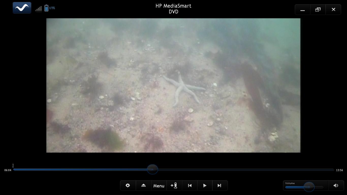 Fig 29
Unidentified rhodophyte
 Fig
30
Fig
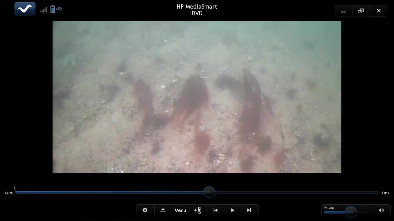
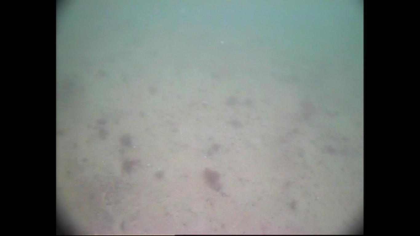
30Still 7:
Bare seafloor, little bedforms or macroalgae visible
 Fig
31
Fig
31Still 8: 11:50:14.136,182730.71,33813.56,0.00,0.00,0.00,324.8,-139.43,
Unidentified rhodophyte
 Fig
32
Fig
32Side scan analysis of three transects of the sea bed to the west of the port of Falmouth revealed 5 dominant bedforms, including a range of natural bedforms and a possible anthropogenic bedform.
Video and grab sample analysis were used to ground truth the side scan, identifying the main composition of sediment as maerl skeletons, providing a 3 dimensional habitat for many other marine species. The most abundant species present included Spirorbis spirorbis (polychaete), Liocarcinus holsatus (crustaceans), Ascidia conchilega (tunicate) and Echinocardium chordatum (echinoderm).
With a vast variety of marine life present in this area above and within a relatively dynamic seabed, the impact of dredging could cause great disturbance to marine flora and fauna.
The aim of the estuary survey was to sample at points from the marine end member up stream into the riverine dominated channel.
Sampling for nutrients (N,P,S) and oxygen at varying salinity allows us to create a estuarine mixing diagram and conclude whether nutrient concentrations are conservative or non conservative.
Biological activity, anthropogenic input and other processes may cause a nutrient concentration to plot below the theoretical dilution line showing non conservative behaviour.
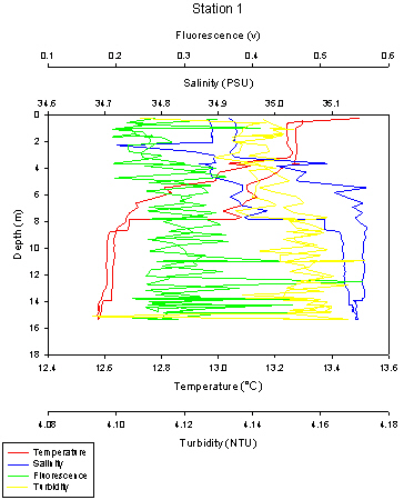
Station 1 was sampled down to approximately 15 metres. The temperature of the water column varies with depth, with surface temperatures recorded at 13.5oC whilst temperatures recorded at 15m were 12.6oC. This corresponds to the water types and the stratification present here, with the warmer and less dense riverine water laying over the more dense and cooler marine saline water.
The thermocline is visible from 4 to 6 metres at Station 1. There is also a halocline visible which corresponds with the thermocline, situated at 4-8 metres depth. The water at surface depths has a salinity of 34.92, however when it reaches the depths of the thermocline, at 4 metres there is an increase in salinity to 35.1. The salinity stays high here down to 8 metres, going above 35.1, showing the presence of the saline, denser water.
There is also a large difference noted between the ascending and descending casts of the temperature and salinity measurements from the CTD. Also, there are high chlorophyll values at the thermocline, which are determined using fluorescence as a proxy. The chlorophyll values at the thermocline are 0.35v and there is also another peak at 11 metres of 0.45v. Also at just past 12 metres, there is the largest chlorophyll value of around 0.57v.
Finally, turbidity also increases with depth, with turbidity maxima at the bottom. At the surface, the turbidity is 4.11 NTU and increases as you move down the water column to 4.17 NTU at 15 metres.
 Fig
33
Fig
33Station 2 was sampled down to approximately 20 metres. The temperature of the water column also changes with depth as seen in Station 1, at the surface there is highest temperatures of 14.4oC and the lowest temperature is at the deepest depth of 20 metres and is around 12.9oC. Once again, this corresponds to the stratification that is present in the water column at station 2, with the fresh, warmer water sitting at the surface and the colder denser water below this, with no mixing between the two layers of water.
The thermocline is very clear in Station 2, positioned at 5 metres, which is an area where the temperature rapidly changes. There is also a halocline present which corresponds to the thermocline, situated at 5 metres. The surface waters have a salinity of 34.0, but at 5 metres the salinity rapidly increases to 34.8, the salinity stays high down to depths of 20 metres, increasing more slowly to 35.0.
There is a smaller difference between the ascending and descending casts in comparison to Station 1, but should not be ignored. Also, there are high chlorophyll values at the thermocline, with a value of 0.52v. There is a large amount of noise in the chlorophyll plot, in that there is a lot of variability in the data with increasing depth. Finally, turbidity also increases with depth, similar to Station 1.
The turbidity maximum is also at the bottom of the CTD plot. At surface, the turbidity is 4.09 NTU and increases to 4.15 NTU at 20 metres, however there is also a lot of noise with the turbidity plot as you go down the water column.
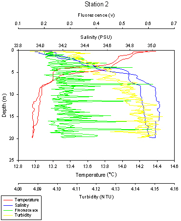 Fig 34
Station 3a was sampled down to 12 metres. The temperature of the water column once again changes with depth, with the highest temperatures at the surface of about 14.6oC and the lowest temperature is at the deepest depth of 12 metres and is around 12.9oC. This corresponds to stratification present in the water column, with a fresh layer sitting at the surface and a cooler denser layer below this. This means no turbulent mixing is occurring between these 2 layers. The thermocline is present at 2-4 metres.
There is also a halocline present, which corresponds to the thermocline. The salinity is 32.0 at the surface, but at the thermocline, between 2 to 4 metres, the salinity rapidly increases to 34.5. From this point, the salinity stays high, slowly increasing to 35.0 at 12 metres.
There is also another difference between the temperature and salinities from the ascending and descending casts of the CTD plot, so there is slight variation in the values seen. The chlorophyll values once again show a lot of noise, and are small at the surface, with a value of 0.2v, before there is a massive spike at the bottom of the CTD plot at 12 metres of 1.3v.
The turbidity maximum is once again at the bottom of the CTD plot. At surface, the turbidity is 4.00 NTU, and the turbidity gradually increases as you go down the water column, before reaching its maximum value of 4.10 NTU at 12
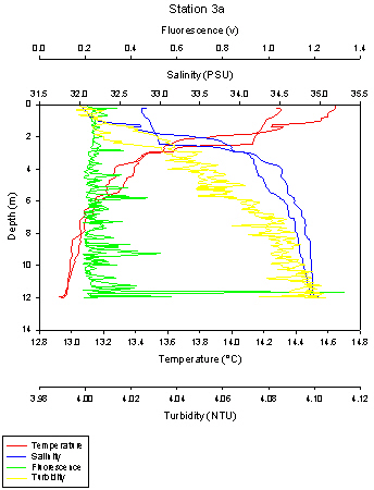 Fig 35
Station 3b was sampled down to 12 metres. The temperature of the water column changes with depth, with the highest temperatures seen at the surface before decreasing with depth. The temperature at the surface is 14.6oC and the lowest temperature is at the deepest depth of 12 metres and is about 12.9oC.
This corresponds to water stratification present, with no mixing occurring between the two layers of fresh and saline water. There is a strong thermocline present at 4 metres, and there is also a corresponding strong halocline. The salinity is 32.0 at the surface water, but at the thermocline of 4 metres, the salinity rapidly increases to 34.5. From this point, salinity once again stays high, slowly increasing to 34.9 at 12 metres.
There is also a difference at Station 3b between the salinities and temperatures produced from the CTD plot from the up and down casts of the CTD. The chlorophyll once again shows quite a lot of noise, and are small at the surface with a value of 0.2v. There are 2 chlorophyll spikes, one at 9 metres with a value of around 0.55v and the largest spike seen at 12 metres, with a value of 1.3v.
The turbidity maximum is once again at the bottom of the water column and the turbidity increases with depth. At surface, the turbidity is 0.2 NTU and the turbidity maximum is at 12 metres, with a value of 4.15 NTU.
 Fig 36
This means the most useful data in the centre of the channel has been lost in 2 of the 3 transects.
Transect 1
Mouth of estuary
Start position: LAT 050 08.565N LON 005 01.105W
Start time: 13:18:19 UTC
End position: LAT 050 08.599N LON 005 02.006W
End Time: 13:24:46 UTC
Surface (Q) of
-161.80m3/s
Bottom (Q) of -114.27m3/s
Total (Q) of -1738.32 m3/s
The first transect along of the estuary was taken at the mouth, ending at 231m from Black Rock.
Velocities are fairly constant throughout the transect either side of the channel, whereas the flow within the Carrick Roads had a general direction out of the direction. This is due to the ebb tide that was occuring during sampling.
The velocities are slightly slower on the East side of the river (right hand side of the ADCP plot) than the West side.
Data for the deep part of the channel was unobtainable as its depth is too great that the ADCP cannot register the backscatter information. Depth ranges from 9m to a maximum measured of 17m
Transect 2
Start
position:LAT 050 10.044N LON 005 02.787W
Start time: 13:44:29 UTC
End position: LAT 050 09.777N LON 005 01.628W
End Time:13:57:30 UTC
Surface (Q) of
-209.90m3/s
Bottom (Q) of -112.89m3/s
Total (Q) of -1034.89 m3/s
The second transect was taken further up the estuary, once again the
central channel is missing from the data due to the depth being too
great for the ADCP to register. Velocities remain slower towards
the banks of the channel and appear to speed up towards the centre
and at the surface. The lack of data however means that this cannot be
confirmed.
There are slightly slower velocities
recorded on one side of the river than the other, especially near the
bank, and close to the sides of the channel, showing friction reduces
velocities.
Transect 3
Start position: LAT
050 12.249 N / LONG 005 02.460 W 65m from shore
Start time: 15:01:06 UTC
End position: LAT 050 12.131 N / LONG 005 02.129 W 65m from shore
End time: 15:05:50
Surface (Q) of 64.81m3/s
Bottom (Q) of 37.02m3/s
Total (Q) of 328.69 m3/s
Surface flow maximum of 0.565m/s
Minimum flow 0.010 m/s
The shallower depth allowed a full transect to be retrieved showing in greater detail the separation of velocities from the surface waters within the channel and the bottom waters. The flow is greatest in the surface waters of the channel, 0.565m/s, as a result of input from freshwater sources combining with the outgoing tide to increase the flow velocity.
The deep water incorporating most of the volume of the channel had a much slower velocity of 0.010m/s, showing that tidal currents are much slower than river currents. Friction slows the flow in the deep water and close to the bottom and banks.
Flow direction is still towards the mouth of the estuary, as we remained on the ebb tide.
The CTD on-board the Bill Conway, which was used for the estuary sampling did not have a density recorder attached, which is a key component in the Ri number equation. Due to this, a programme had to be used to calculate the density from the salinity, temperature and depth recordings from the CTD.
This means that there is a slight error involved as we are calculating the density ourselves rather than having a direct output from the CTD. The ADCP transect was used in accordance with the CTD data to be able to work out the Ri number, as the ADCP records the velocity of the current.
| Transect No. | Group | Time (UTC) Start/End |
LAT (N) Start/End |
LON (W) Start/ End |
Ri No. |
| 1 | 4 | 13:18:19/13:24:46 | 50o08.565/50o08.599 | 05o01.105/05o02.006 | 1.128 |
| 2 | 4 | 13:44:29/13:57:30 | 50o10.044/50o09.777 | 05o02.787/05o01.628 | 1.058 |
| 3 | 4 | 15:01:06/15:05:50 | 50o12.249/50o12.131 | 05o02.460/05o02.129 | 3.452 |
| 4 | 11 | 08:32 | 50o14.390 | 05o00.940 | 2.063 |
| 5 | 11 | 09:27 | 50o13.676 | 05o01.030 | 1.005 |
| 6 | 11 | 10:40 | 50o12.256 | 05o02.461 | 6.999 |
The Ri numbers for the Group 4 stations are all quite similar, all being larger than 1. Station 1 has a Ri number of 1.128, Station 2 has an Ri number of 1.058 and Station 3 has an Ri number of 3.452. Station 3 has a slightly larger Ri number, but all of the Stations are above 1, which means that the water here is stratified and no mixing is occurring.
The Ri numbers for the Group 11 stations are also similar and are all larger than 1. Station 4 has a Ri number of 2.063, Station 5 has a Ri number of 1.005 and Station 6 has a Ri number of 6.999.
Although Station 6 has a much larger Ri, which could suggest an extremely strongly stratified water column, all of the stations from Group 11 have an Ri number larger than 1 and so the water columns here are all stratified with no mixing occurring.
Overall, the Estuary Sampling has shown, from the Richardson Numbers that the waters are stratified and no mixing is occurring. This is to be expected as in the Estuary there is an influx of saline and river water.
Due to the differences in density of these two water bodies, i.e. saline water is denser due to the increased concentrations of salts and minerals, which mean it is denser and sinks below the fresh river water.
This causes a stratified water column, with fresh water at the surface and saline water below this layer, with no mixing between the two, which is represented by the Richardson Numbers calculated above.
Nitrate concentrations are highest at the riverine end member of the estuary with the highest concentration being 38.8µM at salinity of 0. The lowest concentration observed was 0.7M at a salinity of 35.3.
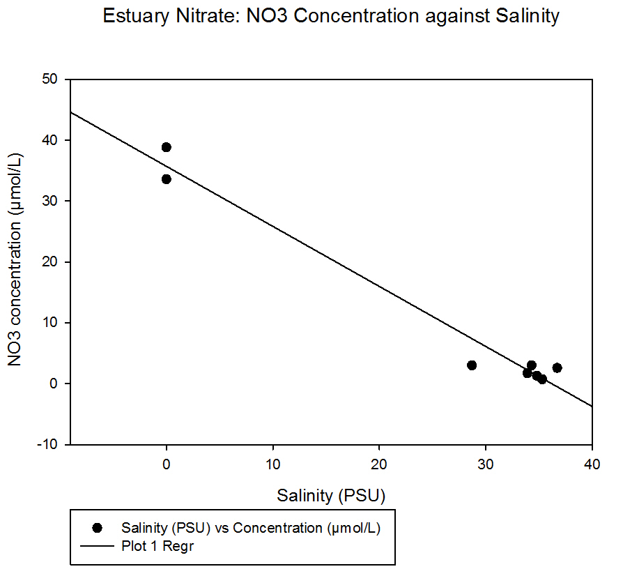 fig 40
Looking at the TDL it appears that phosphate mainly occurs at different concentrations at high salinities. The regression line added to the graph suggests that with decreasing salinity the concentration of phosphate increases; however as most of the data points are between the salinity ranges of 30-40 a larger range of salinities is needed to confirm this.
Generally the data taken from higher up the estuary has a slightly lower salinity and a slightly higher concentration of phosphate than the data collected further down the estuary.
The river end members were taken from the two different rivers
that feed the estuary, each of these was measured twice to make
sure they were accurate.
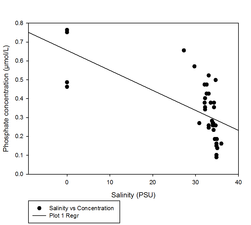 Fig 41
This graph shows the four end members from the top of the river along with data collected up the estuary by group 11 and data collected at the bottom of the estuary by group 4.
It is clear that with increased salinity the concentration of silicon decreases, however the lowest salinity point is 28.7 meaning that there is a large range of unknown values for salinity and concentrations.
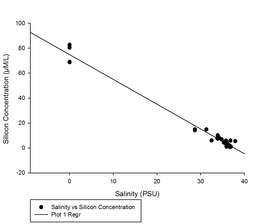 Fig 42
Generally the results show a weak trend line of increased chlorophyll with decreasing salinity. However the correlation is not very strong as not all of the points lie close to the line, and there are varying concentrations for the same salinity value.
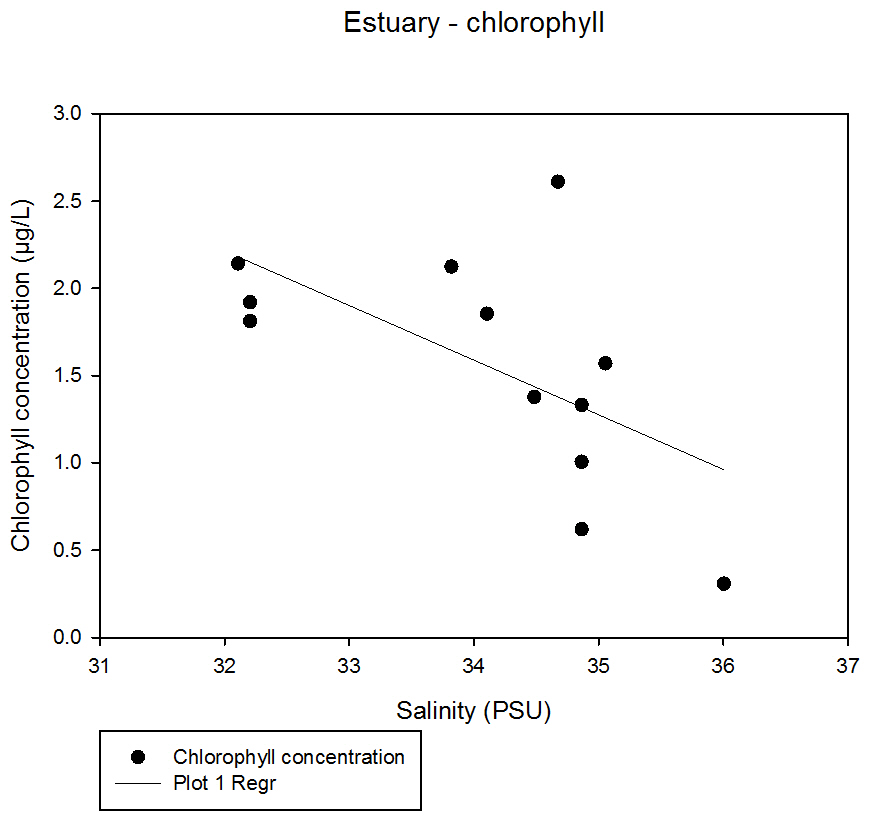 Fig 43
The graph shows that there is no obvious observed correlation between oxygen saturation and salinity in the estuary from our samples taken.
The highest value of oxygen saturation obtained was 109.10% at a salinity of 34.87 and the lowest saturation value was 96.52% at a salinity of 34.49.
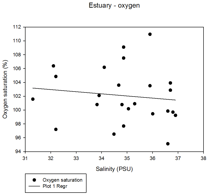 Fig 44
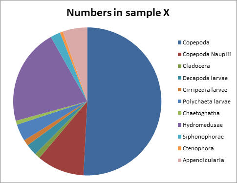
Similarly to the offshore stations, the two zooplankton samples collected show that copepods were the dominant zooplankton group, showing proportions of 51% for the first station and 49% for the second station. At both stations both Copepod Nauplii and Hydromedusae made up large proportions of the zooplankton.
Copepods have also been found to be the dominant zooplankton group in the estuary by data recorded by the NERC Western Channel Observatory.
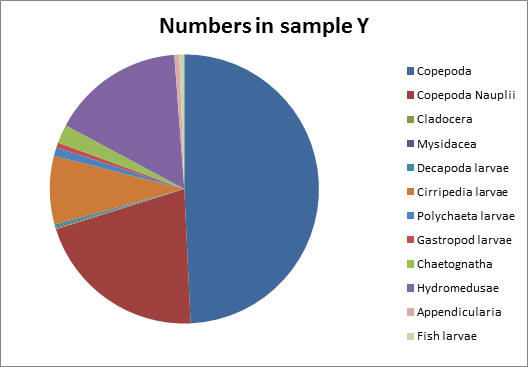
Sample Y taken further towards the head of the estuary showed a significant proportion of Cirriped larvae that was absent at the mouth of the estuary.
This suggests that juvenile barnacles are adapted to tolerate lower salinities in comparison to adults which tend to be found in coastal regions.
Sample X showed that copepods were the dominant group of zooplankton at the mouth of the estuary, likely due to their fast growth rate. They are known to be important in the food web of the area, as they serve as a food source for many fish and other invertebrates (Gotto, 1979).
They feed by moving their limbs and antennae to create vortices around the body, and then use appendages called setae to collect food particles that have been drawn in by the feeding currents (Koehl and Stickler, 1981).
Hydromedusae also made up a significant proportion of the total zooplankton, of 21%. A reason for this is that they also feed on phytoplankton (Brusca and Brusca, 2003), and at this time of year resources are not limiting.
Finally, copepod nauplii had a significant prescence, showing that copepods are able to reproduce, develop and mature at the mouth of the estuary. This may be lower than the proportion in sample Y as some Nauplius larvae will get washed out to sea despite having swimming appendages (Brusca and Brusca, 2003).
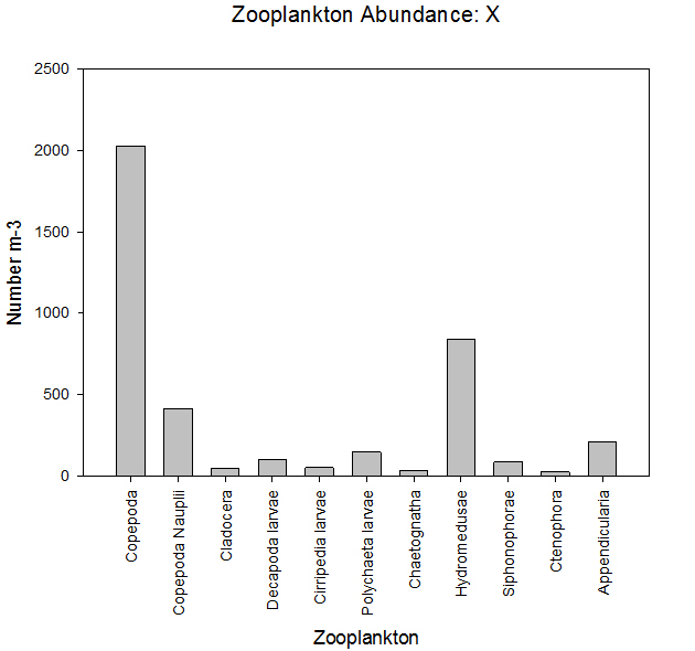 Fig 45
 Fig
46
Fig
46
Sample Y, taken further up the estuary showed that copepods were still the dominant zooplankton group making up 49% of the sample. Copepod nauplii made up the second highest proportion, of 21%, and the number of individuals per litre counted was similar to sample X. Hydromedusae (jellyfish) again made up a notable proportion (16%) of the total zooplankton.
Like copepods, many species feed on phytoplankton and suspended particles in the water column, although overall there is a lot of variation in feeding habits. Some hydromedusae show prey selection and feed on fish larvae and soft bodied crustaceans like copepods. They feed by stunning and trapping organisms using stinging cells on their tentacles called nematocysts (Brusca and Brusca, 2003).
Hydromedusae are drawn to large concentrations of prey as they are sensitive to chemicals given off (Purcell, 1997). Finally, sample Y shows a distinct amount of Cirriped larvae of 10%, compared with a much smaller amount found in sample X of roughly 1% of the total zooplankton in the sample.
This possibly shows that the environment here is more tolerable for juvenile barnacles than at the mouth of the estuary (Gotto, 1979). However, to be more confident about the distribution of zooplankton along the estuary, we would need to take zooplankton samples at a lot more stations at varying salinities. Our data may also be affected by counting errors and misidentification of species.
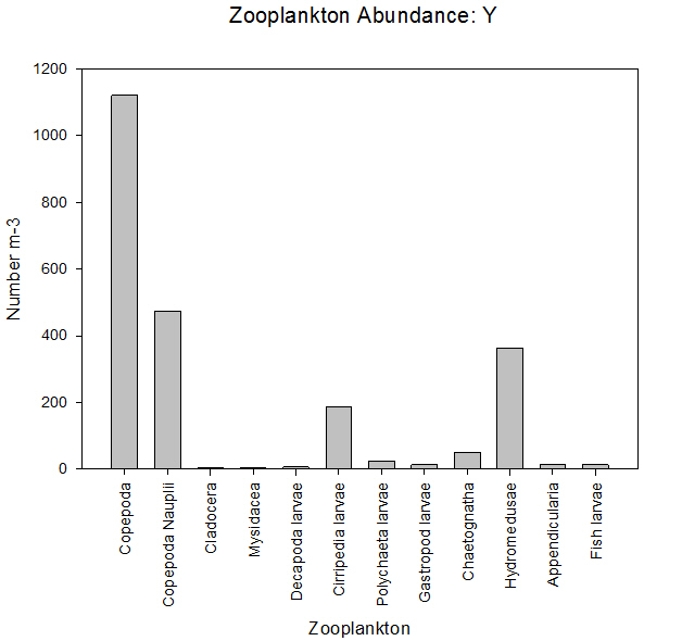 Fig 47
 Fig
48
Fig
48
|
|
Cells/L |
||
|
Species |
Station 1 |
Station 2 |
Station 3 |
|
Alexandrium |
|
240000 |
30000 |
|
Guinardia flaccida |
130000 |
20000 |
70000 |
|
Guinardia striata |
920000 |
120000 |
120000 |
|
Rhizosolenia alata |
30000 |
|
30000 |
|
Rhizosolenia imbricata |
10000 |
20000 |
20000 |
|
Rhizosolenia setigera |
120000 |
60000 |
70000 |
|
Ceratium fusus |
20000 |
|
|
|
Chaetoceros |
90000 |
30000 |
40000 |
|
Eucampia |
|
|
20000 |
|
Leptocylindrus danicus |
120000 |
|
10000 |
|
Pseudo-nitzschia |
150000 |
|
|
|
Nitzschia |
|
10000 |
20000 |
|
Total |
Total Cells/L |
||
|
Diatoms |
1570000 |
260000 |
400000 |
|
Dinoflagellate |
20000 |
240000 |
30000 |
The identified species were organised into tables for each of the stations. All of the species we identified were either diatoms or dinoflagellates and the table lists all of the species present and the estimated number of cells per litre at each station.
Station 1 showed a large proportion of diatoms (98.7%) within the phytoplankton sample, with Guinardia striata making up the majority of the total composition. This diatom has many small chloroplasts and forms curving cylindrical cells that appear as spiralling chains under the microscope (Tomas, 1997).
At the second station there appeared to be an even distribution of diatoms and dinoflagellates, making up 52% and 48% of the overall phytoplankton composition. However this is due to a large abundance of the dinoflagellate Alexandrium which was the only dinoflagellate identified, and it had a cell count of 240000 per Litre. Alexandrium populations tend to peak in spring in temperate waters with high nutrient concentrations (Anderson, 1998), and can form harmful algal blooms which cause paralytic shellfish poisoning (PSP) (Lilly, 2003). This could possibly be either the build-up or the deformation of a harmful algal bloom, but further studies would need to be done to confirm this.
Station 3 appears to show similar results to station 1, in terms of plankton distribution. The diatom count was 400,000 cells per litre (97%) whereas the dinoflagellate count was much lower at approximately 30,000 cells per litre (3%). Again Guinardia made up a large proportion of the overall phytoplankton count, due to their rapid reproduction rate (Horner, 2002).
Another diatom, Rhizosolenia also made up a large proportion of the diatoms present. These cells tend to be straight or slightly curved, and generally are solitary. They can form aggregations of cells clustered in parallel in rapidly growing populations (Round et. al, 1990).
In summary, apart from an unusual bloom of Alexandrium, diatoms were the dominant group of phytoplankton at each station in the estuary. This is due to them not being limited by nutrients such as silica, and because they have a faster growth rate then dinoflagellates (Horner, 2002).
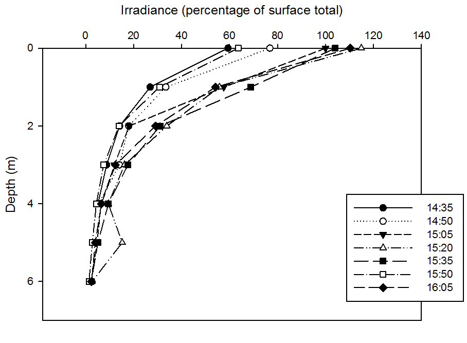
This graph is expressed as the percentage total of surface-in-air irradiance so as to eliminate the problem of variation in cloud cover and other external variables and thus making each time station directly comparable. This graph shows that overall, irradiance decreases exponentially with depth, which is because of the rapid attenuation of light, especially of the longwave red wavelengths in the surface layers. It also however shows a general trend of increasing irradiance with time, which is likely due to the fact that we were taking the samples during a flood tide in a strongly tidal estuary, and thus the marine inputs were gradually becoming more influential during the sample time period. As fluvial inputs generally have greater light attenuation values due to higher suspended particulate matter and thus low light irradiance values, as the marine influence increases, irradiance values will also increase.
Two anomalies are evident in this data however, firstly, and most obvious at a first glance, is the 5m value at 15.20BST, where the irradiance increases significantly to 9.32%. The second anomaly is the entire line plotted from 15.50BST. Although most of the data follows the trend of increasing irradiance with time, this series bears data much lower than expected, notably in the surface layers (0-1m). On reflection, we have realised that although this shouldn’t be attributed to variation in variables such as cloud cover and insolation due to calibrating and making the data a percentage of the surface air irradiance, if there was a lag between taking the reading and a cloud passing over for example, this would cause discrepancies.
As it is unlikely that a sudden change in irradiance due to a natural in situ phenomena such as resuspension of sediment, and this is especially unlikely to reach the surface layers, we have named the possible cause as the result of a strong tidal flood tide current having been taking the probe away from the pontoon at each time, and this particular time, it may have been slightly submerged under the pontoon itself. It is also possible that a piece of debris, natural or man-made, such as macroalgae, of which there was a significant amount of Fucus vesiculosus in the area, may have entangled itself around the probe, blocking some irradiance. However, another very plausible reason would be due to the patchiness of the water column, and thus the possibility of a water mass of difference properties becoming trapped.
 fig
49
fig
49The natural log of percentage total surface irradiance was taken for each depth. The log irrandiance with depth graph forms a straight line when plotted, showing that the proportion of light decays exponentialy with depth.
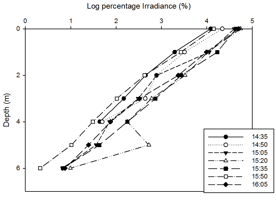 fig 50
This graph shows that at each time, salinity always increases with depth. However, it must be noted that the halocline decreases less significantly as time goes by. The greatest salinity change with depth is found at 14.35BST, where it increases from 30.57 at the surface to 32.38 at 4m depth. The significant increase in salinity at depth at the earlier stations is due to the earlier flood tide being in the process of salt-wedging the estuary’s water column, however, as the lenses of freshwater on the surface due to fluvial input and terrestrial run-off change, the buoyancy and hence turbulence, which increases mixing and thus increases the halocline gradient.
It can be seen that there is again an anomaly in this data set, at 16.05BST at 3m depth where the salinity increases significantly. This could be due to human error, but is again more likely to be due to the patchiness experienced in water columns such as this.
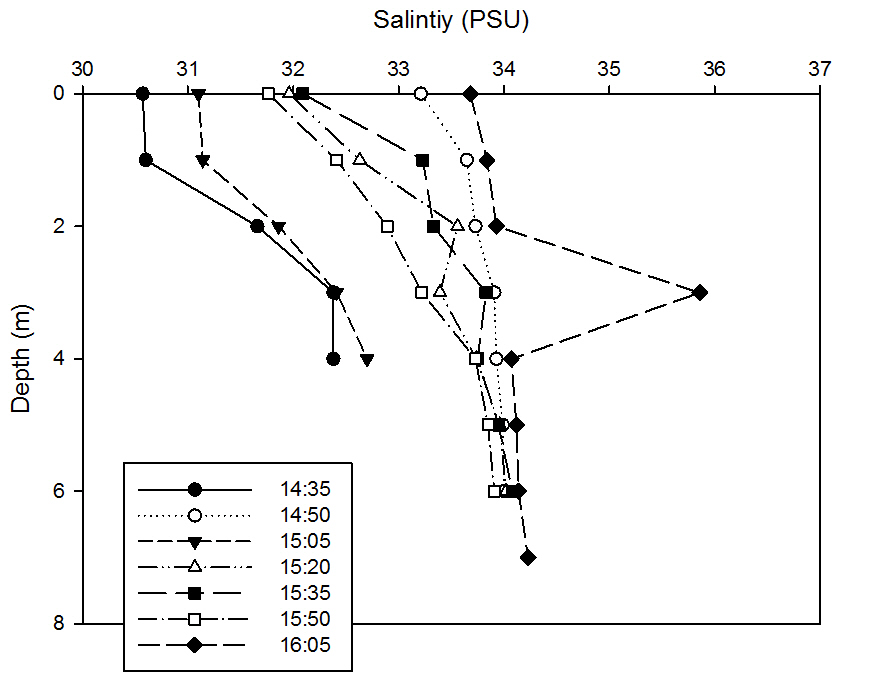 fig 51
This graph shows that dissolved oxygen levels are decreasing with depth, which is mostly due to phytoplankton, but also other organisms at depth assimilating the dissolved oxygen for respiration. However in reference to time, there are less obvious patterns when compared to the other variables measured. It can be seen for the first three times sampled, that dissolved oxygen saturation levels increase with increasing time, which is likely due to increased marine inputs refreshing the dissolved oxygen levels this far up the estuary.
It can then be seen that later time samples become less saturated, which could either be due to assimilation by flora and fauna in the water column or increased mixing. A feature of this plot that is interesting however is the fact that the maximum saturation for the earlier times between 14.35BST and 15.05BST are at around 1m depth whereas after 15.20BST, maximum saturation is pushed down to 2m depth.
This is likely due to the fact that the salt-wedging causes a boundary which pushes up the water mass present, and so the maxima is higher when this phenomena is occurring at the earlier stages during flood tide until it begins to mix and push down nearing high tide.
This also corresponds with the higher and more rapidly decreasing oxygen after the maxima chlorophyll values at earlier times and the less pronounced and lower maxima at later times in the chlorophyll plot.
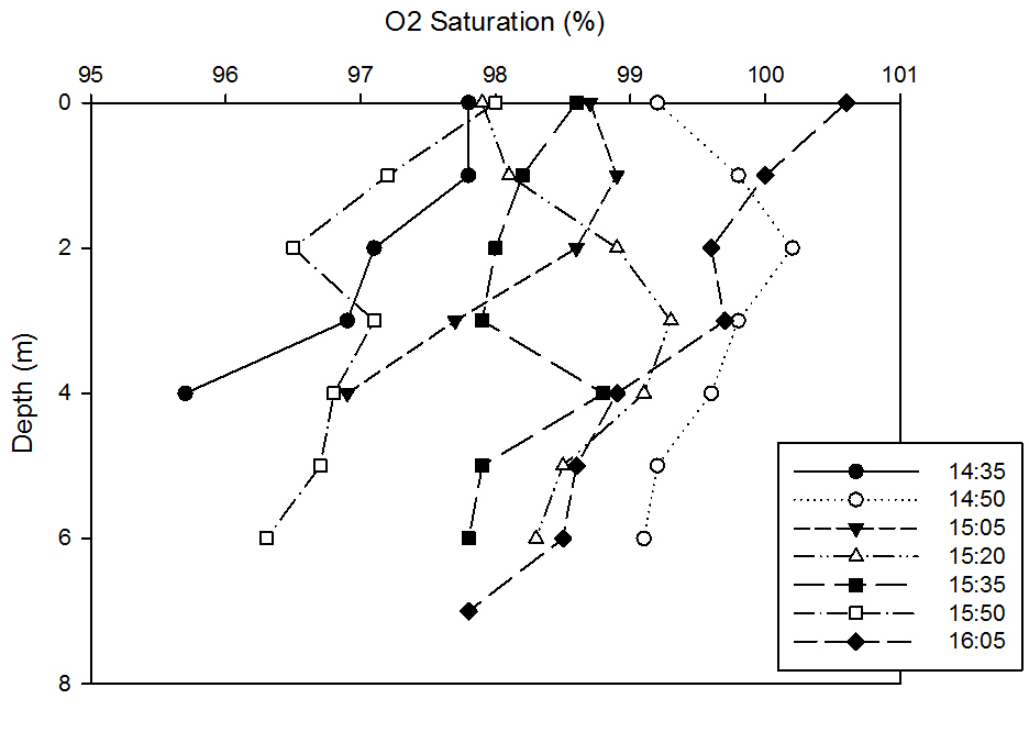 fig 52
This graph shows that there is a gradual decrease in water temperature with increasing depth, with the maximum increase being around 0.6°C at 15.35m. This is due to the greater attenuation of light at the surface warming these upper layers of the water column and less heating of lower layers, thus, due to the colder water being denser, it sinks to the bottom. It can also be seen that over time, the water temperatures of the entire profile decreases, from a surface maximum of 15.05°C at the earliest time of 14.35BST and a minimum surface value of 14.33°C 16.05BST.
This is due to the increasing marine influence of colder waters as we approach high tide. It can also be seen that it becomes a less pronounced thermocline over time as it reaches high tide. This is likely due to the fact that at the earlier flood tide period of the tidal cycle, the estuary will be salt wedging, where colder, denser marine waters will be pushing underneath the warmer, less dense fluvial lenses of freshwater overlying these water masses. These profiles become less pronounced as the water column becomes gradually more marine influenced and the salt wedge pushes further up the estuary and becomes increasingly well-mixed.
An anomaly can be noted on this graph - the last value at 7m depth at 16.05BST where temperature significantly increases from 14.09°C at 6m to 15.05°C at 7m, which is equivalent to our highest surface value of our very first time series. After careful consideration, it could be a possibility that the YSI probe may have slightly touched the sediment or entered the turbulent boundary layer of densely suspended sediment, as the operator remembers there being difficultly accurately monitoring the depth of the probe, due to the location on the depth gauge and the very significant lag time between actual depth and the depth that appears on the YSI data output screen.
We know that sediment holds onto heat for longer than water due to possessing a higher specific heat capacity and depending on porosity, which is likely here to be minimal due to the presence of muds, are not flushed rapidly, presenting a time lag between properties noted in the sediment and those changing more rapidly in the above water column.
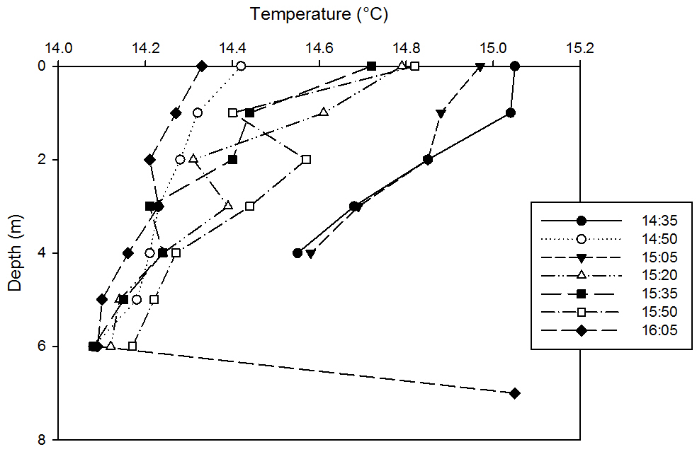 fig 53
Although we would expect pH values to increase with increased marine input, this graph illustrates that the YSI probe used is not likely to be precise enough to measure such small fluctuations in pH, due to the great variation experienced in the plots.
However, for the majority of the earlier plots, it can be seen that at depths beyond 4m, where the marine influences lie according to the salinity profiles, pH decreases, and by the time the water column is well mixed around high tide at 16.05BST, the pH profile remains at a constant value of 8.67 from the surface to 7m.
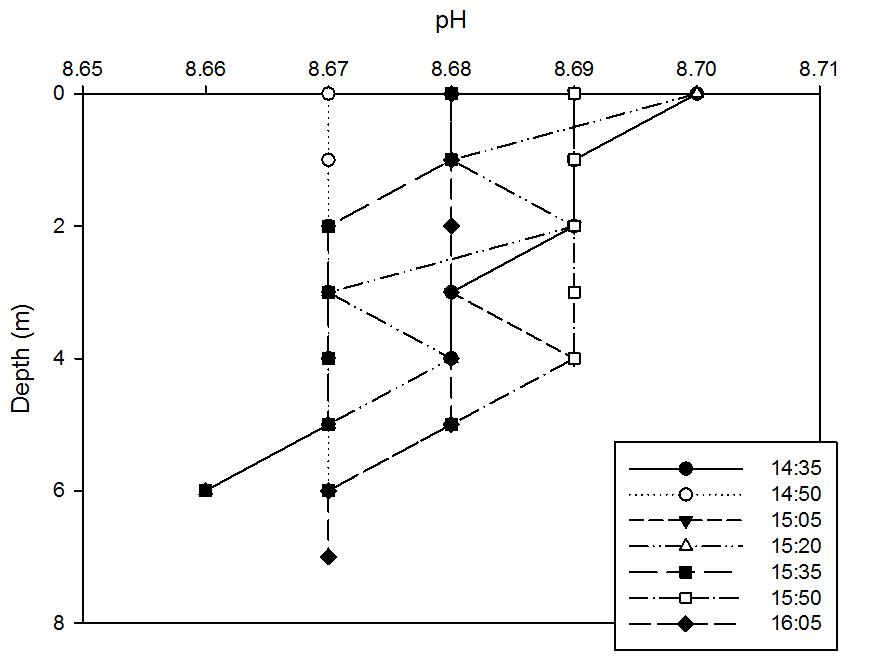 fig 54
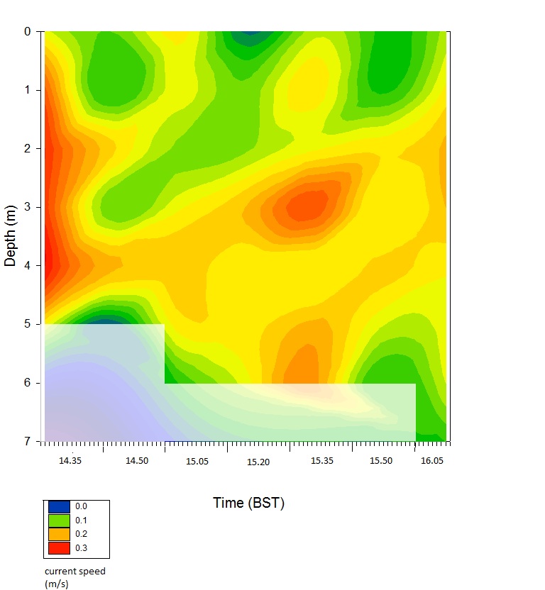
This graph shows that at that as time increases, and thus time towards high tide and slack water, the current speed decreases. The highest speeds are at 14.35BST of 0.28m/s at 2m and decrease significantly after this time up until 16.05BST.
The surface current speeds are lowest due to the marine inputs causing the high current flows are entering at deeper depths due to salt wedging caused by the denser properties of this water mass. The flood tide begins to slow as the tidal influence decreases. It can be seen between 15.20BST and 15.35BST that there are higher current values around 0.29 m/s at 3m and continuously anomalously high throughout the water column at this time, which is likely due to a non-natural effect such as the wake of a passing boat.
It should be noted that the blocked out area is due to the fact that sigmaplot during plotting the contour plot, it tried to interpolate and extrapolate the data where we did not go down to depths covered by this zone as the water levels were not high enough.
 fig
54a
fig
54a
The data collected
within the Fal represents a stratified estuary, as demonstrated
by the Richardson numbers, which are all above 1 indicating that
no mixing is occurring.
From the data collected it can be seen that there is a general
trend across the three stations, with significant
characteristics differentiating them as we move further up the
estuary, towards the riverine source.
Sampling up the estuary showed a thermocline at depth for station 1, at Black Rock, at 6-7m.
The thermocline can be
seen to move higher up the water column as we move closer to the
fresh, cooler riverine inputs, to a depth of 5m at station 2 and
2-4m at station 3. Also shown in
the CTD data there is a corresponding halocline, to the
thermocline, at corresponding depths, 6.5 and 2m up the estuary.
As expected salinity decreases up the estuary, due to inputs
from freshwater sources, from 34.9 at the surface of station 1,
34.0 at station 2 and 32.7 at station 3.
Turbidity was found to
increase with depth. Turbidity decreased with movement up the estuary
from a maximum at the mouth.
The flow of the estuary is greatest at the surface of the
central channel.
The results for nitrate show highest concentrations at the
riverine end member, however most of the samples collected were
below detection for nitrate.
Silicon is behaving conservatively, with decreasing
concentrations with increasing salinities.
Phosphate proved to be very variable at high salinities, plotting above and below the TDL. The lack of mid salinity data doesn’t allow for an overall picture of the behaviour of phosphate within the estuary. The variability of phosphate could be a result of the high agricultural, sewage and mine drainage runoff into the Fal (Matthiessen, 2001).
Measurements of O2 saturation show oxic conditions throughout the estuary, so this is not a limiting factor. There is no obvious correlation between oxygen saturation and salinity. Chlorophyll concentrations were found to be decrease out of the estuary; however this conflicts with the increase in phytoplankton out of the estuary seen within the net samples taken. Only three samples were taken, however, so it was difficult to quantify.
Phytoplankton samples show a trend of diatoms being the dominant group within the estuary. Silica is not limiting but it is notably lower at higher salinities. Diatoms require silica for impregnating their cell wall, known as a frustule. The species found tended to have low silica content according to descriptions suggesting that these can tolerate low silica concentrations better than other diatoms. One genus of dinoflagellate, Alexandrium, was prevalent at station 2, possibly due to its ability to move throughout the water column to utilise high concentrations of nutrients.
Copepods were found to be dominant species of zooplankton; likely as these tend to feed on the phytoplankton which are prevalent at this time of year. This dominance of copepods was also seen in data collected by the NERC Western Channel observatory. Large numbers of hydromedusae in sample X could be a response to high populations of copepods, as they are drawn to chemicals given off by large concentrations of their prey.
On the day of our survey (29/6/12) weather conditions were poor with high winds and rough sea surface conditions with large waves (south west, force 4-6 with 1m plus waves within the harbour). This restricted the safe working area we could survey in and forced us to stay within the sheltered water relatively close to shore behind the shelter of the peninsular.
We still managed to survey towards the edge of the estuary and survey the mouth of the Helford river to the West of the Fal estuary.
The strong wind had a impact on internal waves which could be seen in our vertical CTD profiles. The strong wind and surface current also made it difficult to stay exactly on the station when collecting data, this drifting is likely to effect results.
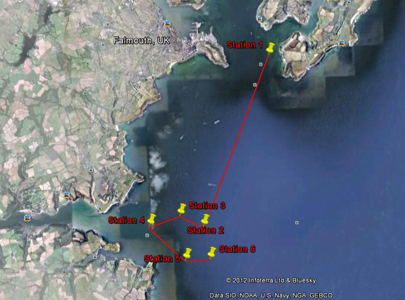
Figure 43 shows the Offshore survey station postions.
 Fig
55
Fig
55At station 1, both oxygen saturation and chlorophyll concentration decrease linearly with depth. For chlorophyll, values decrease from 1.27 to 0.88µg/L between 6 and 27m respectively. The oxygen saturation of the water column decreases from 97.78 to 91.31% between 6 and 27m respectively.
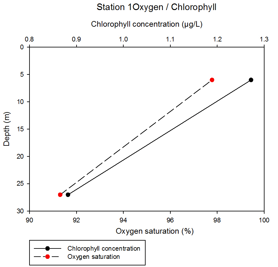 fig 56
At station 2, chlorophyll concentration decreases linearly with depth, decreasing from 1.83µg/L to 1.07µg/L between 2 and 21m sampling depth. Oxygen saturation increases between 2 and 8m, from 98.59% to 105.65% before decreasing to 95.92% at 21m.
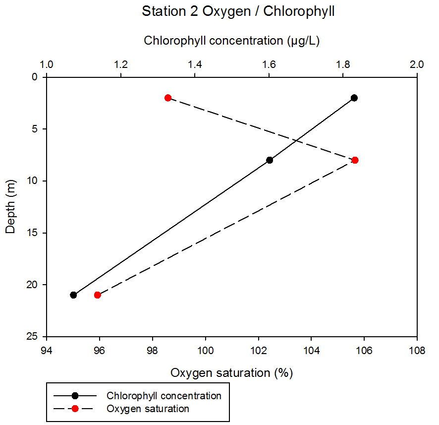 fig 57
At station 3, chlorophyll concentration decreases between 1.5 and 6 m from 1.54 to 1.24µg/L before increasing to 1.73µg/L at 11.5m. Oxygen saturation decreases with depth but not linearly; between 1.5 and 6m values decrease from 95.06 to 88.79%, whereas between the 6 and 11.5m depth, values decrease more dramatically to 86.72%.
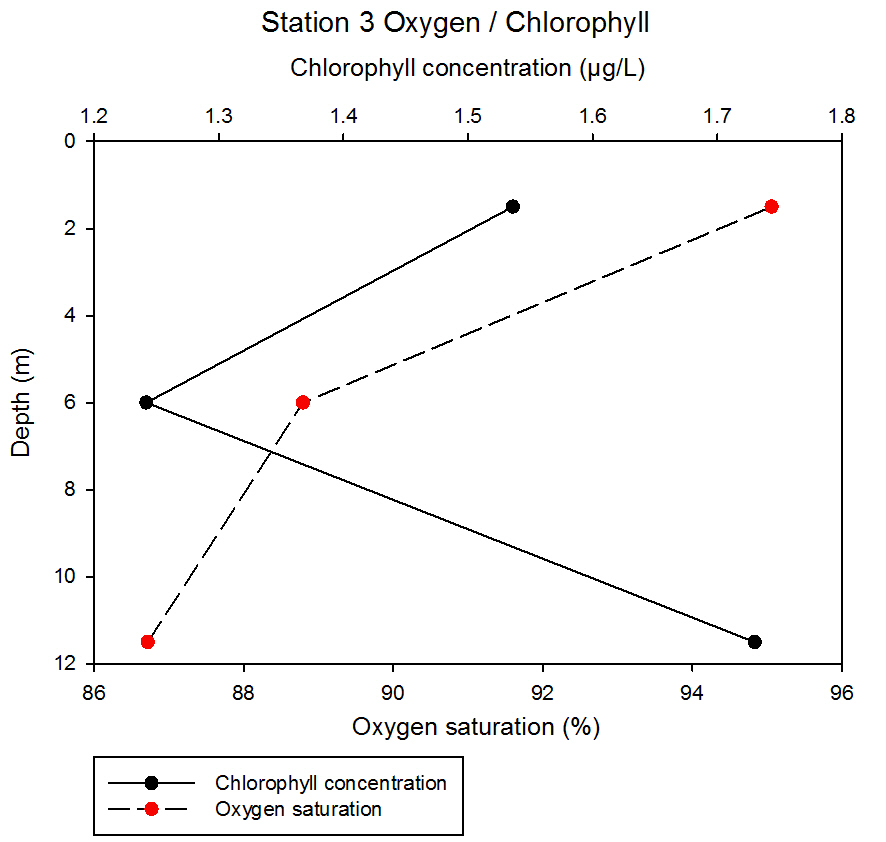 fig 58
At station 4, oxygen saturation decreases linearly, with saturation values decreasing from 97.04 to 81.30% between 2 and 7.5m. Chlorophyll concentration increases between 2 and 4.5m from 1.44 to 1.86µg/L before decreasing to 1.76µg/L at 7.5 metres depth in the water column.
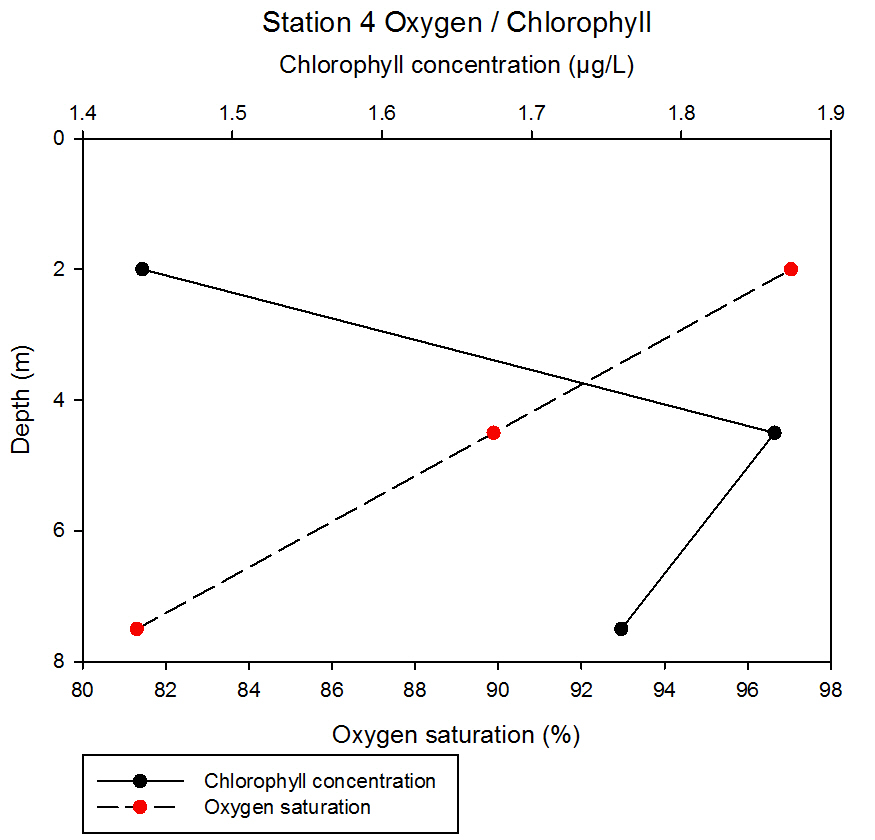 fig 59
At station 5, chlorophyll concentration and oxygen saturation appear to show an inverse relationship. Between 3 and 9m depth, oxygen saturation decreases from 101.42 to 77.37% and then increases between 9 and 13m depth to 82.18%. Chlorophyll concentration contrasts this; increasing between 3 and 9m from 1.10 to 1.42µg/L before decreasing dramatically between 9 and 13m to 0.43µg/L.
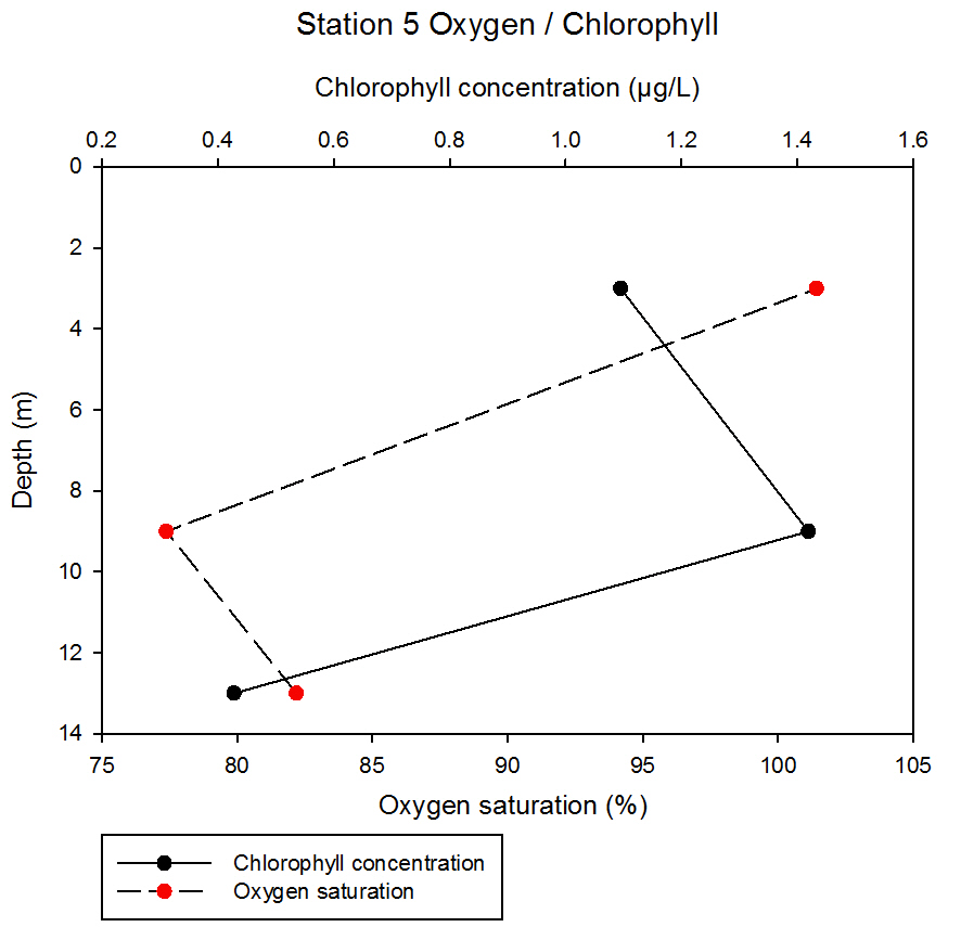 fig 60
At station 6, chlorophyll concentration decreases between 3 and 8m from 1.70 to 0.61µg/L before increasing to 1.91µg/L at a 15m depth. The value at 15m depth for this station was the highest chlorophyll value obtained from our readings taken. The oxygen saturation increased slightly between 3 and 8 metres depth from 100.05 to 102.85% before decreasing quite dramatically between 8 and 15m to 87.05%.
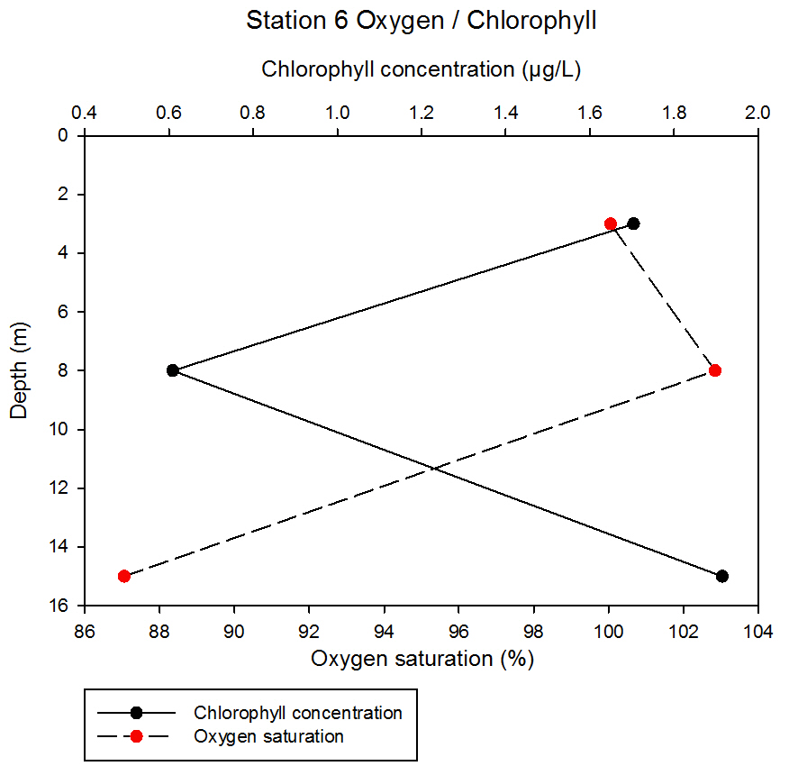 fig 61
There does not seem to be a relationship between oxygen saturation or chlorophyll concentration at the different stations. The highest chlorophyll concentration was obtained at station 6 at 15m depth with a reading of 1.91µg/L. The lowest chlorophyll concentration was obtained at station 5 with a reading of 0.43µg/L. Station 5 also shows the lowest oxygen saturation, with a reading of 77.37%. 105.65% was the highest oxygen saturation reading, which was obtained at station 2.
At station 1, the data show a contrasting pattern of nutrient concentration with depth. The shallowest sampling depth of 6m contained silicon with a concentration of 1.21µmol/L which increased by 0.35µmol/L at the second sampling depth of 27m, measuring at 1.56µmol/L. Phosphate shows a less dramatic change in concentration with depth, although decreases from 0.098 to 0.129µmol/L from 2m to 27m.
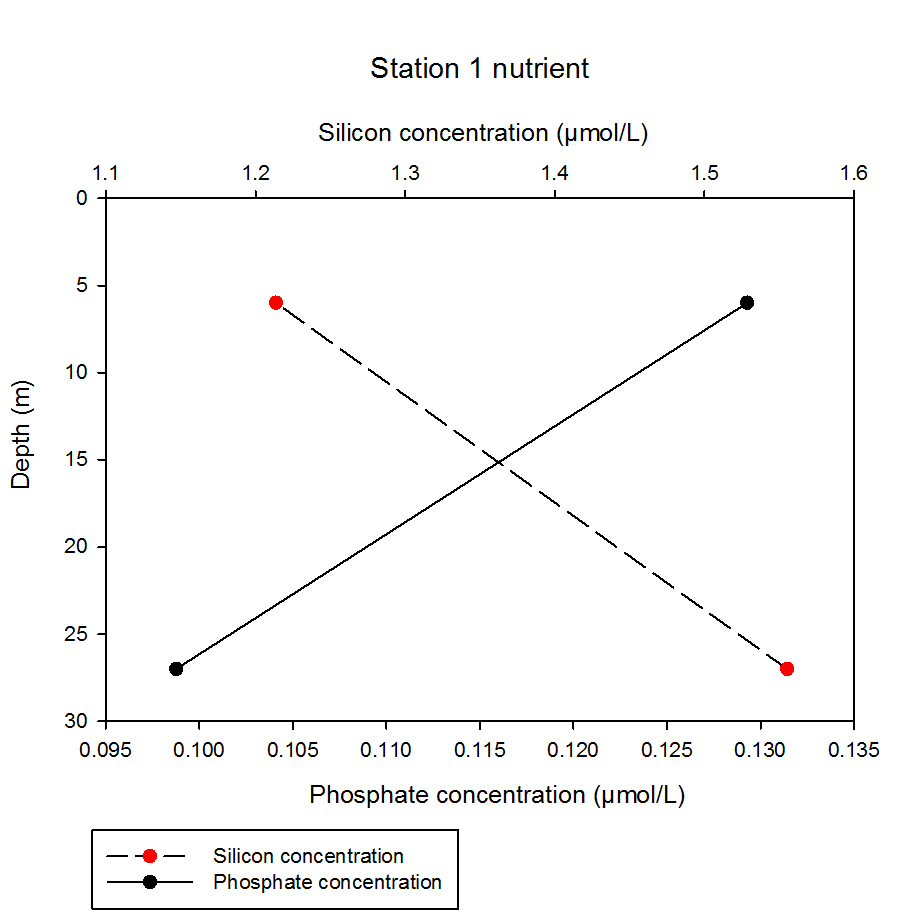 fig 62
At station 2, both silicon and phosphate concentration show a general increase with depth, whereas the results for nitrate do not show a clear cut increase with depth. Silicon increases linearly with depth, inclining from 1.00 to 1.59µmol/L at depths 2m and 21m respectively. Phosphate shows an initial decrease in depth from 2m to 8m measuring at 0.062 and 0.056µmol/L respectively, and then increases dramatically to 0.117µmol/L at 21m. Nitrate notably contrasts the patterns of silicon and phosphate, where it dramatically decreases from 2m to 8m from 1.5 to 1.3µmol/L, and then increasing to 1.3µmol/L at 21m.
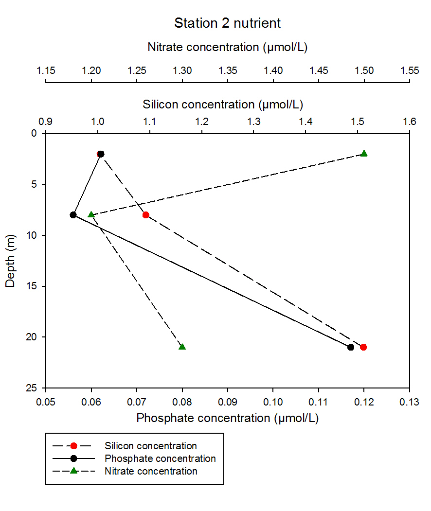 fig 63
At station 3, silicon consistently increases with depth from 1.39 to 1.40µmol/L from 1.5m to 6m, and then a dramatic increase to 1.56µmol/L at 11.5m. Phosphate initially decreases with depth from 0.123 to 0.093µmol/L at 1.5 and 6m respectively. This concentration then increases to 0.129µmol/L at 11.5m, which is similar in concentration to the measurement obtained from the shallowest sampling depth of this station.
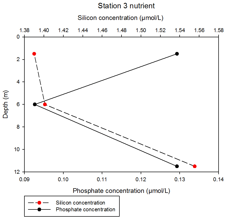 fig 64
At station 4, the data show contrasting results for silicon and phosphate concentrations. Silicon consistently increases with depth, with an initial increase of 0.05µmol/L between 2 and 4.5m, measuring at 1.42 and 1.47µmol/L at 2 and 4.5m respectively. Phosphate consistently decreases with depth, sharply declining between 2 and 4.5m from 0.18 to 0.13µmol/L respectively, and then further declines to 0.12µmol/L at 13m. Data for only one sampling depth was obtained for nitrate, measuring at 1.3µmol/L at 13m.
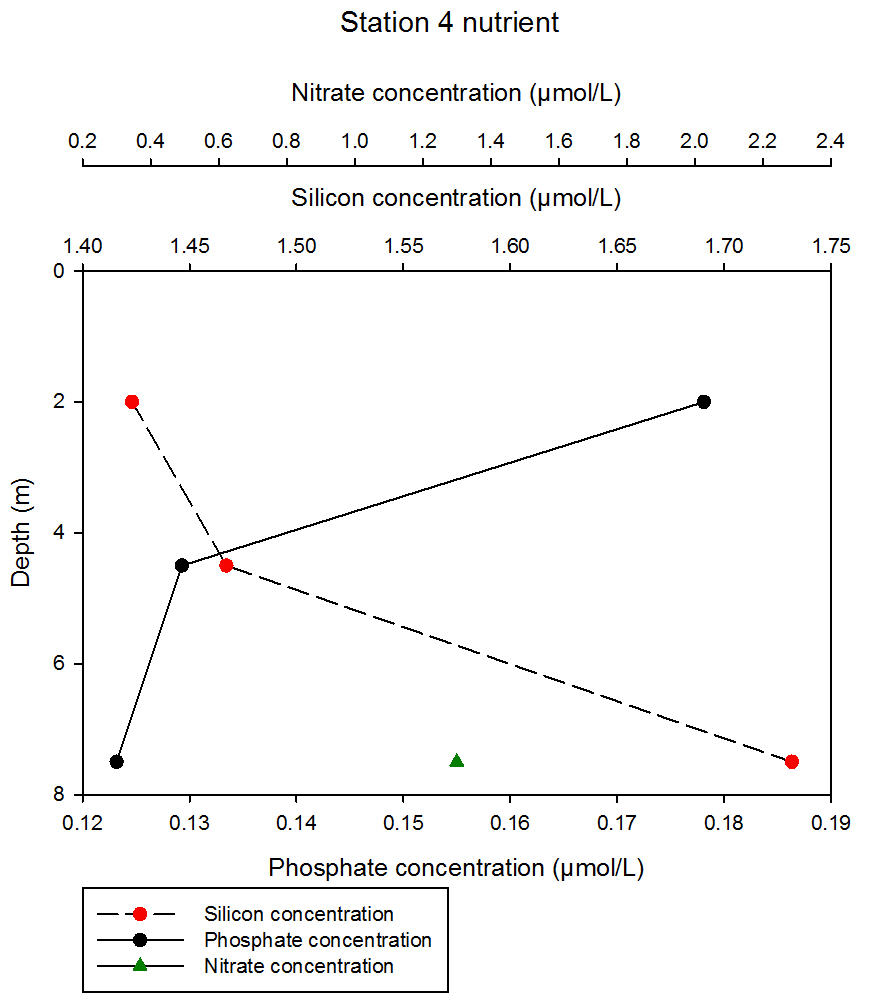 fig 65
At station 5, the data show similar depth profiles of silicon and phosphate, both of which increase with depth. Silicon measures at 0.74µmol/L at the shallowest sampling depth of 3m, which increases to 1.97µmol/L at 13m. Phosphate shows a similar rate increase with depth, albeit in weaker concentrations, increasing from 0.12 to 0.28µmol/L from 3 to 13m.
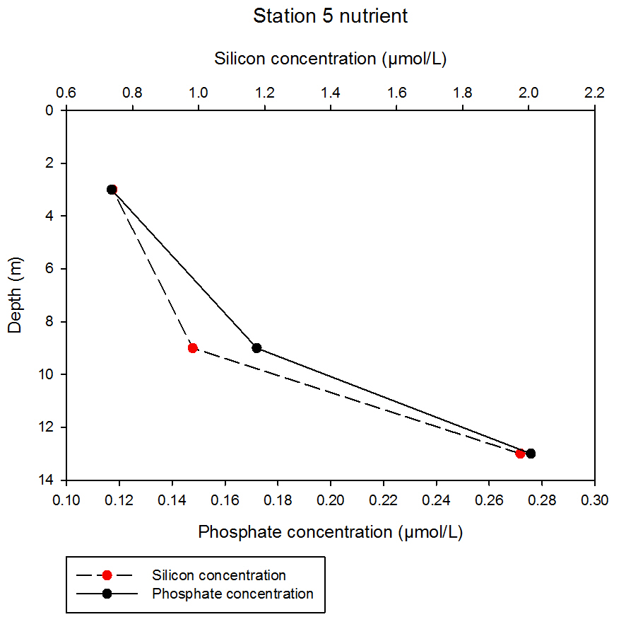 fig 66
At station 6, silicon shows a consistent increase with depth, with an initial increase of 0.18µmol/L between sampling depths at 3 and 8m, measuring at 0.41 and 0.59µmol/L respectively. A sharp increase of 1.23µmol/L then occurs by sampling depth 15m, measuring at 1.82µmol/L. Phosphate initially decreases with depth from 0.09 to 0.02µmol/L, but then increases dramatically to 0.17µmol/L at 15m.
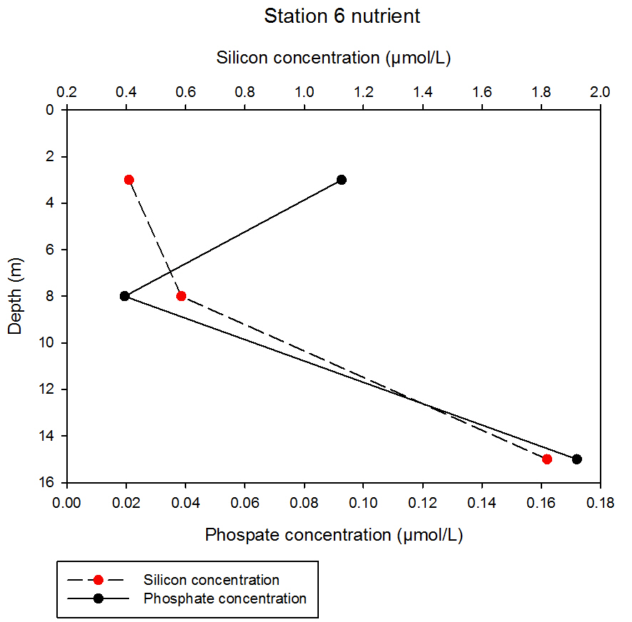 fig 67
The data for silicon and phosphate concentrations throughout all stations show varying results, although it can be seen that silicon remains at a consistently higher concentration than phosphate throughout all depths. Station 5 exhibited the highest concentration of silicon and phosphate throughout all stations, measuring at 1.974 and 0.276µmol/L respectively, both of which were obtained at the 7m sampling depth. Station 6 exhibited the lowest concentrations of silicon and phosphate, measuring at 0.409 and 0.019µmol/L respectively, obtained from sampling depths 3 and 8m respectively. Data for nitrate was only obtained for station 2 and at one sampling depth at station 4 due to practicalities of accuracy and precision in the wet lab onboard RV Callista, as most samples obtained were below the detection limit of the equipment used.
At each station we estimated the relative abundances of different groups of zooplankton in the water column. To do this we deployed a 50cm diameter plankton closing net to a set depth, then raised it up to a known depth to analyse a specific part of the water column. We closed the net by sending messenger weights down the line once we got to our required depth. These triggered the release of a mechanism that closed the net, allowing us to sample a known volume of water. The net had a 200 micrometre mesh allowing us to extract zooplankton from the water column and collect them in 1L sampling bottles. 10ml of Formalin was added to each bottle in order to kill the zooplankton so that the consistency of the sample would not change whilst stored before analysis.
The next day we took the samples from each station and extracted 5ml of sample and placed it within a Bogorov chamber in order to count the amount of zooplankton under a light microscope. This process was repeated so 10ml of sample was analysed for each station. We grouped the fauna by order/group and tallied the results in a table for each station and depth range. The species were identified using the book Coastal Plankton: Photo Guide for the European Seas by Otto Larink.
In order to estimate the relative abundance of zooplankton in the water column, we needed to calculate the volume of water we had filtered. We multiplied the distance (change in depth in metres), by the area of the phytoplankton net. Then to work out the number of individuals per litre, we divide the number of animals of a specific order/group, by the number of litres sampled.
Results and discussion
We collected zooplankton data at 6 stations, and at different depths, taking eight samples in total. For the majority of the offshore stations, we found that copepods were the dominant group of zooplankton.
At stations 1, 2, 3 and 6 copepods made up the mass majority of the individuals recorded. Station 1 was at the mouth of the estuary and showed the highest proportion of copepods in the zooplankton sample, of 90%.
Only the station 4 sample taken from 8-2m did not show copepods as the dominant group. Instead both copepods and decapod larvae showed similar proportions, of 21% and 24% respectively.
Other groups that made up significant amounts of the zooplankton included Appendicularia, Copepod Nauplii and Hydromedusae. Due limited time, it was not possible to do multiple repeats and it is possible some species were incorrectly classified.
The observations of Copepods being the dominant zooplankton group are supported by several studies, both locally (Western Channel Observatory-NERC) and globally (Dürbaum & Künnemann, 1997). These studies also report that copepods form the largest proportion of biomass marine systems.
Station 1.
Copepods dominate here at Blackrock at the mouth of the estuary. They make up 90% of all the zooplankton present in the sample and have a count in excess of 100,000 individuals per litre.
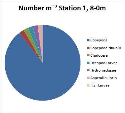 fig 68
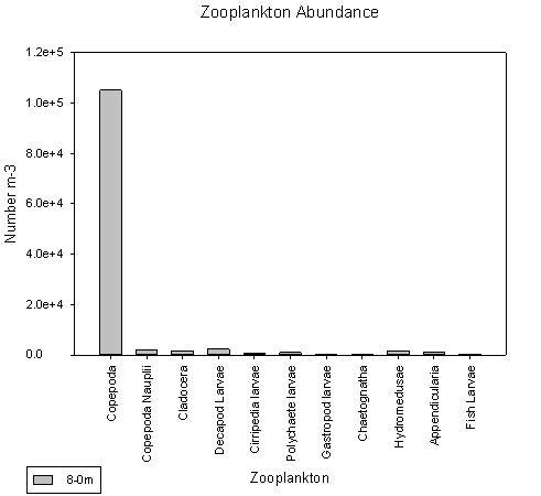 fig 69
Station 2, 7-2m
Copepods make up around 54% and decapod larvae 35% of the total zooplankton population according to the adjacent pie chart. Copepods have an approximate count of around 7000 individuals per litre.
Station 2, 15-10m
Copepods dominate here again, with approximately 8000 individuals per litre. As can be seen from the pie chart they make up 42% of the overall zooplankton. Compared to other stations, a wider variety of zooplankton groups of is present.
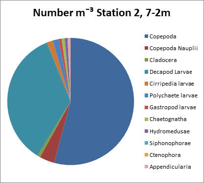 fig 70
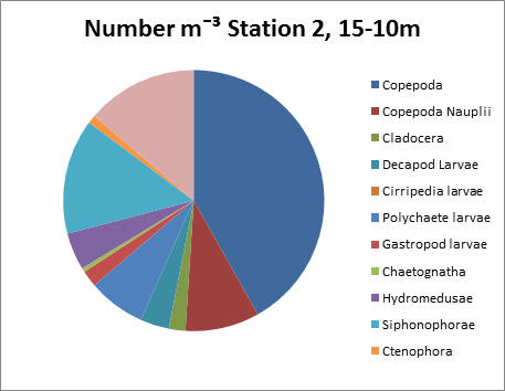 fig 71
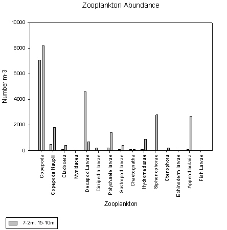 fig 72
Station 3, 15-7m.
This sample shows significantly lower zooplankton counts than at 6-2m. Copepods still dominate with a count of 1000 per litre, and hydromedusae are second most prevalent with a count of 500 per litre approximately.
Station 3, 6-2m
Station 3, 6-2m has a much larger overall zooplankton count than the deeper sample at this station. Copepods dominate with an approximate count of 9000 per litre.
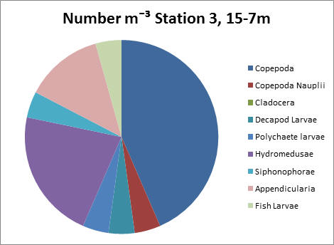 fig 73
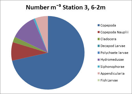 fig 74
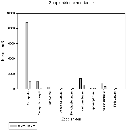 fig 75
The station 4 sample taken from 8-2m did not show copepods as the dominant group. Instead both copepods and decapod larvae showed similar proportions, of 21% and 24%, and counts of approximately 600 and 700 individuals per litre, respectively.
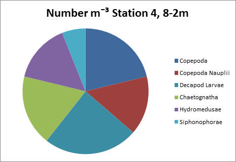 fig 76
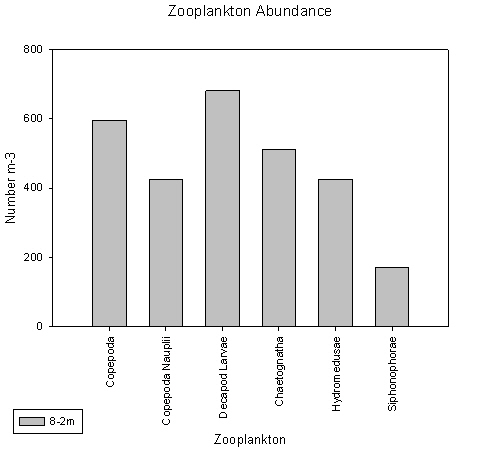 fig 77
At Station 5 copepods and nauplius larvae were found to dominate, as can be seen in both graphs. Copepods have a count of 3400 individuals per litre and their larvae have a total count per litre of 2500 individuals.
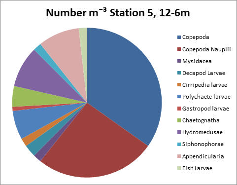 fig 78
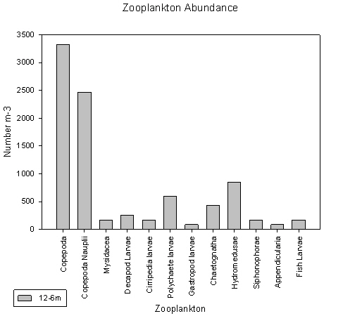 fig 79
Station 6 shows a deep chlorophyll maxima, which is typically formed during periods of prolonged stratification (see ADCP and CTD data). Copepods dominate, as both graphs show, with a count of 2200 per litre.
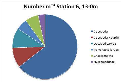 fig 80
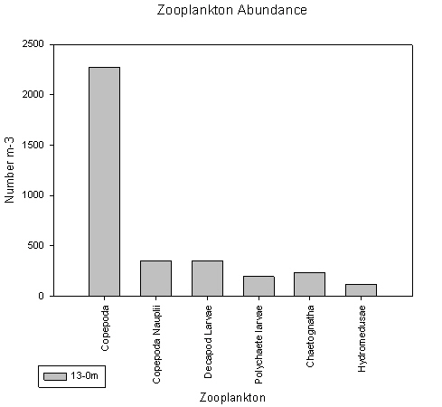 fig 81
In total we took 17 phytoplankton samples, 2 at station 1, and 3 at each of the other stations. For station 1 we did not record the depths on the Niskin bottle deployments, but we noted the depths for all of the other samples collected. Station 1 was Blackrock (Same as the estuary), in both the shallow and deep samples, diatoms made up the mass majority of the phytoplankton recorded.
As in the estuary sample at this station, Guinardia striata is the most abundant species at both depths. This diatom has many small chloroplasts and forms curving cylindrical cells that appear as spiralling chains under the microscope (Tomas, 1997).
Station 2 showed similar trends to station 1 at all depths as diatoms, particularly Guinardia, were dominant. At 8.2m the cells/ml is twice that of 2.3m and 4 times greater than at 20.8m.
This suggests that this is the optimal depth for maximising phytoplankton growth in the water column. In other words phytoplankton are not too deep to be light limited and not too near to the surface in nutrient limited waters (Round et. al, 1990).
Station 3 shows a similar trend with depth to station 2, in that the middle value of 6.2m has a significantly larger proportion of phytoplankton than the surface or deeper reading of 11.5m. The consistency of phytoplankton is also similar to station 2 as diatoms, particularly Guinardia, dominate due to its rapid reproduction rate.
Station 4 shows similar trends to 2 and 3; at 7.5m there is a peak in phytoplankton for which the majority is the diatom Guinardia. There are some dinoflagellates present, as either Alexandrium, or Ceratium fusus; however these only made up around 3% of the overall phytoplankton composition.
Station 5 again shows that diatoms are dominant due to a large proportion of Guinardia in the overall phytoplankton count. Station 5 differs from the previous three stations as the phytoplankton distribution at all three recorded depths is relatively similar. This suggests that irradiance and nutrients do not become limiting from 2.7m to 13.3m in the water column.
As station 6 has a similar trend to all the other offshore stations we can conclude several things about our data. Guinardia particularly G. striata is the dominant species of phytoplankton off the coast of Falmouth.
The distribution of phytoplankton is relatively constant throughout the water column, suggesting nutrients are well mixed and that there is little stratification. Other diatoms have a significant prescence at particular depths, at 15.1m Pseudo-nitzschia makes up roughly 25% of the total phytoplankton, but has limited distribution in shallower waters.
Dinoflagellates will begin to dominate later in the year once diatoms start to be limited by silica which they need for their cell walls. Diatoms such as Guinardia are able to dominate as they require very little silica compared to other diatoms (Horner, 2002).
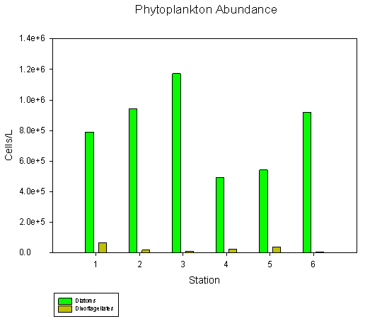 fig 82
LAT: 050 08.816N
LON: 005 01.395W
Station 1 was sampled to a depth of 28m and can be seen to have a clear thermocline at 10m and a second less obvious thermocline with two noticeable steps at 10m and 16m, with a halocline also present at these depths.
The relationship between chlorophyll and irradiance in the surface layer to an approximate 3m depth can be seen. There are low chlorophyll values in the top 3m despite high irradiance. This may be due to photoinhibition caused by exposure to high light intensities, where damage to the light harvesting pigments prevents efficient conversion of photons into chemical potential energy, and so depriving the plant of an energy source for healthy growth.
There is a slight peak in the chlorophyll value just above the first thermocline depth at approximately 8m of 0.125v, as phytoplankton, due to its limited mobility, exists usually above the thermocline to avoid being mixed down below where there is sufficient nutrients and light for photosynthesis.
It should be noted however that there is a significant amount of noise on the fluorometer reading, but both the ascending and descending profiles follow a relatively constant profile.
The separation of ascending and descending profiles, particularly temperature and salinity is likely due to the presence of internal waves in the water column moving the water masses and their constituents up and down, as described below in the internal waves section.
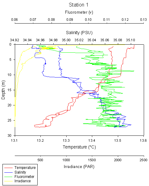 fig 83
Time:09:54 UTC
LAT: 050 05.729N
LON: 005 03.221W
Station 2, sampled to a depth of 22m. A thermocline can be seen at 17m and 14m, however there is a very large variation in the ascending and descending cast of temperature, i.e. the position of the thermocline.
This is evidence for the presence of internal waves, which have propagated along the pycnocline in the time between the ascending and descending cast and caused the variation that can be seen on the plot.
Irradiance decreasing with depth due to increased light attenuation, but also a large difference between the up and down cast.
Chlorophyll concentration increases below the surface layers due to decreased photoinhibition. There is a chlorophyll maximum at 14m which coincides with the thermocline, where we would expect nutrient concentrations to be high. Phytoplankton need to stay in the stratified water to prevent them being mixed to depths below the thermocline and out of the high irradiance of the surface waters.
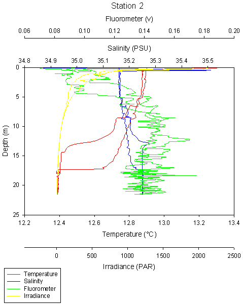 fig 84
Time:10.59 UTC
LAT: 050 05.919N
LON: 005 03.881W
Station 3 could be an example of a salinity spike near the surface at 1m depth.
The lag time between the temperature probe response and the calculation of salinity from conductivity and temperature can cause discrepancy seen in the surface salinity profile above 1m.
We would expect data from 0-1m to be of low quality and would tend to ignore this in our analysis. The CTD requires a short time to adjust to the water before good quality data can be recorded. The rest of the profile from 2-16m looks more like the profile which would be expected.
However, temperature and salinity readings are both very high at 1m depth and it would be wrong to remove the data from our graph. It could be a layer of stratified warmer water sitting on the surface, perhaps where there are low tidal currents and mixing, allowing it to reach slightly higher temperatures and salinities than other stations.
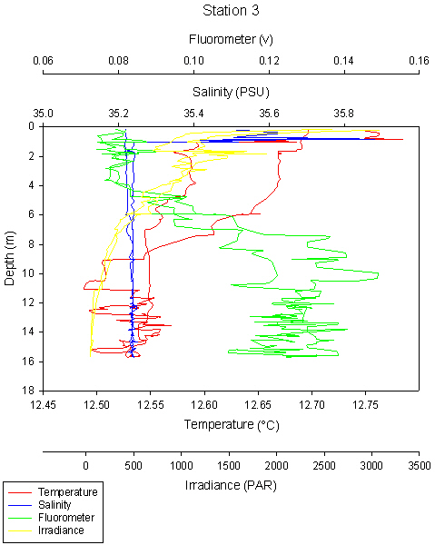 fig 85
Time:11.59 UTC
LAT: 050 05.733N
LON: 005 04.728W
This station was different to the other offshore stations, as we only sampled to a depth of 8m, which is less than the depth of the thermocline at the other five stations (1,2,3,5,6).
This was because we were in shallow water of less than 10m. No obvious thermocline can be seen because the water is shallow and well mixed preventing a thermocline forming. Tidal currents cause friction against the bottom, mixing the water column and overcoming any thermal stratification caused by irradiance.
Salinity spikes can be seen at the surface at 0-1m, with very high temperature and salinity. A weak thermocline can be seen at 6m, but it is not clear enough to be certain it is a thermocline.
The salinity spike at the surface is likely to be an anomaly as the spike only shows up on one of the CTD casts, similarly with temperature the two casts show high variability.
Chlorophylll maximum is at 8m and another peak at 4m.
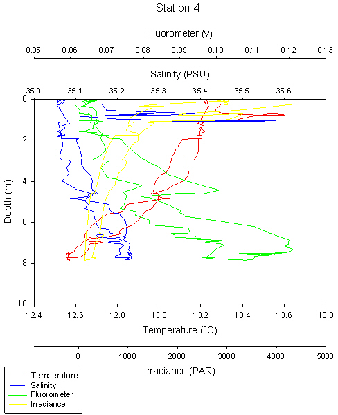 fig 86
Time:12:43 UTC
LAT: 050 05.116N
LON: 005 03.724W
Similarly to the other stations, data at the surface shows a lot of noise and should be ignored at 0-1m.
There is a double thermocline visible at 8m and at 11-14m. This can be seen on the plot as two steps in the decrease of temperature with depth. Interestingly, the salinity plot stays constant with depth with no halocline visible.
There is a large variation between the ascending and descending cast of irradiance and chlorophyll. One irradiance cast shows the expected logarithmic plot, whereas the other shows a much lower irradiance at the same depths. I would expect this to be an error, or possibly the CTD drifted through some disturbed, highly turbid water.
Chlorophyll is highest at the thermocline at 8-14m and increases with depth from the surface.
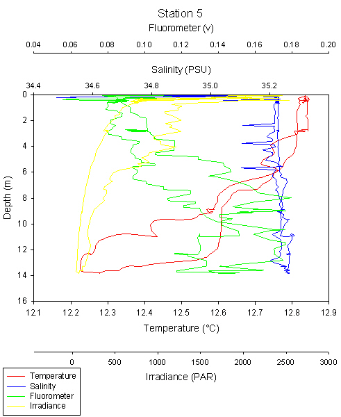 fig 87
Time:13:20 UTC
LAT: 050 05.136N
LON: 005 03.039W
The up and down casts seem to agree more at this station than others.
There is a double thermocline visible at 7m and 12m, with a halocline visible at both these depths, showing stratified fresher, warm water on top of colder more saline water.
The chlorophyll maximum can be clearly seen at 12m, with chlorophyll decreasing above and below 12m.
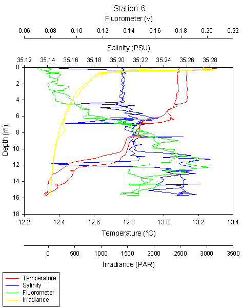 fig 88
| Station | Compensation Depth (m) |
| 1 | 19.91 |
| 2 | 17.07 |
| 3 | 15.27 |
| 4 | 10.50 |
| 5 | 16.73 |
| 6 | 16.06 |
See raw files for calculation table.
There tends to be a thermocline present at 8- 14m in all the stations, however there is a lot of variation in this value between the upcast and downcast, and between stations. There are two possible explanations for this; firstly, internal waves propagating along the thermocline causing the thermocline to change depth, and secondly, strong currents (wind and/or tide driven) causing the boat to drift whilst the CTD profiling was in progress.
Internal waves can be identified by the difference in the temperature plot on the down and up cast. The internal wave has propagated in the time the CTD has moved up and down causing the two plot lines to be different. This shows the thermocline has moved. The movement of the internal waves is driven by gravity in the same way as surface waves.
Strong onshore winds cause seawater to accumulate against a coastline due to Ekman transport and stokes drift. This water cannot continue to accumulate, gravity causes it to return back to its normal height down the pressure gradient. As this happens internal waves form on the thermocline/pycnocline where there is a density difference.
These waves are different to surface wave because the density difference between the two water masses is relatively small compared to a surface wave. This causes their amplitude to typically be larger than a surface wave.
Transect 1
Start position: LAT 50⁰06.207 N / LONG 005⁰03.630 W
Start time: 10:42 UTC
End position: LAT 50⁰05.744 N / LONG 005⁰04.888 W
Surface Q: 477.21 m3/s
Bottom Q: 285.41 m3/s
Total Q: 3543.36 m3/s
Velocity is greatest at the start of the transect, towards the east, as you move into deeper
waters, at the surface, 0.283m/s. The slowest velocity was
recorded towards the
end of transect, in the
shallow waters at the surface, 0.025m/s. Flow at the surface,
477.21 m3/s is greater than flow at the bottom,
285.41 m3/s, with a total flow over the transect of
3543.36 m3/s.
Start position: LAT 50°05.844 N / LONG 005°04.622 W
Start time: 12:44 UTC
End position: LAT 50°05.054 N / 005°03.754 W
End time: 12:44
Surface Q: -379.77 m3/s
Bottom Q: -240.21 m3/s
Total Q: -2634.51 m3/s
A bedform of an approximate height of 8m, can be seen and the effects it has on flow velocity
is clear. Flow velocity is greatest at the surface waters above
the bedforms and high velocities can be seen
surrounding the bedform,
Transect 3
Start position: LAT 50°05.610 N / LONG 005°03.337 W
Start time: 1:14 UTC
End position: 50°05.139 N / LONG 005°03.038 W
End time 1:20 UTC
Surface Q:
-145.24 m3/s
Bottom Q: -96.39 m3/s
Total Q -1261.77 m3/s
Looking at the three transects, flow appears to be decreasing. Total Q transect 1,2,3, 3543.36 m3/s,
-2634.51 m3/s, -1261.77 m3/s respectively,
as we move further away from the Fal estuary and riverine
inputs, also the cause of greater surface to bottom velocities,
and general flow out of the estuary caused by the ebb tide, seen
across the transects.
However as we were unable to reach greater distances from the shore, due to poor weather conditions, we are unable to make a comparison to see how much this differs further offshore.
The Richardson Number looks at the stratification of the water column at different points to take into account how stable the water column is.
It is a measure of the relative importance of the effects of mechanical and relative density in the water column, which are used to model instability driven by sheared flows.
Ri = g(Ρ1-Ρ2)h / (Ρ*u2)
Where
Ri = Richardson Number
g = Gravity
Ρ1 = Lowest Density
Ρ2 = Highest Density
h = height (depth of water)
Ρ = Average Density
u2 = Velocity.
When Ri is small, then velocity shear is considered sufficient to overcome the tendency of a stratified water column to stay stratified, so some mixing should occur.
When Ri is large, turbulent mixing will not occur and the column will tend to remain stratified.
If Ri is less than 0.25, water column is stable. If Ri is greater than 1, water column is unstable.
The Richardson number determines whether a water column is stratified or not.
|
Transect 1 (End Station 3) |
|
|
Depth (m) |
Ri |
|
2.58 |
0.280731 |
|
3.58 |
0.792081 |
|
4.58 |
0.849441 |
|
5.58 |
2.000813 |
|
6.58 |
0.564065 |
|
7.58 |
0.403786 |
|
8.58 |
0.316495 |
|
9.58 |
0.278528 |
|
10.58 |
0.374466 |
|
11.58 |
0.214547 |
|
12.58 |
0.206154 |
|
13.58 |
0.36239 |
|
14.58 |
0.482709 |
|
15.58 |
0.483468 |
Transect 1 was taken from 10:45 UTC to 10:59 UTC, with a start latitude of 50o05.728N and longitude of 005o03.23W and an end latitude of 50o05.929N and an end longitude of 005o03.930W.
Transect 1 shows low Richardson Numbers from surface depths of 2.5 metres to 4.58 metres.
These low Richardson numbers mean that the water column between these depths and more likely to overturn any stratification and to be mixing.
At a depth of 5.58, there is a much larger Ri number of 2.000813, which could coincide with the fact that this is the thermocline, which means that the water here is thermally stratified and mixing does not occur.
Below this depth to the lowest depth of 15.58 metres, the Ri numbers are much lower again, down to a lowest of 0.206154, which shows that the water column here is probably more likely to be mixing than to be stratified.
|
Transect 2 (End Station 4) |
|
|
Depth (m) |
Ri |
|
2.58 |
3.718295 |
|
3.58 |
1.26827 |
|
4.58 |
2.219573 |
|
5.58 |
0.513621 |
|
6.58 |
1.039748 |
|
7.58 |
0.863162 |
Transect 2 was taken from 11:42 UTC to 12:02 UTC, with a start latitude of 50o06.207N and longitude of 005o03.630W and an end latitude of 50o05.744N and an end longitude of 005o04.888W.
Transect 2 shows high Richardson numbers from the surface depths of 2.58 to 4.58 metres, all above 1, with the highest at 2.58 metres of 3.718295.
These large numbers mean that the water here is stratified and is not mixing. This could be due to incoming solar radiation heating up the surface waters. Below these depths, the Ri numbers drop to much lower values, to 0.513621 at 5.58 metres.
This suggests that at these depths, the water column is not stratified and so mixing is occurring. However, the most reasonable explanation for this is the fact that the water depth at this station was not deep enough for a presence of a thermocline.
So in reality, the thermocline is actually deeper than the bottom of the seafloor, which means that no thermocline is seen from the Ri numbers calculated and from the CTD output.
|
Transect 3 (End Station 5) |
|
|
Depth |
Ri |
|
2.58 |
0.290074 |
|
4.58 |
0.806082 |
|
5.58 |
0.427286 |
|
6.58 |
0.566754 |
|
7.58 |
5.744027 |
|
8.58 |
1.253945 |
|
9.58 |
1.226688 |
|
10.58 |
1.249047 |
|
11.58 |
1.693944 |
|
12.58 |
1.639427 |
|
13.58 |
3.647514 |
Transect 3 was taken from 12:27 UTC to 12:47 UTC, with a start latitude of 50o05.844N and longitude of 005o04.622W and an end latitude of 50o05.054N and an end longitude of 005o03.754W.
Transect 3 shows low Richardson numbers from surface waters of 2.58 metres to 6.58 metres. The lowest Ri number is 0.290074 which is at 2.58 metres. Below this, to 6.58 metres, the Ri number fluctuates but stays below 1. This means that these surface waters are more likely to overturn any stratification and so mixing will occur in these surface waters.
At 7.58 metres, there is a large increase in the Ri number to the highest value seen at this station of 5.744027. Below this depth the Ri numbers also stay high, fluctuating around 1 to 3, but all staying above 1.
This rapid increase in Ri number at 7.58 metres is most likely due to the presence of a thermocline at this depth, which can be seen from the CTD output graph at this station. These large Ri numbers below 7.58 metres means that turbulent mixing is not occurring and there is stratification of the water column here.
|
Transect 4 (End Station 6) |
|
|
Depth |
Ri |
|
2.58 |
0.20778 |
|
3.58 |
0.268068 |
|
4.58 |
0.273926 |
|
5.58 |
0.347659 |
|
6.58 |
1.241046 |
|
7.58 |
0.632431 |
|
8.58 |
0.272071 |
|
9.58 |
0.338245 |
|
10.58 |
0.308375 |
|
11.58 |
1.492228 |
|
12.58 |
0.783026 |
|
13.58 |
0.703556 |
|
14.58 |
2.027327 |
|
15.58 |
1.50927 |
Transect 4 was taken from 13:14 UTC to 13:22 UTC, with a start latitude of 50o05.610N and longitude of 005o03.337W and an end latitude of 50o05.139N and an end longitude of 005o03.038W.
Transect 4 shows low Richardson numbers from surface waters of 2.58 metres to 5.58 metres, with the lowest Ri at 2.58 metres of 0.20778. The Ri number then stays around 0.2 until 5.58 metres. This shows that these surface waters have mixing occurring, so there is an overturning in the surface waters. At 6.58 metres, the Ri number increases to 1.241046, which can be seen on the CTD output graph.
It seems that here there is a layer of water that is stratified and no mixing is occurring. Below this depth, the Ri numbers drop down to below 1 again, fluctuating from 0.6 to 0.2. It seems that here the water is overturning again, so there is no stratification of the water column here.
At 11.58, the Ri number also increases again, to 1.492228, which can also be seen on the CTD output graph. This thin layer of water here seems to be acting in the same way as the water at 6.58 metres, it is stratified and there is no mixing. Below this depth, the Ri number drops to below 1 to around 0.7 at 12.58 and 13.58 metres.
However, at 14.58 the Ri number increases to around 2.027327 and stays high at the only other depth below this depth of 15.58. This means that the deepest water layer seems to be stratified with no mixing occurring.
Overall, the offshore stations vary greatly in Ri number, showing areas of some stratification, generally due to the presence of a thermocline and also showing areas of turbulent mixing, which is to be expected from an offshore water column in different areas.
From each of the six stations planned during the offshore excursion on RV Callista, stations 1 and 4 differ considerably from the other four stations in terms of physical, chemical and biological properties. Reasoning for this could be related to the location of these stations; stations 1 and 4 are located at the mouths of the River Fal and Helford River respectively whereas stations 2, 3, 4 and 6 are located further off shore where properties would be influenced by riverine inputs to a lesser extent.
The CTD profiles for stations 1 and 4 (fig 83 & 86) demonstrate the significance of fluvial and marine inputs, as these are the only stations which exhibit a noticeable halocline at 11 and 5m respectively. Fig 62 showing phosphate and silicon data for station 1 also supports this, as a decrease with phosphate with depth indicates a decrease in concentration in the dense saline water which under cuts the less dense fresh water which contains high concentrations of phosphate.
Results for silicon and phosphate can also give an indication of biological parameters, for example the depth of the euphotic zone and position of plankton within the water column. The depth of the combined minima of silicon and phosphate for all stations correspond with the depth of the thermocline measured at each station, indicating that nutrients are being utilised at the thermocline.
Data for chlorophyll from the CTD vertical profiles also support this, with peaks approximately corresponding at the depth of the thermocline at each station. Therefore the data suggest that phytoplankton are based on the thermocline in order to benefit from all conditions required for successful photosynthesis within the water column, notably sufficient irradiance and nutrients, the latter of which would be constantly replaced by injections from the nutrient rich waters beneath the thermocline.
The considerable high abundance of diatoms compared to dinoflagellates for all stations indicate an extended spring bloom of diatoms (considering these stations were sampled late June), or an input of nutrients from an additional source to sustain growth of diatoms. Inorganic nutrients such as nitrogen and phosphate control the rate of photosynthesis within the water column (Southward et al., 2005), and silicon is required for construction of diatom frustules (Miller, 2008).
It should be noted that phosphate is only the principle limiter of photosynthesis in freshwater systems where iron is in constant supply (Miller, 2008). Therefore a decrease in plankton abundance within areas of fluvial input may be as a result of phosphate limitation, a possible explanation for the lower abundance of plankton at station 1, 4 and 5 (station 5 also being close to the River Helford) compared to stations further offshore (fig 82).
Oxygen saturation levels are consistently higher at the surface than at depth for all stations except for station 2 where there is an oxygen saturation maximum at around 8m. This may be due to an increase in phytoplankton at this depth and therefore producing oxygen through photosynthesis. For all stations oxygen decreases below the euphotic zone as oxygen is being utilised by other marine species such as copepods for respiration. Copepods usually dominate the mesozooplankton with respect to numbers and also biomass in all marine waters (Miller, 2008), which can be seen in our data (figs 68-81).
The descending and ascending CTD transects at station 1 in particular show some deviation, potentially as a result of the dynamic regime of both marine and riverine influencing the water properties, although calibration error must be taken into consideration here as some fluctuations exhibited in the data could not be down to natural fluctuations alone. Internal waves generated through strong winds for example may have also effected the results seen on the CTD.
fig 96
This Falmouth trip has provided valuable experience in completing oceanographic surveys, including initial planning, execution of sampling using equipment to measure physical, chemical and biological parameters. From the data collected during this trip, it can be seen that there is great potential for further scientific surveys, particularly in relation to the proposed dredging plan for Falmouth Port and how this will affect flora and fauna of the surrounding areas.
We would like to give a warm thank you to all the University of Southampton staff and lecturers and other crew members for all their help over the last two weeks, it has been a very useful and rewarding experience.
Anderson, D.M. 1998. Physiology and bloom dynamics of toxic Alexandrium species with emphasis on life cycle transitions. In Anderson, D.M., Cembella, A.D., and Springer-Verlag, Berlin Heidelberg, 29-48 pp.
Brusca, R., G. Brusca. 2003. Invertebrates. Sunderland, Massachusetts, USA: Sinauer Associates, Inc..
Dürbaum & Künnemann, 1997). These reports show that copepods form the largest proportion of biomass marine systems.
Fal Docks dredge, Habitats Directive review and the ‘reference area’ for
maerl, [online], no date, Available:
http://www.cornwallwildlifetrust.org.uk/OneStopCMS/Core/
TemplateHandler.aspx?NRMODE=Published&NRNODEGUID=%7b74D3FA9B-C8C9-4EBA-9FDF-153F4393E9A6%7d&NRORIGINALURL=%2fconservation%2fposition_statements%2ffal_docks_dedge_and_the_reference_
area_for_maerl&NRCACHEHINT=NoModifyGuest
[accessed on: 02/07/2012].
Gotto, R. V. 1979. The association of copepods with marine invertebrates. Adv. Mar. Biol. 16: 1-109
Horner, R.A. 2002. A taxonomic guide to some common marine phytoplankton. Biopress Ltd. Bristol. 195 p
Koehl, M. A. R. and J. R. Stickler. 1981. Copepod feeding currents: food capture at low Reynolds number. Limnol. Oceanogr. 26: 1062-1073
Lilly E.L. 2003. Phylogeny and Biogeography of the Toxic Dinoflagellate Alexandrium. Ph.D. Thesis. MIT/WHOI, 2003-17
Purcell, J. 1997. Pelagic cnidarians and ctenophores as predators: selective predation, feeding rates, and effects on prey populations. Annales de l'Institute Oceanographique, 72/2: 125-137
Matthiessen,P. Law, R.J. 2001, Contaminants and their effects on estuarine and coastal organisms in the United Kingdom in the late twentieth century. Centre for Environment, Fisheries and Aquaculture Science. Volume 120, Issue 3, December 2002, Pages 739–757
McKie,R., 2012, ‘Falmouth Bay Residents split over dredging plan for giant cruise liners’., The Guardian, 4/02/2012.
Miller, C.B. 2008, Biological Oceanography, Blackwell Science Ltd, Malden
Port of Falmouth development initiative: Environmental Assesment
: Chapter 8: Marine and Coastal Ecology, [online] (2009),
Available at:
http://www.falmouthport.co.uk/commercial/html/
documents/Section8-MarineandCoastalEcology.pdf,
[accessed on : 02/07/2012].
Port of Falmouth development initiative: Project Programme – Dredge
Disposal and Maerl Mitigation, [online] (2009), Available at:
http://www.falmouthport.co.uk/commercial
/html/documents
/ProjectProgramme-DredgeDisposalandMaerlHabitatMitiga.pdf,
[accessed on : 02/07/2012].
Reynolds,M.,Grove,White,T.,Crummay,S.,
Derrman,E.,Halliday,R.,
Warman,S.,Evans,D.,Sansom,
M.,Hopson,A.,Dunstan,E.F.,Bridgden,H.,Cairns,G.S. and McNie,P., (2006)
Fal and Helford Marine Special Area of Conservation Management
Scheme, Falmouth Docks and Engineering Company, Cornwall County
Council, Carrick District Council, Houmout, Falmouth and Truro Port
Health Authority, Falmouth Harbour Commissioners, Kerrier District
Council, St.Mawes Pier and Harbour Co., English Nature, Environment
Agency, Cornwall Sea Fisheries and South West Water, 1-77.
Round, FE, Crawford, RM & DG Mann. 1990. The Diatoms. 747 pp. Cambridge University Press
Southward, A.J., Langmead, O., Hardman-Mountford, N.J., Aiken, L., Boalch, G.T., Dando, P.R., Genner, M.J., Joint, I., Kendall, M.A., Halliday, N.C., Harris, R.P., Leaper, R., Mieszkowska, N., Pingree, R.D., Richardson, A.J., Sims, D.W., Smith, T., Walne, A.W. and Hawkins, S.J. 2005, ‘Long-term oceanographic and ecological research in the western English Channel’, Advances in Marine Biology, 47, 1-105
Spencer-Hall,J., (2010), Port of Falmouth Development Initiative: Maerl ‘recovery’ report, University of Plymouth, 1-12.
Tomas, C.R. (Ed.) (1997). Identifying marine phytoplankton. Academic Press: San Diego, CA [etc.] (USA). ISBN 0-12-693018-X. XV, 858 pp.
Tyler-Walters, H. and Hiscock,K., (2005) Impact of human activities on benthic biotopes and species: Project Report, Marine Biological Association of the United Kingdom.
The views, opinions and information expressed on this server and website are sole views of the authors and not necessarily the views of the National Oceanography Centre Southampton, School of Ocean and Earth Science or the University of Southampton.