
Jennifer Cook
Francesca Crowsley
Luke Fletcher
Steven Jarvis
Jessica Mead
William Palmer
Alex Shakspeare
Kent Tebbutt
Jordan Thomas
Group 2
|
|
||
|
Jennifer Cook Francesca Crowsley Luke Fletcher Steven Jarvis
|
|
Jessica Mead William Palmer Alex Shakspeare Kent Tebbutt Jordan Thomas |
|
Group 2 |
||
|
Google Earth 'Locations and Plots' File |
||
Instructions for Google Earth
Location Map.
N.B. You will need Google Earth to open this file. |
|
|
| Introduction to Falmouth Estuary |
|||||||||||
|
|
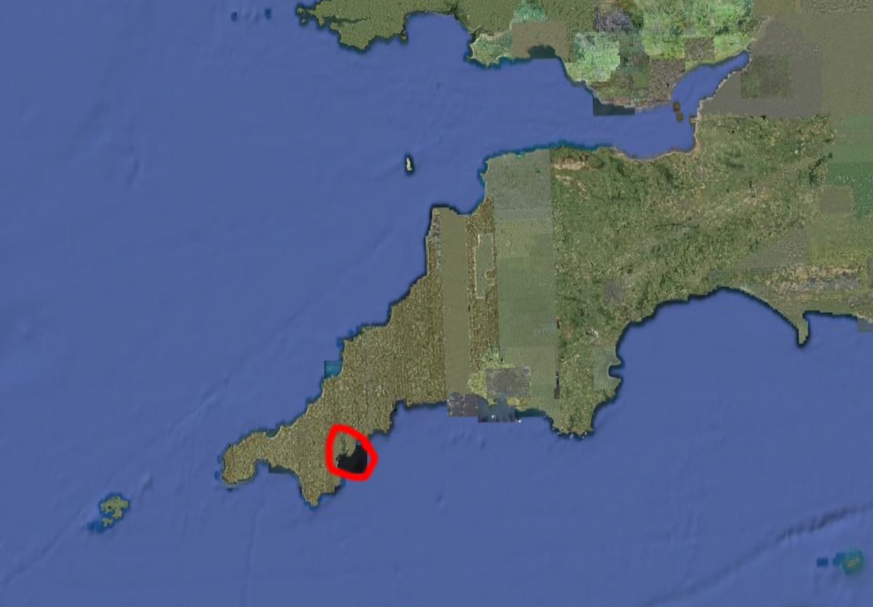
The Fal Estuary is located in Cornwall, South West England (Fig. 0.1). The estuary is a Ria, formed as a result of marine transgression during the Flandrian period between 8 and 3KaBP. The river Fal, along with 5 other main rivers, drains into the Carrick Roads waterway. The bathymetry of the ria reflects the topography of the original river valley, with a deep main channel of 30m and shallower side banks. Salt water dominates the estuary due to relatively low riverine inputs, therefore habitats in the estuary are predominantly marine. Relatively increased sedimentation occurs at the riverine end of the estuary, compared with the seaward end. This is represented by higher turbidity in the riverine end, which reflects on increased sediment load, resulting in sheltered mudflats where the water loses energy and releases the sediment from suspension. With a Spring tidal range of 5.3m around Falmouth, the estuary is macrotidal, becoming mesotidal in the upper reaches near Truro, with a 3.5m range. The Fal is the 3rd largest natural harbour in the world, but commercial development has been limited due to restricted infrastructure provision in the immediate area. In October 1996, the Fal estuary, covering 6387. 8 hectares, was designated a Special Area of Conservation (SAC) and Site of Special Scientific Interest (SSSI) by The Joint Nature Conservation Council and Natural England. This was due to the presence of sensitive biotopes such as Maerl and Eelgrass beds in the subtidal sandbanks (Langston et al. 2003) Maerl beds, composed of free living corallinaceae, act as a nursery ground for juvenile fish, including the rare Couch’s goby (Gobius couchi). Eelgrass (Zostera marina), is a particularly important habitat for maturing cuttlefish, seahorses and pipefish. Until the mid 1990s, the area around the estuary was extensively mined for the heavy metals copper, zinc and tin. Mine drainage lead to high levels of heavy metals polluting the water, especially around Restronguet Creek. In 1992, the Carnon River suffered an uncontrolled release of acidic heavy metal polluted water from the Wheal Jane mine due to the overtopping of the drainage system. Currently, only copper is present at elevated levels. The area is also designated as a sensitive area (eutrophic) by the Nitrates Directive 91/676/EC (Langston et al., 2003) The Fal estuary represents an area of complex biological, chemical and physical features, creating an area of immense oceanographic and biological interest.
|
||||||||||
| Introduction to the Fieldcourse |
|||||||||||
| For a two week period between 30th June to 9th July 2009, a multidisciplinary study of a variety of oceanographic and biological parameters in the Fal estuary was undertaken. In order to investigate the biological, chemical and physical characteristics of the region, three survey programs were undertaken covering the estuarine and offshore areas of study.
|
|||||||||||
| Abstract |
|||||||||||
|
The 2009 Falmouth field course consisted of three main parts. The first of these was a geophysical survey of a small segment of the Fal estuary. The main aim of this survey was to create a benthic map of the area and identify important habitats, several areas of interest were found, including a seagrass bed and a zone of sediment dominated by dead Maerl. The second part of the field course was an investigation into the biological and chemical parameters of the estuarine environment. This investigation provided results close to what would have been expected from a tidally dominated estuary, with well mixed water and decreasing nutrient concentrations downstream. The final part of the field course was an offshore investigation of water column structure. The principal aim of this part of the course was to determine the level of stratification in the water column, this was found to be relatively high. The secondary aim was to locate a front, this was not achieved.
|
|||||||||||
| Boats |
|||||||||||
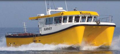
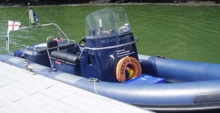
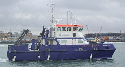
| In order to sample the three areas of study the following vessels were used as platforms
|
|||||||||||
|
|||||||||||
|
|
|||||||||||
| Equipment |
|||||||||||
| In order to sample the sites and obtain data the following equipment was used. The limitations of the equipment and assumptions also follow below each example. |
|||||||||||
|
|
|||||||||||
| Geophysical |
|||||||||||
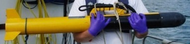
| Side Scan Sonar (SSS) (fig. 1.4)
|
Fig 1.4 A Side Scan Sonar Towfish |
||||||||||
| |
|||||||||||
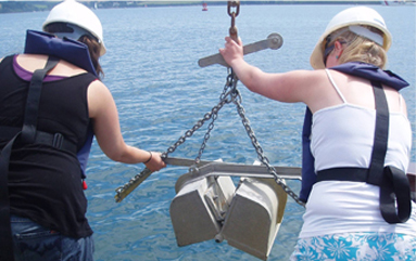
| Van Veen Grab (fig. 1.5)
|
Fig 1.5 A Van Veen Grab |
||||||||||
| |
|||||||||||
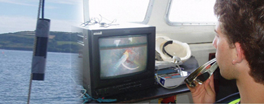
| CCD Video Camera and Monitor (fig. 1.6)
|
Fig 1.6 A CCD Video Camera and Monitor |
||||||||||
| |
|||||||||||
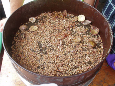
| Sieve stack (fig. 1.7)
|
Fig 1.7 A Sediment Sieve
|
||||||||||
| |
|||||||||||
| Estuarine |
|||||||||||
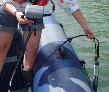
| YSI Probe (fig. 1.8)
|
Fig 1.8 A YSI probe
|
||||||||||
| |
|||||||||||
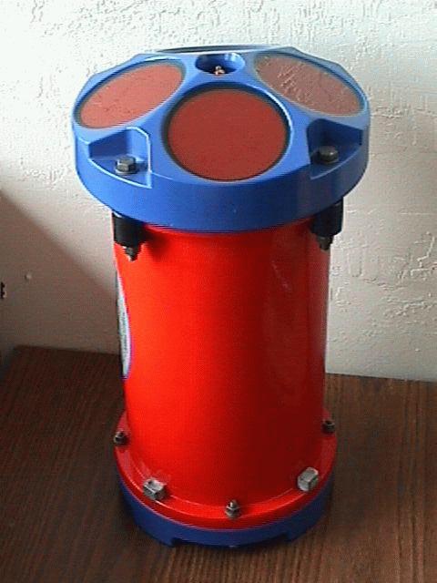
| Niskin bottles (fig. 1.9)
|
Fig 1.9 A Niskin Bottle Reference: http://courses.washington.edu/uwtoce06/webg2/methods/niskin.jpg
|
||||||||||
| |
|||||||||||
|
|
|||||||||||
| Offshore |
|||||||||||
| Acoustic Doppler Current Profiler (fig. 1.10)
|
Fig 1.10 An Acoustic Doppler Current Profiler Reference: http://www.oc.nps.edu/~stanton/miso/adcp.jpg
|
||||||||||
| |
|||||||||||
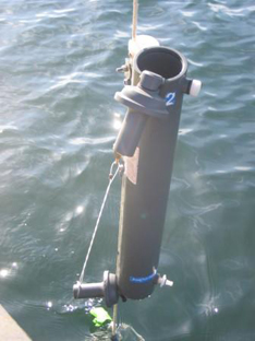
| Secchi disk (fig. 1.11)
|
Fig 1.11 A Secchi Disk
|
||||||||||
| |
|||||||||||
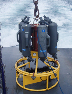
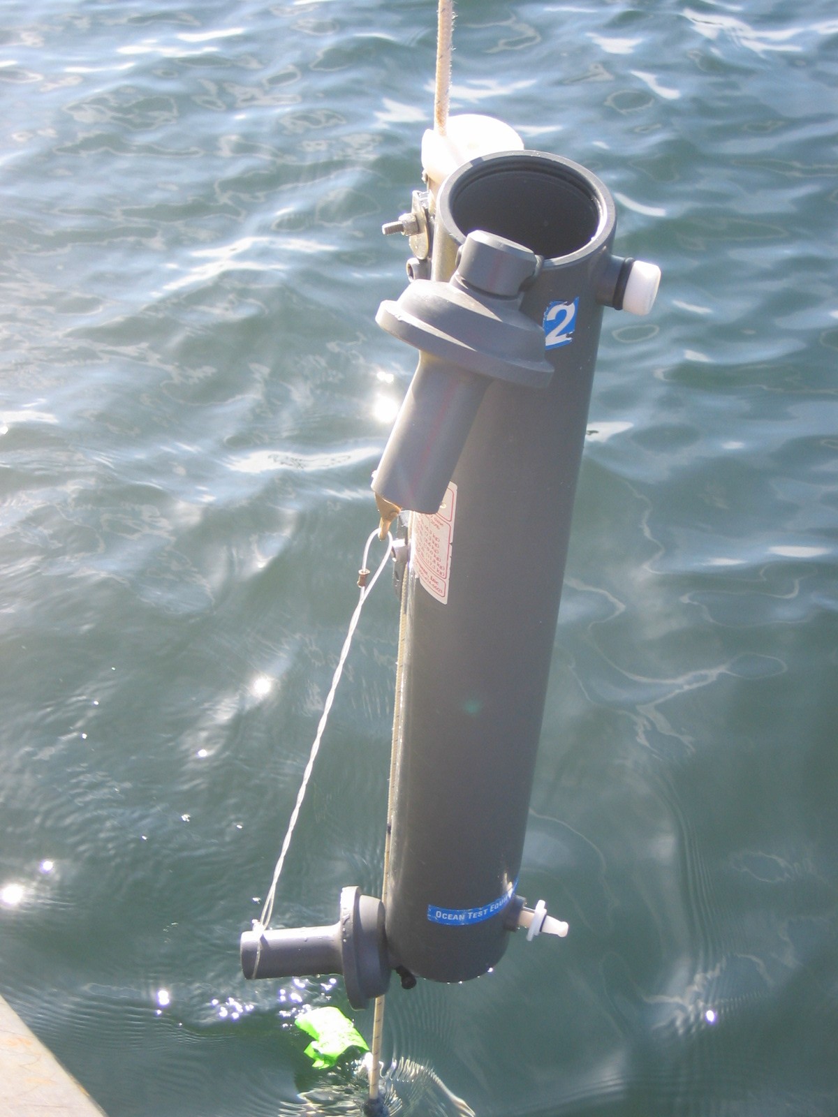
| CTD and Rosette (fig. 1.12)
|
Fig 1.12 A CTD and Rosette
|
||||||||||
| |
|||||||||||
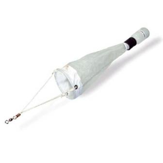
| Zooplankton Net (fig. 1.13)
|
Fig 1.13 A Closing Zooplankton Net Reference: http://www.envcoglobal.com/files/MO-WLD-426-AXX-L.jpg |
||||||||||
| |
|||||||||||
|
|
|||||||||||
| Aim |
|||||||||||
| The aim of the investigation was to produce a benthic habitat survey map of the Fal estuary due to specific interest from natural England to gather data for a nationwide biotope map.
|
|||||||||||
| Introduction |
|||||||||||
| The area studied is particularly interesting due to the maerl and seagrass beds. Maerl is of particular interest due to its recent economic exploitation and subsequent recovery. Seagrass is an important habitat for endangered species such the common seahorse and as an important nursery for juvenile fish. Both the seagrass and the common seahorse are vulnerable to stress from anthropogenic sources and non-anthropogenic habitat changes.
Date: 30/06/2009 AM- all times below in GMT
Location: Fal Estuary, Cornwall Sea state: Calm Wind: F2 Cloud cover: 1 Okta Vessel: MV Xplorer High tide: 11.16 GMT, 4.5m Staff: John Davis and Crew of the MV Xplorer
|
|||||||||||
|
|
Methods |
|
|||||||||
|
|
A subsurface Geoacoustics Dual frequency Analogue Side Scan Sonar tow fish operated at 100KHz, with a sweep time of 96ms and a swath width of 72m was used. Four transects were taken, though transects 2 and 3 were broken by a moored boat. The layback on the tow fish was negligible (3.8m) and the tow fish was 3m below the GPS receiver. Alongside this equipment a Van Veen grab with a bite size of 0.5m3 was used at 3 sites of particular interest. These sites were of specific scientific interest because they represented the most variation in habitats in the area sampled. This was shown by a video survey of these sites carried out before taking the grab. The video survey was also used to ensure that protected seagrass habitats were not damaged and that rock was not captured.
|
|
|||||||||
|
|
Survey Location |
|
|||||||||
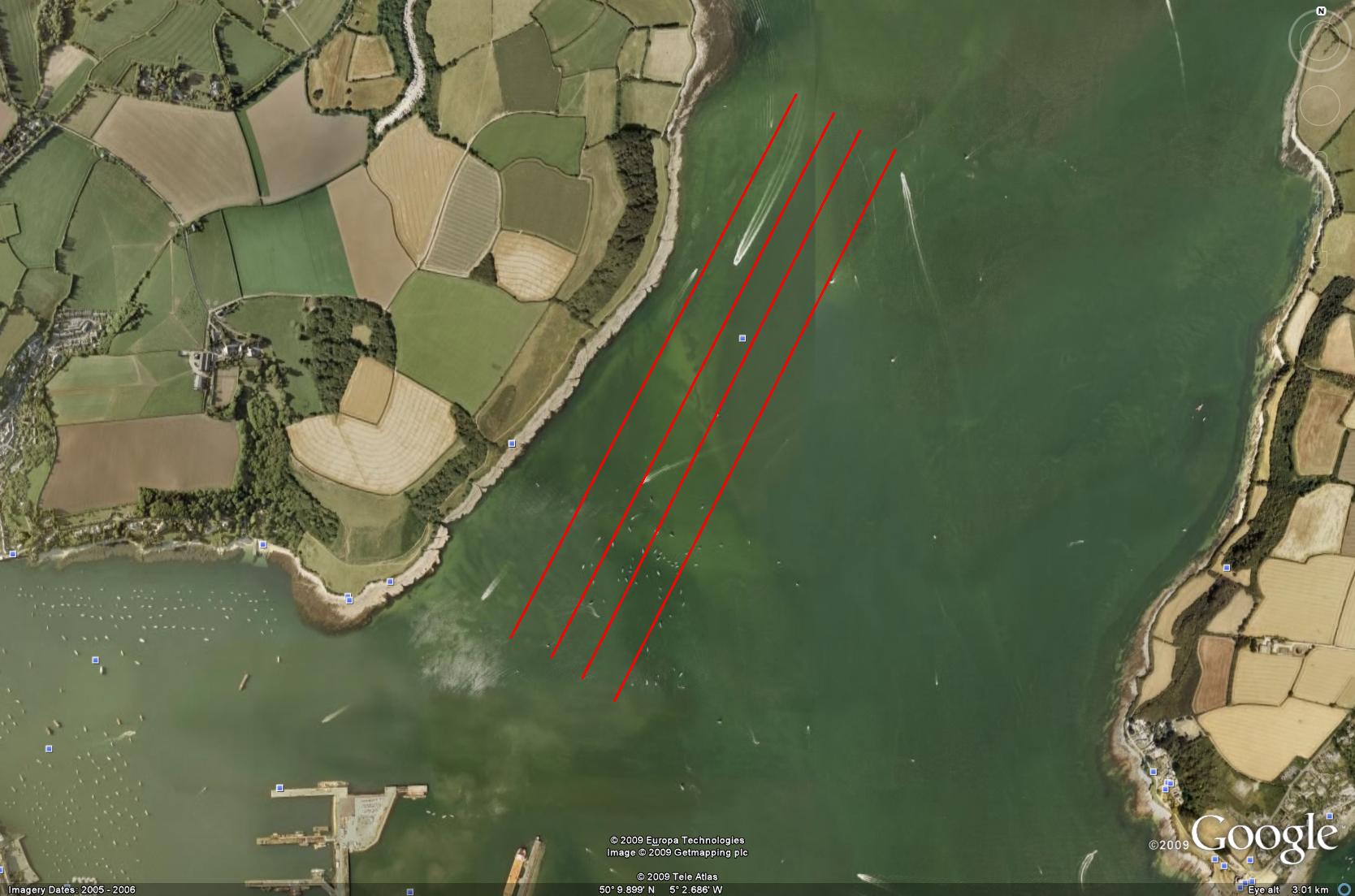
| The side scan sonar was carried out on the Western side of the Fal estuary close to the mouth of the Penryn river. As shown in Fig. 2.1.
Fig 2.1 A Location map of the Fal estuary and the adjoining rivers.
NB. Survey trace map shows a Google Earth image including the coordinate lines of our SSS tracks.
|
|||||||||||
| Site Background |
|||||||||||
| Langston et al. (2003) and The Fal and Helford Marine Special Area of Conservation Management Scheme (2008) suggests the area studied would be expected to show evidence of Maerl, the calcareous seaweed, and eelgrass (Zostera marina) in the subtidal sandbanks habitat. The presence of these unusual species is a primary reason for it’s designation as a Special Area of Conservation. Maerl, a coralline algae, is similar in appearance to encrusting algae, growing in the sub- littoral zone. It is pink in colour and grows in loose beds of fragmented nodules, as shown figure 2.6. |
|||||||||||
| Side Scan Sonograph |
|||||||||||
|
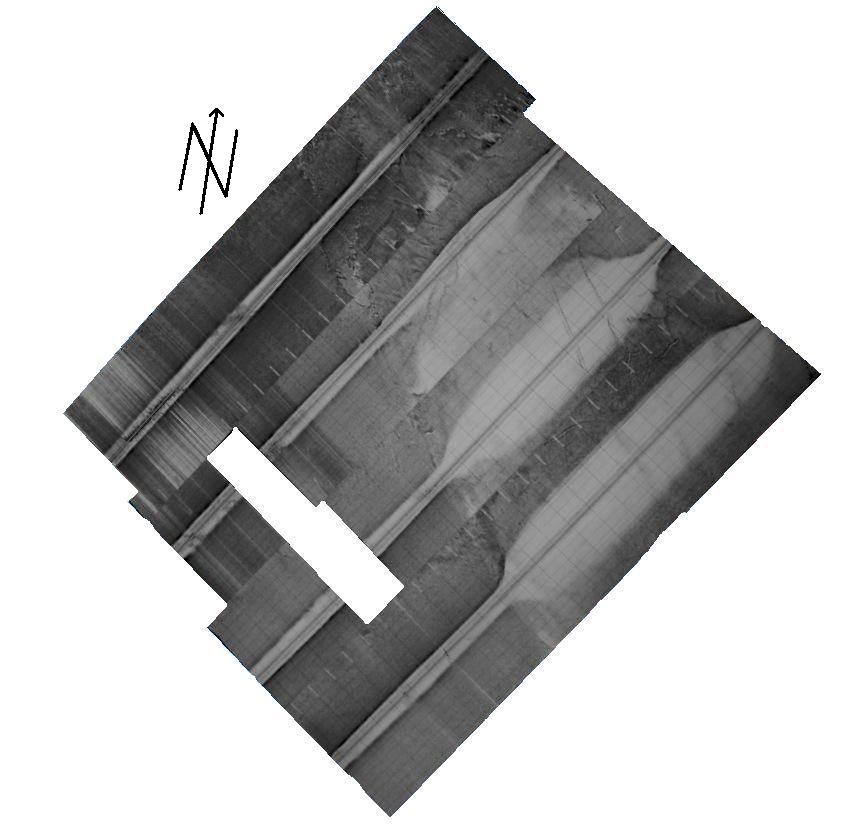
Fig 2.2 A photograph of the compiled backscatter print out from the SSS
|
Figure 2.2 is the Side scan sonar output showing variation in backscatter. These areas are then to translated to compose the benthic habitat map in fig 2.3. The white area inside the plot was an area not surveyed due to a Stationary boat.
|
||||||||||
| Side Scan Sonar Interpretation |
|||||||||||
|
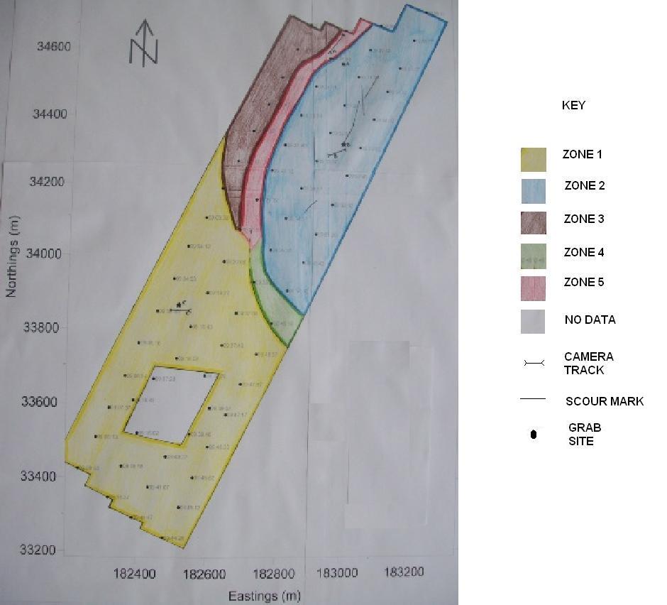
Fig 2.3 A Benthic Habitat map produced from the SSS
|
A track plot was created using Surfer 8 using the data from the GPS track log. The side scan sonar plot was used to calculate the wavelengths and heights bedforms. Benthic sediment zones were then identified using ground truthing information from the grabs this information was then translated onto the Benthic Habitat map (fig. 2.3) which shows distinct areas of habitat.
|
||||||||||
| Side Scan Sonar Overview |
|||||||||||
| There are five distinct benthic zones in the area surveyed. The largest of these (Zone 1) is in the south of the survey area, the predominant bedform being ripples of approximately 1m in wavelength. The clear area in the middle of the zone was caused by having to divert the course of the survey vessel due to the presence of a large moored yacht. The second largest zone (Zone 2) is the channel of around 30m depth, in the north east of the survey. Here the grab sample (Grab B) showed a fine sediment, as compared to a known example of the sediment comparison charts. The dominant bedforms in this area are scour marks, which are most likely to be caused by anchor drags. The scours have a range of sizes between 2.5 to 5 m in width and 0.5 to 1.0 m in depth. The third largest zone (Zone 3), in the north west of the area surveyed appears to be a rocky outcrop around 10-20cm high. No grab was taken here. Zones 4 and 5 are both in the area of transition between the deep channel (around 30 m) and the shallower areas (around 3 m in depth). Zone 4 is easily distinguishable on the sidescan output due to the obvious change in the water column depth. Inspection of the charts shows that there is 20-25m increase in depth over 50m. The boundaries of this zone can be treated as a proxy for bathymetric contours. Zone 5 is less easily distinguished on the sidescan output, the boundaries being the edges of zones 2 and 3.
|
|||||||||||
| Grab A |
|||||||||||
|
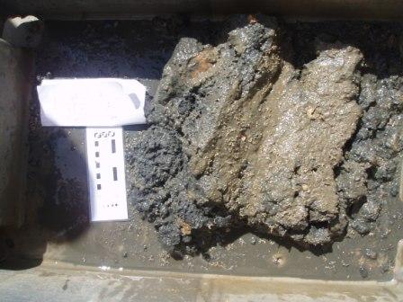
Fig 2.4 A photograph of Grab A showing the sediment found in the Van Veen grab |
Location: 50° 10.2876N 05° 02.4167W Time: 10:34 GMT Depth: 18.5 metres The video footage appeared to show sandy sediment with both green and red macroalgae growing. This video also contained seagrass so the grab site was moved before the grab was obtained, as seagrass is a protected biotope. This grab sample (Fig 2.4) was made up of fine muddy sand with an oxic layer of around 2cm in depth. There was a small amount of dead Maerl (less than 5% coverage) found on top of the sediment. Also found: terebellid polychaetes, bivalve molluscs and nematodes.
|
|
|||||||||
|
|
Grab B |
|
|||||||||
|
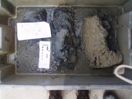
Fig 2.5 A photograph of Grab B showing the sediment found in the Van Veen grab |
Location: 50° 10.1583N 05° 02.4162W Time: 11:24 GMT Depth: 32 metres The video footage appeared to show possible sandy sediment with a bare seafloor. The grab (Figure 2.5) sampled fine, cohesive sandy mud with an oxic layer of around 3cm depth. Polychaetes and nematodes were abundant throughout the sample. No Maerl was found at this site. |
||||||||||
| Grab C |
|||||||||||
|
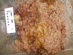
Fig 2.6 A photograph of Grab C showing the sediment found in the Van Veen grab
|
Location: 50°09.8930N 05°02.7830W Time: 11.52 GMT Depth: 9.3 metres The video footage appeared to show possible coarse sandy looking sediment with some shells and algae present. The grab sample (Figure 2.6 ) was predominantly Maerl, around 30% of which was alive. Also found: bivalves, a small (<1cm total width) hermit crab, bryozoans, an amphipod, dead macroalgae and gastropod molluscs attached to shells and other hard substrates.
|
||||||||||
|
|
|||||||||||
| Aim |
|||||||||||
| To obtain an understanding of, and investigate the interactions between, the biological, chemical and physical processes occurring within the Fal estuary.
|
|||||||||||
| Introduction |
|||||||||||
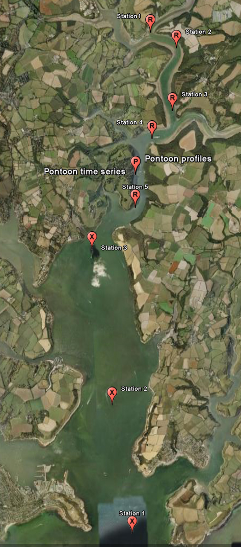
| In order to assess the distribution of nutrients within the estuary, a number of variables were studied; temperature, salinity, oxygen saturation, and nutrient concentration, at equal depth intervals at several locations. The vessels Ocean Adventure RIB and MV Xplorer along with the King Harry Ferry Pontoon (lat: 50º 30.050, long: 05º 02.300) were used as sampling platforms to obtain data from Black Rock at the mouth of the estuary to Malpas, 6 nautical miles upstream. Half the group were located on the pontoon while the rest travelled up the estuary on the Ocean Adventure RIB. The MV Xplorer was then used to take deep water from the seaward end of the estuary. The investigation was carried out on 03.07.09
|
|||||||||||
| Method |
|||||||||||
| Ocean Adventure RIB The Ocean Adventure RIB was used to sample further upstream to support the pontoon data and explorer to provide a detailed data range. From this vessel water samples were collected at four Stations from the surface and at 3m depth. The oxygen samples were processed in situ, using the Winkler method (Grasshoff et al 1999) and were later analysed in the lab for nitrate, phosphate, silicate, phytoplankton, chlorophyll and dissolved oxygen.
King Harry Ferry Pontoon The King Harry Ferry Pontoon was used as a sampling platform to obtain a time series of data throughout the tidal cycle. A YSI probe was deployed from the pontoon every half hour, measuring depth, temperature, pH, salinity, and percentage saturation of oxygen. Data was recorded every 0.5m down to a maximum of 6 metres at high water. Additionally, every hour water samples were collected from the surface waters and at maximum available depth. The oxygen samples were processed on site as per above with the Winkler method (Grasshoff et al 1999) to later be analysed in the lab for nitrate, phosphate, silicate, phytoplankton, chlorophyll and dissolved oxygen.
MV Xplorer Three sites in the lower reaches of the Fal estuary were sampled using the MV Xplorer. At each site a CTD rosette with 6 Niskin bottles attached was deployed. An initial profile of the water column was analysed in order to determine the depths of the three water samples to be collected. These depths reflected interesting features or gradients within the water column to be investigated such as the location of the thermocline. The samples were processed onboard for nitrate, silicate, phosphate, phytoplankton and dissolved oxygen to be later analysed in the lab. In addition to this, horizontal zooplankton trawls were carried out using a 200µm zooplankton net, formalin was added to samples to preserve the organisms for later analysis. The secchi disk was also used to determine the light penetration depth at each site. The light penetration depth is essential for locating the likely areas that phytoplankton will occur because phytoplankton require light to photosynthesise and are unlikely to occur under this depth during the day .
|
|||||||||||
| Results and Discussion |
|||||||||||
|
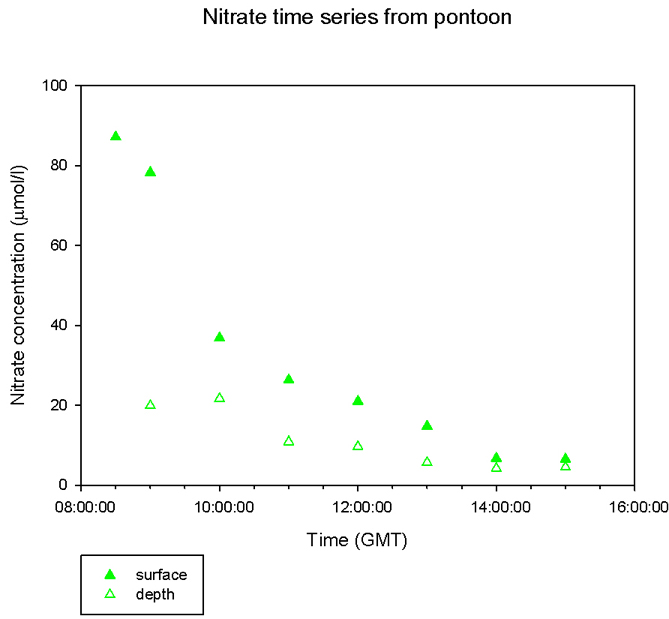
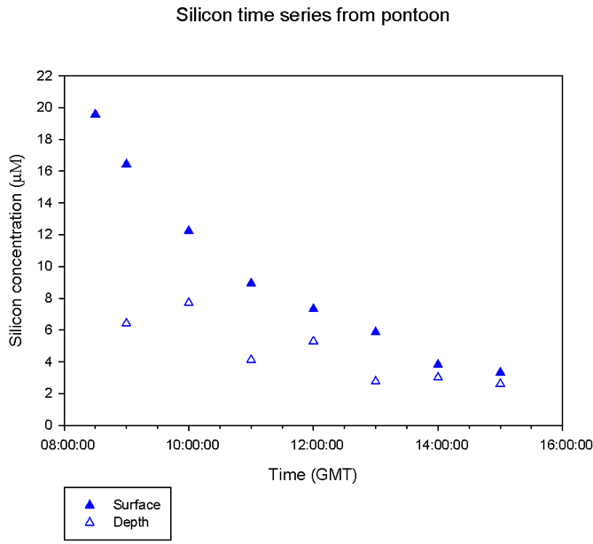
Fig 3.1 Nitrate concentration over time in the Fal Estuary
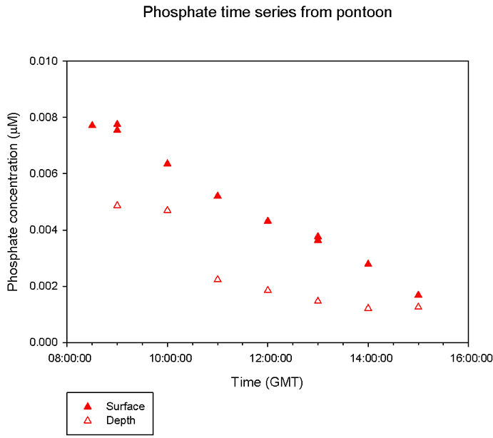
Fig 3.2 Phosphate concentration over time in the Fal Estuary
Fig 3.3 Silicate concentration over time in the Fal Estuary
|
Water sampling in series on the Pontoon The graphs fig 3.1, 3.2 and 3.3 show a time series analysis of Nitrate, Phosphate and Silicate concentrations respectively.
Surface water samples The highest nitrate concentration at the surface is 87.2µM recorded at 08.30GMT just after low tide (which occurred at 08:17GMT). The highest phosphate concentration (1.13µM) and highest silicate concentration (19.57µM) were also recorded at this time. Freshwater contains the highest concentration of these substances, concentrating them from the land in the drainage basin and transporting them to the river. Therefore, the higher the proportion of freshwater present, the higher the concentration of nitrate, phosphate and silicate. The high concentration of these nutrients in the freshwater may be due to the high levels of precipitation the previous day, causing a large increase in the volume of ground water and run-off entering the river. The lowest nitrate concentration at the surface is 6.5µM and it was recorded at 15.00GMT shortly after high tide at 14.10GMT. The lowest phosphate concentration (0.45µM) was recorded at 14.00GMT and lowest silicate concentration 3.32µM was found at 15.00GMT. The low concentrations found at this time is due to an increased proportion of seawater in the estuary at high tide
Deep water samples The highest nitrate concentrations at depth were 19.9µM and 21.7µM recorded at 9:00 and 10.00GMT respectively, just after low tide at 08:17GMT. The highest phosphate concentration (0.74µM) and highest silicate concentration (7.71µM) were also recorded at these times. The lowest nitrate concentration at depth is 2.61µM and it was recorded at 15:00GMT shortly after high tide at 14:10GMT. The lowest phosphate concentration (0.23µM) and lowest silicate concentration (2.61µM) were also found at this time. Concentrations are lower at depth as this is where the denser saline water is present, which contains less nutrients. Fresh water containing higher levels of nutrients is less dense and flows in the upper surface layer.
|
||||||||||
|
|
|||||||||||
| Water Sampling for Stations on the Ocean Adventure and Xplorer | |||||||||||
|
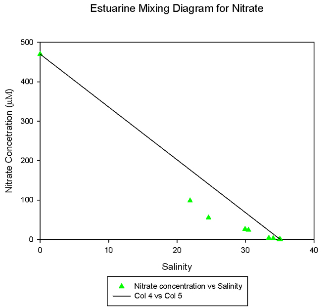
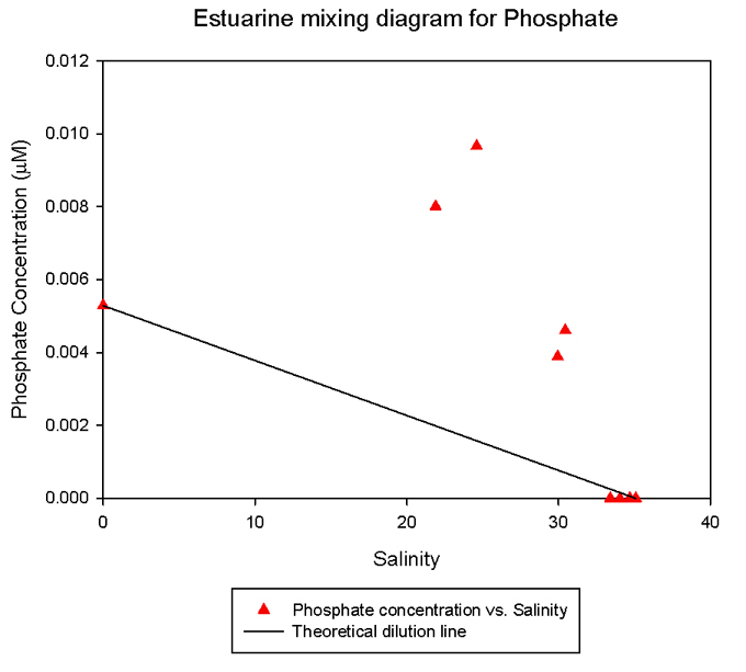
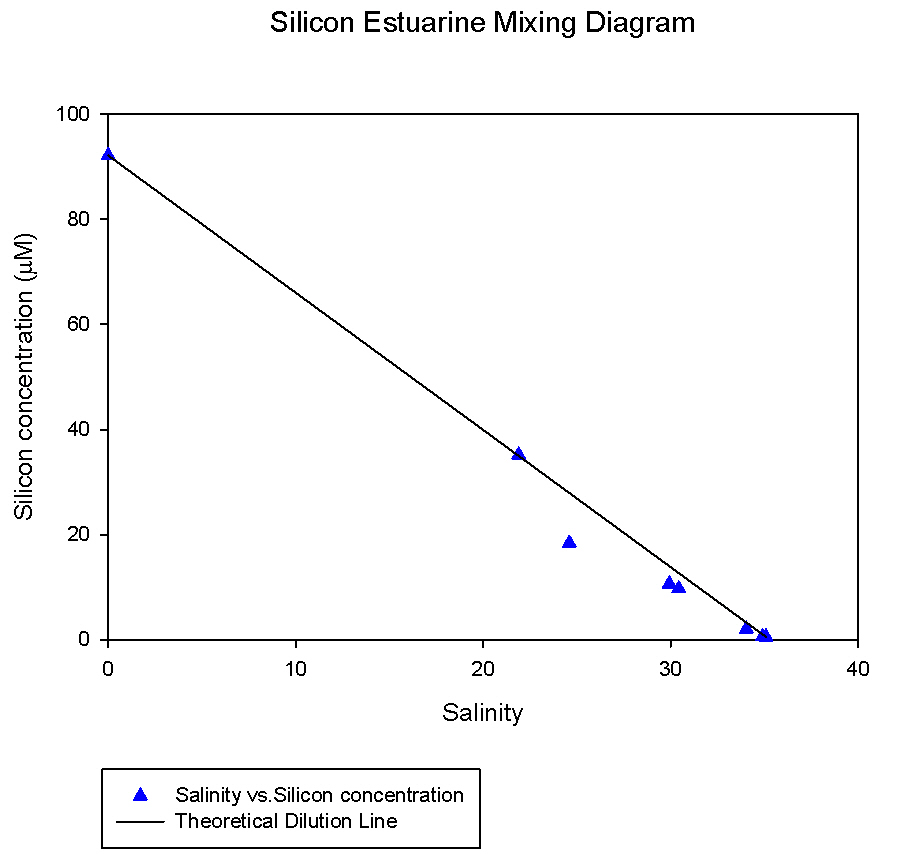
Fig 3.4 An Estuarine Mixing Diagram for Nitrate in the Fal Estuary
Fig 3.5 An Estuarine Mixing Diagram for Phosphate in the Fal Estuary
Fig 3.6 An Estuarine Mixing Diagram for Silicate in the Fal Estuary
|
Nitrate, Phosphate and Silicon have each been analysed and an estuarine mixing diagram has been created in order to find the behaviour for each nutrient. This is done using a theoretical dilution line (TDL) which has the following assumptions.
Nitrate Figure 3.4 shows an estuarine mixing diagram for the Fal Estuary, plotting nitrate against a conservative seawater constituent, salinity. The riverine end member collected from Truro had a salinity of 0 and a nitrate concentration of 470μM. The marine end member, collected from Black Rock (50° 8.572 N 5° 01.718 W) had a salinity of 35.09 and a nitrate concentration of 0.2 μM. Dilution of nitrate occurs with the transition into more saline waters, away from the main nitrate source which is the two sewage works upriver from Malpas, although tributaries joining the main channel may act as additional smaller sources of the nutrient. Nitrate appears to be behaving non-conservatively throughout the estuary with removal from the system. This may be due to phytoplankton removing nitrate from the system for processes such as protein production and cell growth.
Phosphate Figure3.5 shows an estuarine mixing diagram for phosphate concentration against a conservative sea water constituent, salinity. The riverine end member, collected at Truro, had a phosphate concentration of 0.005µMol. The marine end member from Black Rock (50° 8.572 N 5° 01.718 W), with a salinity of 35.09, had a phosphate concentration of 0.000 µMol. N.B Most alues were below detectable limits
Samples taken at lower salinities fall above the theoretical dilution line (TDL).This is non-conservative behaviour with phosphate being added to the system. TDLs are based on the assumption that there is only one source of phosphate to the river. This assumption is not upheld with this TDL as the Tresillian River, Calenick Creek and Lambe Creek all joining the main Truro River defy the assumption that there are no secondary riverine inputs into the estuary. The Tresillian River joins the main channel at the least saline sampling point (Station 1 at Malpas: 50° 14.708 N 5° 01.376 W). Upstream of this confluence, on the Truro River, is a sewage works at 50 14.900 N 5 02.600 W. The Tresillian River also has a sewage works at 50 16.540 N 5 0.460 W. These sites are very likely to be adding high quantities of phosphate to the system, and so may explain why the phosphate concentration is higher than the TDL prediction.
Silicate Fig 3.6 is the estuarine mixing diagram for dissolved silicon in the Fal Estuary, plotting silicate concentration against a conservative seawater constituent, salinity. The riverine end member collected from Truro had a salinity of 0 and a silicate concentration of 92.1μM. The marine end member, collected from Black Rock (50° 8.572 N 5° 01.718 W) had a salinity of 35.09 and a silicate concentration of 0.5 μM. Silicate appears to be behaving non-conservatively, as there is removal of silicate between salinities of 22 and 24.6, by up to approximately 10μM below the expected value. This may be due to a bloom of diatoms in the estuary removing silicate from the system for growth of the silicon-based frustule. This assumption cannot be confirmed, as no phytoplankton sample was taken at Station 2, in the middle reaches of the river, where the main silicate removal appears to occur. However, high numbers of diatoms were found at other sites in the estuary, for example Station 4, which may support this assumption.
|
||||||||||
|
|
|||||||||||
|
|
YSI Analysis |
|
|||||||||
|
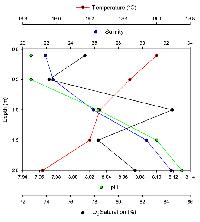
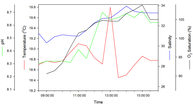
Fig 3.7 Temperature, Salinity, pH and Oxygen changes with Depth at Station 1 on the Ocean Adventure
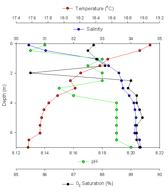
Fig 3.8 Temperature, Salinity, pH and Oxygen changes with Depth at Station 2 on the Ocean Adventure
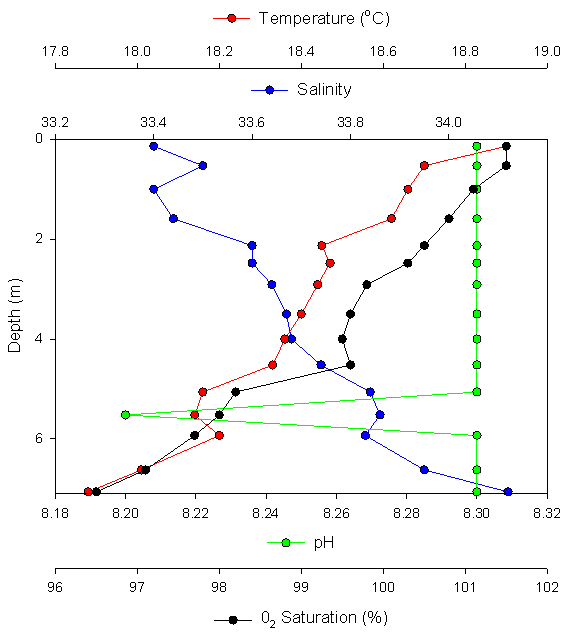
Fig 3.9 Temperature, Salinity, pH and Oxygen changes with Depth at Station 5 on the Ocean Adventure
|
Ribs Temperature The variation in temperature with depth appears to increase downstream: at Station 1, the furthest upstream at Malpas, (Fig. 3.7-3.9) temperature values vary by 0.7 ºC (19.6 ºC – 18.9 ºC) over a depth of 2m. At Station 2, there is a variation of 1.7 ºC over 7m depth (fig 3.8). This variation is most likely due to the increasing depth of the measured water column downstream, as the channel deepens, colder water is found at depth. Surface temperature is warmest at Station 1.
Salinity The greatest variation in salinity was observed highest up the estuary at Station 1 (fig 3.7), from 22 – 33 over 2m depth. This is as expected, as it is the point closest to the freshwater input, a particularly important factor given the heavy rainfall in the 24 hours previous to sampling. On progression downstream salinity becomes more uniform throughout the water column, as would be expected in a tidally dominated and therefore well mixed estuary. At Station 5 (fig 3.9), the furthest downstream salinity is 33.4 at the surface and 34.1 at the estuary floor, 6.5m down. Just over 6% of the variation found at Station 1.
pH Overall, pH observed remained around an average value of 8.1. With the exception of Station 1 (fig 3.7), pH varies by 0.1 over the depth of each Station. At Station 1 (fig 3.7), a variation of 0.2 was observed. In most cases pH variation correlates well with salinity. In areas where this is not the case the most likely cause is run off from the surrounding area.
Oxygen On progression downstream, oxygen saturation increases, from (surface) values of 76.0% at Station 1(up the estuary) to 101.5% at Station 5 (nearer the mouth of the estuary). Surface values in particular may be affected by the degree of wind mixing at the time of sampling, as stronger winds will act to increase the amount of air and therefore oxygen, mixed into the surface waters. At depth, oxygen saturation is also seen to increase, from 82.0% at Station 1 to 96.0% at Station 5. Within the profiles at each Station, some degree of variation was observed: Stations 1, 2 and 3 show an increase of less than 6% in oxygen saturation down the depth profile, whereas Stations 4 and 5 show decreases of 1% and 5% respectively. This may be due to phytoplankton excretion of oxygen and atmospheric interactions in the mixing. The decreased values upstream may be due to increased biological oxygen demand (BOD), especially as effluent from the two sewage works, as identified in the nitrate analysis, may be present in the water column. Increased values at depth may represent the increased turbulence from the tidal waters, on the flooding tide, which will encourage mixing within the water body. Also, photosynthesising phytoplankton add to the oxygen content of the water body. An increased oxygen saturation value may therefore be indicative of phytoplankton, although this is an assumed correlation. |
|
|||||||||
|
|
|||||||||||
| Pontoon | |||||||||||
|
|
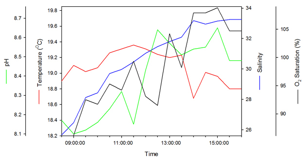
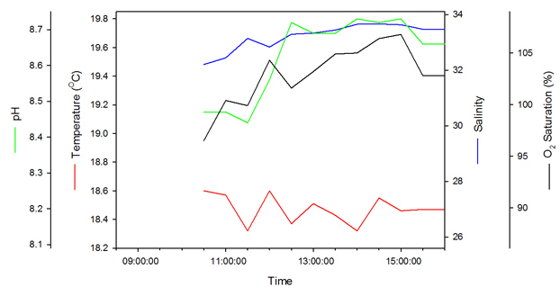
Temperature Temperature measured from 0830 GMT until 1530 GMT at the surface increased by 0.5 ºC, over the time period. This is likely to be due to increasing solar irradiance throughout the day (figs 3.10-3.12). From 1200 onwards, the water column at depth also increases in temperature, probably due to the flooding tide bringing warmer water up the estuary. At 1430, just after high tide, a maximum temperature of 18.2 ºC was observed at 5.5m depth.
Salinity The pattern of salinity at the pontoon (figs 3.10-3.12) reflects the data from the RIB. The greatest variation was found in the first YSI profile taken first, at 0830 GMT, in this profile the salinity varied from 22.6 at the surface to 31.3 at the bottom (1.5m), a change of 8.7. This was at low tide, when there would be a relatively greater proportion of freshwater than at high tide. The profile taken closest to high tide (14.00GMT) shows a salinity variation of 0.7 over a depth of 6m, reflecting the higher proportion of seawater present.
pH The pontoon data shows an increase in pH over the time series. The first reading, at 08.30GMT, shows a pH of between 8.1 – 8.3 (fig 3.10), over 1.5m depth, increasing to a pH of between 8.6 – 8.7 at 15.00GMT (fig 3.11), over a depth of 5.5m. This may be due to the flooding tide up to high water at 14.10GMT, bringing in more saline waters with a higher pH. A trend of higher pH was also observed at shallower depths over the time series, as the tidal waters became more dominant, notably at 14.00GMT, where a pH of 8.7 is seen up to a depth of 2m. Overall, no more than 0.2 pH variation was observed over any given depth, suggesting that despite the increase in pH over the tidal cycle, there is little variation within the water column.
Oxygen Oxygen saturation increases with depth until 10.30GMT, where a spike of 2% is observed at 1.0-1.5m depth (fig 3.10-3.11). This is seen to develop at 1100GMT, an increase of 80% from 1.5- 2.5m. This may reflect increased mixing during the fastest part of the flooding tide. Following this, the percentage oxygen saturation is observed to then decrease with depth, as at 14.00GMT. This may reflect the low tidal currents around the turn of the tide, as less mixing takes place.
|
|
|||||||||
|
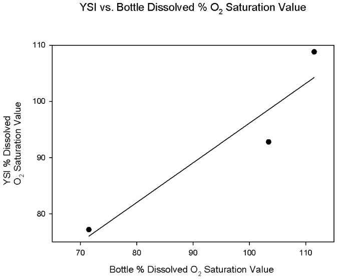
Fig
3.13 YSI vs bottled dissolved oxygen saturation in the
Fal Estuary
|
N.B. As shown by fig 3.13 (YSI vs. Bottled Oxygen), there is a good relationship between the percentage dissolved oxygen saturation values taken from the YSI probe and the measured values from the bottled samples, with an r2 value of 0.89. CTD measurements were taken on the Xplorer during the estuarine practical. However, the CTD was not calibrated for dissolved oxygen saturation. Therefore, values of, for example, 37.8 from the CTD are not correct or reliable. However, these values do indicate a pattern of increasing dissolved oxygen saturation with depth: for Station 1 at the surface, O2 is indicated by a value of a 35.5, at a depth of 6m registered a value of 38.2 and at 12m a value of 40.9. This does not reflect the pattern observed from the bottled dissolved oxygen saturation values of 108.1% at the surface, 110.2 at 7m and 105.8 at 12m. Therefore there is no correlation between the CTD and the bottled values for the Xplorer data and as such the CTD profiles should only be treated as guides to changing saturation within the water column and not an accurate representation of real values. |
|
|||||||||
|
|
Phytoplankton (figure 3.14) |
|
|||||||||
|
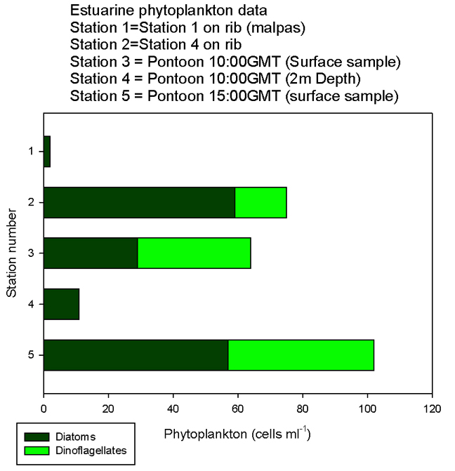
Fig 3.14 The number of phytoplankton cells of various groups at Stations 1-5 in the Fal Estuary
|
Station 1 – RIB (Malpas) There were very low numbers of phytoplankton found at this sampling site with diatoms making up 100% of species found. This may be because the water here has high turbidity, with lots of suspended particulate matter (SPM) from terrestrial sources. This inhibits phytoplankton growth by decreasing the depth of the euphotic zone. The water here is fast flowing, meaning that the water column has no stratification.
Station 4 – RIB In total there was a concentration of 75 cells/ml, this was dominated by diatom cells, with only ~20 % of cells in the sample being dinoflagellates. Station 4 was much further down stream, and therefore had lower levels of SPM and a less well mixed profile. These conditions are better suited for growth of phytoplankton, leading to the observed increase in numbers.
Pontoon - 10:00 GMT surface The total concentration of phytoplankton was 64 cells/ml, with the ratio of diatoms to dinoflagellates being roughly equal. This sample was taken just after low water, meaning that the surface waters had a relatively low salinity. Stratification between the fresher surface waters and more saline bottom waters is high at low water, with high solar irradiance at the surface. Phytoplankton become trapped in the surface waters leading to a high concentration being observed.
Pontoon – 10:00 GMT 2m No dinoflagellates were observed in this sample, with a total concentration of only 11 cells/ml being completely dominated by diatoms. The lower irradiance levels at depth favour the growth of diatoms, resulting in the concentrations observed.
Pontoon – 15:00 GMT surface The highest concentrations of 102 cells/ml were observed here, with the sample being taken just after high water. The ratio of diatoms to dinoflagellates was roughly equal, with 56% diatoms and the remaining 44% dinogflagellates. This may be because they may have been brought upstream with the flooding tide.
|
||||||||||
|
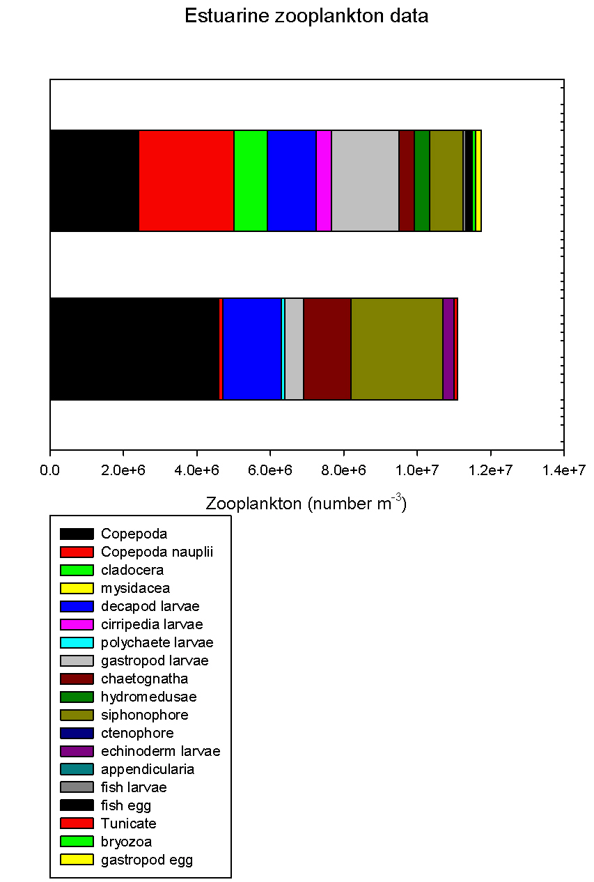
Fig 3.15 Species composition of zooplankton at Stations 4 and 5 in the Fal Estuary
|
Zooplankton (fig 3.15) Xplorer – Station 1 – Black Rock A value of 1.2x10⁷ zooplankton/m3 was recorded, with roughly 40% of this being made up of copepods. Around 20% was siphonophores, with the remainder being made up of copepod nauplii, decapod larvae, polychaete larvae, gastropod larvae, chaetognaths, echinoderm larvae and tunicates.
Xplorer – Station 3 – Feock A value of 1.1x10⁷ zooplankton/m3 was recorded, with roughly 20% copepods and 20% copepod nauplii. Roughly 15% was gastropod larvae and 10% decapod larvae, the remainder of the sample was made up of cladocera, cirripede larvae, chaetognaths, hydromedusae, siphonophores, fish larvae and eggs, bryozoan larvae and gastropod eggs. Station 1, located further offshore near to Black Rock, showed a slightly smaller number of zooplankton than Station 3. Station 3 showed a slightly different composition of zooplankton, also with a wider variety of species.
|
|
|||||||||
| Conclusion |
|||||||||||
| Our aim to obtain an understanding of the interactions between the biological, chemical and physical processes occurring within the Fal estuary was fully investigated. The highest nutrient concentrations were found at the riverine end member, and decreased towards the seaward end member, for example nitrate levels of 470μM decreased to 0.2μM. Higher nutrient concentrations in the lower density freshwater result in much higher nutrient concentrations being recorded at the surface compared to the lower nutrient concentrations in the higher density saltwater. Temperature is highest at the surface due to the incoming solar radiation heating the surface waters, this radiation decreases with depth as it is absorbed. Throughout the time series recorded from the pontoon temperature increased by on average 0.5ºC. Salinity increases with depth, with lower density fresh water overlying the higher density saltwater, with the greatest range being recorded at low water. Throughout the estuary pH remains relatively constant, however upon the flooding tide an increase in pH from 8.1 to 8.3 was recorded. Generally oxygen concentration increases downstream, also increasing with depth. Surface oxygen concentrations increase from 76.0% upstream (Station 1) to 101.5% downstream (Station 5), the values recorded at depth also increase but by a lesser degree. Phytoplankton numbers in the surface waters were highest around high water, and lowest around low water, while the lowest values were recorded at depth due to the highest irradiance and nutrient levels being found in the surface waters. Zooplankton levels at both Stations were relatively low with only slight variations in the composition and abundance of species present.
|
|||||||||||
|
|
|||||||||||
| Aim |
|||||||||||
| To carry out offshore surveying in order to determine the degree of stratification within the water column following high wind conditions and in addition, attempt to locate a frontal system, previously located in the area.
|
|||||||||||
| Introduction |
|||||||||||
|
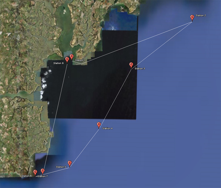
Offshore surveying was carried out on RV Callista on
7th June 2009, with six Stations being sampled along a transect
from Dodman Point to Black Head (fig. 3.1)The length and direction
of the transect was chosen in order to locate the frontal system following
a period of rough weather. Samples were also taken at Black Rock
as practice Stations.
Fig 3.1 Map of offshore Stations
|
|||||||||||
| Methods |
|||||||||||
| The CTD, attached to the Niskin bottle rosette, was deployed at each Station in order to measure conductivity (and therefore salinity), temperature, fluorescence and light at depth. This was done to locate the thermocline and peaks in chlorophyll, indicating the presence of phytoplankton. This real time data was used to determine the depths at which water samples were to be taken: samples were taken below, on, and above the thermocline to provide a representative sample of the water column. Phytoplankton were collected at the depth of the chlorophyll peak. Niskin bottles were fired at the required depths, and the apparatus recovered. The water samples were processed onboard for later analysis of oxygen saturation, nitrate, phosphate, silicate and phytoplankton. The ADCP measured the flow velocity at each Station. Zooplankton samples were taken from just below the depth of the chlorophyll peak, as they tend to graze on the phytoplankton from below. High levels of backscatter from the ADCP also indicated the presence of zooplankton. A closing net was deployed to vertically trawl to sample the zooplankton at the depth of highest backscatter. Formalin was added to the samples to preserve the zooplankton for microscopic analysis. The Secchi disk was deployed at each Station to measure the Secchi depth, which is a guide to the depth of the euphotic zone and light attenuation coefficient, supporting the CTD rosette data.
|
|||||||||||
| Results and Discussion |
|||||||||||
| CTD | |||||||||||
|
|
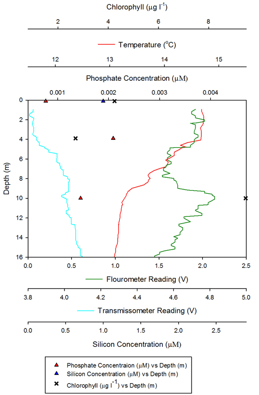
Station 1 Station 1, Black Rock at 08.17GMT (lat: 50º 08.323N, long: 05º 01.509), shows a highly stratified water column in terms of temperature. The thermocline occurs between depths of 4-8m, with a variation of 1.5° C observed between surface and lower water masses. Station 1 shows a defined peak in fluorometer readings, indicating increased chlorophyll presence, at a depth of 1m below the thermocline. The depth of peak fluorometer readings is echoed at Station 8, however the position of the peak is raised relative to the thermocline. There is also a higher chlorophyll value corresponding to a higher fluorometer reading at a depth of 10m. The phosphate values shown indicate an even mixing of the nutrient throughout the water column, as the values show little variation. However, there are only three values for phosphate, therefore no assumptions may be made regarding a trend.
|
||||||||||
| |
|||||||||||
|
|
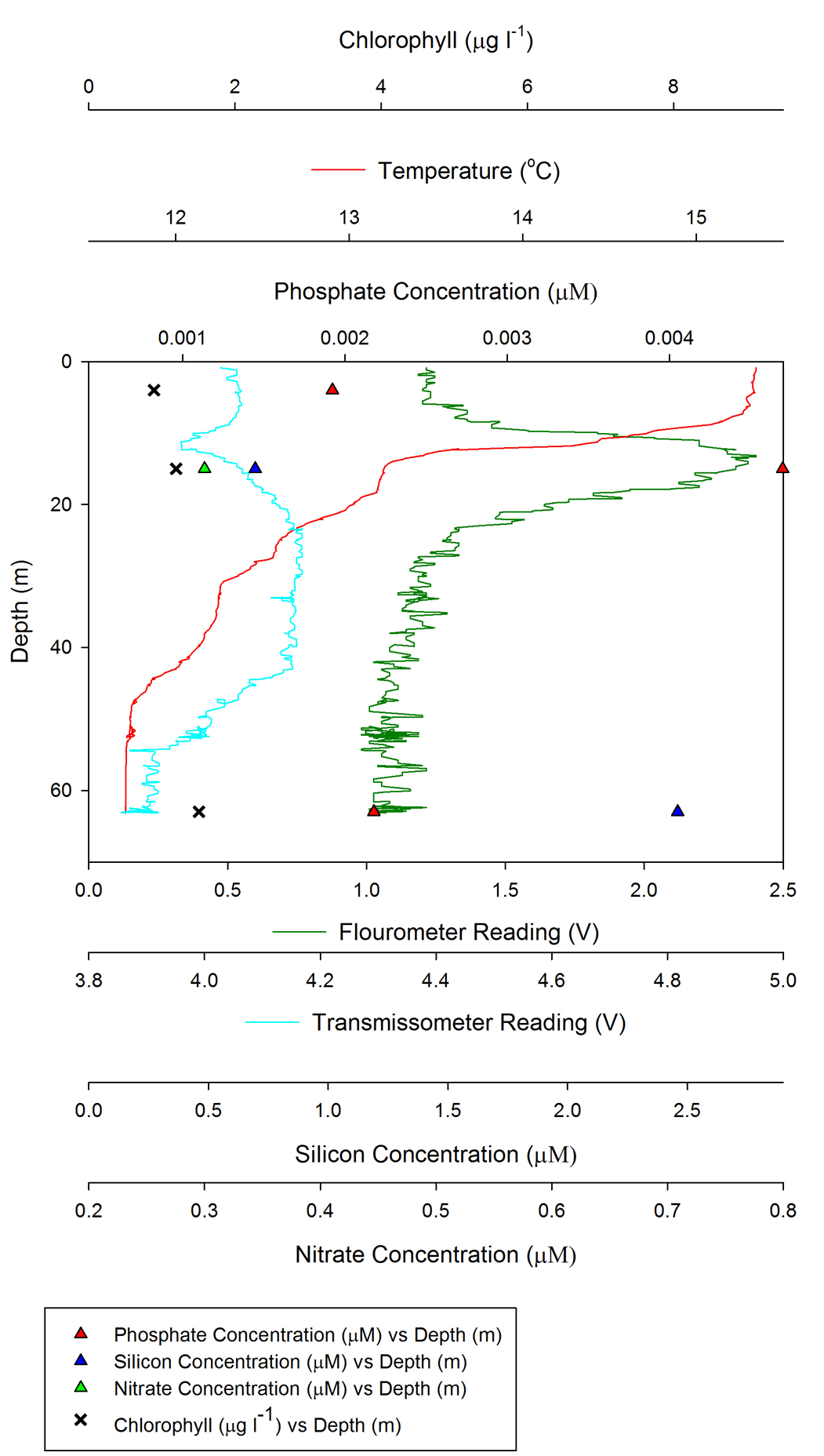
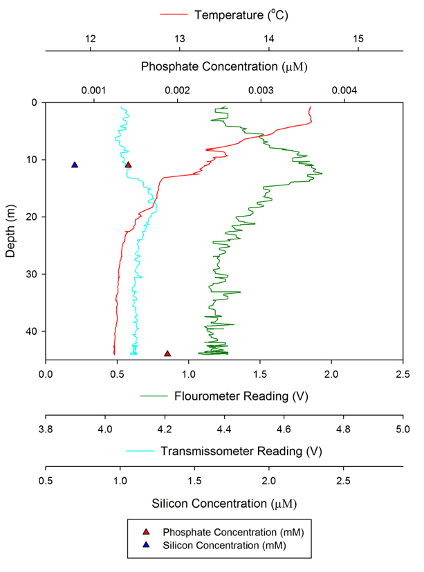
Station 5 Station 5 (lat: 50º 00.900, long: 05º 05.217) at 12.40GMT , furthest offshore, shows the most pronounced thermocline of all Stations, variation in temperature between surface and lower waters occurs over a shallow gradient (10-50m), in the order of 3°C. The peak fluorometer reading occurs at around 18m depth within the euphotic zone (calculated from Secchi depth) and in the region of most marked temperature change. Variation in silicon concentration indicates apparent uptake by biota in surface waters, whereas below the thermocline, levels are relatively higher due to the absence of such concentrations of biota. Chlorophyll values do not show any correspondence to the fluorometer readings. However, there is a higher value of phosphate seen at the fluorometer peak at 10m, which may suggest the presence of phytoplankton due to the increased nutrient level here.
|
||||||||||
|
|
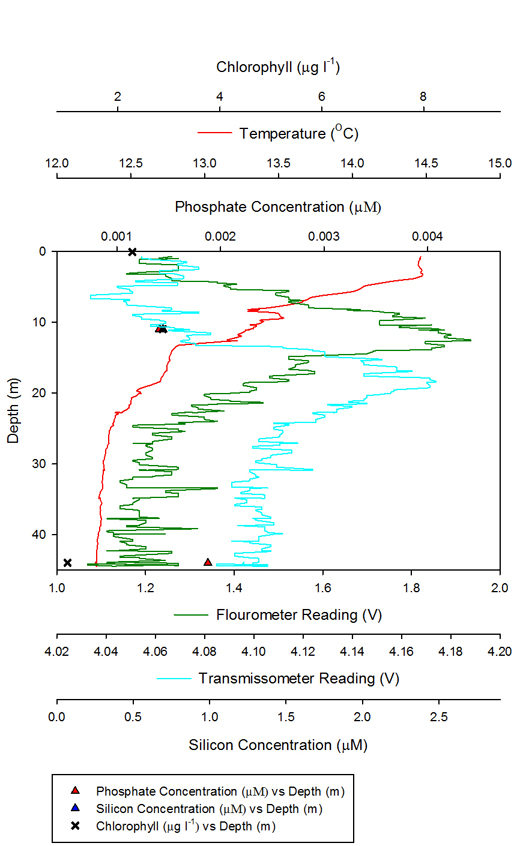
Station 7 Station 7 (lat: 50º 00.321, long: 5º 04.417) at 13.39GMT shows a variation in temperature of 2°C from depths of 5m to 15m. Below 20m, temperature variation is negligible. The peak fluorometer reading occurs well within the euphotic zone at a depth of 12m. A peak in the transmissometer reading occurs below this at a depth of 18m, possibly due to the elevated presence of zooplankton below the phytoplankton peak.
|
||||||||||
| |
|||||||||||
|
|
Station 8 Station 8, representing the same position as Station 1 at high tide (17.10GMT), shows a deepening in the thermocline, equal to that of the additional tide height of 3m. This thermocline is more defined at a depth of approximately 11m. The transmissometer readings show little variation over depth at both Stations. Chlorophyll values here do not show any correspondence to the fluorometer peak readings.
|
||||||||||
| ADCP | |||||||||||
|
|
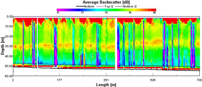
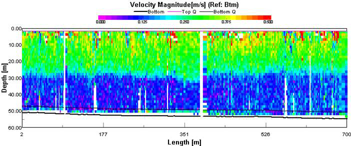
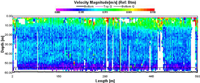
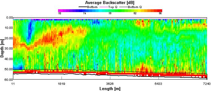
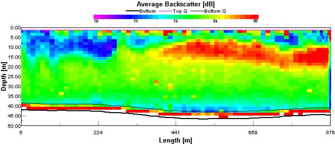
Station 2 (fig 4.6) shows high levels of shear stress at around 30m depth between the slower moving bottom layer and faster moving surface layer. The Richardson number (Ri) was 0.03 across this boundary layer. This is much lower than 0.25 and therefore indicates instability and mixing across the shear layer. This mixing between layers brings up nutrients into the surface layer allowing phytoplankton and zooplankton to bloom. Their presence causes a high level of backscatter at this depth. The layer of backscatter seems to take the form of an internal wave. These are normally caused by differences in density between two layers of water. They can be initiated by anything from tidal flow to the Ekman spiral both of which could be causing the one observed on our ADCP profile at Station 2. Station 3 shows a more gradual change in flow velocity between the surface layer and flow at depth. This may be due to weaker stratification as seen in fig 4.7. The largest change in temperature occurs in the top 15 metres, deeper readings show a more gradual change in temperature down to the sea bed. This change in temperature gradient coincides with the move into the well mixed layer, as shown in the ADCP (fig 4.7). This is expected as Station 3 is located closer to the mouth of the estuary, so mixing is expected to be greater, due to increased tidal flows. The ADCP profile from Station 3 to Station 4 shows increased backscatter at 10- 30m depth from 0- 2000m from the Station 3 end of the transect (See Fig. 4.8). When viewed against the CTD data, this is supported by an increase in both the fluorometer voltage and transmissometer reading (See Fig.??). This is due to higher particulate matter in the water column, which may be indicative, primarily, of the presence of zooplankton.
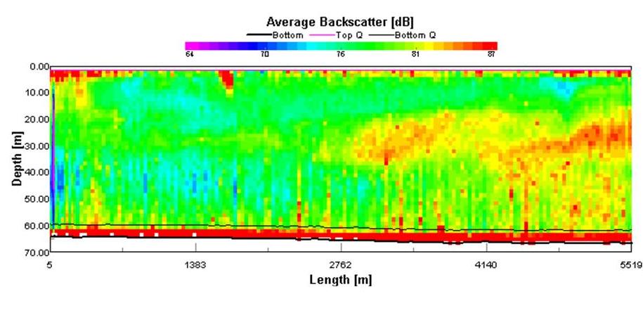
The ADCP profile from Station 4 to Station 5 shows an increase in backscatter at a depth of approximately 20-30m from 3000m towards the end of the transect. This is supported by the Station 5 CDT data as in Fig. 4.9 which shows increased flourometer voltage and transmissometer readings. From the increased transmissometer reading 10m below this backscatter peak it could be concluded that the increased backscatter was due to the increased presence of zooplankton.
The profile from Station 6 to Station 7 indicated a higher backscatter between depths of 5 and 15m from 450m to Station 7. This is supported by the CTD data as shown in Fig. 4.10 which, as in previous profiles, shows an increase in both the transmissometer readings and flourtmeter readings, peaks of which occur at 20m and 12m respectively.
In conclusion there is an evident relationship between the position of zooplankton and phytoplankton indicated by both backscatter from the ADCP and CTD data. |
||||||||||
| |
|||||||||||
|
|
Phytoplankton |
|
|||||||||
| Station 1 – Simply a practice Station and has thus not been analysed for this website due to time constraints.
|
|||||||||||
|
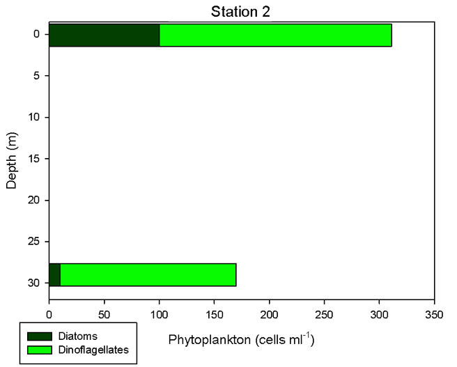
Fig
4.11 Phytoplankton group composition vs depth for Station 2
|
Station 2 – Dodman point (fig 4.11) Sampling from the surface waters gave a value of 311 cells/ml, with roughly two thirds of this being made up of dinoflagellates and the remaining third diatoms. The sample taken at 29m gave a much lower value of 170 cells/ml, with only 10 cells/ml being diatoms, and the remaining 160 cells/ml dinoflagellates.
|
|
|||||||||
| |
|||||||||||
|
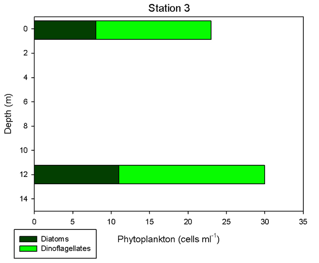
Fig
4.12 Phytoplankton group composition vs depth for Station 3
|
Station 3 (fig 4.12) Much lower surface and depth (12m) values were recorded at Station 3, with only 23 cells/ml and 30 cells/ml respectively. Both the surface and depth samples contained roughly half as many diatoms as dinoflagellates. The relatively low proportion of diatoms indicates that the main spring diatom bloom has already occurred, and that dinoflagellates are becoming dominant.
|
|
|||||||||
| |
|||||||||||
|
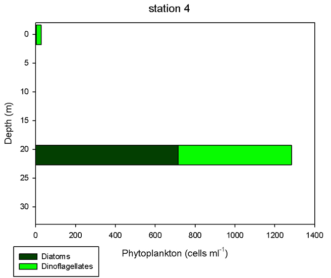
Fig
4.13 Phytoplankton group composition vs depth for Station 4
|
Station 4 (fig 4.13) A low surface value of 28 cells/ml was recorded, with only 3 cells/ml being diatoms. At 21m depth a deep chlorophyll maximum was observed this coincided with the thermocline. Very high values of phytoplankton were recorded here at 1284 cells/ml. Diatoms made up 56% of this sample, with the remaining 44% being dinoflagellates.
|
|
|||||||||
| |
|||||||||||
|
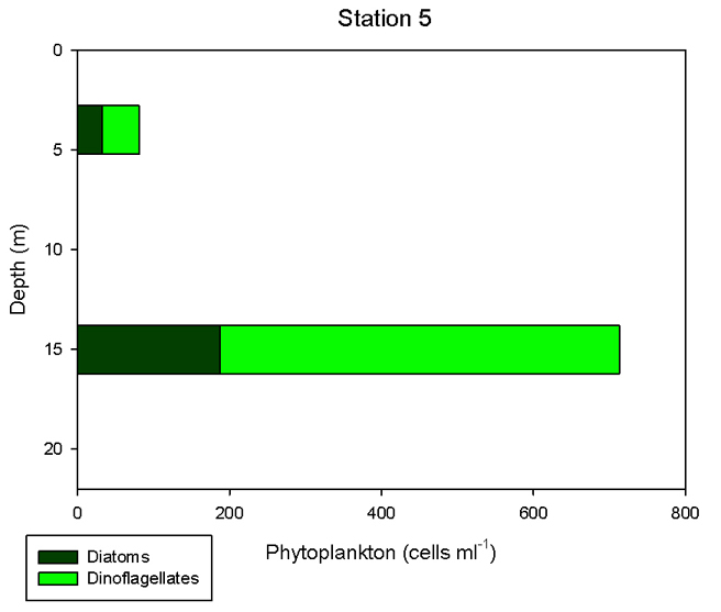
Fig 4.14 Phytoplankton group composition vs depth for Station 5
|
Station 5 (fig 4.14) The surface waters at Station 5 had relatively low numbers of phytoplankton at 81 cells/ml, 60 % dinoflagellates and 40 % diatoms. A deep chlorophyll maximum was also observed at Station 5, this gave very high values of 713 cells/ml in the sample taken from 15m. 74% of this value was dinoflagellates, with the remaining 26% diatoms. Deep chlorophyll maxima occur due to the stabilization of the water column as a result of thermal stratification. The development of phytoplankton blooms strip nutrients from the surface waters, causing phytoplankton to be most prevalent at the depth of the thermocline due to the cooler nutrient rich waters.
|
|
|||||||||
| Zooplankton (fig 4.15) |
|||||||||||
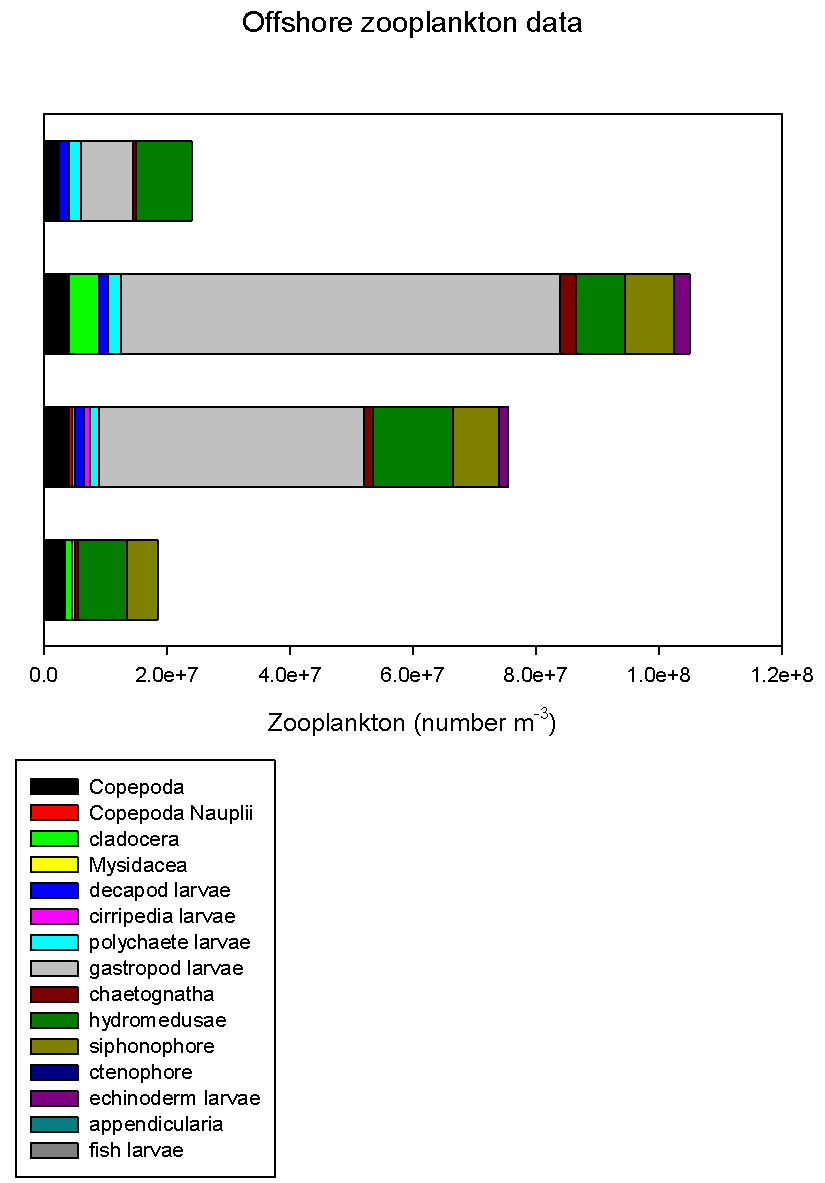 Fig 4.15 Zooplankton species composition for
Stations 2-5
Fig 4.15 Zooplankton species composition for
Stations 2-5 |
Station 2 – Dodman point This Station contained a relatively small amount of zooplankton, with a value of only 1.9x10⁷ zooplankton/m3. This was made up of copepods, cladocera, polychaete larvae, hydromedusae and siphonophores, with roughly 50% being hydromedusae.
|
||||||||||
| Station 3 7.6x10⁷ zooplankton/m3 were found at Station 3, a wider variety of species were recorded. Gastropod larvae made up roughly 60% of the sample, with copepods, copepod nauplii, cladocera, decapod larvae, cirripede larvae, polychaete larvae, chaetognaths, hydromedusae, siphonophores and echinoderm larvae making up the remaining 40%.
|
|||||||||||
| Station 4 The largest number of zooplankton was recorded at Station 4, with 1.1x10⁷ zooplankton/m3. 70% of the sample was made up of gastropod larvae, with the remaining 30% being made up of copepods, cladocera, decapod larvae, polychaete larvae, hydromedusae, siphonophores and echinoderm larvae. The large number of zooplankton observed here corresponds with the high concentration of phytoplankton also found at Station 4.
|
|||||||||||
| Station 5 A relatively low value of 2.4x10⁷ zooplankton/m3 was recorded at Station 5. Roughly 70 % of the sample was made up of equal numbers of hydromedusae and gastropod larvae. The remaining 30% was made up of copepods, decapod larvae, polychaete larvae and chaetognaths.
|
|||||||||||
| Conclusion |
|||||||||||
|
The aim of the offshore survey; to determine the degree of stratification within the water column following high wind conditions and in addition, attempt to locate a previously located front in the area, was completed. Although an attempt was made, a front was not located, possibly due to the preceding weather conditions having caused its position to move. Stations 1, 5 and 7 show a high degree of thermal stratification along with peaks in chlorophyll levels at the thermocline, or deep chlorophyll maxima. At Station 2 the ADCP showed high levels of shear stress at a depth of 30m, this marks the boundary between the slow moving deeper waters and faster moving surface waters. Instability and mixing between the two layers are suggested by a very low Richardson of 0.03. Zooplankton were successfully located by the presence of large areas of backscatter located below the chlorophyll maxima. Phytoplankton were most abundant at the thermocline, with relatively small numbers present in the surface waters. |
|||||||||||
|
|
|||||||||||
|
Chlorophyll,
dissolved Phosphate and Silicon were analysed manually in the lab using
the method according to Parsons et al (1984)Analysis
of dissolved oxygen was carried out following the method laid out in Grasshoff
et al (1999). Flow
injection analysis of nitrate was carried out according to Zooplankton samples were preserved using formalin, and concentrated down to 150ml. The samples were thoroughly mixed before 2ml was added to a Bogorov tray for analysis under a light microscope. Phytoplankton samples were preserved using Lugol’s solution. The phytoplankton settled out over night, and the 100ml samples concentrated to 10ml. 1ml of each sample was added to a Sedgwick-Rafter cell for light microscope analysis.
|
|||||||||||
|
|
|||||||||||
| Parsons T. R. Maita Y. and Lalli C. (1984) “ A manual of chemical and biological methods for seawater analysis” 173 p. Pergamon.
Grasshoff, K., K. Kremling, and M. Ehrhardt. (1999). Methods of seawater analysis. 3rd ed. Wiley-VCH
Johnson K. and Petty R.L.(1983) “Determination of nitrate and nitrite in seawater by flow injection analysis”. Limnology and Oceanography 28 1260-1266 Langston, W.J. et al 2003, Characterisation of European Marine Sites,
The Fal and Helford (Candidate) SAC, Marine Biology Association Occasional
Publication, No. 8
|
|||||||||||
| Roles | Disclaimer | |
|
Website Manager – Jenny Cook |
The opinions and views expressed on this website do not represent those of the National Oceanography Centre or the University of Southampton |


