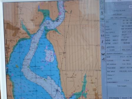
| Vessel |
Equipment |
Information |
Aims |
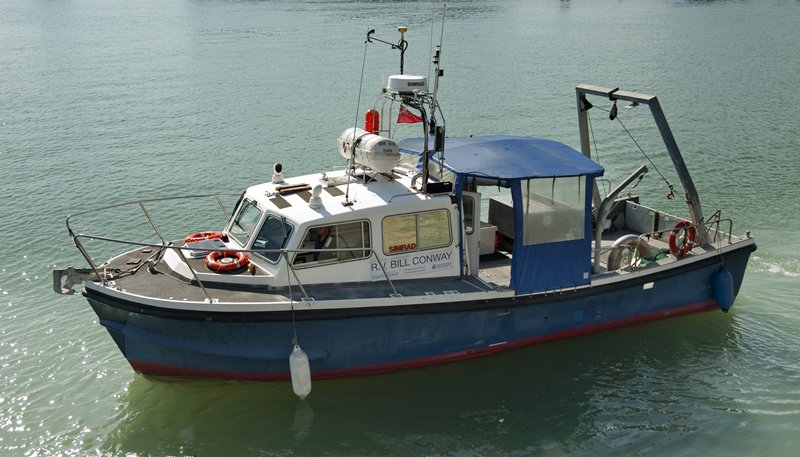
| RV Callista |
-
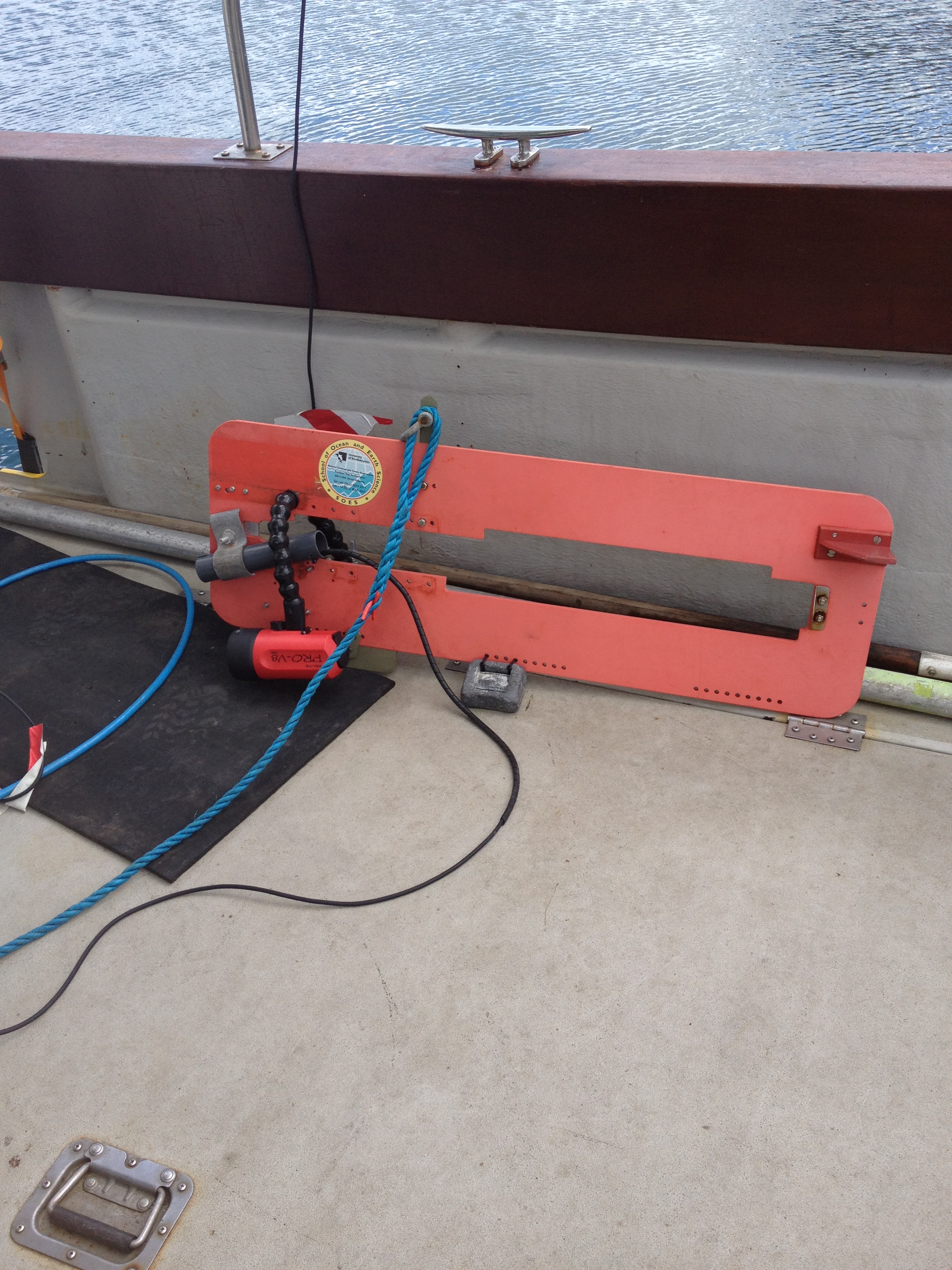
Vertical
plankton net
-
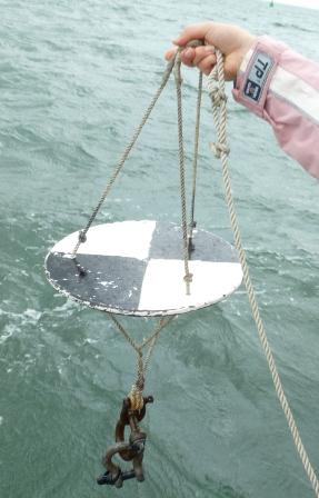
Secchi
disk
-
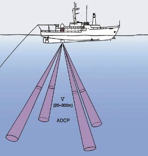
ADCP
-
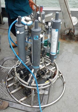
CTD
-
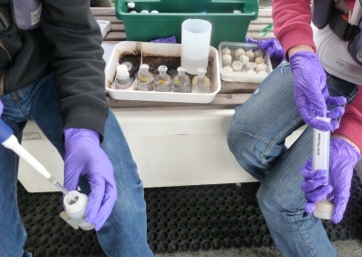
Chemical
analysis
|
-
Date:
3/7/2012
-
Weather:
Light continuous rain
-
Wave
height: 1m to 1.5m
-
Cloud
cover: 8/8
-
Air temperature: am-15.0
°C,
pm-14.6°C
-
Tides: Low
water 12.10 GMT
-
Wind speed: am- 19.5 knots
direction: 172°,
pm- 21.2 knots direction: 169.9°
-
Sea
surface: big swell
|
The aim of the offshore boat work was to carry out a time series
with
successive time intervals spaced half an hour apart. |
|
Methodology
In order to achieve our aim, it was decided
to choose a sheltered position and anchor there in order to
carry out measurements. Although an idea of the position was
discussed prior to the boat work, the final position was not
determined until just before departure after discussion with the
skipper. The objective was to take an ADCP transect on the way
towards our position and another one on the way back in order to
try and look at the flow before and after low water. Upon
reaching our station a CTD profile was to be taken every half an
hour in order to see
changes in
chlorophyll, turbidity, salinity and temperature and to take
water samples from the CTD every hour for chemical analysis of
silicon, nitrate, phosphate, chlorophyll and oxygen.
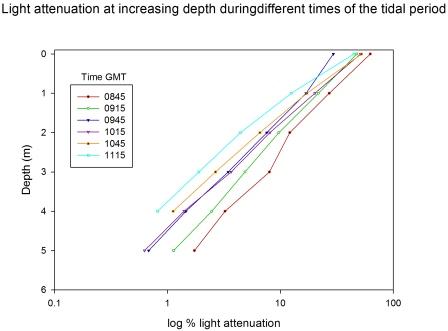
A secchi
disk reading was also to be taken every hour to give an idea of
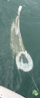
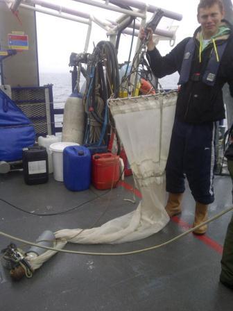
changing light attenuation and a vertical plankton net was also
to be taken hourly at different depths depending on the
backscatter.
The
R.V Callista departed at 07.45 GMT, and headed towards Black
Rock to perform a CTD at the location 50
°10.111
N, 005° 02.488 W where 5 bottles were taken at depths 20m, 14m, 8m,
4m and 1m. This was in order for cross calibration with the
group on the R.V Conway. A secchi disk and plankton net between
20m depth and the surface were also taken at this station. We
then moved on to the predetermined position chosen for our time
series station, located about 1 mile of Porthouse stock at 50° 03.845 N, 005°
02.782 W. On the way to the station an ADCP transect
was performed
in order
to look at changes in flow and the backscatter. The transect
began at 08.51 GMT at 50° 09.313 N, 005°
01.919 W and ended at 09.29 GMT at position 50° 08.629 N, 005°
01.403 W.
Upon reaching our chosen location, the Callista dropped anchor
to secure itself in position. The first CTD was taken at 11.17
GMT and 5 sample bottles were taken. Chemical analysis was then
carried out on each bottle and a sample for nitrate, silicon,
dissolved oxygen, lupus iodine and two chlorophyll were taken.
The CTD was then lowered and data recorded every half an hour at
11.17 GMT, 11.55 GMT, 12.20 GMT, 12.38 GMT, 13.19 GMT and 13.43 GMT with
water bottle samples being taken hourly at 11.17 GMT where 3
bottles were taken, 12.20 GMT where 3 bottle samples were
collected and at 13.19 GMT where 4 bottles were taken and chemical analysis was carried out for each.
A secchi disk
reading was also taken every hour at 11.17 GMT, 12.20 GMT, 13.19
GMT and the distance from the disk to surface of the water
measured using markings on the rope. A further two repeats were
then taken to ensure accuracy. A vertical plankton net was also
taken hourly. The first net was taken at 11.35 GMT where two
samples were taken between depths 25m and 15m and 15m and the
surface, the next at 12.34 GMT where again two samples were
taken between depths 30m and 20m and 20m and the surface and
finally at 13.28 where one samples was taken between 20m and the
surface. The plankton net had a diameter of 60.3µm and a mesh size of 200µm.
The final CTD reading was recorded at 13.55 GMT and the anchor
brought up. We began to return back to the harbour on the way
taking the second ADCP transect which began at 14.18 at 50°
03.806 N and 005° 02.675 W and ended at 15.01 GMT at 50°03.806 N
and 005°01.588 W.
|
|
Results |
|
Physical |
ADCP |
 |
 |
 |
 |
|
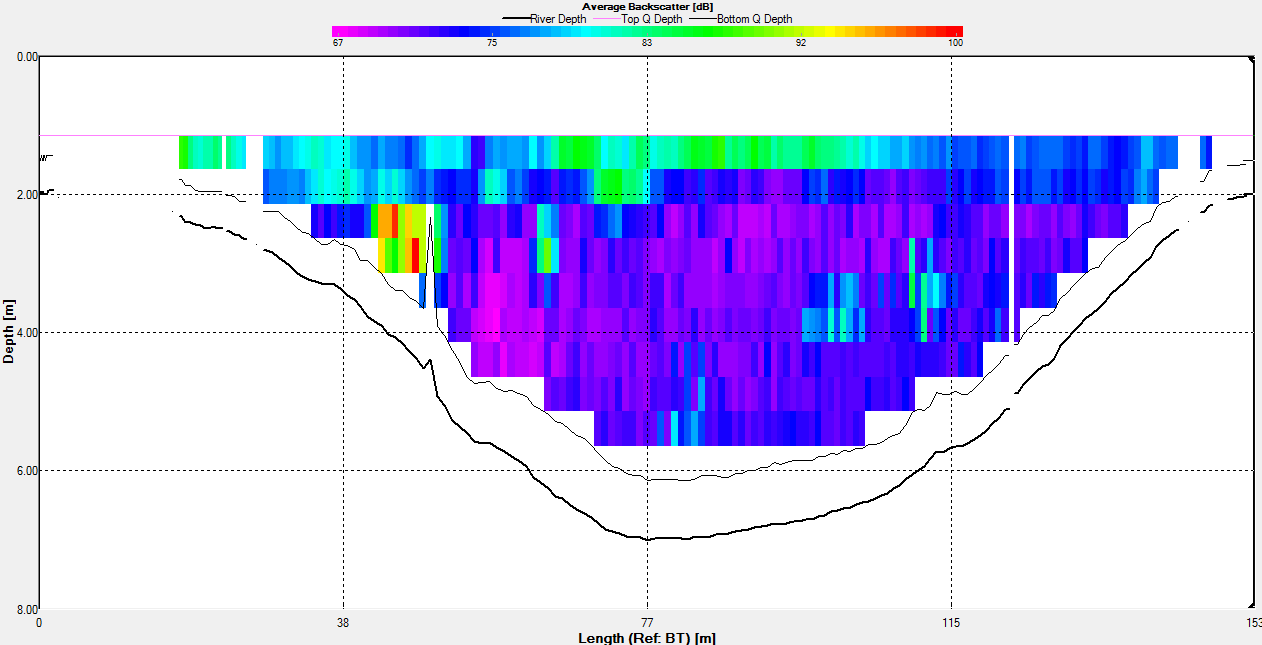
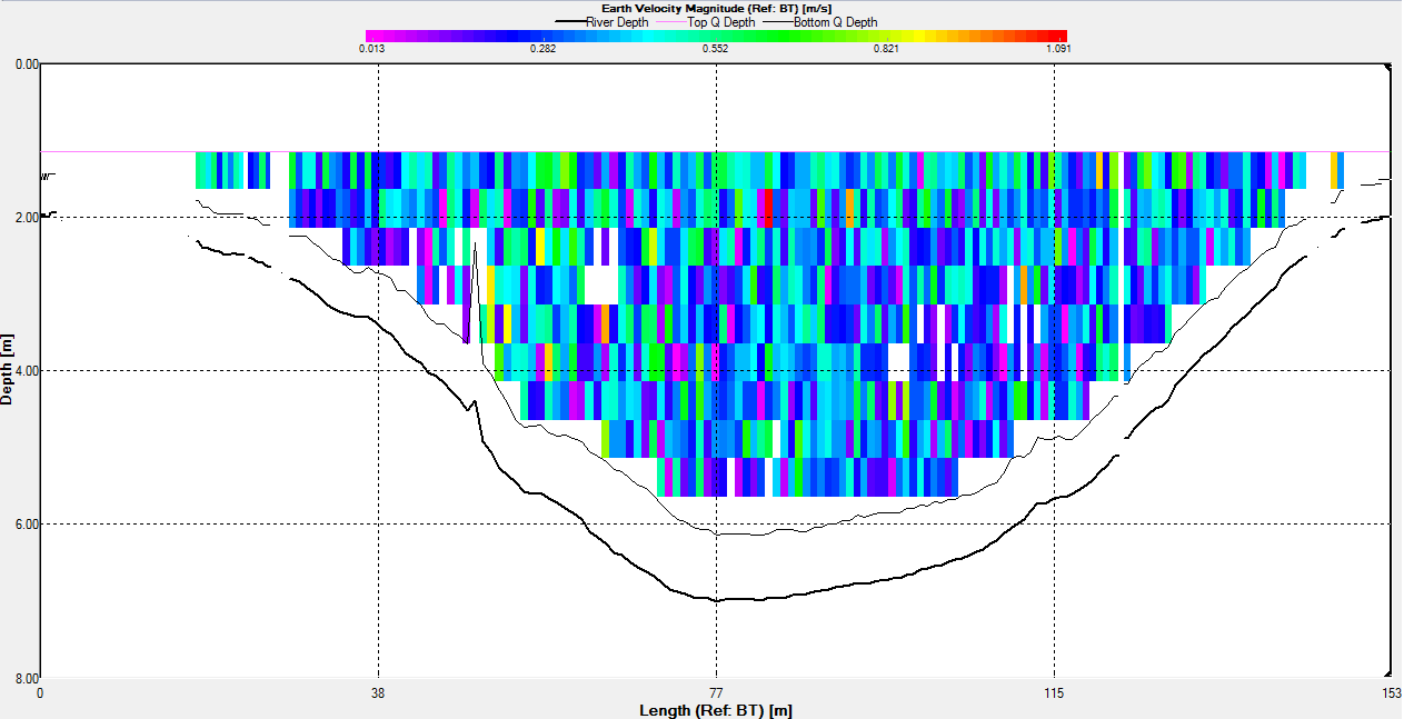
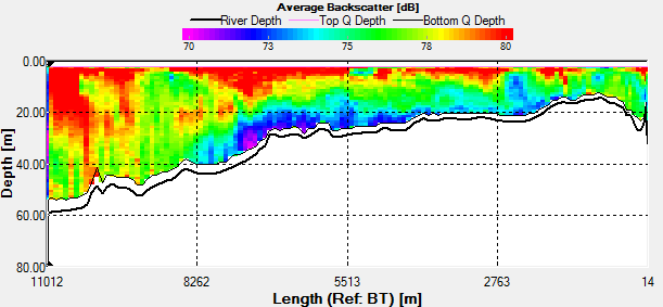
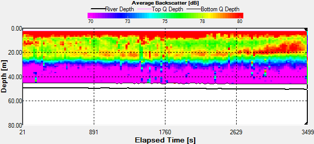
Fig. 44 - Station 3a
Backscatter |
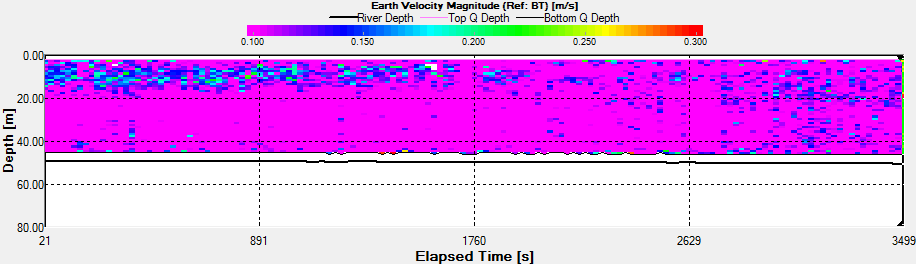
Fig. 45 - Station 3a
Velocity |
 |
 |
 |
 |
|
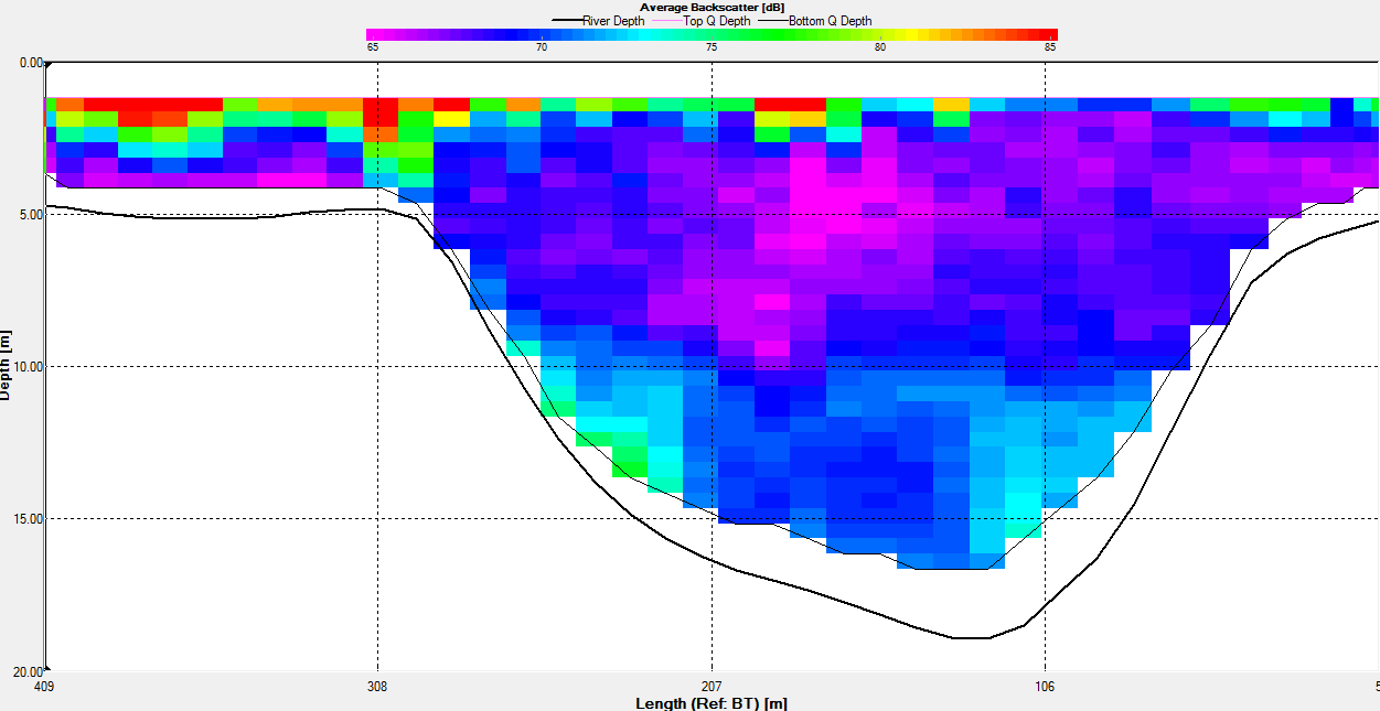
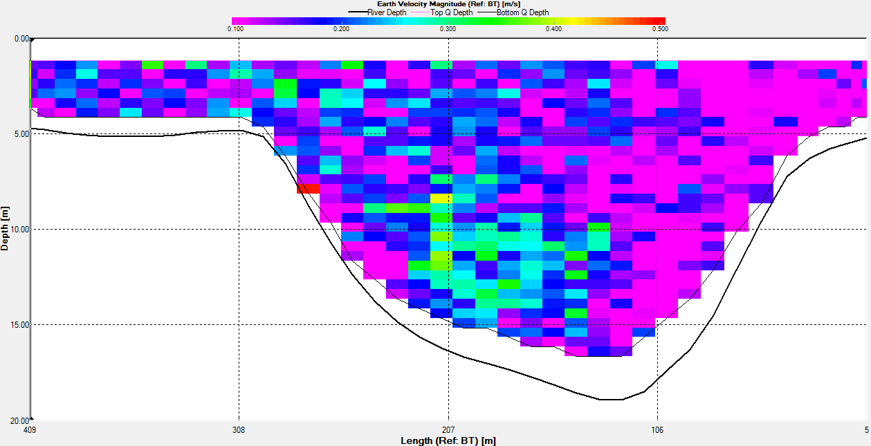
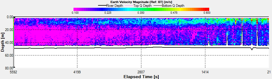
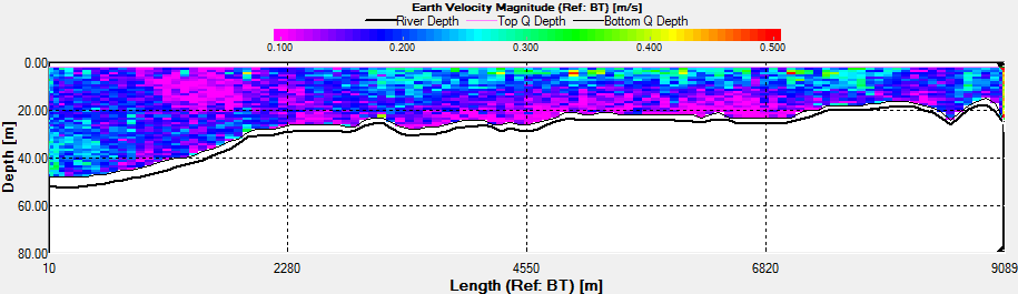
Fig. 46 - Station 3c
Backscatter |
Fig. 47 - Station 3c
Velocity |
 |
 |
 |
 |
|
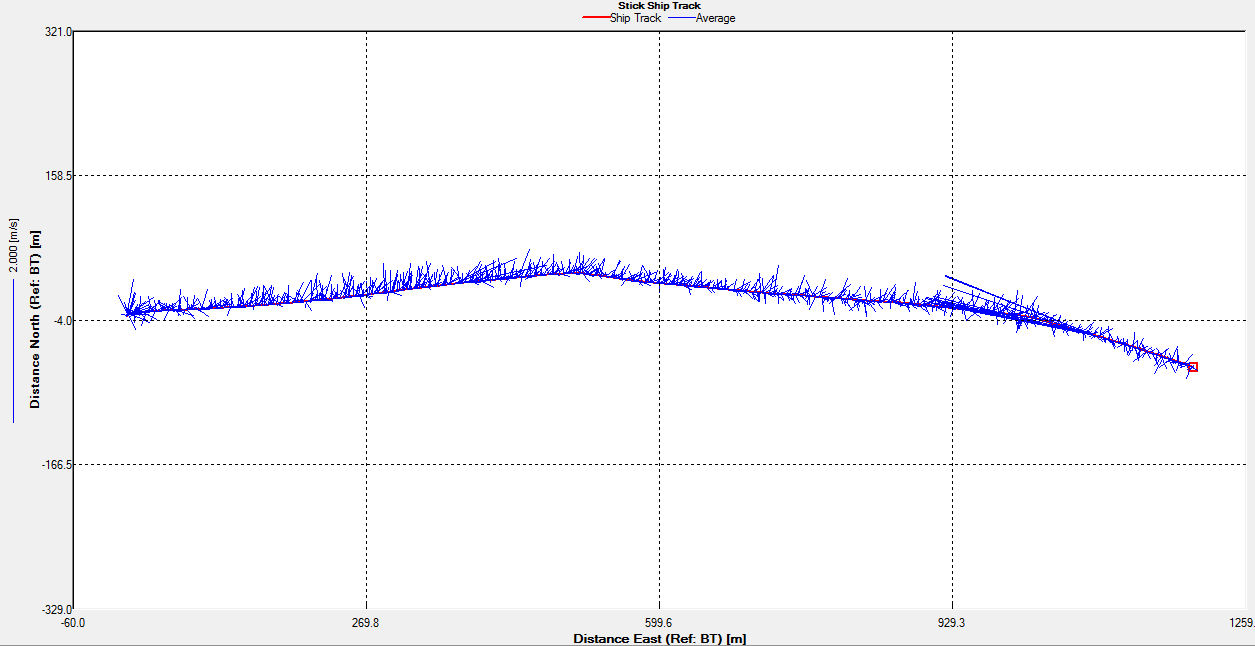
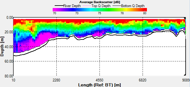
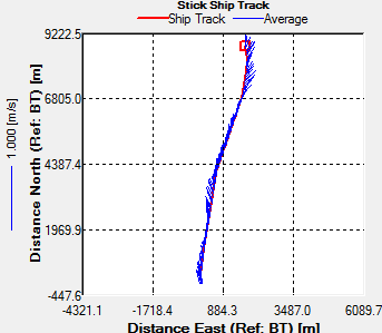
Fig. 42 - Transect 1
Backscatter, Shiptrack and Velocity |
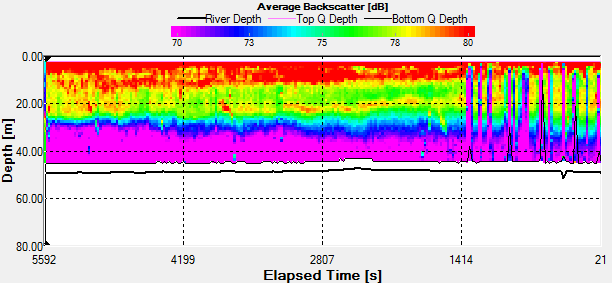
Fig. 43 - Transect 2
Backscatter, Shiptrack and Velocity |
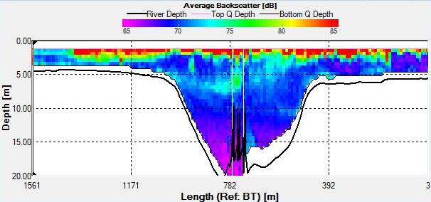
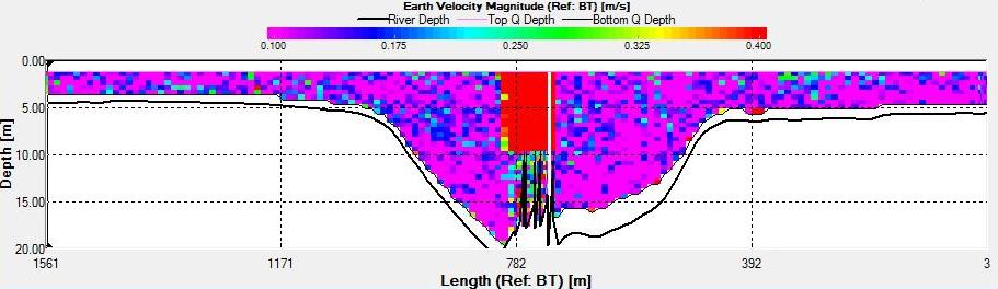
Fig. 48 - Station 3e
Backscatter |
Fig. 49 - Station 3e
Velocity |
|
|
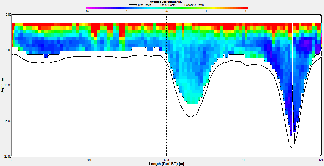
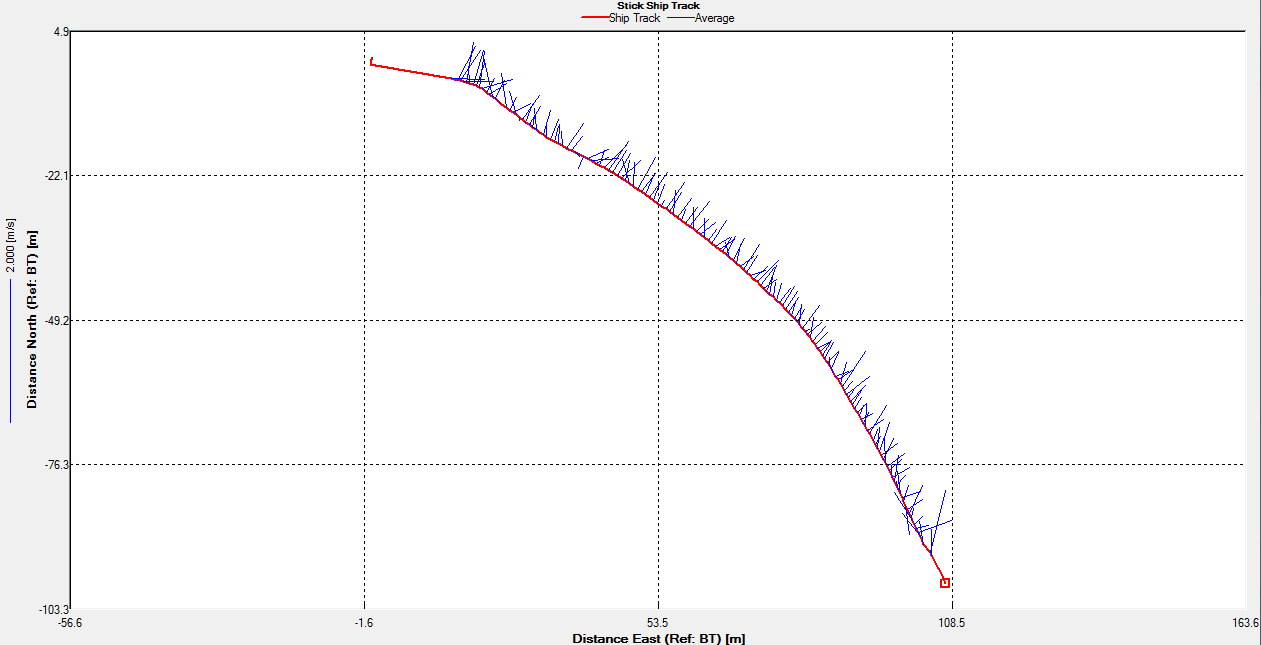
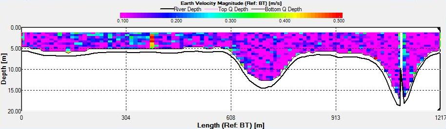
Transect 1 was taken from Black Rock to
Station 3 (the location of the time series) before low water.
The direction of flow of the tide going out can be seen on the
ship track flowing in a southward direction (Fig.42). There is a
change in velocity magnitude over the transect, we can see a
general increase from 0.1m/s to 0.5m/s as the water gets deeper.
The increase is caused due to acceleration around the headland,
and is not due to any shear after looking at the direction of
flow. |
|
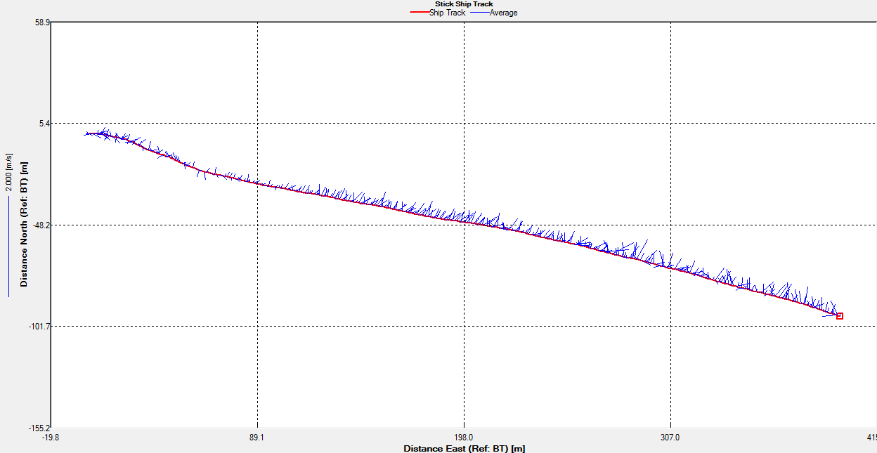
Transect 2 was taken along a similar track
going from Station 3 to Black Rock. This transect was taken
after low water, as shown from the direction of flow northward
on the ship track (Fig.43). The velocity magnitude doesn’t vary
much between 0.1m/s and 0.3m/s. Again there is a higher velocity
where the water is accelerated around the headland. Also the
velocity is greater at the surface which may be due to wind
forcing and the swell which was coming in from the south west.
|
|
Transect 1
– before low water |
Transect 2
– before high water |
|
Time (start, end) |
0933GMT,
1025GMT |
Time (start, end) |
1418GMT, 1501GMT |
|
Start location (Lat,
Long) |
50°09.313N,
005°01.919W |
Start location (Lat,
Long) |
50°03.860N, 005°02.75W |
|
End location (Lat, Long) |
50°02.700N,
005°01.970W |
End location (Lat, Long) |
50°08.785N, 005°01.588 |
|
Length of transect |
11011.72m |
Length of transect |
9089.46m |
|
|
There is high amount of backscatter from
Transect 1 (Fig.42). The values close to the surface are likely
to be due to zooplankton as there is a chlorophyll maximum
around 10m depth. There are high amounts of backscatter
corresponding to the high velocities. The backscatter therefore
is most likely due to bubbles in the water column and not
biological activity. Transect 2 shows a more constant high
backscatter at the surface, which clearly corresponds to the
chlorophyll maximum, so is most likely to be caused from the
zooplankton (Fig.43). As this transect was taken at towards high
water, where phytoplankton flood into the estuary, zooplankton
are likely to follow. |
|
Station 3a |
|
Time (start, end) |
1040GMT, 1214GMT |
|
Start location (Lat,
Long) |
50°03.834N,
005°02.697W |
|
End location (Lat,
Long) |
50°03.847N,
005°02.789W |
|
Station 3c |
|
Time (start, end) |
1214GMT, 1313GMT |
|
Start location (Lat,
Long) |
50°03.847N,
005°02.789W |
|
End location (Lat,
Long) |
50°03.849N,
005°02.772W |
|
Station 3e |
|
Time (start, end) |
1313GMT, 1358GMT |
|
Start location (Lat,
Long) |
50°03.849N,
005°02.772W |
|
End location (Lat,
Long) |
50°03.843N,
005°02.748W |
|
|
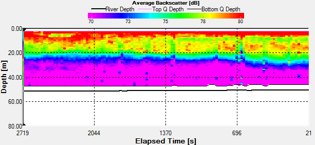
The Station
3a time series was taken the period before during and the hour
after low water low water. In the backscatter contour there is
an area of error from the ADCP where there were bad
values(Fig.44.). But the values stay fairly constant showing
zooplankton sat in the top 10m. There is an increase with depth
also through time, suggesting that the zooplankton are
migrating. There are a few anomalies in the backscatter, for
example 3700s into the series there is a high amount of
backscatter at 20m depth. This may be due to bubbles in the
water, but as nothing suggests this from the velocity magnitude
contour, it could also be down to a collection of zooplankton or
a shoal of fish. There is a slight decrease in velocity with
time over the entire water column, but is most apparent in the
top 10m of the water column from 0.350m/s to 0.120m/s.
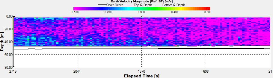
The Station
3c time series was taken 2hours after low water. The backscatter
contour indicates again that zooplankton is sat in the top 10m
of the water column(Fig.46). After 2800s into the series there
is an increase in backscatter between 12m and 20m. Again this
may be due to migration of zooplankton. There is little change
in velocity over the time period, with it mainly being 0.1m/s.
The Station 3e series shows the further change towards high
water after the last station. There is a high backscatter in the
top 10m still, with additional around 15m (Fig.48). The velocity
increases with time through the water column as the tide
continues to come in. |
|
CTD |
|
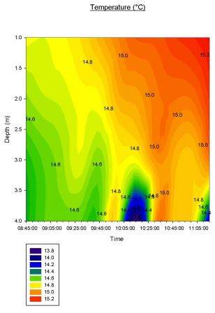
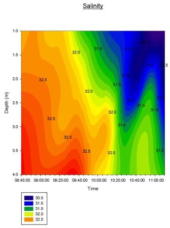
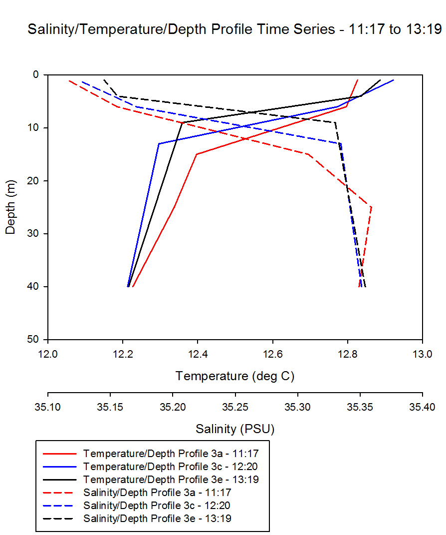
Figure 50
shows the temperature and salinity depth profiles we obtained
using the CTD during the time series.
The first
profile was done at 11:17, followed by 12:20 and then 13:19.
Knowing that low tide was 12:10, we decided that a time series
over the low tide time would provide an interesting profile.
Looking at the
graph, we can see that as time advances, the depths of both the
thermocline and the halocline becomes shallower, rising from
approximately 15m to 10m. The thermocline becomes shallower due
to solar radiation, with a difference of about 0.6oC.
This increases stratification, thus reducing the depth of the
thermocline.
The graph also
shows a distinct halocline with a difference of about 0.2 PSU.
This is a result of both fresh water input from the rivers Fal
and Helford, and from the large amount of rainfall that fell
around the time of our data collection. Less dense relatively
fresh water is trapped between the surface and the thermocline.
|
 |
|
Fig. 50 - CTD Depth Profile
Time Series |
|
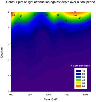
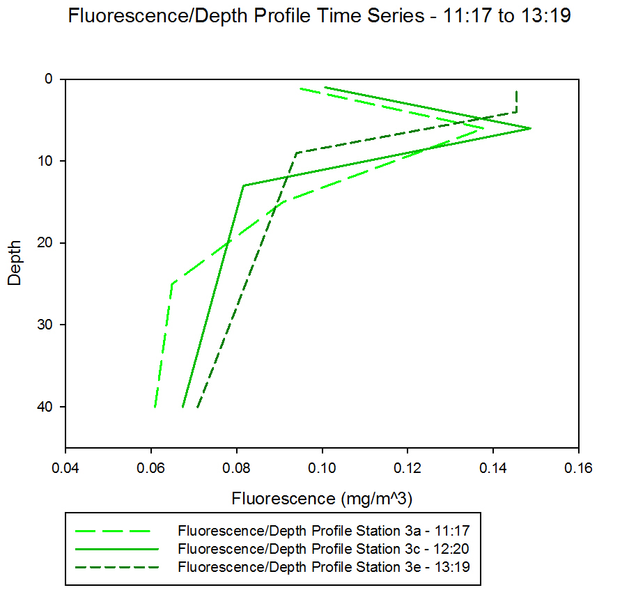
Figure 51 shows the
fluorescence profiles through a time series at Station 3.
Fluorescence is a
function of chlorophyll, and it is possible to determine the
location of the chlorophyll maxima by using the fluorescence
data. There is a very sharp gradient that rises from 26m to 10m
over the course of the time series. This is a result of the
movement of the thermocline, as discussed above.
The chlorophyll
maxima will follow the thermocline as the phytoplankton
containing chlorophyll cannot mix below the thermocline.
Interestingly, we also see an increase in fluorescence over the
time period also. This is a result of the concentration of
chlorophyll increasing.
As the thermocline
becomes shallower, the phytoplankton are trapped in a smaller
and smaller volume, and so the concentration of chlorophyll
increases, thus increasing fluorescence.
|
 |
|
Fig 51 - Chlorophyll Depth Profile
Time Series |
|
Richardson Number |
|
|
 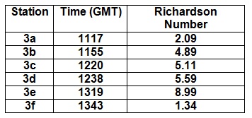 |
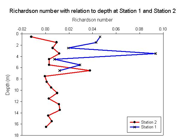
The table in figure
52 shows the Richardson Numbers for each station, where the
whole water column has been treated as a single layer. These
values show an increasing stability from 1117GMT to 1319GMT and
then a drop in stability at 1343GMT. Low water was at 1110GMT.
This meant that the tide was in flood at all the stations, which
caused a layer of lower salinity water at the top of the water
column, as seen in the salinity profile graph. This lower
salinity layer causes salinity and therefore density
stratification in the water column with increasing stabilisation
through time as the flooding layer increases.
Station 3a has a lot
of negative values due to the densities of the top layers being
slightly larger than the bottom layers. Station 3a was taken
about 10 minutes after low water, therefore the water column
density appears homogeneous with depth due to the change in tide
direction during low water. This is the reason for the potential
mixing due to the denser water being above the less dense water.
This homogenous water column causes very similar densities in
the layers within the water column. This causes some of the
Richardson Numbers to be negative as they have slightly larger
densities in the top of the layer, these differences in density
are insignificant as they are ±0.001kgm-3. Station 3a
has a vorticity of 3.72x10⁻³s-1
and a period of 268.74s.
Station 3c shows more
stability than Station 3a. This increase in stability is due to
the continuous flooding of the tides and increasing stability.
This station has a vorticity of 4.50x10⁻³ and a
period of 221.91s.
Station 3e was taken
two hours after low tide. It has the highest Richardson Number
of all the stations - 8.99. This suggests the water column was
very stable compared to the other stations, which is again due
to the flooding tide increasing the density stratification.
There is a stability peak within the layer at 27m, this is most
probably due to a reduction in velocity values recorded by the
ADCP. Station 3e has a vorticity of 6.38x10⁻³ and a
period of 156.65s. |
|
Biological |
Chlorophyll |
 |
 |
|
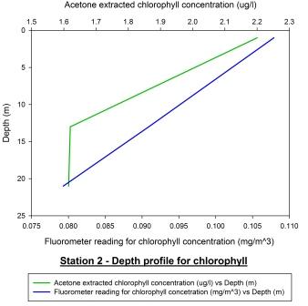
Fig 53 - Station 2
Depth Profile |
Fig 54 - Station 2
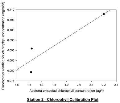
Calibration Plot |
 |
 |
|
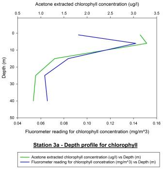
Fig 55 - Station 3a
Depth Profile |
Fig 56 - Station 3a
Calibration Plot |
 |
 |
|
Fig 57 - Station 3c
Depth Profile |
Fig 58 - Station 3c
Calibration Plot |
 |
 |
|
Fig 59 - Station 3e
Depth profile |
Fig 60 - Station 3e
Calibration Plot |
|
Our offshore
study took place over a period of 3 hours covering the low water
period. This gave us a detailed data set on how the water
column changed with time over a period of low water.
Figure 52 displays
the depth profile for chlorophyll at Black Rock. It shows both
profiles for acetone extracted chlorophyll samples and
fluorometer calculated concentrations. Both profiles appear to
correlate well and follow a similar pattern of decreasing
chlorophyll concentration with depth. The data shows a
chlorophyll maximum at the surface of the water column at 1m
suggesting a large population of phytoplankton occupy this
particular depth. As phytoplankton are photosynthetic organisms,
it would be expected that they reside in the upper most layers
of the water column where light penetration is at its maximum.
As the depth of the water increases, the light level decreases;
therefore lowering the potential for photosynthetic output and
so the concentration of chlorophyll is lower due to a lack of
phytoplankton. Figure 53 shows the calibration plot for station
2. Although the two profiles seem to follow a similar pattern
and the calibration plot appears to have some correlation, a
Pearson Product Moment Correlation test revealed the P value to
be >0.050 and so there is no significant relationship between
the two profiles. Acetone extracted chlorophyll samples are
considered more accurate as there can often be calibration
problems with fluorometers.
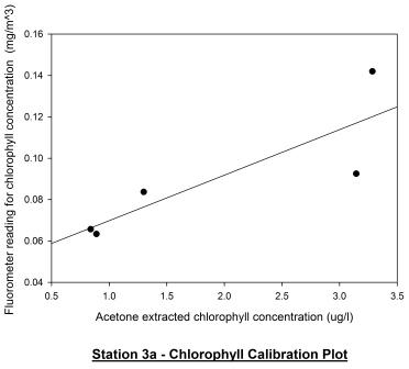
Station 3a
(1117GMT) shown in figure 54 represents the chlorophyll depth
profile for our station approaching low water. Acetone extracted
chlorophyll sampling is considered a more accurate method of
sampling chlorophyll concentration and so these are the
measurements used in this analysis. There appears to be a
chlorophyll maximum at 6 metres of around 3.3ug/l. This would
suggest the presence of a large bloom of phytoplankton.
Phytoplankton occupy shallower depths in the water column due to
their photosynthetic nature. Populations of phytoplankton are
rarely found in deeper waters as there is not sufficient light
for photosynthesis to occur. This then explains why chlorophyll
concentration then decreases as depth increases; reaching a
minimum of around 0.8 ug/l at 40m. This profile is also
reflected in the fluorometer profile however when looking at the
calibration plot shown in figure 55, there appears to be a
considerable amount of variation within the two profiles and
further analysis by the use of a Pearson Product Moment
Correlation test. This revealed that there was no correlation
between the two profiles as P > 0.050. This may be due to poor
calibration of the fluorometer which is a common problem; this
is why acetone extraction is considered a more reliable and
accurate method.
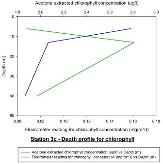
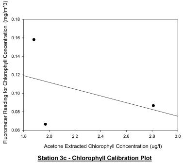
Station 3c
(1220GMT) shown in figure 56 displays the chlorophyll depth
profile just 10 minutes after low water (1210GMT). Looking at
the acetone extracted chlorophyll profile, it appears that the
chlorophyll maximum has increased in depth from 6m to 13m. The
chlorophyll maximum concentration decreased from 3.3 ug/l to
around 2.8 ug/l. This evidence suggests that the phytoplankton
may be migrating within the water column with the tidal cycle as
a stimulus and are possibly epipelic algae; phytoplankton that
are free living within the water column and migrate with tidal
cycles. The fluorometer profile appears to contradict the
acetone extracted profile. The calibration plot for station 3c
shown in figure 57 displays no correlation between the two
profiles which is further supported by a Pearson Product Moment
Correlation test. This test revealed there was no correlation
between the two profiles as P > 0.050.
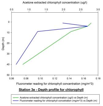
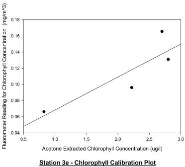
Station 3e
(1319GMT) shown in figure 58 represents the chlorophyll depth
profile approximately 1 hour and 9 minutes after low water
(1210GMT). It appears that the chlorophyll maximum has
decreased in depth from 13m to 1m, remaining at a value of
2.8ug/l. This may be due to phytoplankton migration towards the
surface as the tidal cycle moves from low water to high water.
The fluorometer profile shows a chlorophyll maximum of similar
magnitude at the same depth and appears to follow the same
pattern as the acetone extracted profile just slightly more
exaggerated; chlorophyll concentration decreases as depth
increases after the chlorophyll maximum. Figure 59 shows the
calibration plot for this station and although the plots seem to
have an obvious positive correlation, a Pearson Product Moment
Correlation test reveals that P > 0.050 and so there is no
significant relationship between the two profiles.
In conclusion
it appears that the chlorophyll maximum seems to increase in
depth whilst approaching high water and then appears to move
closer to the surface after low water and towards high water.
The chlorophyll concentration appears to decrease towards low
water. Based on these profiles I would predict that chlorophyll
concentration may begin to increase closer to high water
although a full tidal cycle study would be needed to confirm
this.
|
|
Phytoplankton and Zooplankton Numbers |
 |
|
Fig 61 - Station 3a
Phytoplankton |
 |
|
Fig 62 - Station 3c
Phytoplankton |
 |
|
Fig 63 - Station 3e
Phytoplankton |
|
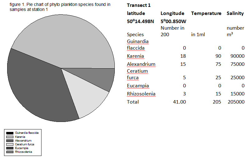
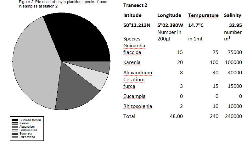
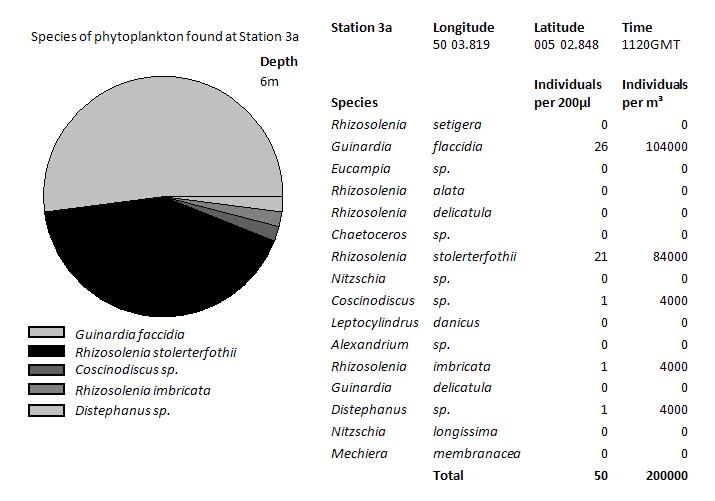
At depth 6m at
station 3a the highest phytoplankton numbers were found, with
200,000 per M3. The majority of the phytoplankton
species were domintated by the phytoplankton Guinardia flaccidia.
There was also large numbers of Rhizosolenia stolerterfothii
found.
In contrast, 15m depth there was little numbers of phytoplankton
found, just 10% of the numbers found 11m closer to the surface.
At this depth, different phytoplankton such as Rhizosolenia
imbricate are more dominant. However, Guinardia flaccidia, the
more dominant species from surface waters is still present. The
fact that Rhizosolenia imbricate dominate, indicates that they
are more adapted to lower light levels.
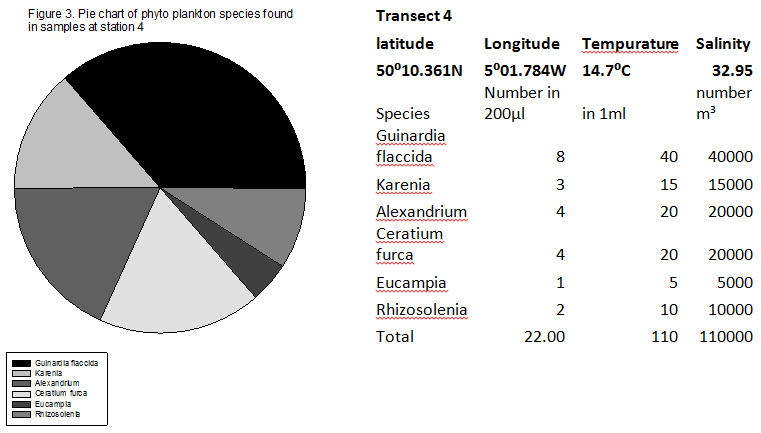
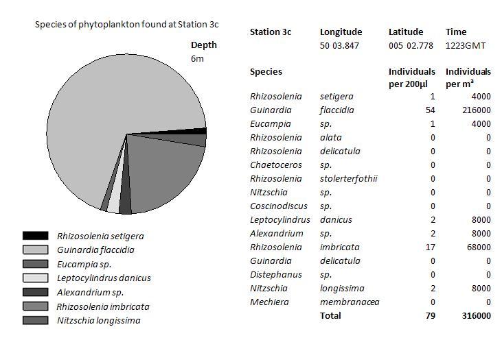
At 6m during station
3c, a large amount of phytoplankton were present with 316,000
present per m3. Once again, the dominant species at
this depth is Guinardia flaccida with around 2/3 of the species
found being this.
Station 3c at a depth
of 13m has a relatively low amount of phytoplankton present
compared to the waters above. The main species that do dominate
at these depths, as seen in 3a, is Rhizosolenia imbricata.
Guinardia flaccidia, Rhizosolenia alata and Rhizosolenia
stolerterfothii were all found in the same concentrations, half
of imbricate.
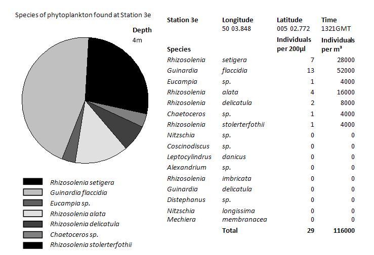
Although 3e, 4m,
showed the highest abundance of species per m3, it
still showed a lower total population than other stations (such
as 3a at 6m and 3c at 6m). The dominant species once again is
Guinardia flaccidia, with most Rhizosolenia species present,
apart from Rhizosolenia imbricate.
The dominant species
at this depth is Guinardia flaccidia which is surprising as the
dominant species found below the main phytoplankton band is
Rhizosolenia in all of our other stations. Rhizosolenia alata is
also present in large numbers, around 12000 per m3.
|
|
Chemical |
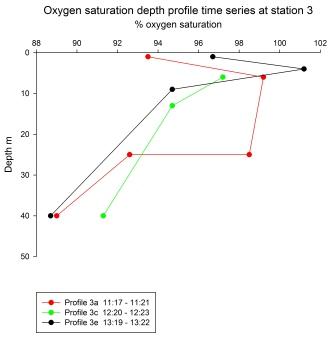 |
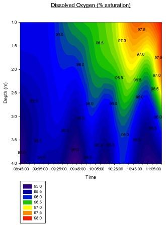
All three
depth profiles were taken at the same location using a
Niskin bottle rosette on a CTD. The profiles were each
done one hour apart.
Profile 3a
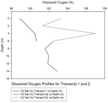
was the first to be taken. Oxygen is undersaturated
throughout the profile, with a maximum at 6 m (99.2%)
and a minimum of 89% at 40 m. Two samples were taken at
25 m, one was 92.6% saturated with oxygen and the other
98.5%. Only three samples were taken on profile 3c, the
surface sampled failed due to the misfiring of a Niskin
bottle. The profile shows a gradual decrease in % oxygen
saturation with depth, from 97.2 at 6 m to 91.3 at 40 m.
Profile 3e, like 3a, shows an oxygen saturation maximum
just below the surface at 4m, this is the only time and
place at which the water is supersaturated with oxygen
at 101.2%. Below this there is a gradual decrease in
oxygen saturation to 9 m, followed by a sharp reduction
in saturation to a minimum at 40 m.
All three
profiles show a general decrease in % oxygen saturation
with depth, with the exception of the maxima in profiles
3a and 3e at 6 and 4 m respectively. These depths
correspond with local chlorophyll maxima, so the high
oxygen saturation here is due to oxygen release caused
by phytoplanktonic photosynthesis. The decrease in
oxygen saturation beyond this depth is caused by the
respiration of zooplankton and other organisms, and the
lack of light minimising or eliminating the
photosynthesis which would reoxygenate these waters. The
difference in the two oxygen saturation levels at 25 m
on profile 3a is likely to be due to some form of error,
as it is very unlikely that water with such different
oxygen saturation should be so close as to be sampled
simultaneously by two Niskin bottles. |
|
Fig 64 - Oxygen
saturation at Station 3 |
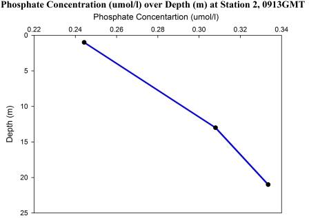 |
During the offshore investigation (03.07.12) water
samples were collected at intervals of 1hour. The aim
was to have a complete as possible illustration of the
water column in terms of chlorophyll, nitrate,
phosphate, dissolved oxygen and silicon in order to
build depth profiles of each parameter.
Phosphate analysis was carried out using the nitrate
water samples collected.
At station 2 (0913-0915 GMT), 3 water samples were
collected at 1m, 13m and 21m.
At station 3a (1117-1121 GMT), 4 water samples were
collected at 1m,6m,15m,25m and 40m.
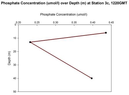
At station 3c (1220-1223 GMT), 3 water samples were
collected at 6m, 13m and 40m.
Finally, at station 3e (1319-1322 GMT), 4 water samples
were collected at 1m,4m,9m, and 40m.
The deepest collection points were restricted by the
respective topography of the station and the danger of a
potential crash of the CTD in the seabed. All phosphate
concentrations in figures are in µmol/l.
At station 2, the phosphate concentration increases
steadily with depth from 0.24µmol/l at 1m to 0.33µmol/l
at 21m of depth (figure 65). However, lack of water
samples between 1m and 13m renders it impossible to
support any claims of increase or decrease of the
phosphate concentration between these two depths similar
with the decrease found in station 3a at 6m (from 0.23
at 1m to 0.15 at 6m).
By comparing station 2 with station 3a (figure 66), a
phosphate enrichment is observed in the lower part of
the water column at 20-25m with values between 0.33-0.35
µmol/l. The upper water column (0-10m) is slightly
depleted with values ranging from 0.15-0.23µmol/l. A
possible explanation for this trend is that surface
phosphate enrichment from industrial plants and
agricultural wastes decreases with distant from the
estuary and higher concentrations are observed in the
lower part of the column as tidal currents remove
estuarine waters offshore.
At station 3c (figure 67), a phosphate maximum is
observed this time in the surface waters (0-10m,
0.43µmol/l) and a minimum at 13m (0.22µmol/l). The 40m
water sample has a value of 0.40µmol/l following the
trend of station 2 (figure 65) and station 3a (figure 66).
In conclusion, it is observed that the phosphate
concentration increases with depth in all stations and
the maximum phosphate concentration found is 0.45µmol/l
(figure 68) while the minimum is 0.15µmol/l (figure 66).
|
|
Fig 65 - Phosphate
concentration at Station 2 |
.JPG) |
|
Fig 66 - Phosphate
concentration at Station 3a |
 |
|
Fig 67 - Phosphate
concentration at Station 3c |
.JPG) |
|
Fig 68 - Phosphate
concentration at Station 3e |
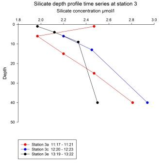 |
All three
depth profiles were taken at the same location, with one
hour between each.
Profile 3a
was the earliest taken. It shows the highest surface
silicate concentration of the three profiles, then drops
sharply to the lowest value for 5-6 m. After this
minimum at 6 m the silicate concentration steadily
increases with depth, reaching a maximum at 40 m at 2.81
µmol/l. Profile 3c has the lowest surface concentration
of silicate. The concentration gradually increases with
depth to 9 m, then rises more sharply to reach a maximum
at 40 m. No surface sample was taken for profile 3e,
this was due to a misfiring Niskin bottle. The profile
shows a gradual decrease in silicate concentration until
it too reaches a maximum at 40 m.
All three
profiles show a general increase in silicate
concentration with depth. This is because diatoms in the
sunlit surface waters remove silicate from the water in
order to build frustules – a “shell” which is rich in
silicon. As these diatoms die their heavy frustules sink
quickly and begin to be dissolved, increasing the
silicate concentration in the deeper waters. Here there
are no photosynthesising diatoms to take up the
dissolved silicate and so its concentration in deep
water remains high. The exception is profile 3a, which
had a higher surface concentration than the two
following depths. A possible reason for this could be
silicon-rich wind-blown dust settling on the water’s
surface. This is highly unlikely however, as the wind
was constant and any such dust would have been deposited
throughout the sampling. Furthermore, the wind was
coming from the South-West, where there is no land for
thousands of miles. This high silicate value may be due
to errors which occurred during the sampling or
preparation/analysis of the samples.
It is
difficult to explain the temporal variation in silicate
concentration shown by the time series. Weather
conditions were stable throughout the data collection,
eliminating the possibility of spikes in local
phytoplankton production due to changes in solar
irradiance. Even if the variance was due to increased
sunlight, it is unlikely that the small post-bloom
population of diatoms could have caused such a
difference in the concentration of silicate in the
surface waters over such a small time scale. |
|
Fig 69 - Silicate
profiles at Station 3 |
|
|


.jpg)