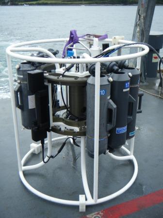
CTD
(a)
 (b)
(b)
 (c)
(c) 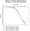
(d)
 (e)
(e)
 (f)
(f)
_small.jpg)
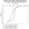
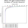
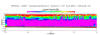
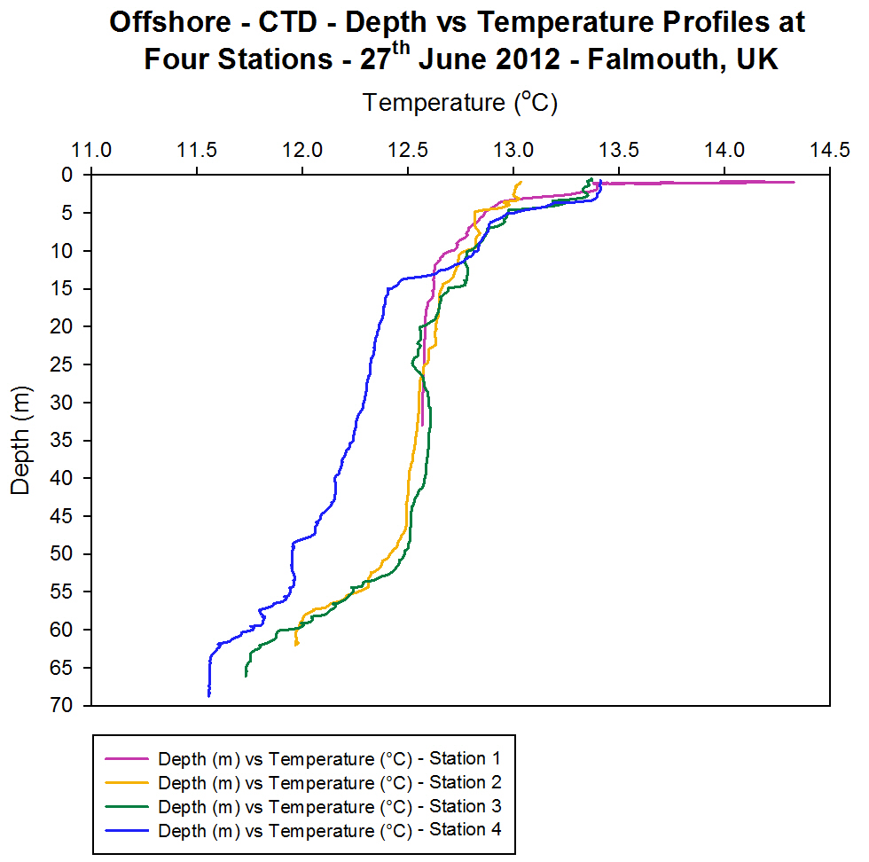
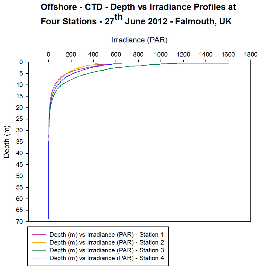
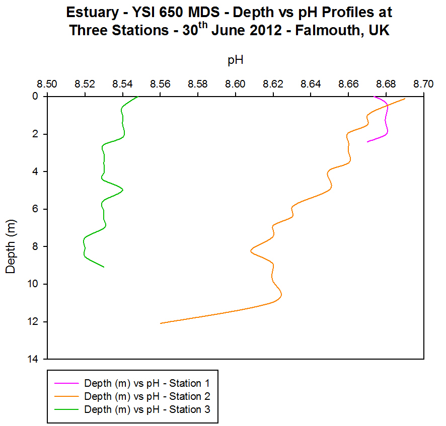
Figure 4.4 - CTD Offshore
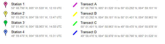
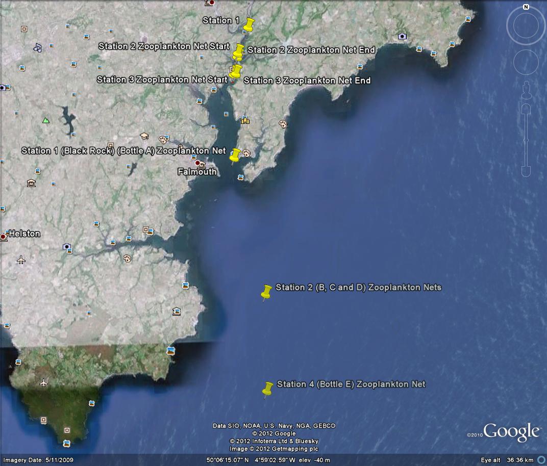
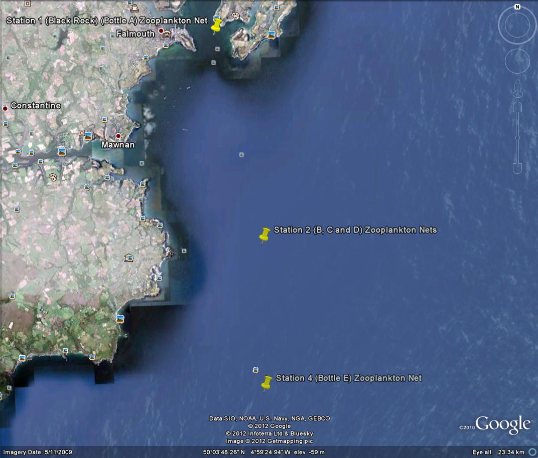
Data collected from Station 1 to Station 4 - Falmouth, UK - (a)
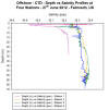
Temperature, (b) Salinity, (c) Density, (d) Fluorescence, (e)
Irradiance, and (f) ln(irradiance). Sampled on 27 June 2012. All
graphs can be enlarged in a new window upon clicking on the relevant
image.
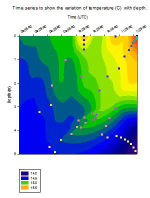
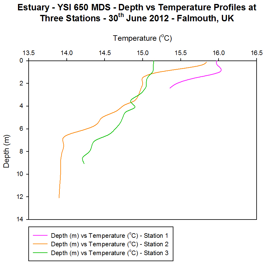
Temperature
[Figure 4.4a]
The vertical
profiles at all stations offshore show a decrease in temperature from
the surface waters to the bottom waters [Figure 4.4a]. At Station 1 the
difference between surface (14.3 ░C) and bottom (12.5 ░C) waters was
approximately 1.8 ░C. The profile at this station showed a rapid
decrease from the surface to 3.5 m, after which the temperature
reduction was observed as more gradual. The rapid change is likely to be
a result of the introduction of warmer, fresher river water flowing
through the estuary to the mouth (where Station 1 was sampled). This
warmer water is at the surface because it has lower density and so is
lighter and floats at the surface. This warmer fresher water can also be
seen in the salinity and density profiles for Station 1 [Figure 4.4b and
Figure 4.4c].
At Station 2
and Station 3 two thermoclines were observed. One from the surface to
approximately 10 m in depth and the other from 47 m to approximately 60
m in depth. The surface thermocline is likely to be a seasonal
thermocline produced due to solar heating of the surface water during
the summer resulting in an increase in the temperature. The difference
in temperature is 0.3 ░C at Station 2 and 0.6 ░C at Station 3. Usually
for this time of year the seasonal thermoclines are stronger with
temperature differences of the order of 2 ░C to 4 ░C (Western Channel
Observatory L4 and E1 buoy data). On the day of sampling, and during
previous weeks of June 2012, the weather had been cloudy and of high
precipitation, thus reducing the amount of incoming short wave radiation
and a reduction in the solar heating of the surface water and so the
thermocline present was weaker. Despite this the presence of this
thermocline indicates that the water column is stratified. The
thermocline present near the bottom of the water column has a
temperature difference of 0.5 ░C at Station 2 and 0.8 ░C at Station 3,
and at this depth could signify the convergence of two water masses at
Station 2 that have different water properties such that one water mass
is downwelling under the other. This idea is further supported by the
presence of a high fluorescence peak at Station 2 at a depth of 49 m
[Figure 4.4d]. Also witnessed at Station 3 was a temperature inversion
at 25 m. This means that the water temperature has increased, in this
case by 0.1 ░C, and could result from mixing between the converging two
water masses seen at Station 2, therefore producing changes to the
properties of the water. This temperature inversion was balanced by an
increase in salinity of 0.05 psu between 25 m and 30 m [Figure 4.4b]
meaning the density at this depth was not significantly changed. Station
4 also shows a thermocline near to the surface decreasing to
approximately 14 m with a temperature difference of 1.0 ░C from 13.4 ░C
to 12.4 ░C. The bottom thermocline is still present at Station 4 but is
less prominent compared to Station 2 and Station 3.
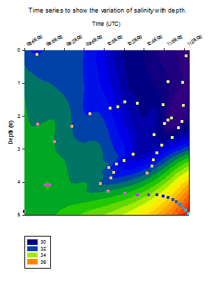
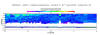
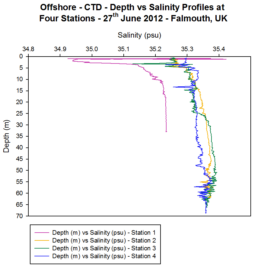
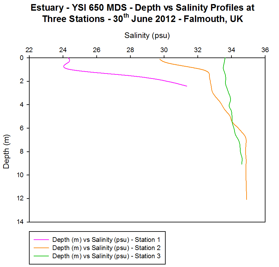
Salinity
[Figure 4.4b]
All four
profiles show an increase in the salinity with depth at Station 1
showing a significant increase and Station 4 a very small increase
[Figure 4.4b]. The stations are positioned at increasing distances from
the shore meaning that the salinity is also increasing from the coast to
offshore as the influence of the higher salinity seawater becomes more
dominant. The lower salinity seen in Station 1 is the result of the
input of warmer and fresher riverine water into the estuary as well as
the high precipitation input experienced in the month of June 2012. This
input of fresher water dilutes the water incoming from the sea thereby
lowering the salinity value of the water and combined with the warmer
temperature mentioned above, the resulting water density is lower
(1026.3 kgm-│).
As mentioned
before there is a more rapid increase in salinity at Station 3 at 25 m
depth coinciding with the temperature inversion at this depth. This
balance prevents the density of the water from changing significantly
and therefore means that no overturning of the water column occurs.
There are
several sharp peaks seen in the vertical salinity profiles in particular
near the surface at Station 1, 3 m at Station 3 and 13 m at Station 4.
These peaks are known as salinity spikes and occur in all CTD profiles
as a result of the time response difference between the conductivity and
temperature sensors on the CTD. They commonly occur in thermocline areas
where the temperature changes are rapid and thus the faster conductivity
response results in a spike in the data.
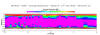
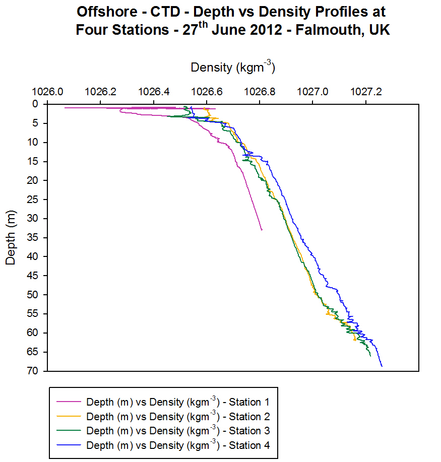
Density
[Figure 4.4c]
At all four
stations the density of the water increases with depth [Figure 4.4c].
This is because density is controlled by the temperature and salinity
characteristics of the water. Water is denser when it is colder and more
saline and from the temperature and salinity graphs the coldest and most
saline water is found at the bottom of the water column and therefore
this is where it has the greatest density. These density profiles show
that the water column at all four stations is statically stable as the
lower density water is on top of the higher density water and no
overturning of the water column is occurring.
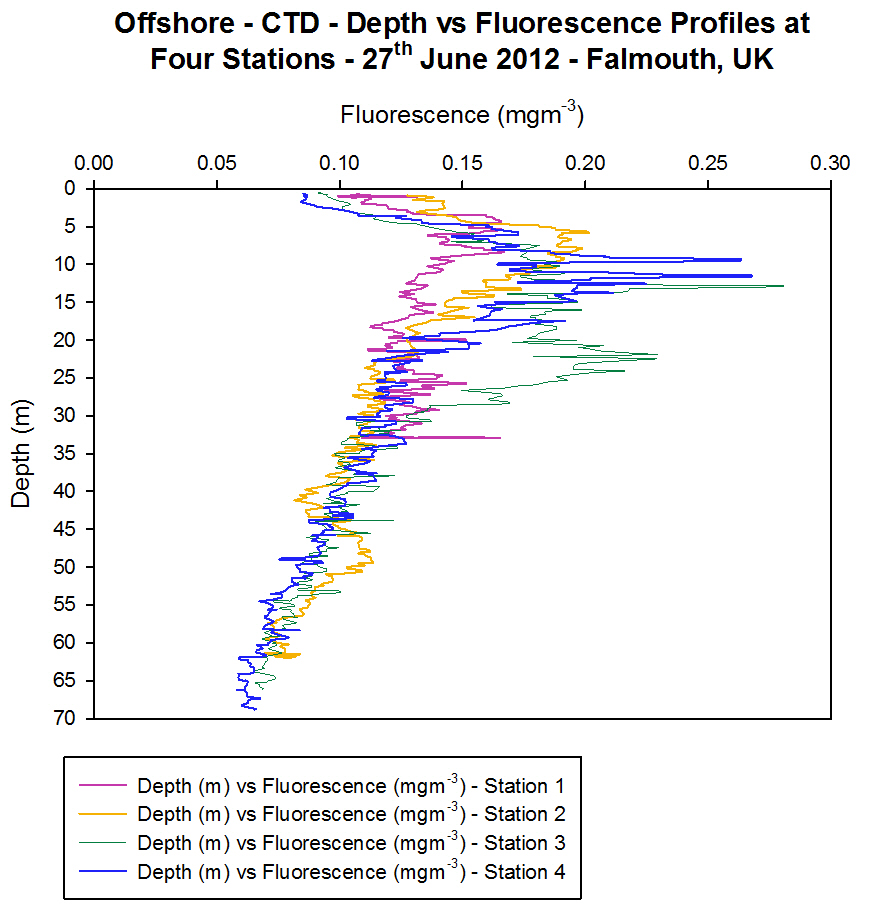
Fluorescence
[Figure 4.4d]
The vertical
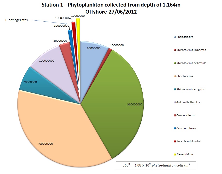
profiles for fluorescence vary with depth [Figure 4.4d]. At Station 1
surface fluorescence values were 0.10 mgm-3 and increased to
a peak value of 0.17 mgm-3 at 4.2 m depth. This peak occurred
due to the chlorophyll pigments present in the sample fluorescing,
signifying the presence of phytoplankton at this depth. This correlates
to the recorded irradiance data, where the euphotic zone at this station
reaches 11 m. This is the level where enough light is available for
phytoplankton to photosynthesise. At Station 2 there were two
fluorescence peaks of 0.2 mgm-3 at 7 m and 0.11 mgm-3
at 49 m. The 7 m peak was due to a chlorophyll maxima resulting from
phytoplankton in the euphotic zone. The peak at 49 m could be a deep
chlorophyll maximum due to the convergence of the two water masses one
of which contained a high chlorophyll concentration/large phytoplankton
numbers and so this downwelling water has subducted the
chlorophyll/plankton also. As the light level is low, it is unlikely
that the phytoplankton are able to photosynthesise at this depth. There
are also fluorescence peaks at Station 3 at depths of 9 m to 11 m (0.26
mgm-3) and at Station 4 at depths of 12 m (0.28 mgm-3)
and 22 m (0.23 mgm-3) respectively. The peak at 22 m at
Station 4 may result from sinking phytoplankton rather than actively
photosynthesising plankton due to irradiance levels of only 10 Ąmolm-▓s-1
which is too low for photosynthesis. The presence of a high number of
zooplankton at this depth supports the theory of a chlorophyll maxima at
this depth since zooplankton feed on phytoplankton. So if a high number
of zooplankton are present then logically one would assume there to be a
food source present to sustain them.
The graph of
chlorophyll against depth derived from acetone extraction [Figure 4.11]
shows peaks of chlorophyll at a similar concentration to that derived
from the fluorometer [Figure 4.4d]. At Station 1, the acetone derived
chlorophyll graph has a peak at 27 m with a value of 5 ĄgL-1.
However the main chlorophyll fluorescence peak from the CTD at 4.2 m is
not seen in the acetone extracted chlorophyll values. At Station 2 the
deeper chlorophyll maxima perceived on the CTD is also seen in the
acetone extracted chlorophyll data where values are 4.4 ĄgL-1
thereby signifying that this is not just an unexpected result from the
CTD only. Station 3 was only a CTD cast so no water bottle samples were
taken and therefore there is no acetone extracted chlorophyll values for
comparison at this station. At Station 4 there is a peak in chlorophyll
extracted from the acetone at 13 m with a value of 5.6 ĄgL-1
which once again coincides with the peak seen by the fluorometer from
the CTD data. This supports the idea that there is likely to by a
chlorophyll maxima at this depth.
When compared
to the chlorophyll data measured by the fluorometer on the CTD the
chlorophyll values extracted from acetone have higher values. The
highest acetone derived chlorophyll value is 5.6 ĄgL-1
whereas the highest chlorophyll concentration from the fluorometer is
0.28 mgm-3. The reason for this difference is due to the
chlorophyll extracted by the acetone measuring all the chlorophyll
present in the water column at that particular depth whereas the
fluorometer only measures the fluorescence by the chlorophyll that have
been excited by the blue light emitted and therefore any other
photosynthetic pigments present that are not excited by the blue light
will not register on the fluorometer. This means that the acetone
extracted chlorophyll values are more representative of the amount of
chlorophyll and therefore more indicative of the concentration of
phytoplankton present in the water column and each of the stations
(chlorophyll concentration is regularly used as a proxy for
phytoplankton concentration, but gives no indication on population size,
as numbers, biomass, and size are all factors).
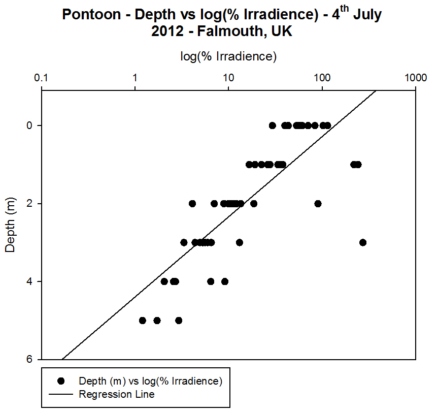
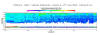
Irradiance
[Figure 4.4e and Figure 4.4f]
For each
station the irradiance profiles show an exponential decrease with depth,
with rapid attenuation of light occurring at shallower depths (between 0
m and 10 m) and slower attenuation occurring below 10 m [Figure 4.4e].
Irradiance decreases exponentially as a result of the attenuation of
light from both absorbance and scattering. Light is absorbed by the
photosynthetic pigments of phytoplankton in the water column as well as
by other particles in the water and the water molecules themselves.
Light can also be scattered by particles in water particularly if high
suspended particulate matter is present. Consequently, the amount of
light reaching greater depths decreases due to these factors. The
surface irradiance values for each station varied from 410 Ąmolm-2s-1
(at Station 1) to 1600 Ąmolm-2s-1
at Station 3. This variation is likely to be as a result of the weather
conditions present (in particular the cloud cover affecting the
irradiance reaching the surface waters). Other factors that affect the
amount of radiation reaching the surface waters are the time of day
which affects the height of zenith, zenith angle, absorption and
scattering in the atmosphere. The 1% value of the surface irradiance can
be used to give an estimate of the depth of the euphotic zone (and so
the depth to which photosynthesis is occurring). At Station 1 the 1%
irradiance value occurs at 11.5 m. At Station 3 the 1% irradiance value
occurs at 8.7 m depth.
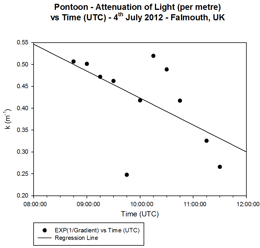
When the
natural log of irradiance is taken the graphs produced closely resemble
straight line relationships (particularly from Station 1). The plots for
the other stations are however not perfect straight lines since other
factors affect light attenuation in the water column. The natural
log of irradiance can be used to calculate the attenuation coefficient
which helps to gain a quantitive value of how much light radiation is
absorbed per metre. The vertical lines at the bottom of the plots are
due to the fact the irradiance values remain consistently low from a
depth of approximately 50 m.
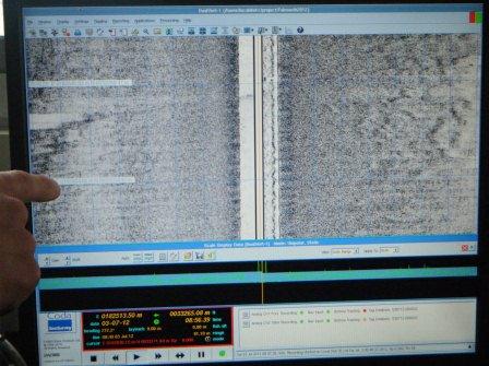
ADCP
(a)
 (b)
(b)
 (c)
(c)
 (d)
(d)
(e)
 (f)
(f)
 (g)
(g)
 (h)
(h)
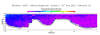
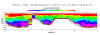
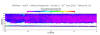
Figure
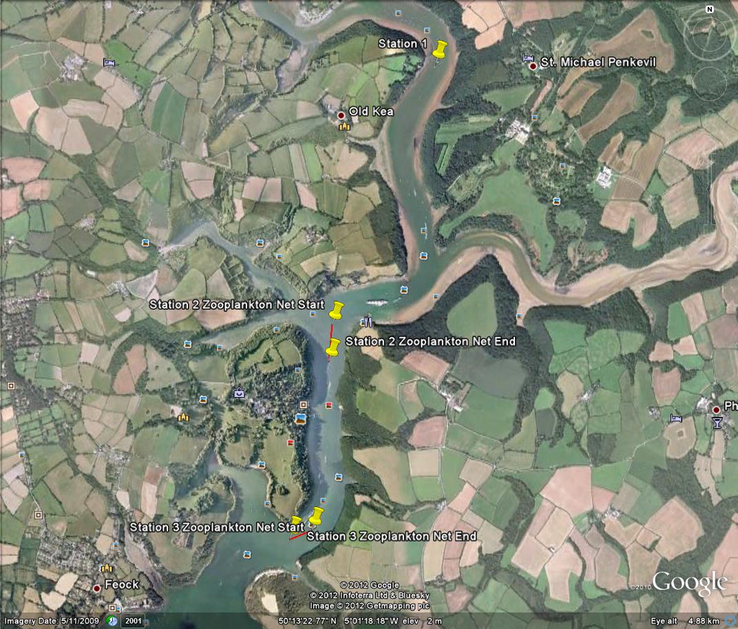
4.5 - ADCP Offshore Data collected from Station 1 to Station 4 -
Falmouth, UK - (a) Velocity magnitude - Station 1, (b) Average
backscatter - Station 1, (c) Velocity magnitude - Station 2, (d) Average
backscatter - Station 2, (e) Velocity magnitude - Station 3, (f) Average
backscatter - Station 3, (g) Velocity magnitude - Station 4, (h) Average
backscatter - Station 4. Sampled on 27 June 2012. All graphs can be
enlarged in a new window upon clicking on the relevant image.
Richardson
Number Graphs:
(a)
 (b)
(b)
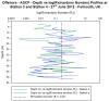
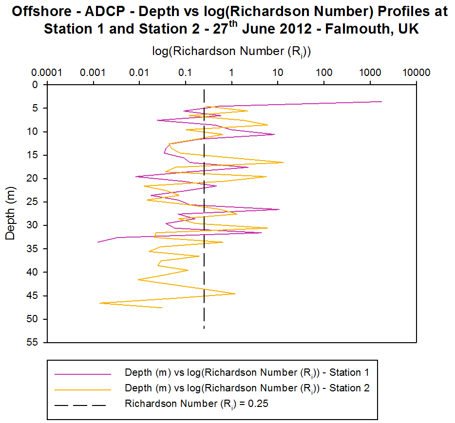
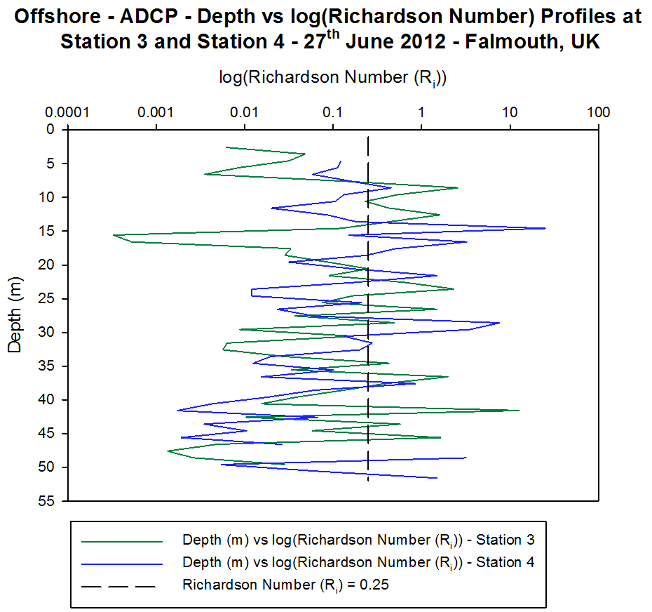
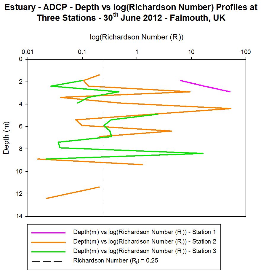
Figure 4.6 - ADCP Offshore
Data of Richardson Numbers (Ri) calculated over a 1 metre
layer (a) Station 1 and Station 2 and (b) Station 3 and Station 4.
Sampled on 27 June 2012. All graphs can be enlarged in a new window upon
clicking on the relevant image.
Station 1 [Figure 4.5a and Figure 4.5b] [Figure
4.6a]
The ADCP profile of velocity magnitude shows
variable velocity in flow with values from slow velocities of 0.011 ms-1
to 0.379 ms-1 with a greater proportion of the flow flowing
at lower velocities at this station. The ship track profile shows that
there is a minimum amount of shear in terms of flow in different
directions but there is shear occurring due to flow at different
velocities. The backscatter data from Station 1 shows very high average
backscatter between 2 m and 10 m depths with values of greater than 80
db. The highest backscatter value recorded at this station was 93 db.
These high values could be produced by zooplankton in the surface water
column but a high backscattering signal can also be the result of
turbulence in the water column.
Between 5 m and 8 m the Richardson number (Ri) is below 0.25
and so the water column at this point is unstable and there is turbulent
flow. This is likely to be a result of the strong winds causing stress
and waves on the surface and below the surface of the water. High water
was at 10:20 UTC on this day, so the turbulent flow may also have been
as a result of the ebbing tide. From 8 m to 11 m and 16 m to 19 m the
Richardson number is above 0.25 and therefore flow is stable and laminar
so the high backscatter values of 76 db to 78 db between 10 m and 20 m
is more likely to be produced by zooplankton with some backscatter
resulting from the turbulent flow at 11 m to 16 m. Except for 25 m to 27
m and 30 m to 32 m the rest of the water column exhibits turbulent flow
[Figure 4.6a].
Station 2
[Figure 4.5c and Figure 4.5d] [Figure 4.6a]
The ADCP profile of velocity magnitude also shows
variable velocity in flow at Station 2 with values from slow velocities
of 0.005 ms-1 to high velocities of 0.614 ms-1
with a greater proportion of the flow flowing at lower velocities at
this station. The ship track profiles show that at the shallower depths
(2 m to 5 m) and the deeper depths (39 m to 48 m) of the water column
there is significant shear occurring with flow travelling in different
directions and at different velocities relative to one another.
The backscatter data from Station 2 also shows very
high backscatter between 2 m and 10 m depths with values of greater than
80 db and high backscatter (values above 70 db) up to 20 m depths
[Figure 4.5d]. The highest backscatter value recorded at this station is
106 db. Due to the waves created by the weather the very high
backscatter is likely to be created by these whereas the high values
lower down is more likely to be created by zooplankton. The surface
waters of Station 2 have values above 0.25 with a Richardson number high
of 8.5. This shows that the waters are laminar which coincides with the
presence of the thermocline at the surface creating stratification and
the laminar flow. Below 34 m to 44 m the Richardson number is lower than
0.25 which may be to do with the mixing occurring between the two
converging water masses creating small scale turbulence. The second
thermocline seen at Station 2 has formed a small laminar flow layer at
45 m where the Richardson number is above 0.25 (Ri
= 1.17) [Figure 4.6a].
Station 3 [Figure 4.5e and Figure 4.5f] [Figure 4.6b]
The ADCP profile of velocity magnitude at Station 3
shows higher velocity flow than at Stations 1 and 2 with values from
0.195 ms-1 to 0.673 ms-1. The ship track profiles
show that at the shallower depths (2 m to 10 m) of the water column
there is significant shear occurring with flow travelling in different
directions and at different velocities relative to one another but below
15 m the direction of flow is relatively constant (approximately 215░)
[Figure 4.5e].
For a large proportion of the water column at
Station 3 the backscatter is low with values of 63 db to 68 db with only
a thin layer of water at the surface exhibiting large backscatter. Once
again due to the weather this is likely to be the result of wind and
wave mixing causing scattering of the sound emitted from the ADCP. This
weather affect is seen in the Richardson number graph where the surface
waters have a Richardson number below 0.25 representing turbulent flow
at which point the water column has instability [Figure 4.6b]. The
Richardson numbers with depth at Station 3 are below 0.25 for the
majority of the water column except at 7.5 m to 13.7 m, 21 m to 27 m and
40 m to 46 m where the Richardson numbers are 2.67, 2.29 and 12.2
respectively, indicating that at these depths the flow is stable and
laminar.
Station 4 [Figure 4.5g and Figure 4.5h] [Figure 4.6a]
The
ADCP profile of velocity magnitude at Station 4 also shows higher
velocity flow than at Station 1 and Station 2 with values from 0.087 ms-1
to 0.946 ms-1. The ship track profiles show that at the
shallower depths (2 m to 10 m) and the deeper depths (43 m to 50 m) of
the water column there is significant shear occurring with flow
travelling in different directions and at different velocities relative
to one another but below 12 m the direction of flow is relatively
constant (approximately 235░) [Figure 4.5g].
Similar to Station 3 the average backscatter for a
large proportion of the water column at Station 4 is low with values of
64 db to 70 db. There is an area at the surface with very high
backscatter (115 db) which is likely caused by turbulence which is shown
from the Richardson number graph with values below 0.25. The relatively
high backscatter (76 db) in the top left of the backscatter contour
could be related to high zooplankton numbers in this layer scattering
the sound. This explanation is more likely particularly at depths of 13
m to 18 m where the Richardson number is above 0.25 and so the flow is
laminar and the water column stable - thus not likely to be scattering
the sound.
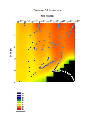
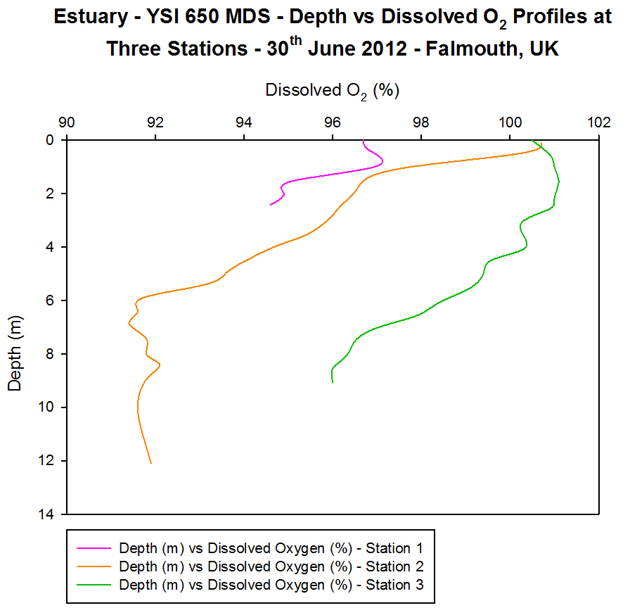
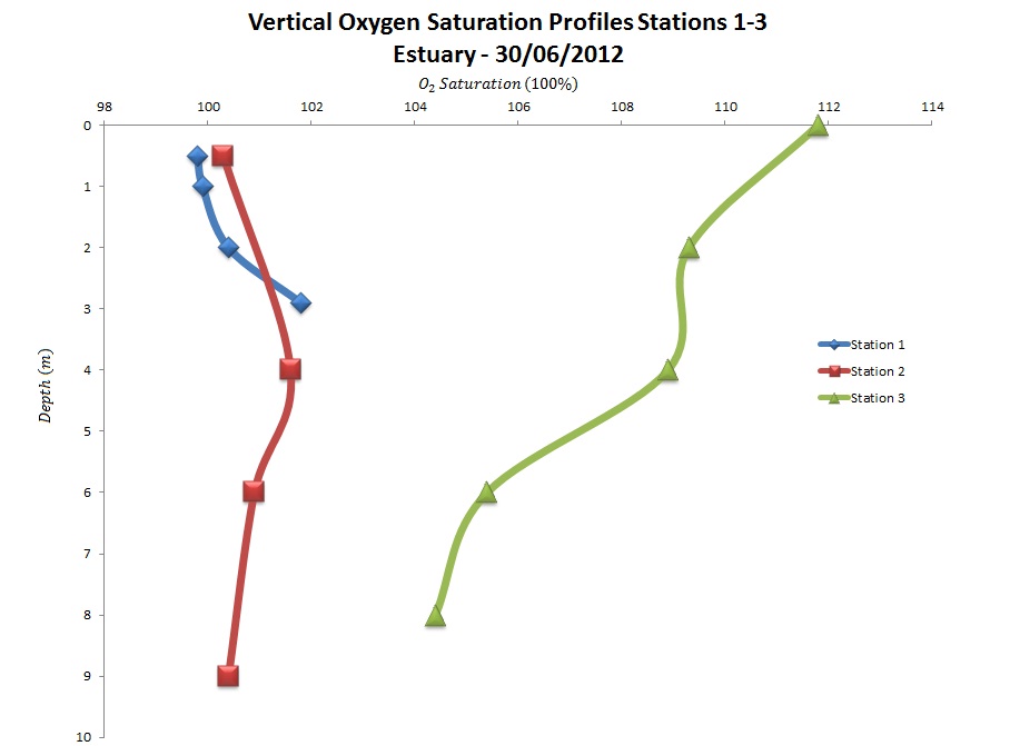
Dissolved Oxygen
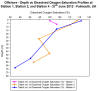
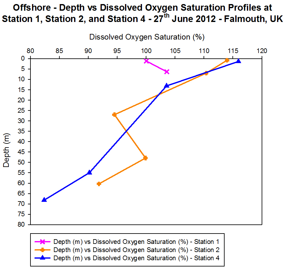
Figure
4.7 - Offshore dissolved oxygen saturation. Sampled on 27 June 2012.
Graph can be enlarged in a new window upon clicking on the relevant
image.
The samples from Station 1 show percentage of dissolved oxygen (%O2)
saturation increased from a depth of 1.16 m where saturation was 100.0%
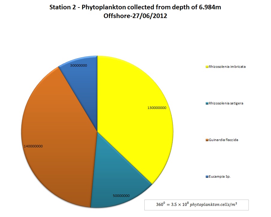
to 6.30 m where saturation was at 103.6%. Station 2 and Station 4
generally showed a decrease in %O2 saturation with depth. The
decrease in %O2 saturation at Station 2 between the depths
0.80 m and 6.98 m with 3.6% with %O2
saturation values of 114.0% and 110.4% respectively (decreased at a rate
of 0.58% m-1 depth). There was also a 3.6% decrease between
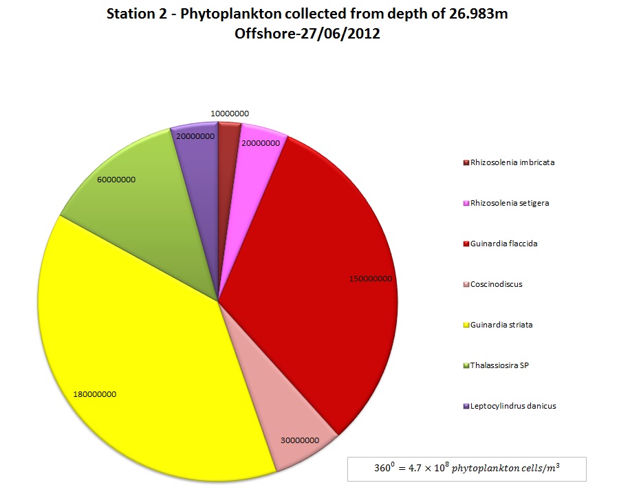
the depths 6.98 m and 26.98 m with %O2 saturation values of
110.4% and 94.5% respectively (decreased at a rate of 0.79% m-1
depth), which was slightly more gradual than at Station 4. At depths of
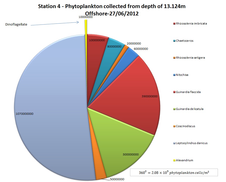
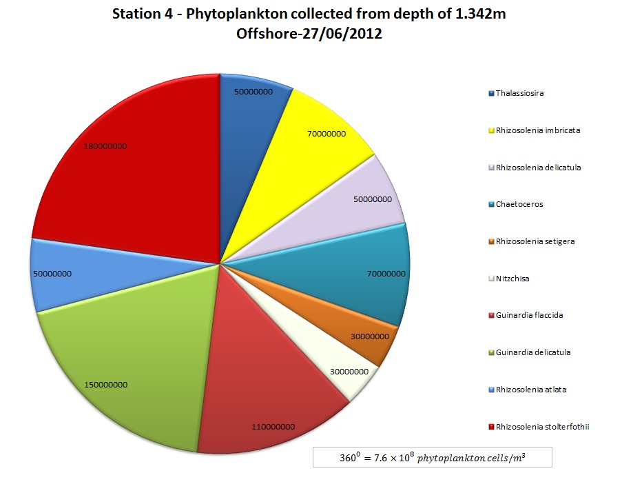
1.34m and 13.12m Station 4 showed higher %O2 saturation
values of 115.96% and 103.53% respectively (decreased at a rate 1.06% m-1
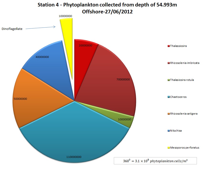
depth). Between the depths of 13.12m and 54.99m, Station 4 showed
a more gradual rate of decrease in %O2 saturation with depth
(0.32% m-1
depth) when compared with Station 2 (0.79% m-1 depth).
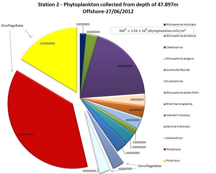
Station 2 showed a slight spike in %O2 saturation between a
depth of 26.983m and 47.897m from 94.5% to 99.9% (5.37% increase) after
which %O2 saturation gradually decreased again with depth.
Station 2 and Station 4 showed much higher surface %O2
saturation (114.0% and 115.96% respectively) than that of Station 1
(100.00%).
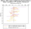
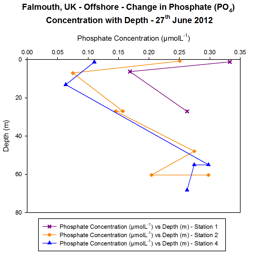
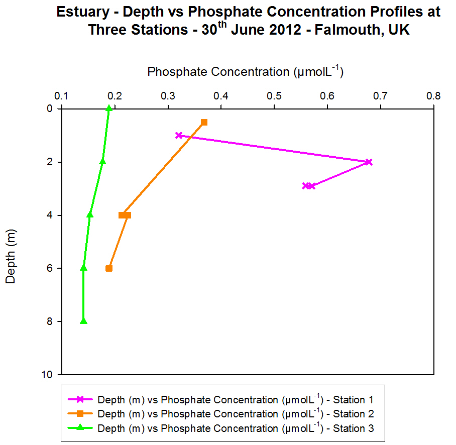
Phosphate
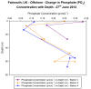
Figure 4.8 - Offshore dissolved phosphate concentration. Sampled on 27
June 2012. Graph can be enlarged in a new window upon clicking on the
relevant image.
During the offshore investigation into phosphate concentrations Niskin
Bottles were used to collect water samples at three stations. The
samples were places in a spectrophotometer to analyse, this piece of
equipment had a detection limit of 0.03
ĄmolL-1
for phosphate. From this data it was found that Station 1 had a high
surface phosphate concentration of 0.333 μmolL-1
which decreased to 0.169 μmolL-1 by 6 m depth; this is the
minimum which then rises again at 25 m.
These lower values correspond to the fluorescence peak observed on the
CTD data which could be an indication of a chlorophyll maximum. The
increased chlorophyll levels may be linked to an abundance of
phytoplankton at a depth of 6 m, whereas they are not present in the
same abundance at depth so phosphate concentrations increase again.
At Station 2 two thermoclines were observed along with a chlorophyll
maximum at these depths. The phosphate data corresponds with this
maximum, with a high value at the surface which again decreases at 6 m
the same as Station 1; however the lowest value observed here is 0.075
μmolL-1 compared with 0.169 μmolL-1
at the previous site showing it has been removed more in this area than
at Station 1 sampling site.
By 27 m this concentration has dropped to 0.157 μmolL-1 but
increases to 0.274 μmolL-1 by 47.9 m as it is being used
less at this depth compared to nearer to the surface where there is more
biological activity occurring. At 60 m depth two bottle samples were
taken showing both a decrease to 0.204 μmolL-1
and an increase to 0.298 μmolL-1 at the same site which
could be due to them sitting on slightly different positions along the
CTD rosette.
Station 4 also showed the thermocline was still present, here five
bottles were fired on the CTD showing very low concentrations of
phosphate just under the surface waters at only 0.110 μmolL-1,
and this lowered even further by 13 m. No further readings were taken
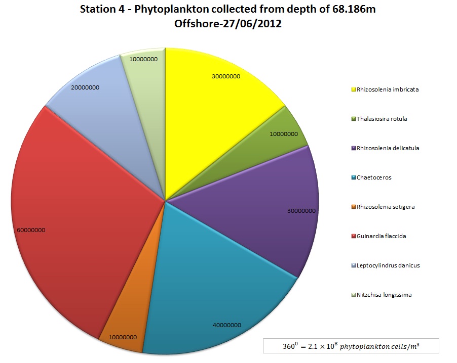
until 55 m depth where the concentration was found to be 0.298 μmolL-1
and it remained around this figure at the next sample depth of 68 m.
This drop in concentration may again link to the maximum reading shown
by the fluorometer during the investigation at this station.
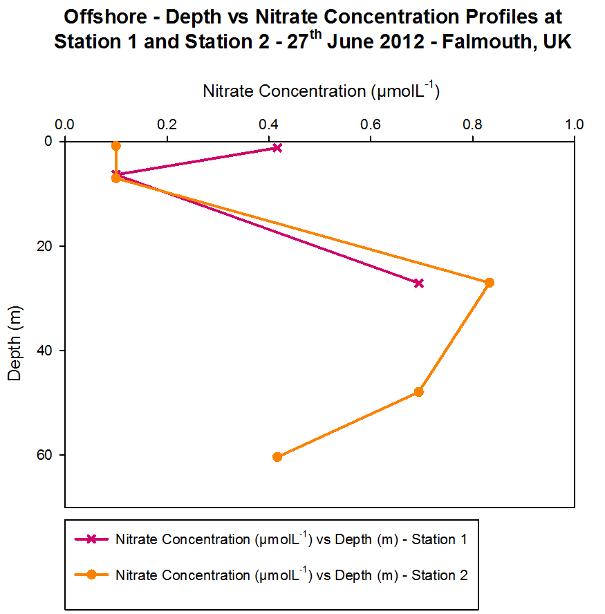
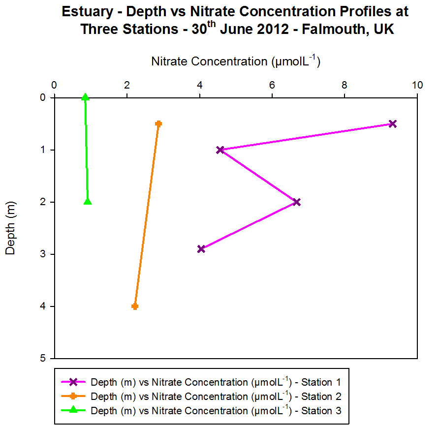
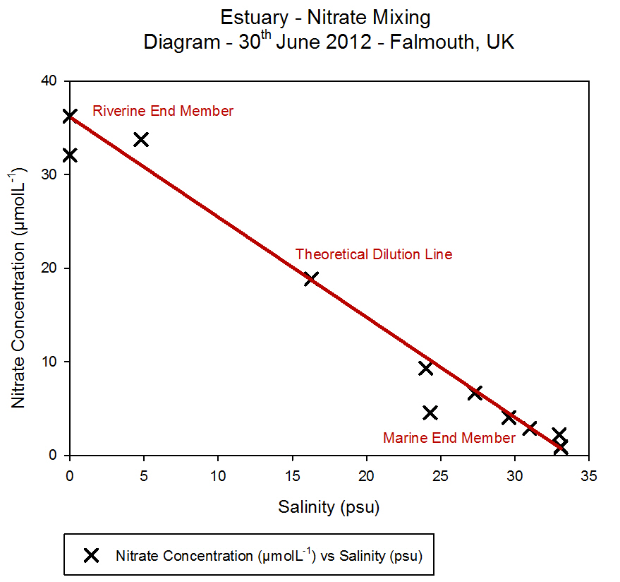
Nitrate
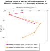
Figure 4.9
- Offshore dissolved phosphate concentration. Sampled on
27 June 2012. Graph can be enlarged in a new window upon
clicking on the relevant image.
The nitrate data shows a vertical profile for Station 1 and Station
2. Nitrate is an important macronutrient in phytoplankton growth; it is
generally considered to be the limiting nutrient for plant growth in the
sea. Nitrate is taken up by phytoplankton and reduced to ammonium so it
can be incorporated into carbon skeletons. Therefore, it was
hypothesised that when there was a low nitrate concentration, this may
correlate with a peak in fluorescence on the CTD data as fluorescence is
indicative of the presence of phytoplankton.
At Station 1, the nitrate concentration was 0.417 ĄmolL-1
in the surface sample, then decreases to a level that was undetectable
by the flow injection analysis, due to removal by phytoplankton. The
detection limit for the equipment used was 0.1 ĄmolL-1,
meaning that if the concentration was less than 0.1 ĄmolL-1,
then this was plotted on the graph as 0.09 to show that it was below
this value. The maximum nitrate concentration was measured at 27 m, and
here the fluorescence levels were low, indicating low phytoplankton
presence to utilise the nitrate.
At Station 2, the nitrate levels were undetectable in approximately the
top 6 m of water. This minima correlates with the fluorescence peak in
the CTD data of nitrate concentration was greatest, where small peaks
can be seen at approximately 4 m, 6 m and 8 m. The maximum nitrate
concentration is seen when the fluorescence drops to 0.10
mgm-3,
as there are fewer phytoplankton to cause removal of nitrate from the
water column.
The two main sources of nitrogen in the euphotic zone are either
regenerated e.g. bacterial oxidation to nitrate by the benthic
decomposition of organic matter (Kemp et al., 1988) below the
thermocline replenishes surface waters with nitrate, or new nitrogen
e.g. imported from the deep ocean or the atmosphere in the form of
ammonium or urea. Phytoplankton can only take up regenerated forms
of nitrogen such as nitrate, which is why removal is seen in correlation
with peaks in chlorophyll.
Other possible influences on nitrate levels could be from terrestrial
origins that have washed into the estuary and entered the area
offshore. The rainy weather conditions recently could have increased the
amount of runoff occurring and therefore raised the nitrate levels. This
would have particularly affected Station 1 which was located at the
mouth of the estuary as this is closest to any terrestrial sources, and
has a higher surface concentration of nitrate than Station 2 which was
further offshore.
In reality there would be much more variation in nitrate concentration
through the water column, but as the number of water samples that could
be collected and processed was limited, the data only shows a snapshot
of the vertical variations and not a continuous profile.
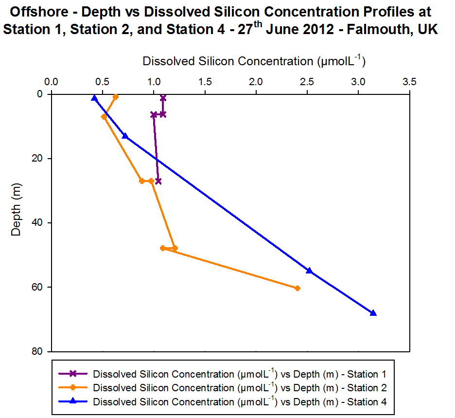
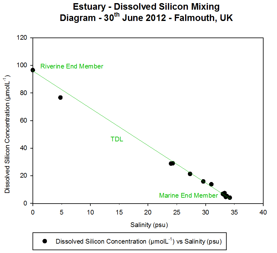
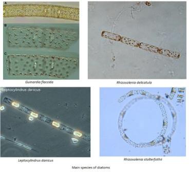
Dissolved Silicon
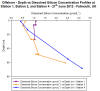
Figure 4.10 - Offshore
dissolved silicon concentration. Sampled on 27 June 2012. Graph can be
enlarged in a new window upon clicking on the relevant image.
Dissolved silicon is present in seawater within
silicate, SiO44-. It is utilised within the
frustules of diatoms as a structural component, with diatoms accounting
for 90% of suspended dissolved silicon in the world's oceans (Harper.,
1975). It is also important in other siliceous phytoplankton, such as
dinoflagellates. As such, dissolved silicon concentration is an
indicator for phytoplankton presence, and vice versa.
At Station 1, the dissolved silicon concentration
was almost constant with depth. Over the 20 m sample depth range, there
was a decrease of only 0.1 ĄmolL»╣, from 1.1 ĄmolL»╣ at 1.2 m to 1.0
ĄmolL»╣ at 27.0 m. The replicate analyses of the 6.3 m had a difference
of 0.1 ĄmolL»╣ between them, suggesting that the method of analysis was
precise. At Station 2, the dissolved silicon concentration increased
with depth. There was an overall difference in dissolved silicon
concentration of 1.9 ĄmolL»╣ over the 60 m depth range. The highest
concentration was 2.4 ĄmolL»╣ at 60.4 m. The two sets of replicates
analysed from water sample taken at 27.0 m and 47.9 m both had a
difference of 0.1 ĄmolL»╣ between them, suggesting that the method of
analysis was precise.
At Station 4, the dissolved silicon concentration
increased with depth. There was an overall difference in dissolved
silicon concentration of 2.7 ĄmolL»╣ over the 67 m depth range. The
highest concentration was 3.1 ĄmolL»╣ at 68.2 m.
In general, there was an exponential increase in
the dissolved silicon concentration with increased depth. The nearest
sample taken to the surface at each station decreased in dissolved
silicon concentration as the stations moved further offshore.
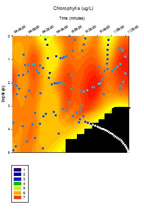
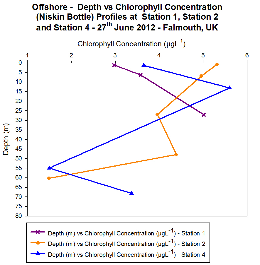
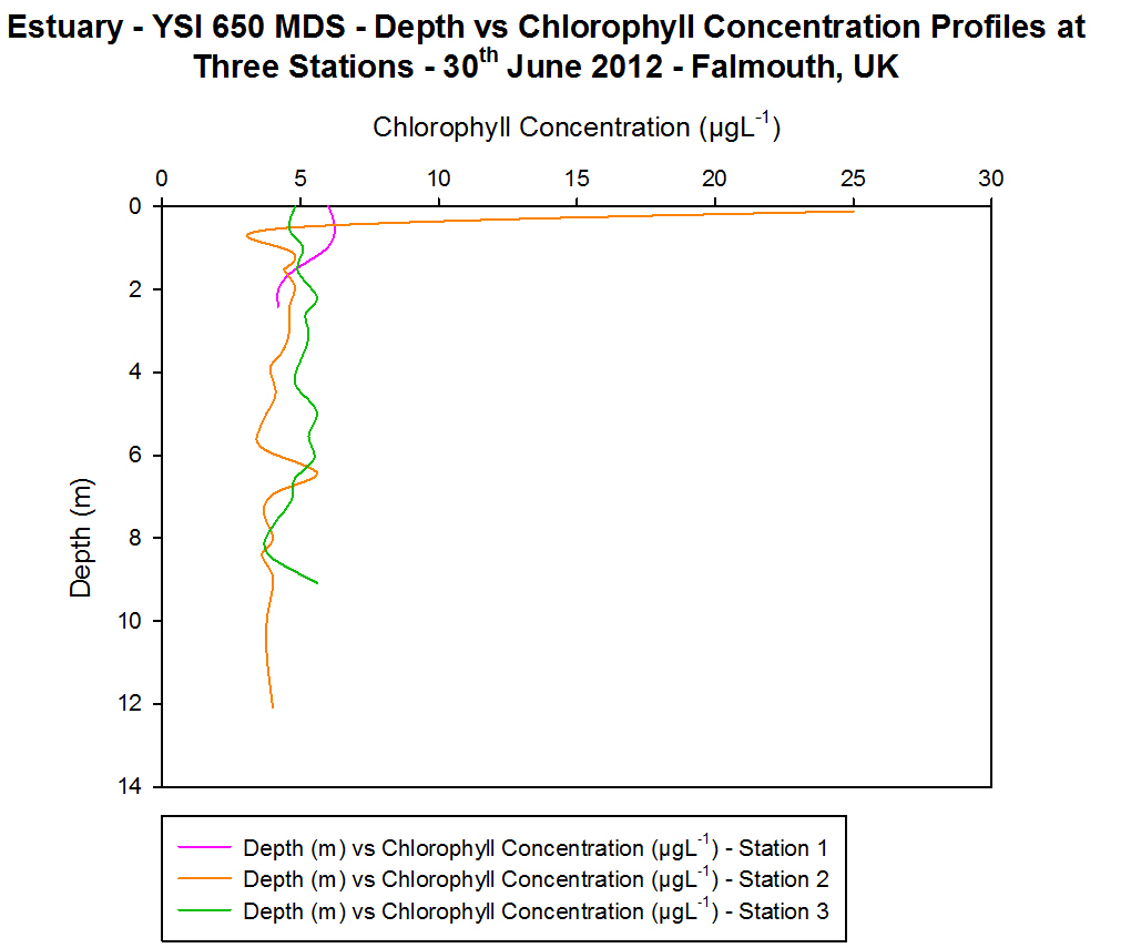
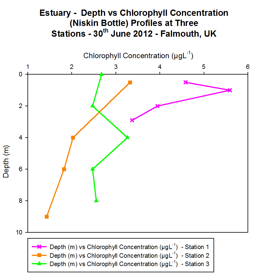
Chlorophyll
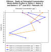
Figure 4.11 - Offshore
chlorophyll concentration (Niskin bottle). Sampled on 27 June 2012.
Graph can be enlarged in a new window upon clicking on the relevant
image.
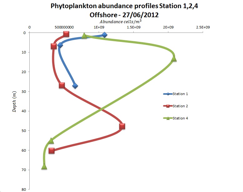
For surface waters the highest chlorophyll
concentrations are found to be at Station 2 (> 5 ĄgL-1). The
lowest surface chlorophyll concentrations can be found at Station 1
(Black Rock) (< 3 ĄgL-1) and intermediate chlorophyll
concentration values are located at Station 4 (approximately 3.6 ĄgL-1).
Down to a depth of 28 m chlorophyll concentration at Station 1 continues
to increase but at this depth no more samples are taken and it peaks at
approximately 5 ĄgL-1. Chlorophyll concentration at Station 4
peaks at 15 m depth where it reaches concentrations > 5.5 ĄgL-1.
Further down in the water column at approximately 55 m depth the
concentration had dropped to approximately 1. 5 ĄgL-1 which
was the joint lowest concentration measured in the offshore practical.
Between 55 m and 70 m the chlorophyll concentration increased again to
above 3 ĄgL-1 and sampling did not continue at any greater
depths. At Station 2 the highest chlorophyll concentrations are found at
the surface and they generally decrease with depth until the lowest
concentration is found at 60 m (approximately 1.5 ĄgL-1).
(a)
 (b)
(b) 
(c) 


.jpg)


 (b)
(b)  (c)
(c) 
 (e)
(e) 


 (b)
(b)
 (d)
(d)
 (e)
(e)