-Group 7-
Investigators: Claire Critchley, Oscar Dunn, Kelly Edwards, Christian Laurent, Ben Lawn, Harriet McGrain, Fiona Roffey, Brendan Selkirk, Mike Wood and Henry Yu.
 Group
7 carried out an oceanographic investigation looking at coastal,
estuarine and offshore variables in and around the Fal estuary,
Cornwall, UK from 25th June to 6th July 2012.
Group
7 carried out an oceanographic investigation looking at coastal,
estuarine and offshore variables in and around the Fal estuary,
Cornwall, UK from 25th June to 6th July 2012.
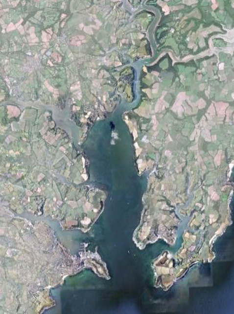
The Fal estuary is England’s largest estuary, extending 18km inland. It is important for trade, tourism and conservation (Langston et al., 2003). The Fal estuary is a ria; formed when the sea level rose at the end of the last Ice Age (Langston et al., 2006). Thus, the Fal estuary has a low freshwater input and a large diversity of marine habitats. The estuary is macrotidal at Falmouth, and it becomes mesotidal at Truro, with mean spring tidal range of 4.6m and 3.5m respectively (UKHO,2008). There are extensive wetlands in both the upper Fal and the lower Fal, which is the third largest natural harbour in the world (Pirrie et al., 1995).
The Fal estuary is a Site of Special Scientific Interest and a Special Area of Conservation due to the variety of abundant habitats which include intertidal mudflats and sandflats, sub-tidal sandbacks, eelgrass beds, maerl beds on St Mawes Bank and maerl gravel scattered throughout the estuary. The maerl beds are the largest in South West England and there are a wide variety of epifaunal and infaunal species including the rare Couch’s goby Gobius couchi (Langston et al., 2003). The Fal estuary is also classified as a Sensitive Area (Eutrophic) as it has a high risk of hypernutrification and eutrophication throughout the estuary in summer. (Maier et al., 2008).
The catchment and the sediments are affected by mineralisation. The local geology consists of Carnmellis granite and metamorphic aureole and these greatly influence the current synthesis, particularly in the rivers which also have acid-mine drainage (Hosking and Obial, 1966). Mining of metalliferous deposits has occurred since the Bronze Age. Most of the remobilised metal and tailings from the mining activity was deposited in Restronguet Creek. Today, metal contamination in the Restronguet sediments remain the highest in the UK for some metals including copper, zinc, iron, tin, arsenic and manganese (Bryan and Langston, 1992). The last mine, the Wheal Jane, was abandoned in 1991, although there is still china clay quarrying in the St Austell area causing major silting in the upper Fal estuary and saltmarshes.
Current anthropogenic impacts include direct point source discharges from boats, agricultural run-off, sewage from the local towns and there are issues with invasive species being transported through ballast water due to the busy port and large recreational marinas . Historic anthropogenic impacts for the last century are still impacting upon the present marine environment through high metal contamination and an increase in tri-butyl tin concentration from anti-fouling paint used on the hulls of the boat.
![]()
![]()
![]()
![]()
|
|
YSI Probe: 6600v2: a 6-series multiparameter sonde made by YSIinc.
|
 |
|
LI-COR Light Probes LI-210 photometric surface sensor by LI-COR Environmentalinc, and LI-192 underwater quantum sensor, also by LI-COR. The surface sensor is used to record the incoming light intensity at the water surface, and the underwater sensor used to measure light intensity at varying depths. The comparison of the two readings allow calculation of a light attenuation coefficient, k.
|
 |
 |
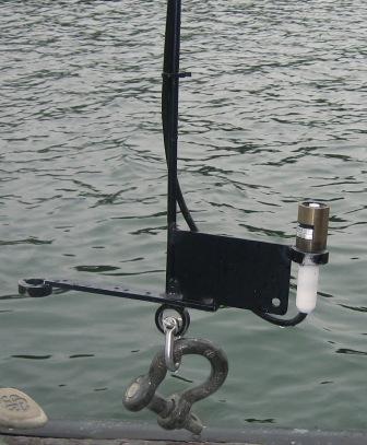
Valeport current meter Model 106 Lightweight analogue current meter by Valeportltd. Current velocity is measured using the impeller and the flux gate compass records the direction of flow.
|
![]()
![]()
![]()
![]()
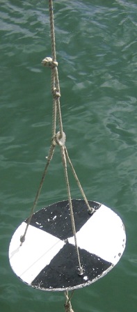 |
Secci Disk A circular weighted disk divided into alternating black and white quadrants which is lowered through the water column to a point where the disk is no longer visible to the human eye. The 1% light depth is 3 times the rope lowered.
|
|
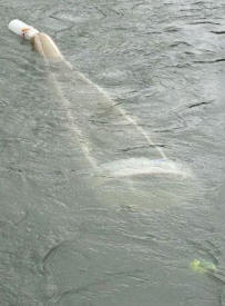
Plankton Net A cone shaped net which is connected to a sampling bottle and deployed off the stern at low speeds to trap phytoplankton and zooplankton. It was manually controlled using a rope to maintain net position just below the surface so that a representative sample may be collected. The net has a 50cm diameter aperture and a mesh size of 210µm which had an approximate entrance area of 0.196m2. The water volume that passed through was calculated from an impellor suspended in the net with a 5 digit counter. Each revolution equals 0.3m. |
 |
 |
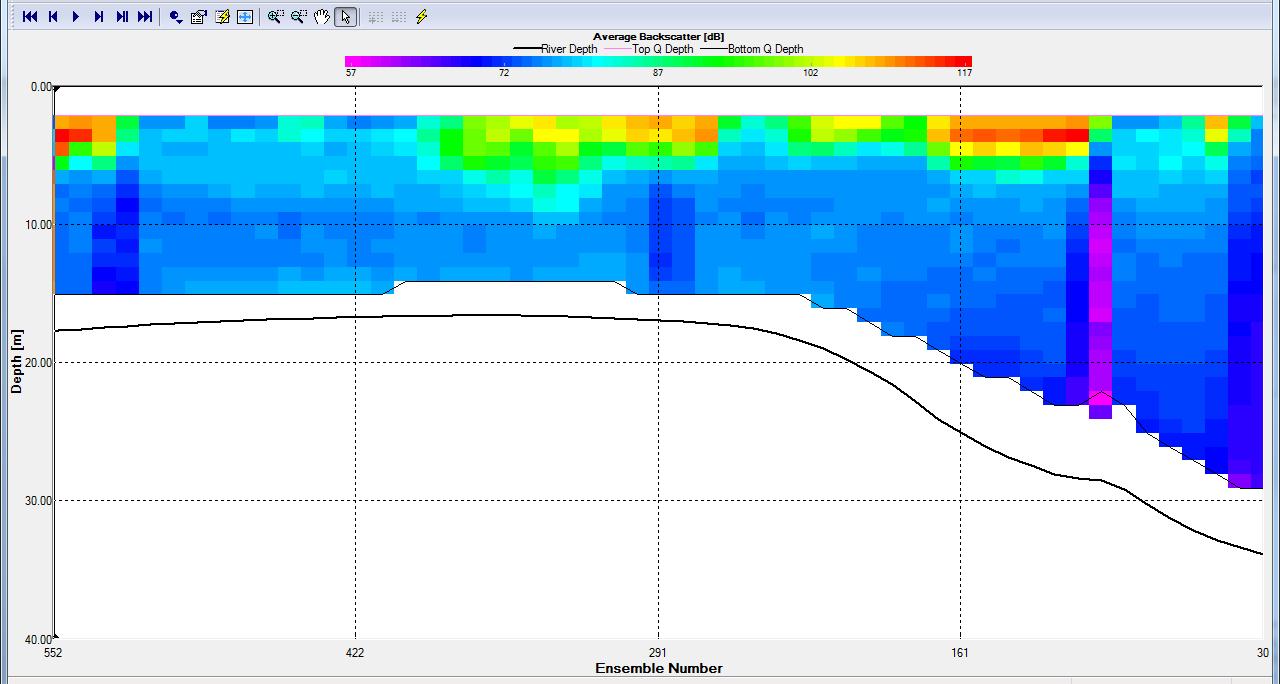
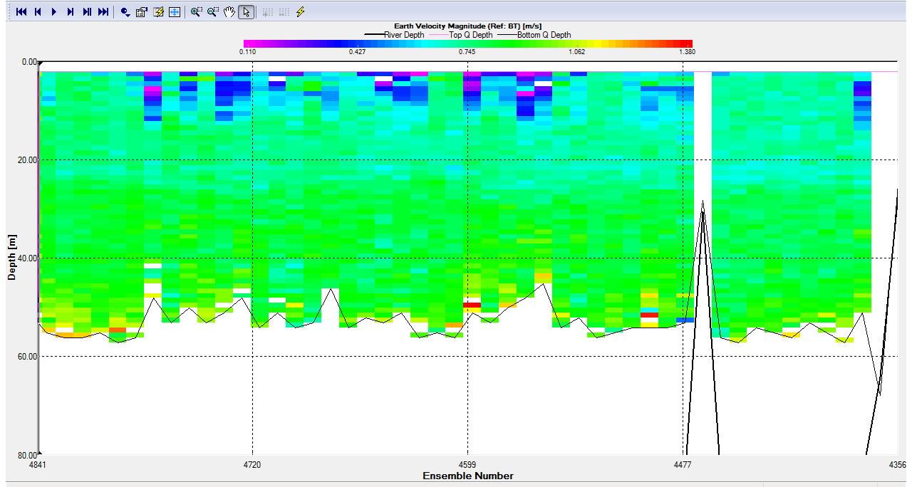
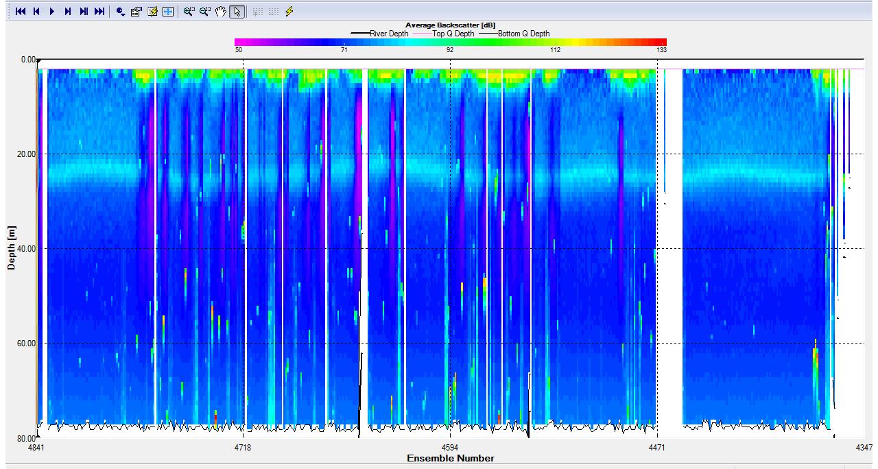
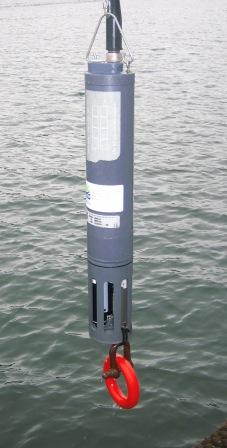
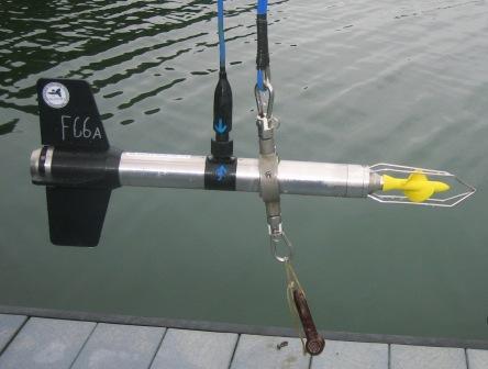
ADCP An Acoustic Doppler Current Profiler is attached to the hull of most research vessels. It measures current flow velocities along transects by using Doppler Shift. There are four transducers, in the x, y and z direction with a fourth used as a control and back up. The transducers send a pulse of sound and then receive it at a different frequency. Particles which are moving towards the receiver will produce a higher frequency and particles which are moving away from the receiver will produce a lower frequency. The ADCP takes into account the movement of the vessel and can be used to detect backscatter, indicating areas which contain a high abundance of Zooplankton.. The ADCP on the Bill Conway is 1200kHz and had a 5cm vertical resolution, magnetic flux gate compass producing latitude and longitude co-ordinates and its clock is precise to 0.01 seconds. |
|
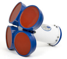
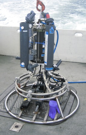
CTD The Conductivity, Temperature and Depth probe is used to record vertical profiles of temperature, salinity and depth based on pressure. Most CTD’s are attached to a Rosette system along with Niskin bottles, this enables additional parameters such as turbidity, dissolved oxygen and nutrient concentrations to be measured at discrete depths via water sampling. The CTD is connected to the boat using a conductive cable enabling control over its depth and the controlled closure of the Niskin bottles.
|
 |
![]()
![]()
![]()
![]()
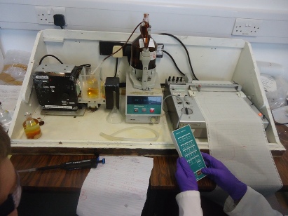 |
Dissolved oxygen analysis Approximately a 120ml sample of the water collected in the niskin bottles was drawn into separate bottles where 1ml of manganous sulphate and 1ml of alkali-iodide-azide was added to them forming a precipitate which preserved the dissolved oxygen contained in the sample. These samples were analysed using the Winkler Titration method. This involved firstly adding 1ml of sulphuric acid to each of the oxygen samples which dissolved the precipitate, before mixing the sample with Thiosulphate solution (normality: 0.22) to determine the dissolved oxygen percentage. |
|
Chl a determination 50ml water samples from the Niskin bottles had been syringed through a 0.7µm glass fibre filter, and the filter chilled in 6ml of Acetone overnight. The spectrophotometer was zeroed with a clean empty tube, before each sample was transferred to a glass test tube for analysis in the spectrophotometer. Fluorescence readings were converted into µg/l using the following equation.
|
 |
|
By measuring the fluorescence of chlorophyll dissolved in acetone in response to a set wavelength the chlorophyll concentration can be calculated by use of a standardised calibration curve. 10 AU Field Fluorometer Specifications Detection Limit for Chlorophyll: 0.025µg/L using EPA method 445.0 Linear range for extracted chlorophyll α: 0-250µg/L Electrical Specifications: 4 watts, 8000 hours lamp life Detector: PhotoMultiplier Tube; 300-650nm, red 185-870nm |
|
Phosphate concentration analysis The mixed reagent was composed of 20% Ammonium Molybdate, 50% Sulphuric acid (2.5M), 20% Ascorbic acid and 10% Potassium antimonyl tartate. The mixed reagent was made using a measuring cylinder, washed with MQ water before the addition of different chemicals. Surplus mixed reagent was made to ensure there were sufficient quantities for all samples and standards. A 400-fold dilution of the standard stock solution was required for the makeup of the standards. 1ml of the stock standard was transferred into a 100ml volumetric flask using a hand pipette and made up to 100ml with MQ water. 25ml of this solution was transferred into another 100ml volumetric flask and further diluted by making up 100ml with MQ water. Three empty bottles were filled with 10ml of MQ water and these were used as blanks. 50 µl, 100 µl, 200 µl, 500 µl, 1000 µl, 2000 µl and 4000 µl were hand pipetted into separate empty bottles and 1ml of mixed reagent was added, this was left for an hour to react. For each individual standard of known PO4 concentration, three replicates were made to reduce the effects of error. Simultaneously, 10ml of the individual samples were transferred to individual bottles where 1ml of the mixed reagent was added and given an hour to react. Then, all the standards and samples were analysed using the U-1800 Spectrophotometer at 882nm with cell size of 4cm.
|
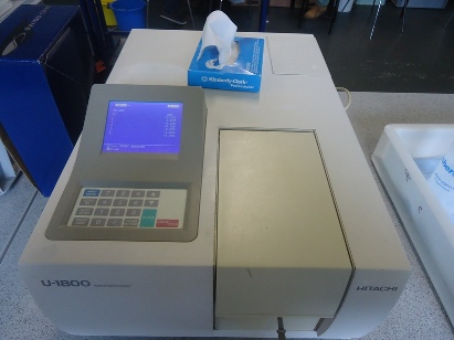 |
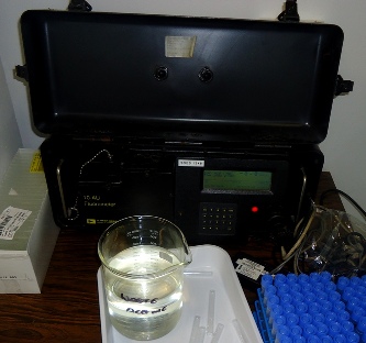
Hitachi spectrophotometer U-1800 The spectrophotometer was used to quantify the levels of phosphate and silicon present in the collected samples, by measuring absorbance of the samples at specific wavelengths and using calibration standards to calculate a nutrient concentration value.
|
|
Silicon Analysis The method is adapted from Strickland and Parsons (1968). The blanks allow corrections for any input of silica from the equipment or the reagents. A silicomolybdate complex was formed and reduced by metol and oxalic acid to produce a blue solution with an extinction coefficient at 810nm wavelength, which was proportional to the colour’s intensity. A stock of 35.6mol of silicon concentration was diluted 25 times to produce the working stock of silicon concentration used in all samples. The standards were made up to contain set silicon concentrations using the concentrations below. |
|||||||||||||||
|
|||||||||||||||
|
The same procedure was used to measure the standards. 5ml of sampled water or MQ water in the case of the standards was added to each polypropylene tube. 2ml of molybdate solution was added to each sample, mixed and left to stand for 10 minutes. 3ml of mixed reducing reagent was added containing the ratio of 10 metol sulphide: 6 oxalic acid: 6 sulphuric acid (50% V/V): 8MQ of water. After 2 hours standing, the absorption of each sample was measured using the U-1800 Spectrophotometer at 810nm wavelength. (See above) Samples with absorbance greater than 1.00 ABS had to be diluted so the absorbance was within the 0-1 range. Samples 501 and 501r were a 20% dilution with 2ml of the water sample and 8ml of MQ water. Bottle 30 had to be diluted by 50%. |
|||||||||||||||
|
|
|
|
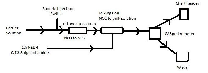
Flow Injection Nitrate Analysis When analysis Nitrate, a Nitrate Flow Injection Analysis was used with the equipment set up (as shown in the diagram) and the carrier solution - a saltwater matrix - was passed through the system and mixed with the sulphanilamide and NEDH. When mixed with the sample and the carrier solution created a pink solution. A premade standard of 10µM was tested first providing a peak that all the other samples could be compared with. The samples were passed through the system with the most saline samples tested first, reducing contamination because higher salinity water would have less nitrate due to increased uptake by organisms and fewer anthropogenic and weathering inputs. The higher the nitrate concentration, the bigger the peak. This was completed for all the samples and the two riverine end member samples from the River Allen and the River Kenwyn. The results showed with increased salinity there was a lower nitrate concentration.
|
![]()
![]()
![]()
![]()
|
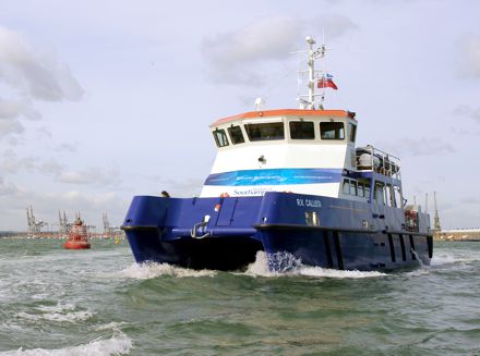
R.V. Callista R.V. Callista is a twin hulled research catamaran designed specifically for scientific research at the National Oceanography Centre. Equipped with both wet and dry labs on board and a large rear deck.
Specifications
Length: 19.75m |
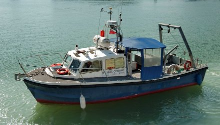
R.V. Conway
R.V. Conway is a purpose built Lochin39 vessel used primarily for teaching, research and surveying by the National Oceanography centre in conjunction with the University of Southampton.
Specifications
Length: 11.74m
|
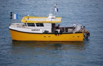
S.V. Xplorer The SV explorer; model Gemini-fastcat built in Colchester was used for the geophysics practical. This vessel was licensed by MCA (workboat Certificate category 2) and it allows the vessel to operate up to 60 miles from security.
Specifications Length: 11.88m |
|
 |
 |
 |
Estuary
![]()
![]()
![]()
|
The Fal Estuary acts as a transition zone between freshwater input and the sea. Biological, chemical and physical data were collected in order to understand how the estuary behaves. Our aim was to collect biological, chemical and physical data with temporal measurements on the King Harry Pontoon and spatial measurements aboard the R.V Bill Conway. Data collected along the Fal Estuary can be compared to the data collected offshore on R.V Callista. Constructing vertical profiles and sampling the water column at different positions along Fal estuary provides us with an overview of the estuary’s behaviour and its characteristics. The physical, chemical and biological data collected will allow us to establish this. The physical parameters measured include temperature, salinity and turbidity. These allow the physical structure and extent of estuarine mixing to be determined. In addition to these fluorescence measurements and nutrient variations can give an indication of the biological and chemical processes in the estuary. As an interface between freshwater and the coastal sea a transition in the data is expected to be shown. Data collected from this transect can be complimented by eulerian data collected from the King Harry Pontoon forming a more comprehensive temporal dataset for the estuary. Later this can be compared to the data collected offshore. A CTD system attached to a rosette frame was used to profile temperature and salinity. Also attached to the rosette were a transmissometer and a flurometer which measured turbidity and fluorescence. Three vertical profiles were constructed at three locations spread along the estuary. Using niskin bottles, water samples were collected at different depth intervals based on the maximum depth of the water column at each location. A hull mounted ADCP system recorded the current speed and direction along transects across the width of the estuary again in three different locations. A plankton net was used to collect a water sample of phytoplankton and zooplankton so the biology of the Fal could be analysed. A secchi disk was used to estimate the depth of the euphotic zone. Eulerian measurements were taken on the King Harry Pontoon using a Valeport Current Meter to measure current velocity, a LI-COR light probe to measure light intensity at varying depths and a YSI probe to measure temperature, salinity, chlorophyll concentration, depth, oxygen concentration and pH. The data from the pontoon was used to observe changes in the different properties over the tidal cycle. |
 |
|||||||||||||||||||||||||||
|
||||||||||||||||||||||||||||
Residence Time
|
|
|||||||||||
| Where: | |||||||||||
|
|||||||||||
|
The residence time is approximately 10 days. This is only an estimation because there are so many variables which are difficult to accurately record and measure, for example riverine flux was based on annual river gauge readings in the Fal, Kenwyn, Allen and Kennal whilst the total volume of the estuary was estimated from Admiralty charts 5602.5 and 5602.3. In the case of the Fal Estuary it is estimated that the impact of a pollutant depending on its toxicity, concentration and persistence could cause a significant short term impact on the estuary. |
![]()
![]()
![]()
|
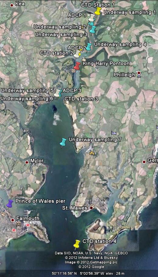
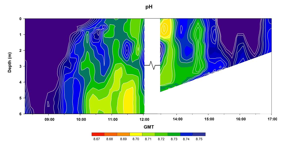
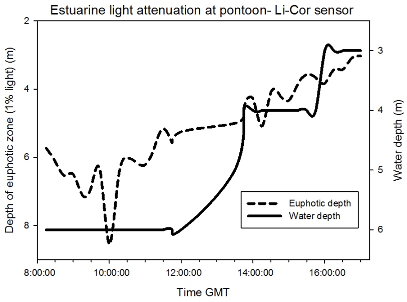
Eulerian measurements were made at 50.21618N, 5.02767W every 15 minutes from 08:15 GMT to 12:00 GMT. Measurements were continued from 12:30 GMT until 16:00 GMT by Group 6 to create a time series for the entire day. Measurements for current velocity and light intensity were made off the northern end of the pontoon and measurements made using the YSI probe were made off the East side. The YSI multiprobe measures temperature, salinity, chlorophyll, pH and dissolved oxygen. The King Harry Ferry passes by every 15 minutes creating a large wake; this could lead to less stratification than expected in the water column than expected. The data from the pontoon was used to observe the changes in the water properties over the tidal cycle with time. High tide was at 09:33GMT and low tide was at 15:05GMT consequently for the majority of the sampling time water flow was to the south. Method The YSI multiprobe was deployed from the pontoon every 15 minutes, suspended at first in surface waters and then lowered through the water column at 1 metre depth intervals, reaching 6m depth. The data and depth from the YSI probe was monitored using the hand-held data receiver, to which salinity, temperature, chlorophyll, pH and dissolved oxygen measurements were automatically relayed to the data logger. The accuracy of the YSI probe is affected by the slight time-lag between the depth sensor and the data relay system, as the deployment line itself is not marked with metre intervals. The Valeport current metre was also deployed at 15 minute intervals from the pontoon, the metre orientated itself according to the direction of flow and the flow powered the rotating turbine at the rear of the meter. Unlike the YSI, the line of the current metre was marked with 1m intervals. When measuring light intensity one sensor remained at surface level, measuring the light intensity above the water surface, while the second light sensor was lowered through the water column at 1m intervals, down to 6m. This combination of light sensors ensured that the light intensity measurements at depth could be compared to that of the surface and so variation in light intensity over the day could be monitored. Tides |
||||||||||||
|
||||||||||||
|
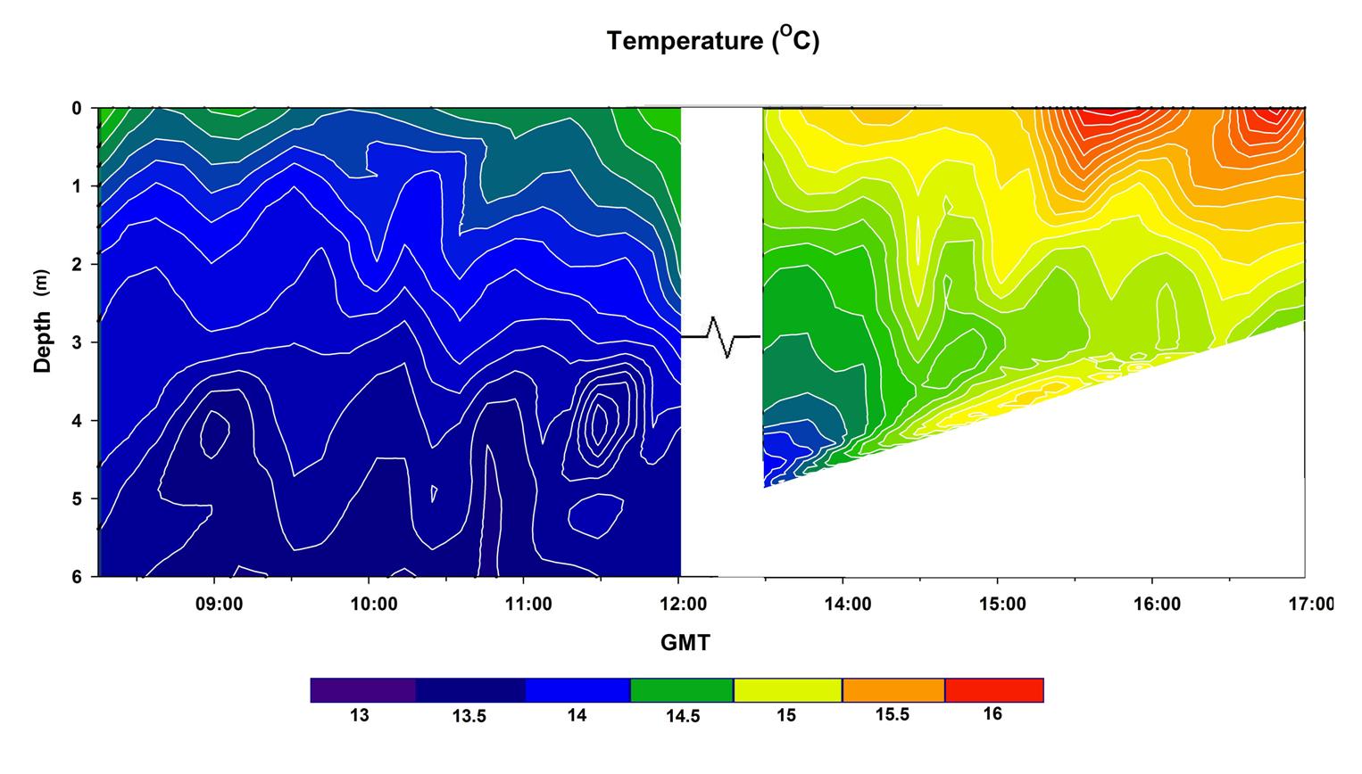
Temperature First sampling session between early hours of 08:15 and 12:00GMT, local weather around the pontoon was misty. Solar warming effect was low between these hours but evident as there was a warmer layer on the top between 0 -1m; evidence of a partially mixed estuary. The temperature declines with depth. The second sampling session ran between 13:00-17:00GMT, when the temperature of the estuary increased becoming progressively more stratified until 15:00GMT. This is due to an influx of warmer fresh water where insolation had had a greater effect upon a smaller body of water. A temperature gradient may be observed with time; at 16:00GMT a relatively warm body of water was evident between 0-2m. These are typical characteristics of a ria estuary. |
 |
Salinity
|
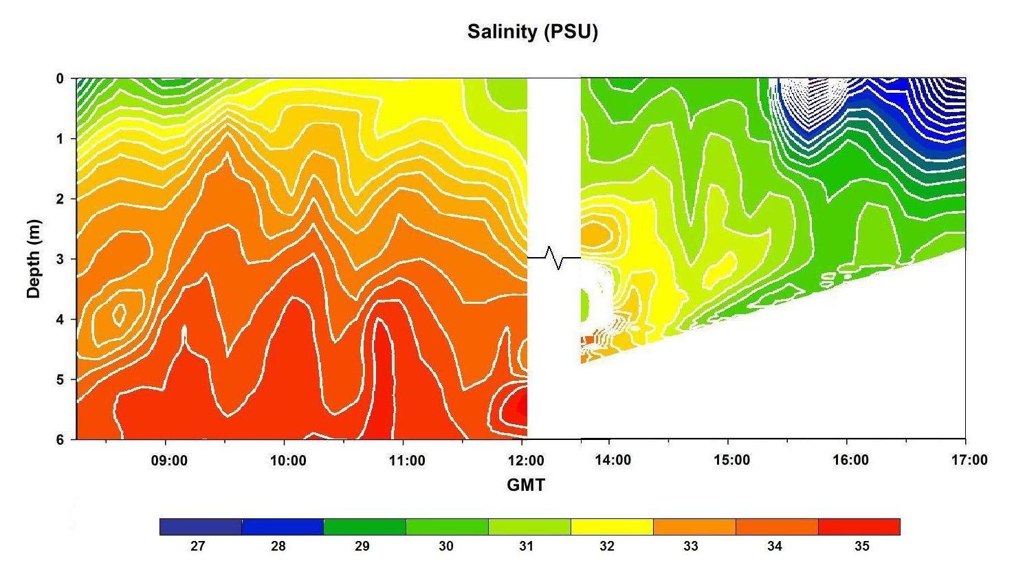
Due to the dominant influx of seawater prior to high water at 09:22GMT, samples collected between 08:15-12:00GMT show partially mixed water column where salinity increases with depth. A lower reading of salinity in surface water was detected due to seawater being higher in density than freshwater. The second sampling began during ebb tide, allowing the influx of freshwater to dominate. This created a partially mixed estuary between 14:30-15:30GMT before a large input of freshwater resulted in stratification to create a region of freshwater from 15:15GMT onwards that increases as time progresses. |
 |
Chlorophyll
|
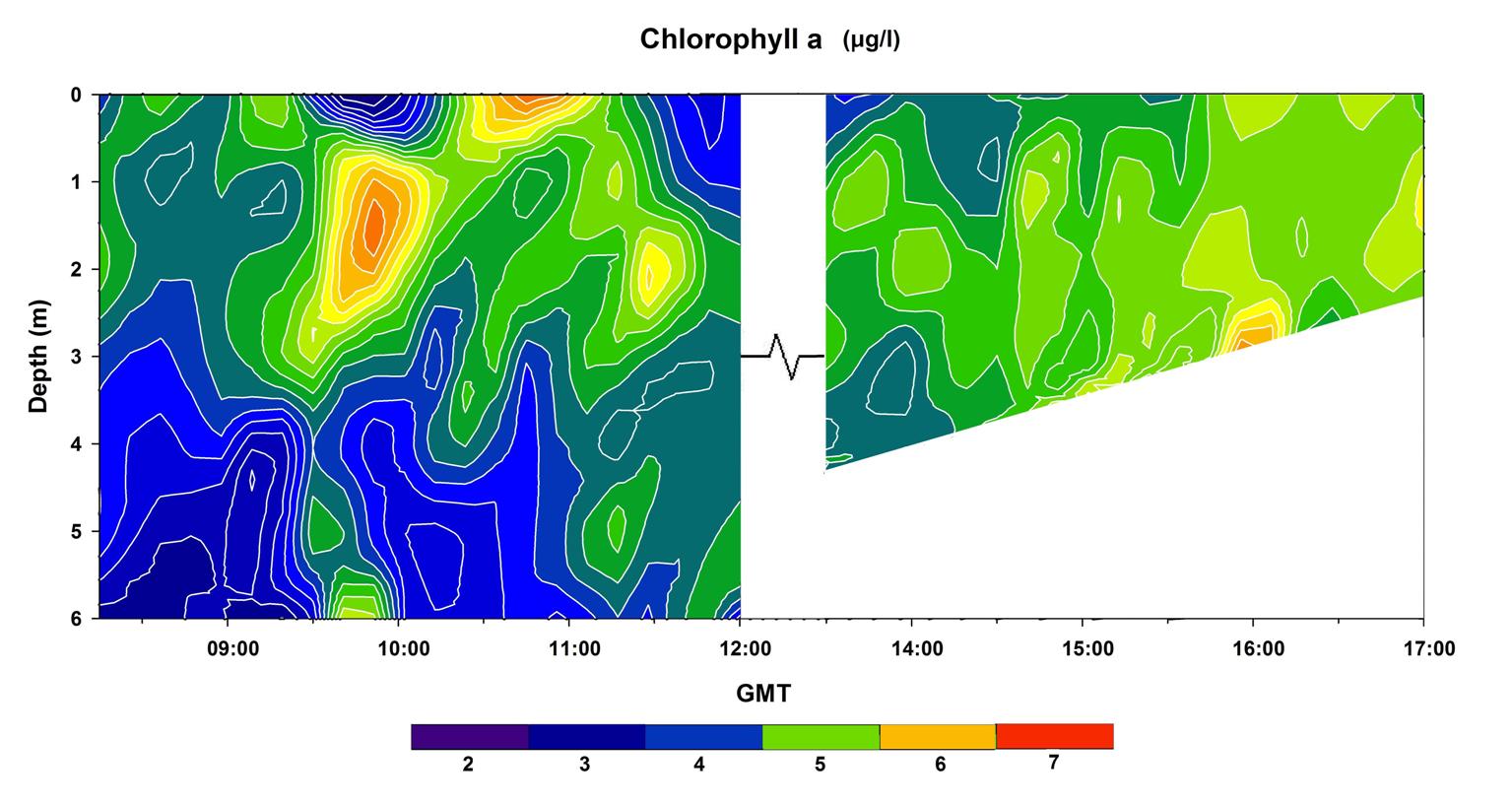
Chlorophyll levels increased slightly throughout the day. Levels appeared to be higher above 3-4m, perhaps due to high turbidity shading. There were patches of increased chlorophyll, such as around 2m just prior to 10am. This could be caused by localised blooms, particularly of dinoflagellates, which have sufficient motility to maintain proximity to a preferable water parcel. |
 |
|
pH pH exhibited minimal change throughout the tidal cycle. This is to be expected as seawater tends to have a fairly stable alkalinity, predominantly due to the bicarbonate buffering. However, small changes are still noteworthy because pH is a logarithmic scale and thus incremental changes are relevant. River water has a lower pH, so in the pH contour plot, maximum values were observed at flood tide periods, with seawater pushing through to dominate the pH. During the ebb tides, pH was at its minimum. |
 |
|
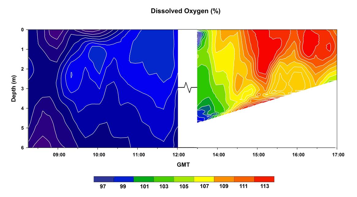
Dissolved Oxygen
Dissolved oxygen increased throughout the day. The principle factor affecting oxygen levels is planktonic life, due to respiration and photosynthesis. Phytoplankton, whose photosynthesis produces oxygen, can be estimated by chlorophyll- which increased throughout the day. Light levels also increased throughout the day, peaking in the early afternoon. This whould have caused higher levels of photosynthesis, and explains greater of oxygen levels. |
 |
|
|
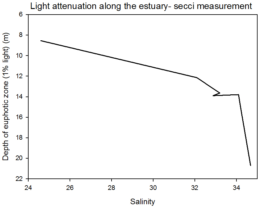
Light
The surface light levels throughout the day (26/06/12) were very varied, due to the changing cloud cover. Light attenuation was recorded at 15 minute intervals at individual depths to calculate the depth of euphotic zone. The euphotic zone decreased in depth as the tide receded. Due to the turbidity sensor on the YSI probe not being functional, it is hard to be certain of the cause of this. Boat readings show that more saline water meant less attenuation. It is likely that the turbid river water that was more dominant at an ebb tide lowered light penetration.
|
Estuarine Transects aboard R.V. Conway
![]()
![]()
![]()
![]()
|
Aboard R.V. Conway data and samples were collected at several stations by way CTD casts with niskin bottle sample capture, Plankton trawls, ADCP transects and collection of surface samples underway with changes in salinity. Data collection began at the top of the estuary near Malpas and then continued moving down the estuary, working against the flooding tide, to ensure different water bodies were sampled at each station. Group 3 continued the data sampling of the estuary after the high tide, moving from Black rock at the estuary mouth upstream against the then ebbing tide. Methods Underway The horizontal and vertical water samples were collected using a impeller water pump and a CTD rosette. The silicon, nitrate, phosphate and chlorophyll concentrations of each water sample were analysed; additionally the concentration of dissolved oxygen in CTD samples were fixed for further analysis by the Winkler method. The over side pump was used specifically to collect water samples every one unit of salinity. Nutrient Samples Both the horizontal and vertical transect water samples were prepared for nutrient and chlorophyll analysis on-board the R.V. Conway. Volumes of 50ml were removed from the sample and filtered using a 25mm glass microfiber filter into plastic and glass bottles for silicon, nitrate and phosphate respectively, for future lab analysis. Resulting in approximately 20ml of water for silicon and 25ml in each nitrate and phosphate bottles, the remaining volume was used for instrument rinsing. The 25mm filter from each syringe was removed and stored in 90% acetone, which breaks down the cell walls of phytoplankton, resulting in the release of chlorophyll. This process was then repeated in order to create a replicate chlorophyll measurement, where the filtrate was dispensed into the nitrate and phosphate bottle for further laboratory analysis. The concentration of dissolved oxygen was fixed using 1ml of each of manganous chloride and alkaline iodide solution. On addition of the alkaline iodide, a dense yellow/orange precipitate formed. The stopper was inserted sharply to minimise air interaction and the bottle was inverted continuously for 30 seconds to ensure complete mixing. The bottles were then submerged in water to prevent oxygen interference during storage. The silicon samples were collected from the R.V. Conway using both the over the side water pump system and a CTD rosette. The samples were stored in plastic bottle under cool conditions. Plankton Samples Lugol’s iodine preservative was added to a 100ml volume of surface water sample for further microscope analysis. The 100ml water sample was dispensed using a measuring cylinder to prevent cell disruption. A further 100ml of water was removed from the sample and stored in a separate container, to which, the preservative formalin solution was added for future lab observation. Two plankton net trawls were undertaken in order to collect zooplankton species at different points along the estuary at differing tidal states. The first trawl was done as far up the River Truro as R.V. Bill Conway could reach, near Malpas, on the flood tide. The second trawl was completed at the confluence of the River Truro and Carrick Roads; off Turnaware Point, close to high tide. The net was towed at slow speed (0.7 m/s) for five minutes in both instances. It was held just below the surface. The current flow meter that measured flow through the net had values noted prior to and subsequent to the trawl (1 revolution equated 0.3m). In order to calculate the volume of water that was filtered during the trawl, revolutions multiplied by 0.3, multiplied by the area of the net entrance (0.25m2π). The mesh size was 210µm, so zooplankton of a size larger than this should have been collected in the end bottle. Anything attached to the net was rinsed off into the container, transferred to a bottle, and fixed with 10% Formalin solution. |
||||||||||
|
||||||||||
|
CTD Data (Click graphs to enlarge) |
||||||
 |
 |
 |
 |
|||
|
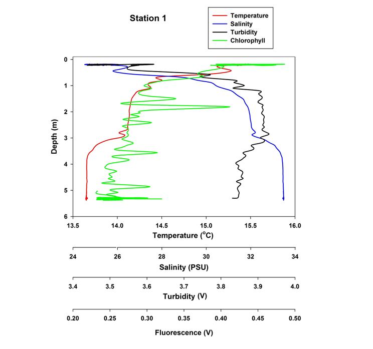
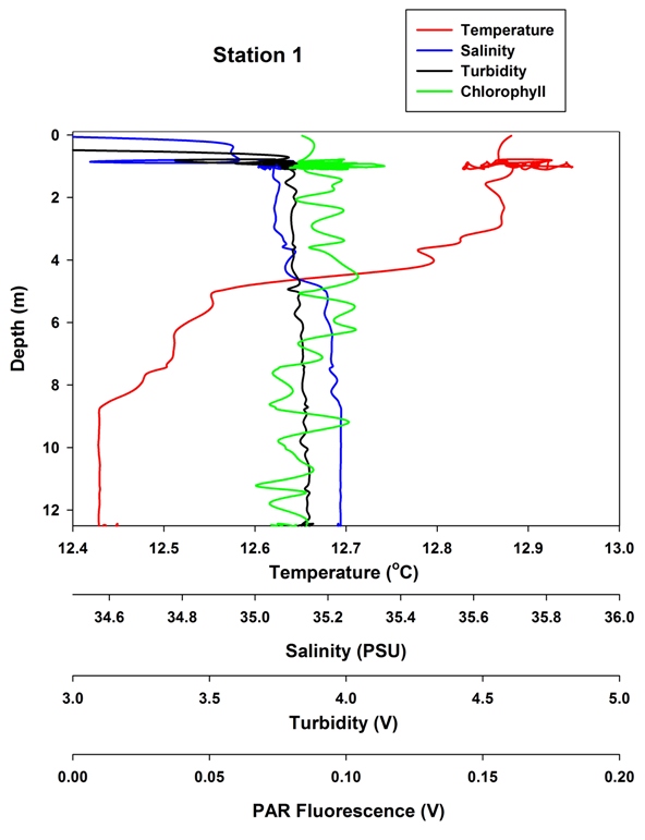
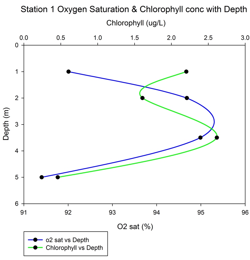
Station 1 Salinity values for the estuary are at their lowest here, particularly at the surface (~24 PSU) which is to be expected because of the increased proximity to fresh water inputs. As depth increases the saline coastal water starts to have more of an influence and the overall salinity increases. Temperature decreases with depth through a combination of less light energy penetrating into the water column and by mixing processes dissipating heat energy as warmer surface water is mixed with cooler water below. Both temperature and salinity profiles show stratification in the water column at approximately 3m after this both profiles are uniformed with depth. The chlorophyll profile exhibits an overall negative trend. Chlorophyll concentration decreases as phytoplankton populations decline with depth. There is a turbidity maximum at the surface, possibly caused by higher phytoplankton concentrations and air-sea interactions (dust particles etc). Turbidity then shows a decrease with depth, arguably because of less biology being present in the water column. |
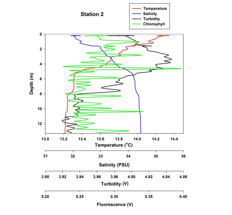
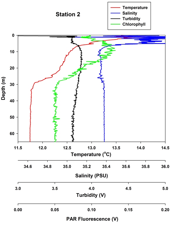
Station 2 Station 2 shows salinity and thermal stratification up to around 5m, whereupon both variables become constant in a well-mixed parcel of marine water. Up until this depth temperature decreased and salinity increased. Salinity reaches a maximum of approximately 34.5 PSU at this station. Unlike station 1, the water becomes more turbid with depth which is likely to be due to tidal flow over the water-sediment interface re-suspending particles through shear stress, as this sample was taken at 09:28GMT on the flood before HW at 11:26GMT. Chlorophyll was noisy but constant; never fluctuating by more than 0.1V if noise is ignored.
|
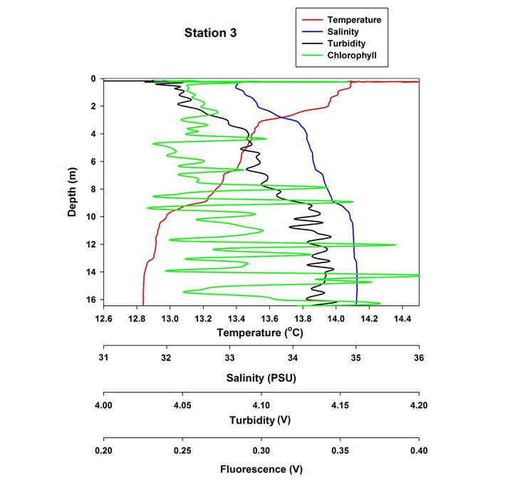
Station 3 There was a gradual temperature decline from ~14.2°C at the surface to 12.8°C at 10m depth and salinity increases from 33 to 35. Because station 3 was further out into the mouth of the estuary it explains why freshwater dominance is confined to approximately the top 3 meters and why salinity/temperature change more quickly with depth although no real thermocline is yet apparent. Salinity in the surface layer could have been influenced by the recent high precipitation rates, consequently it could be lower than expected for this time of year. This sample was taken during slack water and the transmissometer data reflects this as turbidity is low near the sediment-water interface. This could also illustrate the stability of the stations permanent marine bottom member whereas tidal mixing is reduced further out into the estuary. Chlorophyll is again noisy, but more or less constant.
|
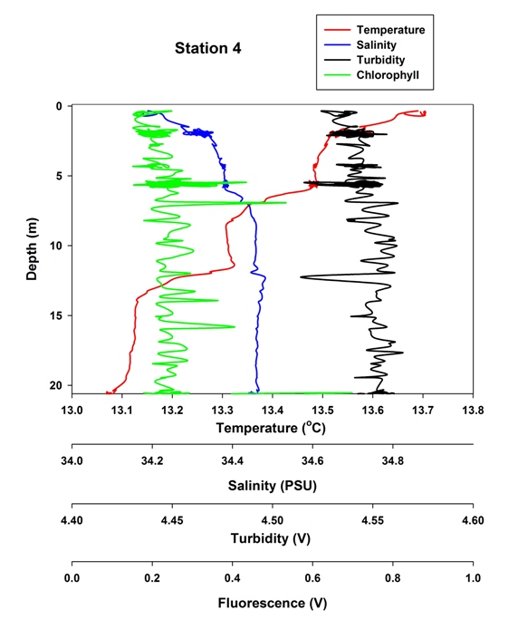
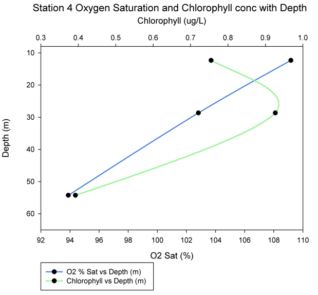
Station 4 Station 4 was in the mouth of the estuary, near Black Rock. Chlorophyll and turbidity are constant through the water column, which is completely saltwater dominated (~34 PSU). A water sample from this station could be considered as an end-member. The water column remains thermally stratified as there is still no evidence of a true thermocline and so whilst this station may be regarded as a marine endmember it is not far enough out to sea for thermal stratification to overcome the effects of tidal mixing.
|
Dissolved Oxygen Analysis
|
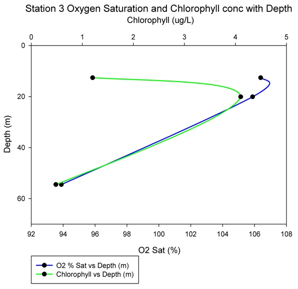
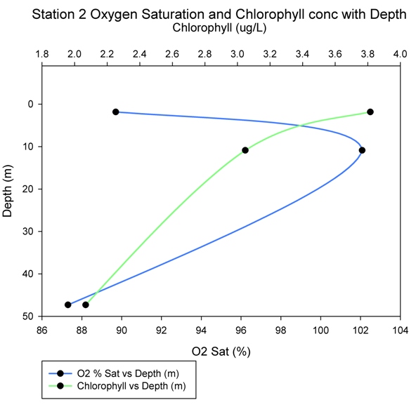
The saturation level of oxygen in the water column is dependent on multiple variables. Production of oxygen is mostly determined by phytoplankton concentration; larger phytoplankton blooms are commonly associated with higher oxygen levels. Phytoplankton is represented by a chlorophyll proxy. Consumption of oxygen is ordinarily caused by respiring zooplankton and substances with a high oxygen demand. Overall oxygen saturation levels increase along the estuary towards the mouth. Station 1 in the upper estuary showed low oxygen levels in the upper part of the water column (~1m) this is could be because of oxygen demanding substances being present in the surface layer. Oxygen increases with depth and correlates well with chlorophyll, peaking at about 3m, before both parameters decrease. In the mid estuary at station 3 the vertical profile again shows a close correlation between oxygen and chlorophyll concentrations. After peaking at 114%, oxygen saturation drops rapidly at ~12m. This coincides with the 1% light level (~14m) where chlorophyll declines rapidly. Station 4 at the estuary mouth there is relatively lower chlorophyll levels possibly due to lower nutrients nearer to saline end-member and higher zooplankton predation. However oxygen saturation in the water column here is at its highest. As well as phytoplankton oxygen production these levels could also be influenced firstly by light levels increasing throughout the day, peaking early afternoon. This can cause higher levels of photosynthesis, and therefore greater production of oxygen. Secondly lower nutrient concentrations and less oxygen demanding substances being present would result in less oxygen consumption and a higher percentage saturation.
|
Click to enlarge
Station1
Station3
Station4 (No sample at station 2) |
N:P Ratio
![]()
![]()
![]()
![]()
|
|
Nitrate
|
|
|
|
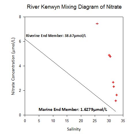
Estuarine mixing diagrams for Nitrate in the Fal estuary indicate non conservative behaviour. All the Nitrate concentrations measured on the Fal are above the TDL indicating that Nitrate is being added to the water column. The highest Nitrate concentration 7.44 µmol/L was found at a salinity of 25.8 and the lowest concentration of 1.16 µmol/L was found at a salinity of 32.4. The addition of Nitrate into the Fal could be due to agricultural runoff and leads to hypernutrification of the Fal. This has led to the Fal being designated a ‘sensitive area’ under the Nitrates directive 91/676/EC (accessed: www.mba.ac.uk/nmbl/publications/charpub/pdf/Fal_Helford.pdf , 5th July 2012). |
Phosphate
|
|
|
|
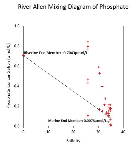
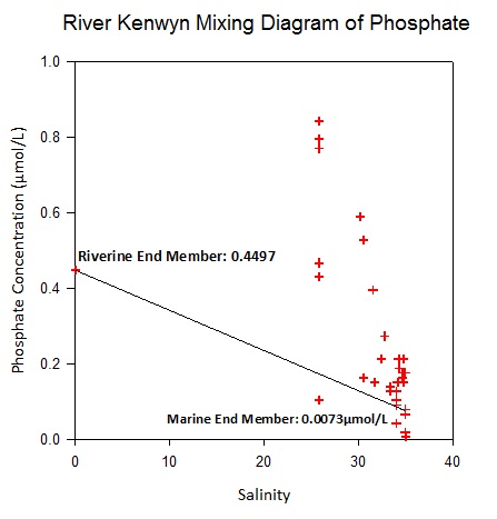
Phosphate concentrations in the Fal estuary are far removed from the TDL and exhibit non conservative behaviour. The Highest phosphate concentration is 0.84 µmol/L at a salinity of 25.8. The lowest concentration of phosphate is 0.0073 µmol/L at 35.0 salinity. The increase in phosphate above the TDL indicates that phosphate is being added to the water column, anthropogenic factors such as agricultural run off or the input of sewage into the Fal estuary. The West Country Mussel Farm near the King Harry Pontoon could also affect phosphate concentrations in the water column. The aforementioned mussel farm was surveyed by Envirogene, this survey established that the water of the Fal estuary was contaminated by human and bovine faeces. It was identified that at the King Harry Ferry there was a significant input of faecal matter into the Fal. (accessed: www.envirogene.co.uk/downloads/casestudies/envirogene_case_fal.pdf , 5th July 2012). |
Silicon
|
|
|
|
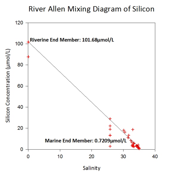
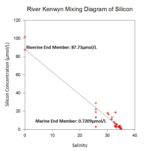
Silicon concentrations increased with decreased salinity reflecting an inverse correlation with the greatest concentration found at 29.07 µmol/L at a salinity of 25.8. The lowest silicon concentration was 0.72 µmol/L at a salinity of 35 which was at the highest salinity. Overall the behaviour of silicon in the Fal Estuary was conservative, although there was some slight deviation from the Theoretical Dilution Line (TDL), for example at a silicon concentration of 2.37 µmol/L at 25.76psu, this is likely to have been an anomaly. The conservative trend showed that silicon concentration was determined by the mixing of riverine and marine end members rather than estuarine chemical processes. |
Plankton Trawls
![]()
![]()
![]()
![]()
|
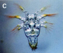
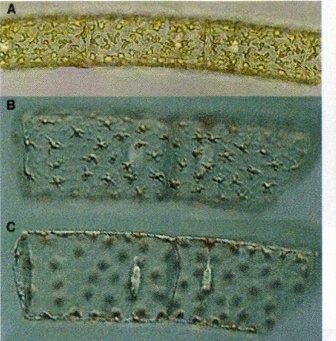
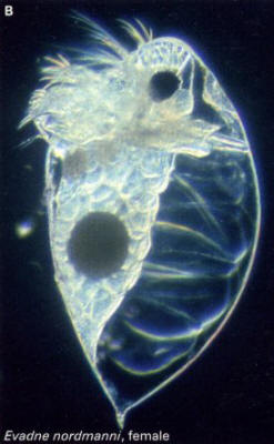
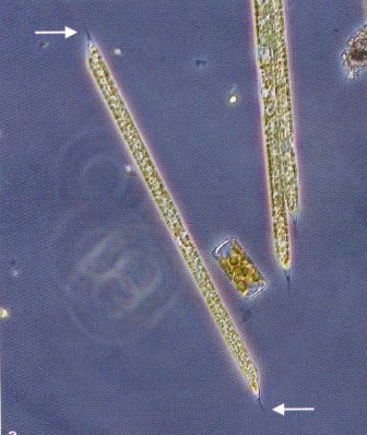
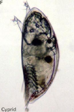
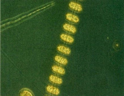
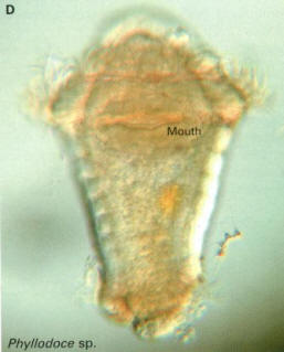
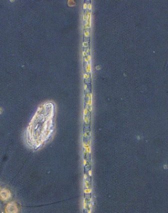
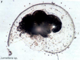
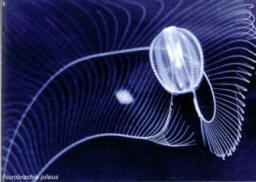
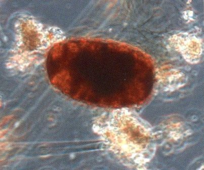
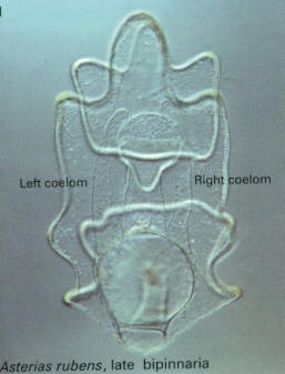
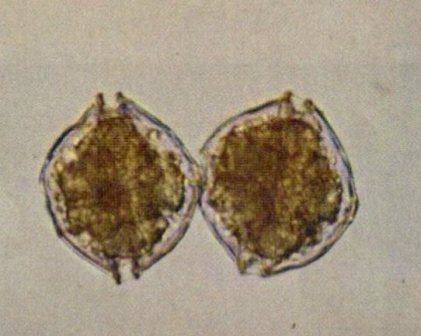
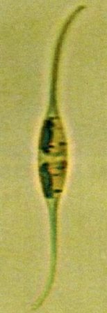
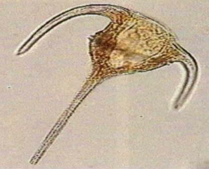
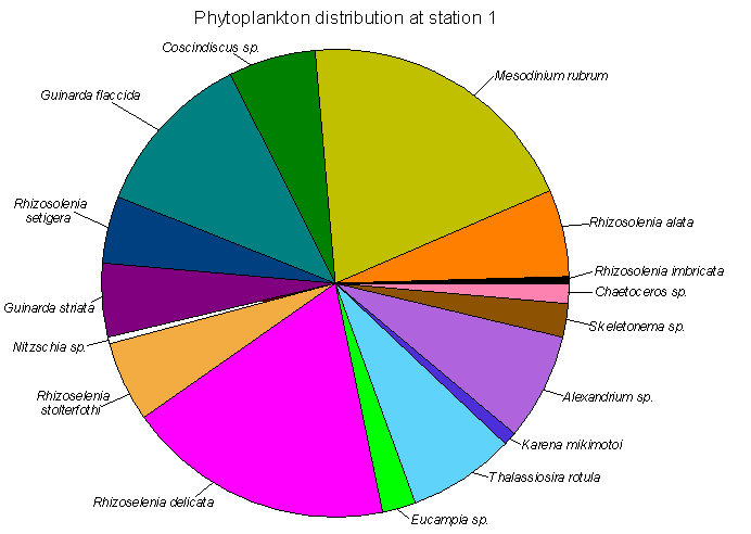
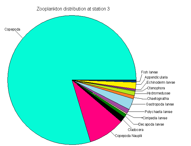
Phytoplankton counts The phytoplankton preserved in Lugol’s iodine solution from station 1 was placed in a glass sedimentation chamber and left overnight. Only the bottom 10ml of the 100ml water in the chamber is kept and the other 90ml discarded. A Sedgewick-Rafter Counting Chamber was used to count the phytoplankton in 1ml of water i.e. there were 10 replicates. 5 columns of 20 cells were counted and the phytoplankton identified in each chamber. The percentage of phytoplankton (see graph below) showed that the population consisted of a variety of species with the two most populous groups being Mesodinium rubrum and Rhizoselenia delicata comprising 19.9% and 18.5% of species found respectively. Zooplankton counts Using stereomicroscopes, 10ml of plankton preserved in formalin was counted and identified in Bogorov-trays. There were 3 replicates on the two plankton trawls and so the zooplankton was identified in 30ml of each sample. The distance sampled by the plankton trawl was calculated using the flow volume, diameter of net and current. Therefore, the total number of zooplankton per m3 in the water sampled was calculated by diving the total by 41 for bottle x and 37 for bottle y. The percentage that each zooplankton group attributed to the total was calculated. In bottle y, there was a total of 217,887.00 zooplankton per m3 whereas there were 85,000 zooplankton more per m3. The zooplankton composition was similar at both sites with three groups (see graph below) . At Station 1, bottle z the three dominant groups were copepoda (76.5%), copepod nauplii (13.4%) and cladocera (4.85%) whereas at bottle x at station 5 the three dominant groups were copepoda (79.7%), copepod nauplii (9.19%) and gastropod larvae (2.79%). The large amount of the copepods in both samples reflects the high abundance and dominance of the taxon throughout the ocean. The cladocera was dominant in fresher waters whereas the gastropod larvae became more populous at station 5 in more saline waters and near the shellfish farm. |
|
|
|
Plankton Guides
|
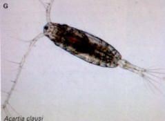
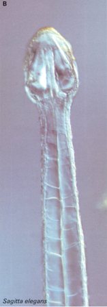
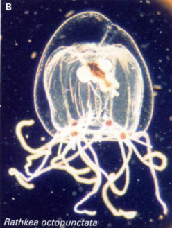
Zooplankton (Larink & Westherde, 2006)
|
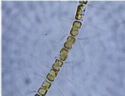
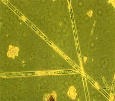
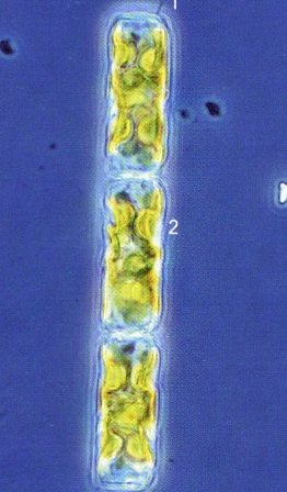
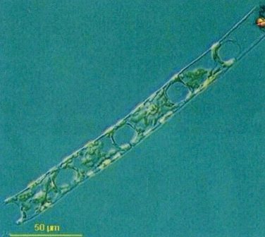
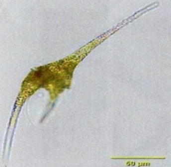
Phytoplankton (Kraberg et al., 2010)
|
|||||||
| Copepoda | A large taxon comprising many species with high
abundance globally. Range in length from 0.5 to 5mm.
Identifiable by a large cephalothorax, shorter and narrower
abdomen and the presence of two pairs of antennae. |
 |
Chaetoceros | Cells either solitary or connected into short chains. Long stiff setae
originate from the cell margins. Chloroplasts numerous. 8-50µm
in diameter. Coastal distribution. |
 |
|||
| Copepoda Nauplii | The larval stage of copepod development. Often the
body is more stunted with the legs often clearly visible. There
are often multiple stages of nauplii growth.
|
 |
Guinardia flaccida | Cells cylindrical and colonial, forming a straight chain. Distinct
bands visible between cells as well as star shaped chloroplasts
in cells. 45-160µm in length. Coastal distribution. |
 |
|||
| Cladocera | Cladocera or water fleas are crustacean that have
relatively short head and thorax sections with an almost or
completely unsegmented abdomen. A key identifying feature is the
single compound eye in the middle of the head. 0.2mm up to 1.1mm
in length. |
 |
Rhizosolenia imbricata |
Cells long and cylindrical with an extremely long pervalvar axis with a pointed wedge shape at the ends of the cell. Up to 650µm in length. Coastal distribution.
|
 |
|||
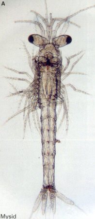
| Mysidacea |
Mysidacea are shrimp like and are between 2 and 30mm long. The Mysidacea can be easily identified by the visible statocysts in their uropodal endopodites. Females can be identified by the presence of brood pouches on the ventral side of the thorax.
|
 |
Rhizosolenia setigra |
Cells long and cylindrical with a slightly broadened base and tapering towards the ends of the cell. Up to 600µm long. Coastal distribution.
|
 |
|||
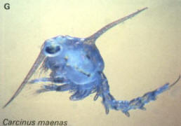
| Decapoda Larvae | Decapoda larvae are highly diverse in their shape
and the way they develop. Zoёas is a generic name for these
larvae and they can often be identified by a carapace that
covers the head and anterior thorax, often this carapace can
have prominent spines. |
 |
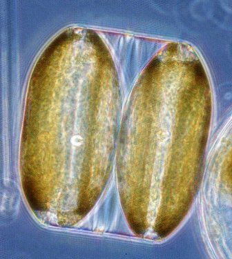
Coscinodiscus | Cells boxed shaped in girdle view but circular in valve view. Each
cell contains multiple chloroplasts either in a section or two
separate compartments. 80-400µm in diameter. Coastal
distribution. |
 |
|||
| Cirripedia Larvae | Nauplii of cirripedia are easy to identify. These
are the juvenile stages of barnacles found free swimming in the
water column. They can be identified by a carapace with two
fronto-lateral horns. Meanwhile the first antennae are equipped
with long distal cuticular spines that can act as effective
paddles. |
 |
Thalliosiosira | Multiple pill shaped cells aligned in a chain with each cell connected
to the chain by a thread. 12-100µm. Coastal distribution.
|
 |
|||
| Polychaeta Larvae |
The typical Polycheate larvae are the trochophora. Often is made up of a spherical prototrochophore covered in short cilia, a band of cilia called the prototroch encircles the body anterior of the mouth. These trochophora develop from the posterior. Sizes range from 70µm to 2mm. |
 |
Leptocylindrus danicus | Cells long and cylindrical with a circular cross section connected
into long straight chains of cells. 20-50µm in length. Coastal
distribution.
|
 |
|||
| Gastrapoda Larvae |
Gastropod larvae develop from trochophores, similar to polycheata larvae. However gastropod trochophora are often not spherical and possess a prototroch anterior to the mouth with an apical tuft of cilia. The majority of gastropods have a shell, protoconch, which extends over their veliger. Sizes range from 280µm up to 1mm |
 |
Rhizosolenia alata | Cells long and cylindrical with curved valves which taper into a blunt
ended proboscis. Cells are often solitary but can be joined into
short chains. Contain numerous small chloroplasts. Up to 700µm
in length. Coastal distribution. |
 |
|||
| Chaetognatha Larvae |
Chaetognatha or arrow worms are transparent and easily identifiable by their elongated and unsegmented body shape.
|
 |
Guinardia delicatula | Cylindrical and slightly rounded valve faces with cells formed into a
close set chain containing irregular lobed chloroplasts each of
which has a pyrenoid. 20-70µm in length. Coastal distribution. |
 |
|||
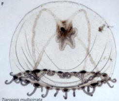
| Hydromedusae Larvae |
Hydromedusae larvae are gelatinous medusa containing identifiable gonads surrounding a central mouth. The outside edge of the medusa is ringed by tentacles containing nematocytes. The medusa is between 300µm and 2mm, not including tentacle length. |
 |
Eucampia | Cells have a trapezoid outline with very concave valve faces. The
cells join together in a helical chain containing multiple small
chloroplasts. Each cell is 10-100µm in size. Coastal
distribution. |
 |
|||
| Siphonophorae |
Unlike medusa the Siphonophorae are colonies and not individuals. The anterior end of the axial polyp forms a gas-filled float in some Siphonophorae. They are all planktonic and can grow up to several metres in length. |
 |
Ceratium furca | Dorso-ventrally flattened cells with a tapered epitheca ending in an
anterior horn and a tapered hypotheca that ends in a long left
and short right antapical horn. 150-230µm in length. Coastal
distribution. |
 |
|||
| Ctenophora |
Ctenophora are typically 1mm up to 10cm long and they have biradial symmetry. They have cilia for movement and their tentacles are extended from pouches. |
 |
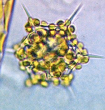
Polukrikos | Large pseudocolonial species that consists of zooids in set group
numbers formed in a roughly cylindrical shape. 60-100µm in
length. Coastal distribution. |
 |
|||
| Echinoderm Larvae |
The entire surface of the early echinoderm larva is covered in cilia and they can be identified by the envaginating pouch forming the blastocoel at the blind end of the archeteron. Eventually the cilia become restricted to a continuous band and the body can form extensions like arms and lobes. 100µm to 2mm in size. |
 |
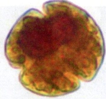
Alexandrium |
Spherical cells that have a slight protruding apical pore complex
clearly visible on the light microscope. The cells also contain several
red-brown chloroplasts. 35-69µm in diameter. Coastal distribution. |
 |
|||
| Appendicularia |
The Appendicularia are a subtaxa of the Tunicata and are fairly transparent. Unlike the Chaetognatha they have a ‘house’ of mucous which is often not observable in collected samples. They have large ‘tails’ with a shape resembling tadpoles and range between 0.6 and 4.5mm. |
 |
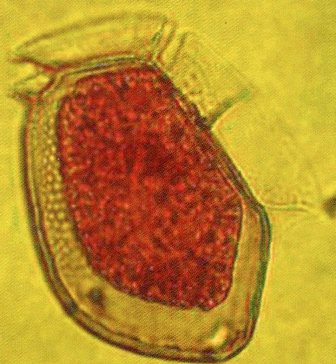
Dinophysis |
Cells laterally flattened with a broad left sulcal list which extends down the cell. The thecal plates are also strongly areolated. 40-100µm in length. Coastal distribution.
|
 |
|||
| Marine teleosts produce eggs during reproduction. These eggs are about 1mm in diameter and consist of a chorion surrounding the main egg. Often they can also have a micropyle. The hatched larvae often still have an attached yolk-sac . |
 |
Karinia mikimotoi | Cells oval shaped and dorsoventrally compressed. A clear straight
apical groove is present and the cells Sulucus is also straight
and passes up into the epicone. Cells are 18-37µm in length.
Coastal distribution. |
 |
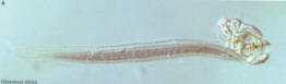
||||
| Distephanus | Cells are formed around a silica skeleton uniflagellate consisting of
two differently sized hexagonal rings with 6 long spines on the
outer ring and 6 shorter on the inner ring. The cells are
19-35µm in diameter, not including spine length. Coastal
distribution. |
 |
||
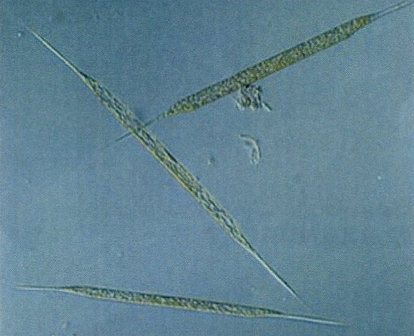
| Nitzschia | Spindle shaped cells with pointed ends and highly silicified structure
containing visible poroids. Cells colonize as stepped chains and
contain two plates like chloroplasts. 75-140µm in length.
Coastal distribution. |
 |
||
| Ceratium tripos | Assymetrical cells with a straight apical horn with closed distal ends
and two antapical horns which bend around the cell until they
are parallel with the apical horn. Up to 300µm in length.
Coastal distribution. |
 |
||
| Ceratium fusus | Needle shaped cells with an elongated curved outline. The wider
cingulium contains the chloroplasts. Epitheca tapers into a long
anterior horn but hypotheca tapers into a very long left horn
and stub like right horn. Cell is 150-230µm in length. Coastal
distribution. |
 |
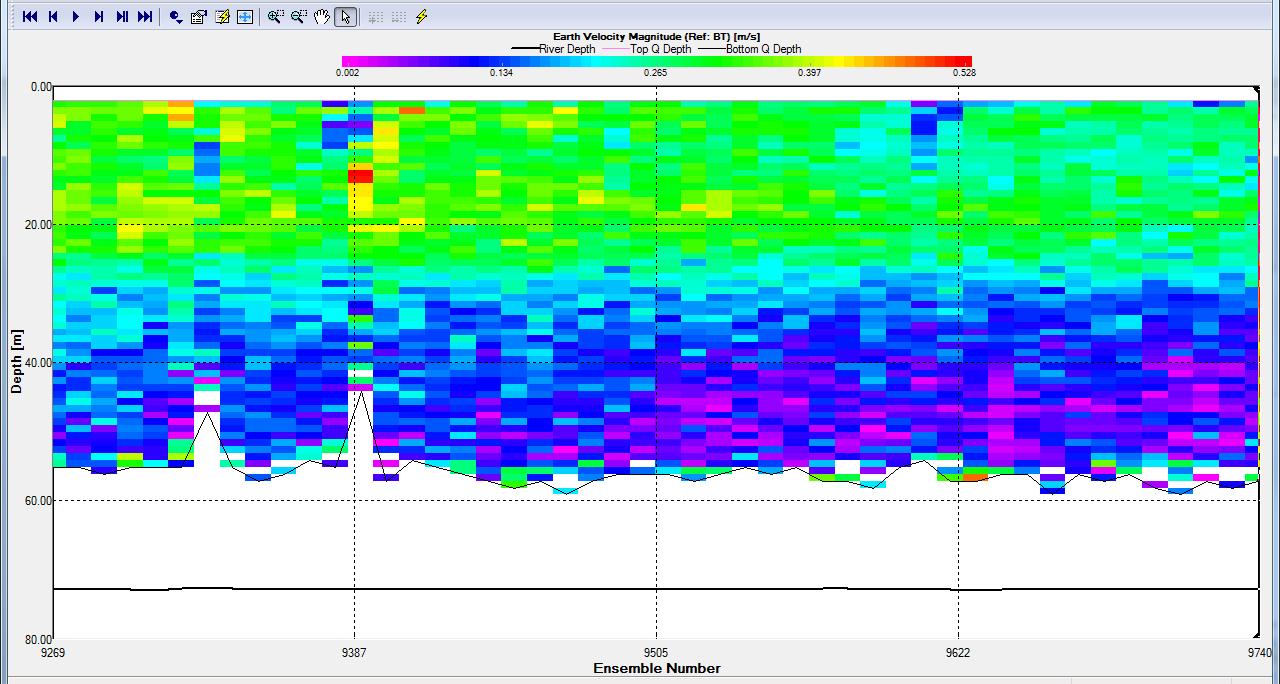
ADCP
![]()
![]()
![]()
![]()
|
The Richardson number is a dimensionless value that indicates the stability of the water column, calculated from the ratio between the stabilising effect of the density gradient and destabilising effect of the velocity shear, and the is used to determine the amount of mixing within the water column. Richardson number Calculation:
Where g=gravity (ms2) h=depth u=velocity (ms2)
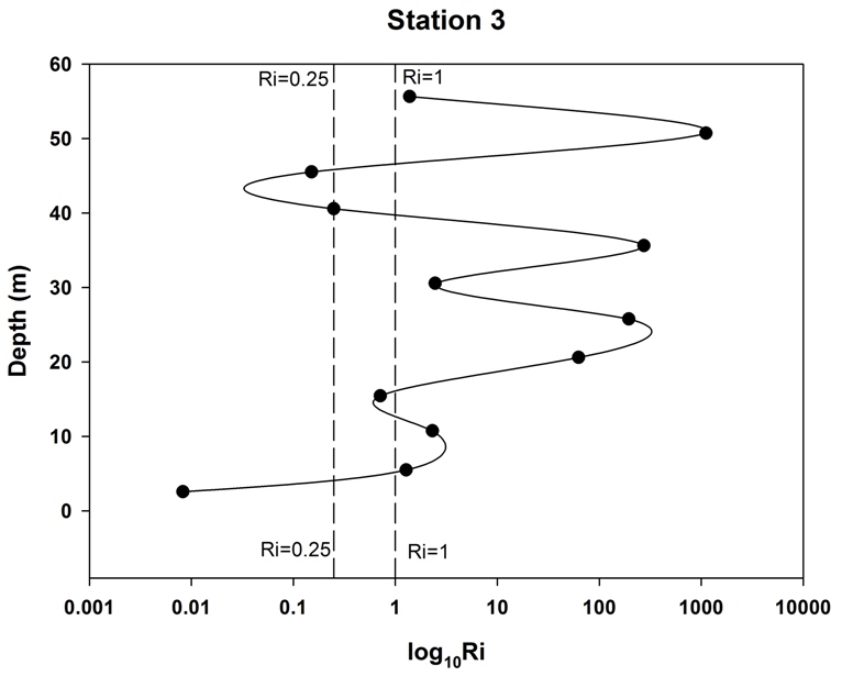
When the Richardson number is <0.25 the water column can be described as instable, where shear occurs between the water layers as a result of a difference in the average velocity, resulting in a break down in stability and overall turbulent conditions. When the Richardson number is much greater than 0.25 conditions within the water column can be described as stable and when between 0.25 and 1 the water column is likely to be stable yet the cut of value can not be well defined. |
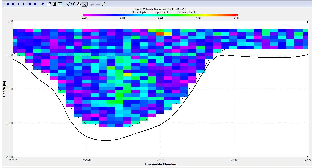
Station1
|
Location: Lat 50o14.400N Long 005o00.877W
Therefore the Ri number at Station 1 on the estuary indicates turbulent mixing and instability within the water column.
click to enlarge click to enlarge
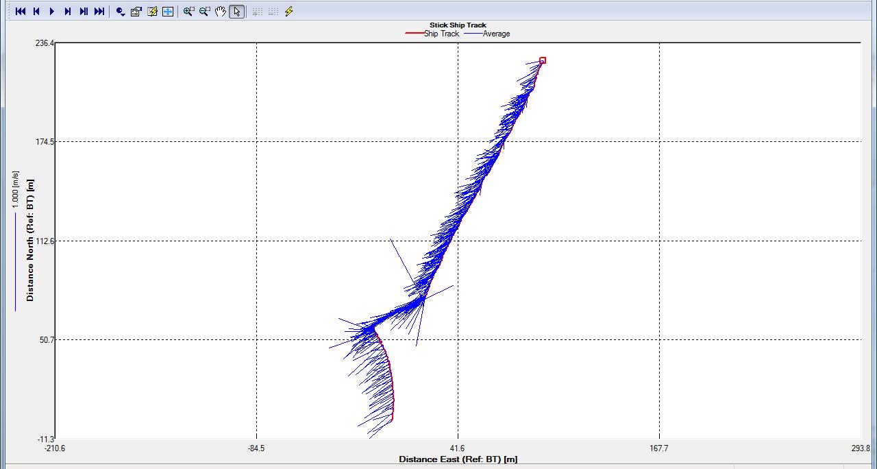
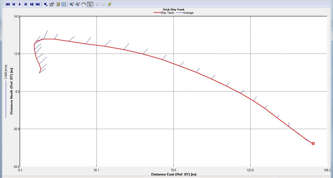
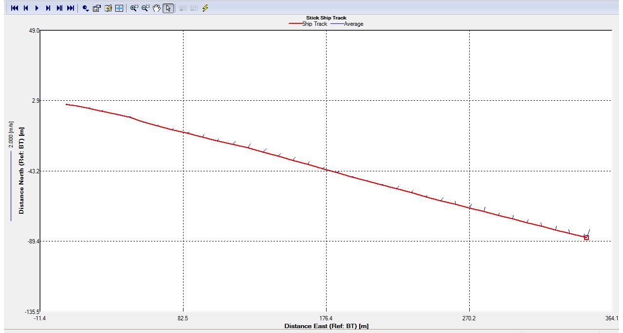
The change in direction of the ship track indicates change in direction of the vessel as we travelled to the source river and sampled coming back up the estuary. The average of the ship track does not vary greatly in direction over the transect and therefore, does not indicate the presence of shear within the water column. The lack of shear is a direct result of sampling a shallow area of water where overall mixing of the water column has occurred, which is supported by the Richardson number of 0.
click to enlarge
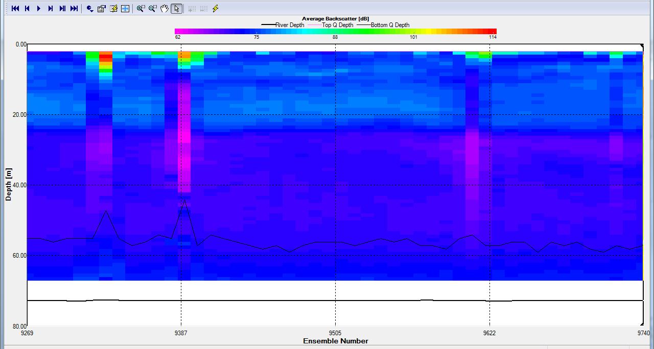
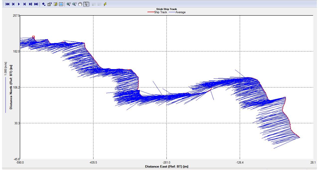
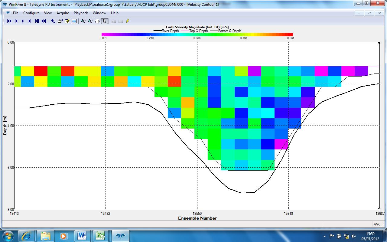
Station3 Location: Lat 50o12.240N Long 005o02.354W
The Richardson number above for station 3 indicates the presence of a stable water column and hence, uniform conditions with depth at this location.
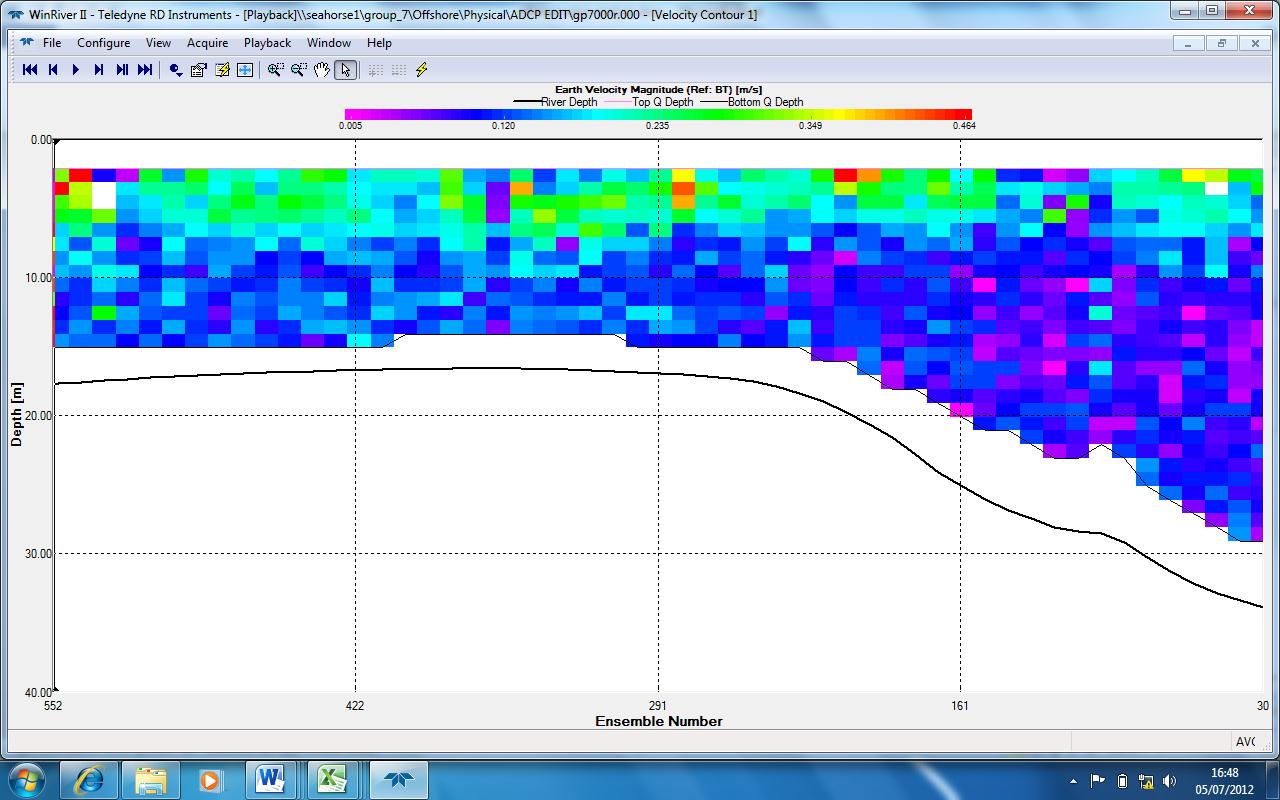
The velocity contour plot for station 3 on the estuary supports the relative Ri number of 11.93 with relatively uniform flow velocities throughout the water column reflecting stable conditions and hence a Ri number above 0.25. As well as this the velocity appears to increase with depth from 0.22m/s at 5.4m to 0.27m/s at 11.9m, which could result in the presence of shear however, the change in flow velocity is relatively small and will therefore limit the size of the shear. The increase in velocity with depth may represent the velocity of the tidal flow as the tidal flow is denser than the overlying riverine water, which would account for the increase in velocity with depth.
click to enlarge click to enlarge
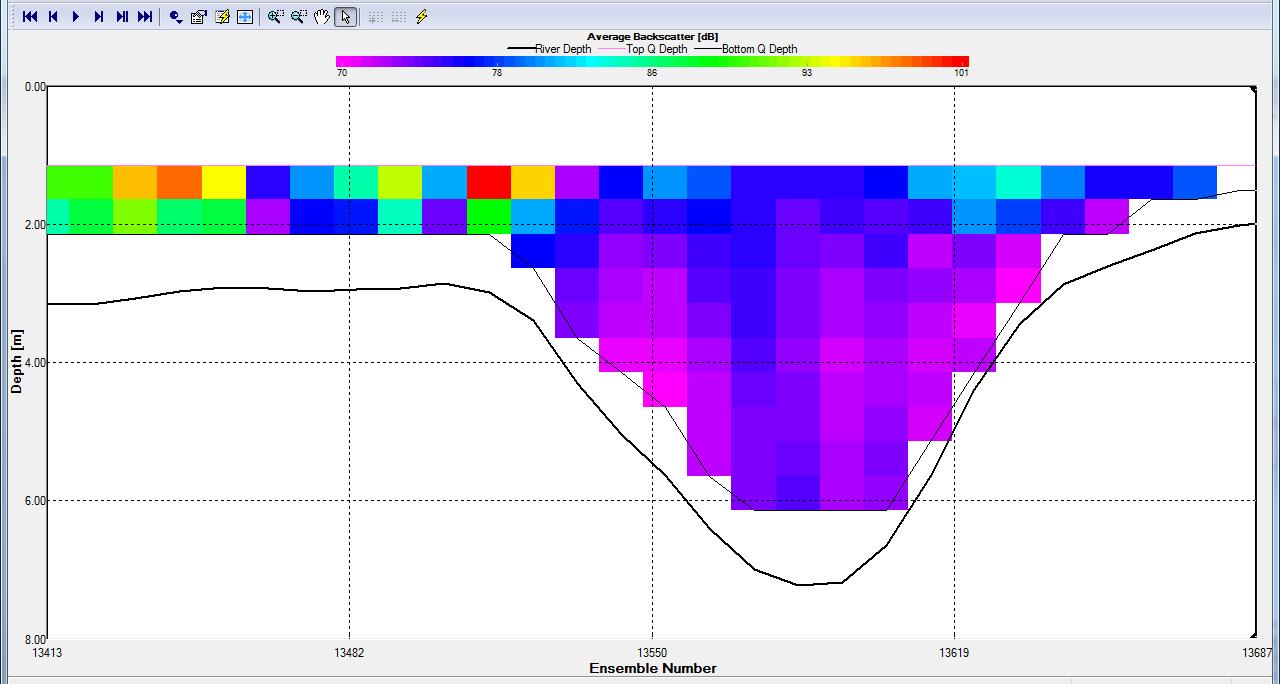
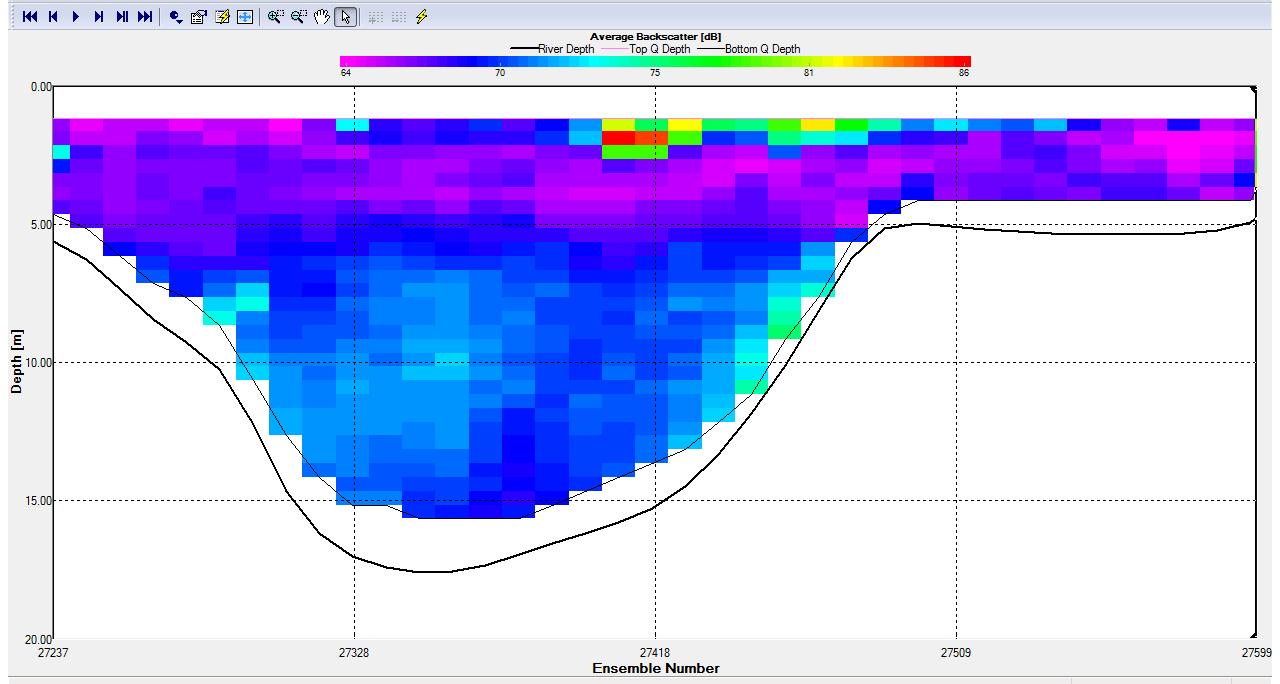
The ADCP estuary data consists of a large amount of noise and interference and therefore this can affect the accuracy of the Richardson results above.
Estuary conclusion The Fal estuary demonstrated the typical characteristics of a partially mixed estuary with thermal and haline stratification at all stations, this being most pronounced at the station in closest proximity to the freshwater input. The tidal currents affected physical properties, e.g. turbidity where the maximum was associated with the strongest current causing maximum shear at the water-sediment interface. The phytoplankton distribution reflected the light attenuation and declined logarithmically with depth. |
![]()
![]()
![]()
|
Introduction The water of the Western English Channel would be expected to be thermally stratified during summer months, this is caused by an increase in solar radiation. This controls the distribution and the abundance of planktonic organisms based on the chemical and physical structure of the water column (Kiorboe, 1993). The abundance and diversity of phytoplankton reflects the effects of their limiting factors namely nutrients and light intensity. Motility of species could also influence their density, as it allows migration between the euphotic zone which is nutrient poor with high light intensity, and the cold deep water beneath the thermocline which is euthropic with low light intensity. The density and abundance of zooplankton provides an indicator of the influence of predation on phytoplankton densities.
It is important to conduct investigations in attempt to understand the processes that contribute towards the variations in seasonal biological productivity. The main focus is to establish the rate at which nitrogen as nitrate and silicon as silicate can be mixed upwards across the thermocline.
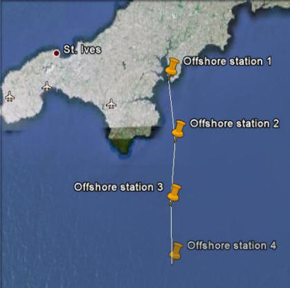
Method On board R.V. Callista, a predetermined transect was carried out where four stations were visited. These stations were as follows:
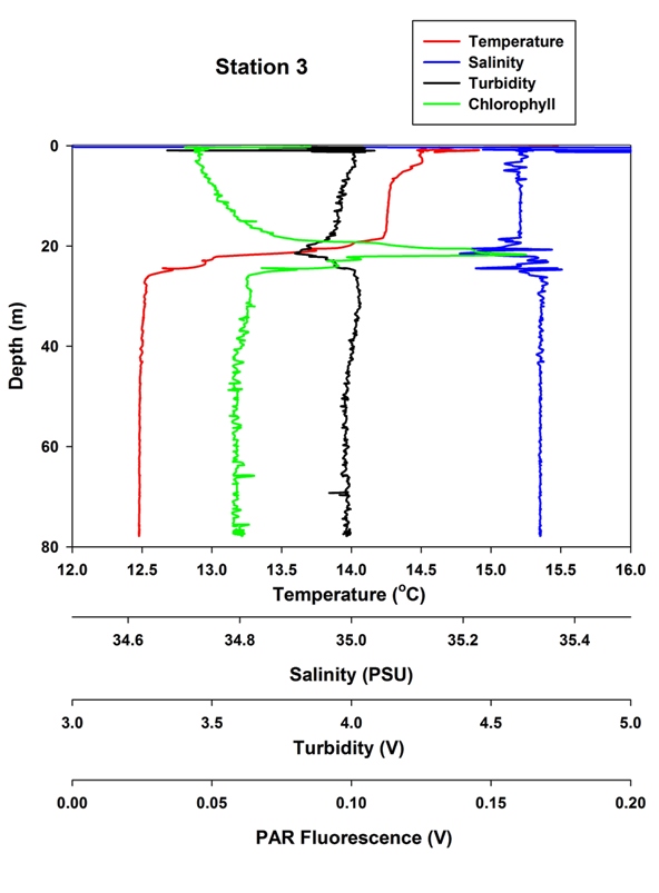
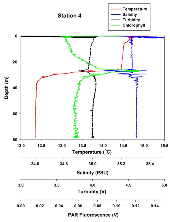
At each of these stations, maximum depth was noted and vertical profiles were drawn using a CTD, recording the following parameters; temperature, salinity, turbidity, irradiance and fluorescence (as a proxy for chlorophyll concentration). |
 |
 |
 |
 |
|
Station 1: This station was at Black Rock: in shallow (12m) water at the mouth of the estuary. As one would expect from a location so dominated by tidal mixing, turbidity and chlorophyll do not change. However, there is still evidence of river influence by way of a small halocline representing slightly reduced salinities (35) down to 5m where there is full strength seawater(35.2). A thermocline is also present between 3-7 metres, which represents the increased effects of riverine insolation. The low salinities observed in the first metre is most probably caused by heavy rainfall, and should be disregarded with reference to estuarine mixing.
|
Station 2 was 10 miles offshore in much deeper water (65m). The surface layer is thermally stratified, which is probably caused by seasonal variation in insolation. However, there is a well mixed intermediate layer down to 20m and a thermocline of around 1oc was observed as the CTD descended into a well-mixed bottom layer, where the temperature was constant down to the sea floor. Salinity was constant throughout the water column; the surface salinity spike is caused by a disparity between the rate of temperature change and the rate of salinity change. It is a feature of the CTD and should not be interpreted. The chlorophyll peak is actually above the thermocline, in the well mixed layer. However because of the stratification it still represents a biological optimum in regard to nutrients at depth and sunlight at the surface. Paradoxically, the water becomes clearer around the chlorophyll maximum/the thermocline. This is unexpected but may not be caused by biology and instead by a difference in SPM between the upper layer of water and the bottom layer.
|
Station 3 was 20 miles offshore and shows a textbook picture of 2 well mixed layers and a strong thermocline (2.5oc). As well, there is a chlorophyll maximum around the thermocline which represents a biological optimum between the nutrient rich bottom layer and the PAR-rich surface layer. In keeping with her chlorophyll maximum, beam transmission is decreased where there are more phytoplankton cells, more zooplankton cells, and more SPM due to messy feeding and excretions etc. |
Station 4 was 30 miles offshore and shows another classic picture of change with depth; the same thermocline seen at station 3 was observed, and the same increase in biology/decrease in beam transmission was also seen. There was a change in salinity between the 2 layers, albeit <0.1oc. This is just further evidence of 2 separate layers. |
![]()
![]()
![]()
|
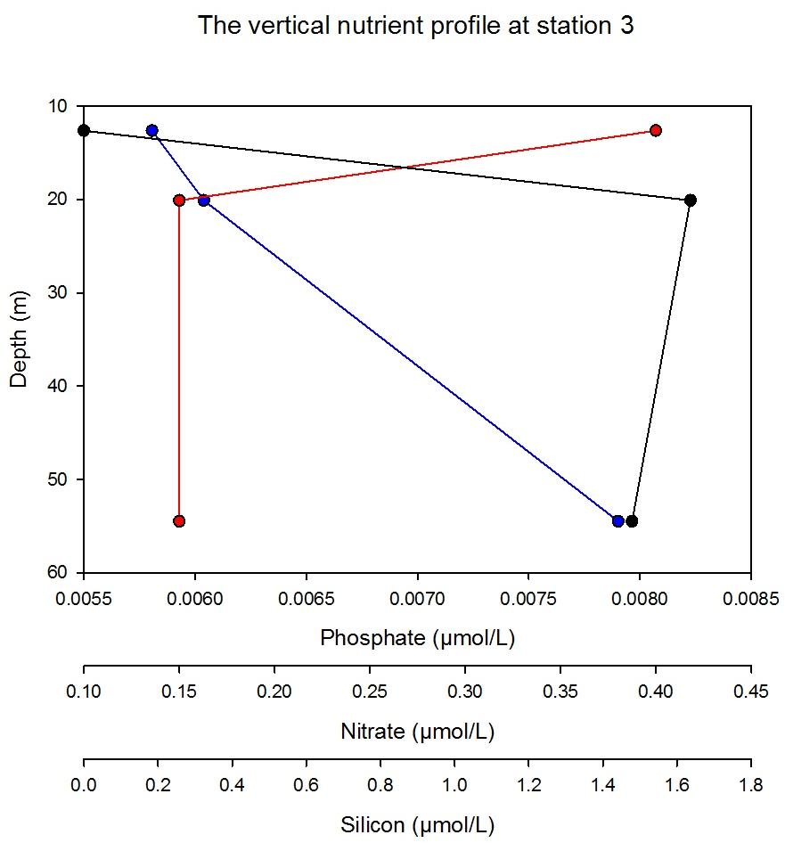
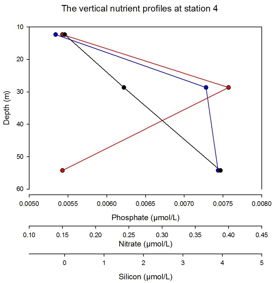
Nitrate (umol/l) |
Phosphate (umol/l) |
Silicon (umol/l) |
 |
 |
 |
 |
|
Oxygen Analysis Oxygen saturation (%) is used to indicate whether oxygen is being produced or consumed at a given depth in the water column. Factors controlling the saturation level are commonly photosynthesis and respiration, therefore oxygen levels are often linked to phytoplankton and zooplankton populations respectively. Values above 100% indicate a net O2 production and values less than 100% indicate consumption. click to enlarge
click to enlarge
click to enlarge
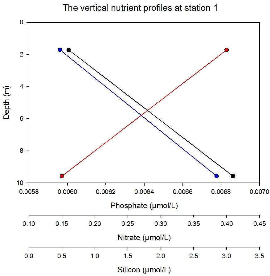
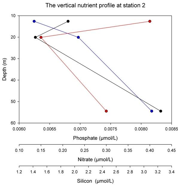
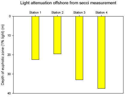
Phosphate At the sea surface phosphate is at around 6.0ug/l x 1000 and increases up to 7.0ug/l x 1000 in the upper 10 metres. However it then drops dramatically to between 5.0 and 5.5ug/l x 1000 at around 12metres. This drop could have been caused by initial phytoplankton blooms earlier in the year that occurred as the water became stratified. The phosphate stays at roughly 6.0ug/l x 1000 between 13 and 20 metres, where the thermocline begins. Then after the thermocline at 20m the phosphate level begins to gradually increase up to 7.5ug/l x 1000.The reason for this is the stratification of water. Phytoplankton in the warmer water, above the thermocline, have stripped the upper water of nutrients and have now moved down to the thermocline, just above the mixed lower water. They remove the phosphate from this region but the stratification stops phosphate rich water from mixing with the phosphate poor water. Phosphate shows the least variation and has the lowest concentrations of the three nutrients, but shows a consistent decrease with depth. Nitrate Nitrate was very low, below the detectable limit of 0.3μmol/L in 6 out of 11 samples. When considered in relative concentrations the nitrate appears to be the limiting nutrient on the growth of phytoplankton at these points. Silicon increases with depth at all stations except station 3 where the highest value is seen in the thermocline at 20.1m depth and at station 2 where the there is a decrease of 0.5 μmol/L between 12.6m and 20.1m. The equipment denied a meaningful insight into offshore nitrate levels as most of the samples did not have sufficient nitrate to facilitate accurate detection (detection limit of 0.03ug/l) Light The light penetration generally increased with distance from shore. Offshore, silts from turbid river waters have settled, so the euphotic zone is deeper. The exception to the trend is at station 2, with less light penetration, perhaps caused by high surface level phytoplankton densities in the water column, preventing the secci disk from being seen. The euphotic zone was below the thermocline at all stations, allowing photosynthesis at the boundary, causing the plankton densities found there; particularly further offshore, these stations had the greatest light penetration.
Plankton
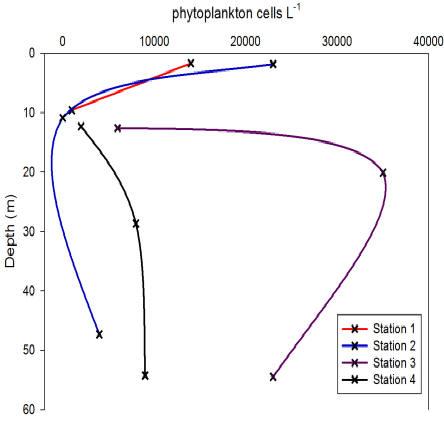
At near-shore stations such as station 1 (at the river mouth) and station 2 (10 miles offshore), phytoplankton growth was greatest at the surface. Here there is a far less pronounced thermocline. Conversely, at the further out stations, a noticeable thermocline can be measured, around which a chlorophyll maximum along with maximum phytoplankton densities (particularly at station 3). At the thermocline, light is still available, and nutrients just below are high. This allows large blooms to occur on the boundary.
Grazing these phytoplankton were large numbers of zooplankton. The highest densities corresponded with the surface bloom at station 2. This was dominated by copepods, which are grazed by notable numbers of chaetognaths, which prey upon them, along with the notable numbers of fish eggs; perhaps station two was near a fish nursery. Station 3 had much higher zooplankton levels at depth, with a trawl through the thermocline. Zooplankton typically remain just below the thermocline, to graze the phytoplankton above. Station 4 had fairly high concentrations of zooplankton towards the surface, despite phytoplankton counts here being comparatively low. The zooplankton may have grazed sufficiently to decrease the phytoplankton. Unfortunately, the sample from 40-20m was lost, so a comparison between surface and depth cannot be made.
Richardson Number
Station 1
There is a positive correlation between Ri number with depth. Ri is greater at the surface due to wind stress at the surface causing greater mixing. As depth increases the effect of wind decreases and consequently the water column becomes more stable, resulting in a difference in the speed of flow between the water layers and therefore the presence of shear.
Station 2
We would expect the greatest depth to have the largest Ri, however the greatest Ri was at a depth of 32 metres and had a value of 53.35. The fact the greatest Ri number is not at the greatest depth breaks from a trend of increasing Ri values with depth and could indicate slight turbulence in the water column at 57 metres. There is a positive correlation between Ri number and depth after 40 metres. Above 30 the Ri number is between 0.25 and 1.00 indicating shear flow. Wind moving across the surface of the water column results in a velocity change in the water column due to a large change in current shear as a result of wind on the air-sea interface. Station 3
At station 3 which was 49°49.785N, 005°00.691W and approximately 20 nautical miles south from Falmouth the maximum Ri was 1115 at a depth of 50.7 metres. The smallest Ri at station 3 was 0.008 at 2.5 metres. It is unsurprising that the Ri value near the surface is small because surface winds cause a velocity change within the water column this leads to change in velocity with depth and consequently shear. Unlike station 1 there is not an overall trend between depth and Ri. The Ri value at 35 metres is 274. This value has increased a large amount compared to all Ri values at higher depths; when the Ri graph for station 3 is compared to the CTD graph for the same location it indicates this depth is the start of the stable layer where wind no longer has an effect. The CTD graph for this location shows that after 35 metres there is little change in temperature, salinity and turbidity. This coupled with a high Ri which also illustrates no mixing means it is hightly probable this depth is the start of the stable layer in the water column Station 4
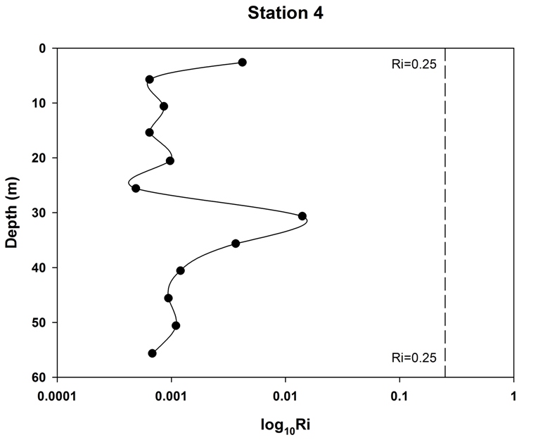
Station 4 which had latitude of 49°41.012N and a longitude of 005°00.583W was approximately 30 nautical miles south of Falmouth. We would assume at this exposed location the greatest influence on mixing was wind. The Ri number was calculated up to 55metre depths and the Ri value ranged between 0.47 at 2.6metres and 1 at 50.6metres. Because these values lie between 0.25 and 1 the stability of the water column cannot be determined however we would expect it to be stable. As depth increases wind has less of an affect and so the Ri values increase.
Station 1
Station 2
The average velocity of flow on the ship’s tracks increases from East to West with evidence of eddying at 75N and 18.4E.
Station 3
The ship’s track of station 3
indicates a flow with a relatively constant direction and velocity, with
the formation of ocean eddies at 89.2N, -290.1E.
Station 4
Conclusion The aim of our offshore investigation was to characterize the mixing system up to 30 miles south of Falmouth and therefore, identify any correlations in the following parameters; oxygen and chlorophyll concentration, nutrient activity and flow velocity. The oxygen samples collected indicate that when not affected by zooplankton and wind mixing oxygen saturation is dependent on the productivity of phytoplankton, supported by a strong correlation between chlorophyll concentration and oxygen saturation within the water column. Station 3 reflected the strongest correlation, whereas station 4 illustrated low oxygen saturation and hence high zooplankton density, possibly a response of surface wind mixing. With regards to ADCP data, station 1 indicates a decrease in velocity with depth as a result of bottom friction as the water column shallows. The depth of the water column increases to station 2 where velocity continues to decrease with depth, there is no apparent tidal affect. The flow velocity of the water column indicates greater tidal mixing at station 3 however, tidal mixing has a greater effect at station 4, where there is a clear boundary between the upper and lower water column. The velocity of the upper water column is controlled by wind mixing and overlies a faster moving water body controlled by the tides and hence, the velocity increases with depth. This is supported by Richardson numbers calculated from station 4, which reached a maximum value of 1, showing constant instability throughout the water column. Tides have less effect at station 3 as results were collected at 12:02 with a slack tide occurring at 12:03 and therefore, the tidal influence weakened. Estuarine dynamics are still influential on the water column properties of station 1 resulting in a shallow thermocline at approximately 3-7 metres and weak stratification due to freshwater riverine input and precipitation. The thermocline increases to 20-30 metres at station 2 due to a greater salinity gradient. The temperature gradient increases to 1.5oC at the thermocline for station 3, the depth of the thermocline remained fairly constant at approximately 30 metres through to station 4 however, the temperature gradient increased most likely due to solar warming reflecting a diurnal thermocline. With reference to nutrient concentrations there is no visible trend in Nitrate concentrations between the stations. We were therefore unable to calculate the Redfield ratio due to undetectable Nitrate concentrations. Unexpectedly low phytoplankton density, specifically diatoms, resulted in increased silicon concentrations within surface waters and a silicon maximum at the thermocline. |
|
Introduction The aim of this investigation was to survey the benthic habitat types within the Fal estuary and create a map based on the findings. The date of surveying was 02/07/2012. We experienced continuous rain on board the S.V Xplorer. High tide of 5.0m was at 15.55 GMT and low tide of 0.8m at 22.09 GMT. Only two transects were completed because of adverse conditions. Methods The initial intentions were to survey the estuary mouth to the east of Black Rock. However the poor weather conditions would have affected the detail of the Geoacoustics 159D sidescan and drop camera video footage, leading to increased interference in the data. The transect lines were therefore moved to the western, more sheltered, side of Black Rock. The rough weather also made it unsafe to launch the ROV at the first site because it requires calm conditions for safe steerage. The sidescan had a 75m swath width on either side and was towed behind S.V. Xplorer along the two transects within the estuary. This produced an image of the seabed which showed changes in bathymetry by recording the amount of backscatter; higher backscatter implies harder and more granular substrate. In order to accurately process the image, ground truthing was required in the form of two drop camera videos covering both transects. The course taken throughout this process was recorded to allow detailed analyses of collected data in the lab.
The sidescan showed 3 different zones within the survey area. These zones were identified as Zone 1: Macroalgae, Zone 2: Sand with ripple bedforms containing shells in the troughs and Zone 3: Shells with no clear bedforms. The natures of these zones were derived from the drop camera videos and the sidescan image. On the sidescan image the bedforms at zone 2 were not visible due to the angle of approach, therefore the bedform size cannot be calculated. The image did clearly show the macroalgae zone.
Zone 1 Zone 1 contains both red and brown macroalgae including species such as Laminaria digitata and Laminaria saccharina. Within the macroalgae are many other species of fauna and flora, such as bryozoa, anenomes and fish, including Labrus bergylta.
Zone 2 In zone 2 the seabed was is structured with ripples made up of sand, pebbles and shells. Due to the ripple direction and angle of transect direction approach, this structure was not seen clearly on the sidescan so the height and wavelength of these ripples cannot be estimated. The shells and larger pebbles were deposited in the troughs of these ripples. Zone 3 In zone 3 the seabed was made up of sand, pebbles and shells, however unlike zone 3 there were no bedforms or notable structures. This region was rich in Asterias rubens and there were also polycheate tubes. The shells were a mixture of species including: scallops and cockles.
Conclusion The fauna and flora changed noticeably between the zones. The ripples in zone 2 have very little flora or fauna, possibly due to the lack of shelter or solid, permanent anchoring points for flora and fauna. Meanwhile zone 1 is made up of a mix of red and brown macroalgae that offers itself as a home for a great number of species and is therefore an ideal nursery ground for several species. Zone 3 contained less macroalgae but had a high number of A. rubens.
There were no maerl beds seen within the survey region despite this region containing some of the only maerl beds in the UK. Maerl beds are of high importance within the Fal estuary, due to the habitat they provide, as a structure to specific species, along with juvenile fish. Whilst planned dredging may have a detrimental impact upon these maerl beds, the transect area surveyed is unlikely to be too significantly affected by an influx of silt. However more surveying should be done to identify the more sensitive habitats, and gauge the overall consequences of dredging. |
Click the image to enlarge the electronic poster

Click to load the videos (Large Files)
|
BlackBoard, Coastal And Estuarine 1 Soes2025, course information, estuarine flushing lecture Bryan and Langston, 1992, ‘Bioavailability, accumulation and effects of heavy metals in sediments with special reference to United Kingdom estuaries – a review.’, Environmental Pollution, 76, 89-131 CEH 2012, [Online] Available:http://www.ceh.ac.uk/data/nrfa/ [Accessed 5th July 2012] Accessed from 26th June to 6th July: Google Earth 6.0.3.2197, Google, 5/17/2011
Hawkins and S. J. 2006, ‘ Characterisation of the European Marine Sites in South West England: the Fal and Helford candidate Special Area of Conservation (cSAC) .’, Hydrobiologia, 555, 321-333. Hosking, K. F. G. and Obial, R. 1996, ‘A preliminary study of the distribution of certain metals of economic interest in the sediments and waters of the Carrick Roads (West Cornwall) and of its feeder rivers.’, Cambourne School of Mines Magazine, 17-36. Kiorboe, 1993 Turbulence, phytoplankton cell, cell size and the structure of pelagic foodwebs. Advanced Marine Biology, 29, 1-67 Kraberg, A., Beumann, M. and Dürselen, C. D. 2010, 'Coastal Phytoplankton', Verlag Dr. Friedreich Pfiel, München Germany. Langston, W. J., Chesman, B. S., Burt, G. R., Taylor, M., Covey, R., Cunningham, N., Jonas, P., Hawkins and S. J. 2006, ‘ Characterisation of the European Marine Sites in South West England: the Fal and Helford candidate Special Area of Conservation (cSAC) .’, Hydrobiologia, 555, 321-333. Langston, W. J., Chesman, B. S., Burt, G. R., Hawkins, S. J., Readman, J. and Worsfold, P. 2003 Larink, O. and Westherde, V. 2006, 'Coastal Plankton Photoguide for European Seas', Verlag Dr. Friedreich Pfiel, München Germany. Accessed: http://www.licor.com/env/products/light/ 26th June 2012 Marsh, T. J. and Hannaford, J. (Eds). 2008. UK Hydrometric Register. Hydrological data UK series. Centre for Ecology &Hydrology. 210 pp. Maier, G., Nimmo-Smith, R. J., Glegg, G. A., Tappin, A. D. and Worsfold, P. J. 2008, ‘Estuarine eutrophication in the UK: current incidence and future trends.’, Aquatic Conservation: Marine and Freshwater Ecosystems, 19, 1, 43-56. Accessed: www.mba.ac.uk/nmbl/publications/charpub/pdf/Fal_Helford.pdf , 5th July 2012 Accessed: www.metoffice.gov.uk 6th July 2012 Accessed: http://nora.nerc.ac.uk/3093/1/HydrometricRegister_Final_WithCovers.pdf 5th July 2012 Pirrie et at (1995). Mineralogical and Geochemical Signiture of Mine Waste Contamination, Tresillian River, Fal Estuary, Cornwall, UK. Environmental Geology. Vol 29 Ed:1-2 pp58-65 Accessed: http://www.rdinstruments.com/mm_products.aspx 26th June 2012 Strickland, J. D. H. & Parsons, T. R. 1968, 'Determination of Reactive Silicate', A practical handbook of seawater analysis, Fisheries Research Board of Canada. Accessed: http://www.southampton.ac.uk/assets/imported/transforms/peripheral-block/UsefulDownloads_Download/9E7194EF55094B379817B2EB20545CDD/B_Conway.pdf 30th June 2012 Accessed: http://www.southampton.ac.uk/discoveroceanography/rv_callista/ 30th June 2012 Accessed: http://www.southampton.ac.uk/oes/research/facilities/research_vessels/conway.page 30th June 2012 Accessed: http://www.valeport.co.uk/Products/CurrentMeters.aspx 26th June 2012 Accessed: http://www.ysi.com/productsdetail.php?6600V2-1 26th June 2012 United Kingdom Hydrographic Office 2008 [Online] Availiable: http://www.ukho.gov.uk/Pages/Home.aspx [Accessed 27th June 2012]
Disclaimer All views and opinions expressed are those of the individuals involved in this project and are not representative of the University of Southampton or its staff. |
 The
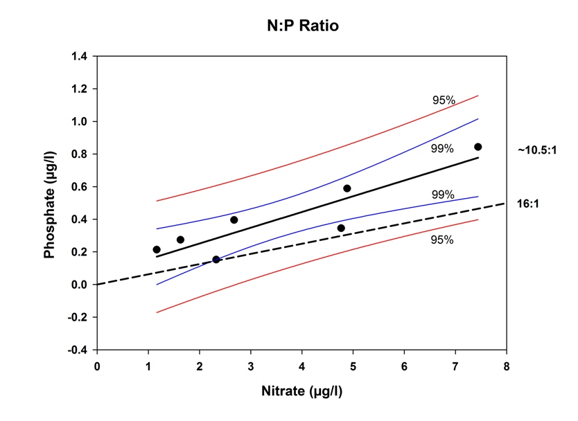
graph to the right compares nitrogen and phosphate data from
the estuary. The black regression line shows strong correlation (r2=0.81)
and the coloured lines either side of it show a 99% and 95% confidence
band. The black dotted line represents the Redfield ratio of 16:1, which
passes through the confidence limits of our observed N:P regression.
This shows that while an N:P ratio of 10.5 is seemingly different from a
Redfield ratio of 16, in the case of this dataset at least there is no
statistically significant difference between the observed N:P ratio and
the Redfield ratio.
The
graph to the right compares nitrogen and phosphate data from
the estuary. The black regression line shows strong correlation (r2=0.81)
and the coloured lines either side of it show a 99% and 95% confidence
band. The black dotted line represents the Redfield ratio of 16:1, which
passes through the confidence limits of our observed N:P regression.
This shows that while an N:P ratio of 10.5 is seemingly different from a
Redfield ratio of 16, in the case of this dataset at least there is no
statistically significant difference between the observed N:P ratio and
the Redfield ratio.
 The
phytoplankton structure at all stations measured was dominated by
diatoms. These are able to bloom in spring, before the nutrients are
depleted; notably silicate which they utilise within the frustule. With
unseasonably cold wet weather, this spring growth may have been pushed
back to early summer.
The
phytoplankton structure at all stations measured was dominated by
diatoms. These are able to bloom in spring, before the nutrients are
depleted; notably silicate which they utilise within the frustule. With
unseasonably cold wet weather, this spring growth may have been pushed
back to early summer.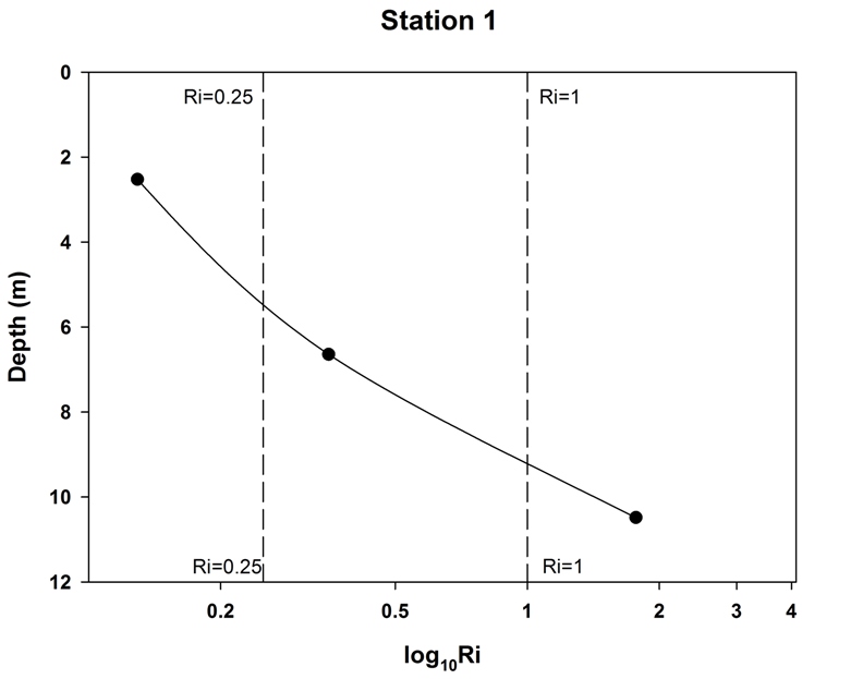 Station
1 which was adjacent to Black Rock shows an increase in the Richardson
number (Ri) with depth. At a depth of 2.53metres Ri
has a value of 0.129, 6.64metres has an Ri value of
0.35. The geatest depth at which Ri was calculated for
station 1 was 10.48metres had an Ri value of 1.76. At 2.53
metres there is instability of the water column which causes shear flow
and a Ri value below. 0.25. The measurements at 10.48 metres
is both greater than 1 and indicates a stable flow with no mixing.
Station
1 which was adjacent to Black Rock shows an increase in the Richardson
number (Ri) with depth. At a depth of 2.53metres Ri
has a value of 0.129, 6.64metres has an Ri value of
0.35. The geatest depth at which Ri was calculated for
station 1 was 10.48metres had an Ri value of 1.76. At 2.53
metres there is instability of the water column which causes shear flow
and a Ri value below. 0.25. The measurements at 10.48 metres
is both greater than 1 and indicates a stable flow with no mixing.
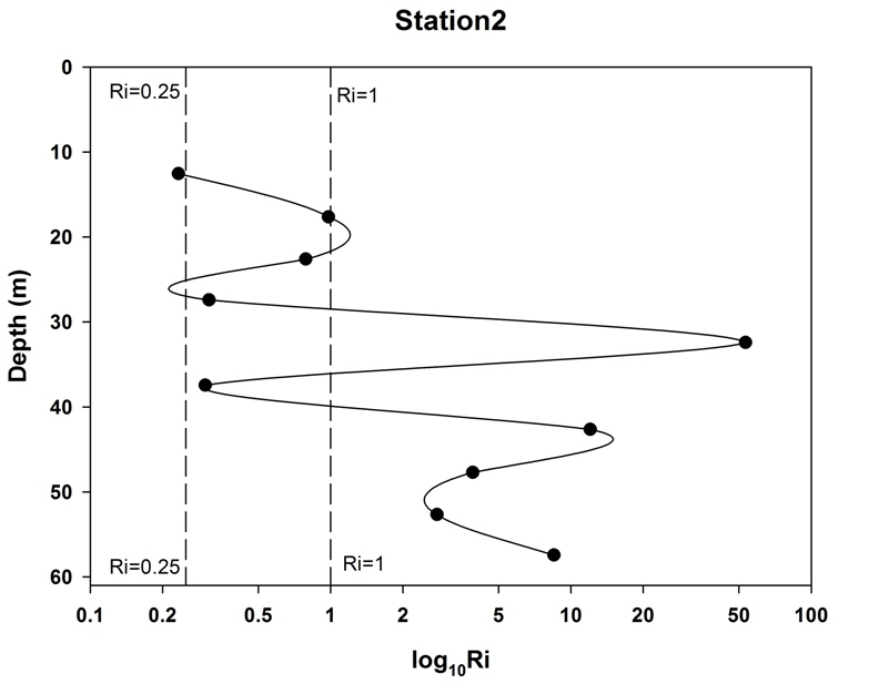 Station
2 which had latitude of 49°59.314N and a longitude of 004°59.849W was
approximately 10 nautical miles south of Falmouth. The Richardson number
was calculated for 10 different depths between 12 and 57 metres. The
smallest Ri was 0.23 and at a depth of 12 metres, this
indicates instability and shear flow between water layers
Station
2 which had latitude of 49°59.314N and a longitude of 004°59.849W was
approximately 10 nautical miles south of Falmouth. The Richardson number
was calculated for 10 different depths between 12 and 57 metres. The
smallest Ri was 0.23 and at a depth of 12 metres, this
indicates instability and shear flow between water layers