|
FALMOUTH FIELD COURSE GROUP 6 |
 |
|


|
|
Who Are We?
...5
Oceanographers...
...5 Marine
Biologists...
From left to right:
Tommaso Bendoni, George
Grant, Lisa Holton,
Matt
Hawksworth, Rachel Cook, Sam Gill, Becci Owen,
TJ Kearney, Ellie
Hoolahan, Emily Last |
 |
|
Figure 1. Simple overview map of Falmouth and its surroundings |
Introduction
An investigation into the
biological, chemical and physical processes in the Fal Estuary in
Cornwall, England (see Figure 1) was carried out from the 26th
of June to the 6th of July. Observations were made in three
primary sessions, on research vessels, around the estuary and consisted
of an ‘Offshore’, an ‘Estuarine’ and a ‘Geophysical’ investigation.
The Fal estuary can be
geomorphically classified as a classic ‘Ria’, or drowned river valley,
and is thought to have been formed from the beginning of the Holocene as
a result of sea level rise (Langston et al, 2003). The Fal Estuary forms
part of the Carrick Roads, which is the deepest natural harbour in the
world, with a maximum depth of 35 m (Langston et al, 2003). These types
of estuaries are usually large shallow inlets and bays, and the diluting
effects from freshwater inputs are minimal. The harbour is subject to
many anthropogenic, industrial and recreational pressure, such as
dredging, sewage inputs, mining and industrial runoff.
The Fal Estuary is affected by
south-westerly Atlantic winds and experiences macrotidal conditions at
the mouth (Falmouth), with a maximum spring tide of 5.3m, and mesotidal
conditions at the head (Truro) with a maximum spring tide of 3.5m
(Pirrie et al, 2003).
The west of the estuary is
surrounded predominantly by Carnmellis granite and other metamorphic
rock. The large input of China clay waste from St Austell has a major
silting impact on the upper estuary and the salt marshes (Langston et
al, 2003). The Fal is a designated special area of conservation and is a
site of protected habitats such as maerl and seagrass beds as it is the
site of many habitats such as maerl beds.
The area has a substantial
history of mining, peaking in the 19th century. Much of the
tailings and wastage were deposited in Restronguet Creek, resulting in
the highest concentration of polluting metals found in the UK (Langston
et al., 2003). |
|
Schedule
|
Date |
Activity |
|
26/06/12 |
Web
Preparation (am)
Pontoon (pm) |
|
27/06/12 |
Data |
|
28/06/12 |
Offshore Boat
Practical |
|
29/06/12 |
Offshore Lab
Practical |
|
30/06/12 |
Data |
|
01/07/12 |
|
|
02/07/12 |
Geophysical
Boat Practical |
|
03/07/12 |
Geophysical
Lab Practical |
|
04/07/12 |
Estuary Boat
Practical |
|
05/07/12 |
Estuary Lab
Practical |
|
06/07/12 |
Data and
Finish |
|
|
Equipment |
|
CTD
The CTD is deployed using a hydraulic winch from the rear of the
boats where it is used to continuously measure the parameters
conductivity, temperature and depth. Using the electrical
conductivity of the seawater, salinity can be measured. The CTD
provides real time, high-resolution data via the electrical
cable powering the device. In context here, it is used in
conjunction with a rosette sampler and other systems on a
mounted frame. The CTD was used both in the estuary and offshore
to measure depth, temperature and salinity of the water column.
|
Equip 1. CTD in operation |
|
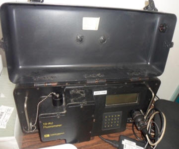
Fluorometer
The fluorometer is part of the CTD Rosette system, and also as a
way of analysing samples in the laboratory. It measures the
fluorescence of the water around it by sending out a known
wavelength of light and measuring the returning wavelength of
light and its corresponding intensity. It was used as a
standalone instrument in the lab to analyse chlorophyll samples
and also in situ as part of the CTD setup.
|
Equip
2. Laboratory Fluorometer |
|
|
Transmissometer
The transmissometer is also part of the CTD Rosette system. It
measures the attenuation of a known light source to calculate
the turbidity of the seawater, producing results in
nephelometric turbidity units (NTU). The transmissometer was
part of the CTD setup and was used primarily offshore.
|
ADCP
The Acoustic Doppler Current Profiler is an instrument that is
attached to the hull of the boat and connected to a computer in
the labs on board the boat. It sends out pulses of sound and
measures the doppler shift, a shift in frequency of the sound
emitted and the resulting returning sound; caused by the
differing velocities in the water column. The constant pulses
allow real time readouts of the structure of the water column to
be displayed and the differing colours on the readout allow easy
interpretation. The ADCP was used during the estuarine, offshore
and geophysical work to provide real time data of the water
column.
|
|
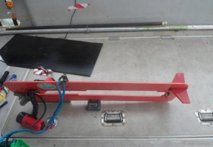
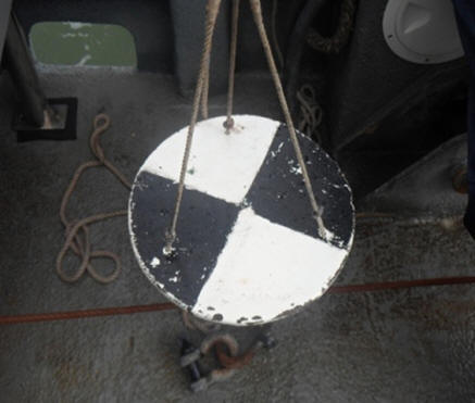
Secchi Disk
The
Secchi disk is a circular plate with the pattern as shown in the
picture. It is attached to a rope and lowered into the water
until it can no longer be seen. When this depth is measured and
recorded, the light attenuation coefficient can be calculated.
This can be used to estimate the depth of the euphotic zone; 3
times the depth of the Secchi depth. The secchi disk was only
used in the estuary as the light meter was not part of the CTD
setup on the Bill Conway.
|
Equip 3. Secchi Disk on board RV Bill Conway |
|
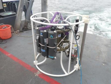
Niskin Bottles
Niskin bottles are hollowed tubes attached to a hydrographic
line, which can be ‘fired’ from on deck with a weighted
messenger, causing caps to spring closed at both ends. Water can
freely flow through the tube until the caps are closed, reducing
the possibility of surface contamination. Multiple bottles are
set up in the rosette sampler. These were used on the offshore
trip as part of a rosette system and during the estuarine work
whilst attached to a hydroline to collect relevant samples
|
Equip 4. Niskin Bottles on Rosette System |
|
YSI Probe
The YSI probe was deploymed from the pontoon and then used to
create a vertical transect of water body characteristics. With
the probe, it is possible to measure depth (m), temperature
(°C), salinity (psu), pH, chlorophyll (μg/l) and dissolved O2
(%).
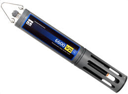
Equip 5. YSI Probe
|
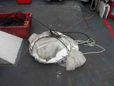
Closing Net
This is a weighted net that sits vertically in the water
column. A plastic bottle is attached to the bottom of the net
in which a water sample can be collected as the net is raised
through the water column. A messenger is released down the
connecting line, closing the mouth of the net and allowing the
particulate matter in the net to settle out into the bottle.
The net used for plankton collection has a 200 μm fine mesh, and
mouth diameter of 0.6m. This net was used offshore to collect
water samples in a closed bottle for analysis of the
phytoplankton and zooplankton content. A similar net was used
during estuarine work but it could not closed, so it was used
during a plankton trawl at a set depth.
|
Equip 5. Phytoplankton and Zooplankton collection |
|
|
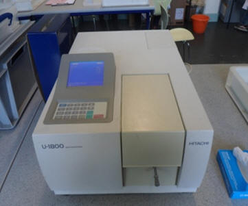
Spectrophotometer
The spectrophotometer measures the absorbance of light within a
fluid. A ray of light is passed through the fluid sample, and a
detector consequently measures the amount of light that passes
through the entire sample. When comparing the absorbance of a
given sample against a calibration curve, produced from a set of
known standards, the concentrations of chemicals within the
fluid sample can be obtained. This apparatus was only available
in the lab to analyse samples as it is not part of any in situ
sampling equipment. Most samples put through this need to be
treated first.
|
Equip
6. Laboratory Spectrophotometer |
|
|
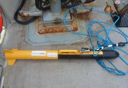
Side-Scan Sonar
The side-scan sonar is towed behind the vessel emitting a fan
shaped sonar beam down through the water column. The time taken
for the pulse to return to the detector allows an image of the
seabed to be formed. Upon analysis of the data, this image can
be used to determine the size and shape of objects on the sea
floor and to determine sediment structure and content. The
side-scan sonar was used during geophysical work to create the
habitat map of the riverine transect and to locate associated
features.
|
Equip 7.
Side-Scan Sonar Operational Apparatus
|
|
Video Camera
Depth
controlled precision video camera, with light, used for ground-truthing
over the side of the Xplorer. It is important to ensure that the
camera does not touch the sea bed, yet must be at a suitable
height to collect accurate images of the bed. Care should be
taken in this instance. Linked by electronic cable back to
real-time a monitor on board the vessel, where images can be
saved to a DVD disk for later viewing and analysis. This was
only used during geophysical work to provide shots of the seabed
for analysis that would correspond to the habitat map.
|
Equip 8.
Operational Video Camera |
|
Hydroline
The
hydroline was used on the RV Bill Conway for deployment of a
Niskin bottle, concerned with the collection of water samples
for laboratory analysis - oxygen, chlorophyll, nitrate,
phosphate, silicon contents. The hydroline is a reinforced
thick cable with a Niskin bottle clamped to it, attached to a
manual winching system. When the winch is operated, further
length of cable is wound down into the water below and the
Niskin bottle fills. A messenger is released by hand at the top
of the hydroline to seal off the ends of the bottle and the
cable, with attached Niskin, can be wound back onto the boat.
|
|
Research Vessels |
R.V. Bill Conway
We used the Bill Conway vessel for the estuarine analysis
work, including the deployment of analytical instruments.
Bill Conway is a 12m single hull research vessel built for
inshore water sampling and surveying. A small dry lab plus
the covered rear deck provide space for analyses with a
winch and 2 davits for equipment deployment.
For more web-based information,
click here.
Specifications:
Length: 11.74m
Breadth:
3.96m
Draft: 1.30m
Max Speed: 10 knots
Range: 150 Nautical Miles
Max Passengers: 12 + 2 crew
Equipment:
A-Frame - 750kg limit
2 side davits - 50 kg
limit
|
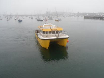
R.V. Callista
We used the Callista vessel for the offshore analysis work,
including the deployment of analytical instruments and the
vessel's own laboratory and IT services. R.V Callista is a
purpose built 19.75m twin hulled catamaran, with the ability to
conduct research of coastal and shelf seas up to 60 miles
offshore. A large flat rear deck features an A frame and winch
with 4 tonne lifting capacity for equipment deployment. On
board, wet and dry labs allow in-situ processing and analyses of
data.
For more web-based information,
click here.
Specifications:
Length: 19.75m
Breadth: 7.40m
Draft: 1.80m
Max Speed: 15 knots
Range: 400 Nautical Miles
Max Passengers: 30 + 4 crew
Equipment:
ADCP
CTD Rosette
Digital Thermosalinograph
Flurorometer
Transmissometer
|
SV Xplorer
We used the Xplorer for the geophysical analysis work, including
the deployment of the side-scan sonar and video camera, thus
enabling us to later create a habitat map in the laboratory. The
SV Xplorer is a twin hulled research vessel with specialist
adaptions for dive supported research. Stern door and large rear
deck with winch for equipment deployment. A dry lab area with
computer access provides live data feeds for in-situ analyses
and processing.
Specifications:
Length overall: 12.00m
Breadth: 5.20m
Draft: 1.20m
Max Speed: 25 knots
Max passengers: 14 + 3 crew
Equipment:
1 tonne hydraulic crane
Side-Scan Sonar
ADCP
Van Veen grab, Plankton Nets
CTD, Niskin Bottles
|
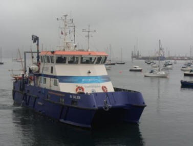
Equip 9. RV Callista before Offshore work commenced
|
|
Equip 10. SV Xplorer before Geophysical work |
|
|


 |
|
Offshore Work - RV
Callista (28/06/2012) |
|
|
Date |
28/06/2012 |
|
General Weather |
Overcast |
|
Visibility |
Poor |
|
Sea State |
Rough |
|
Cloud Cover |
8/8 morning 6/8 afternoon |
Tables 1 and 2. Meteorological data and tide times
for offshore work
|
28/06/2011 |
Tide Times GMT |
Tidal Height (m) |
|
Low Water |
0629 |
1.30 |
|
High Water |
1226 |
4.40 |
|
Low Water |
1857 |
1.40 |
|
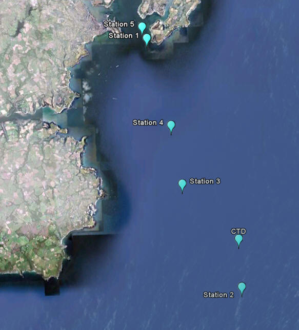
Figure 2.
Transect map for Offshore Stations |
|
Abstract/Background
The aim of this
investigation is to determine how vertical mixing processes in the
coastal waters of the English Channel off Falmouth affect, directly and
indirectly, the structural and functional properties of plankton
communities.
Vertical mixing has a
profound influence on the properties of the surface layer, which largely
controls the planktonic productivity and distribution (Kiorboe, 1993).
This investigation was carried out in the summer months (June), when the
surface waters tend to be nutrient depleted and the deep waters are
nutrient rich and therefore will focus on the rate at which nitrate and
silicate can be mixed upwards across the thermocline. This occurs as
there are lower rates of surface mixing and higher irradiance levels in
the summer months. Fronts form in the regions where the well mixed,
nutrient rich coastal waters meet the well stratified waters.
Planktonic productivity is high in this region due to the abundance of
nutrients found along these frontal systems. Nitrate is an essential
nutrient required by all types of phytoplankton and silicate is required
specifically by diatoms for growth and formation of their siliceous
skeletons.
Data was collected from stations listed in the table below. A
full sample included a CTD cast to obtain physical measurements, sample
collection in order to determine chemical properties such as nutrient
and dissolved oxygen levels. The
CTD was deployed from the back of RV Callista and was lowered down to
the required depths via a winch system. It contained a temperature and
salinity probe, light sensor, fluorometer and a series of Niskin bottles
on the Rosette sampler which collected the water samples. These samples
were used to obtain the dissolved oxygen, chlorophyll, silicon, nitrate
and phosphate data, and were stored in smaller glass bottles, apart from
the silicon ones which were put into plastic bottles, ready to be
transferred to the lab for analysis. It is unfeasible to put any samples
for nitrate and phosphate analysis into plastic bottles because they are
made of organic materials, which may contaminate samples, thus providing
inaccurate results. Glass contains silica, so can therefore not be used
to contain the dissolved silicon samples, as the eventual silicate
concentrations were analysed in the laboratory.
Biological data was obtained through phytoplankton and
zooplankton sampling, using a closing net with mesh size 200µm. This was
deployed via a winch from the back of Callista, and lowered to depths
defined on the CTD fluorometer and ADCP data as being significant. It
was raised over the pre-defined depth range, for example from 30m to
20m, and then closed via messenger weights. The water samples collected
in the 500ml bottle attached to the bottom of the net were then placed
in plastic containers for consequent identification in the laboratory.
The ADCP is permanently on the hull of Callista, and so was switched on
at the beginning of the survey. Therefore the velocity and direction of
the current was recorded over the entire survey time, enabling the
creation of horizontal profiles.
Two survey routes were
planned in order to allow for weather interferences. Plan A was to be
carried out if the weather was suitable, which would involve RV Callista
travelling straight outwards from the coastline in a south easterly
direction. Plan B would involve RV Callista travelling along the coast
in the shelter of Lizard Point, as this would still allow the
investigation to be carried out if conditions were unsuitable for work
further offshore, for example with the presence of extreme fog. Plan A
was carried out, and an overview of the route is listed in Table 3
below.
|
Station Number |
Latitude
(WG584) |
Longitude (WG584) |
Time
(UTC) |
Activity |
|
1 – Black Rock |
50°08.241N |
005°01.225W |
0945 |
Full sample station |
|
2 |
49°59.561N |
004°56.071W |
1051 |
Full sample station |
|
3 |
50°03.169N |
004°59.306W |
1143 |
Full sample station |
|
4 |
50°05.220N |
004°59.913W |
1342 |
Full sample station |
|
5 |
50°08.701N |
005°01.500W |
1456 |
Full sample station |
|
Surprise CTD |
50°01.217N |
004°56.220W |
1152 |
CTD cast only |
Table
3. Positions
and details of offshore sampling stations
Chemical Analyses
|
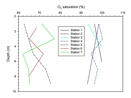
At almost all sampling stations,
oxygen is oversaturated. It is only in the very deep water that the
oxygen is undersaturated. In the surface waters, especially at station
1, the oversaturation can be attributed to biological activity within
the water column, suggesting the presence of photosynthetic organisms
such as phytoplankton outweighing the effect of microbial respiration.
The deeper water samples that were undersaturated are likely to exist
below the compensation depth, leading to a gradual reduction in the O2
saturation.
The very high saturation at station 1 may correspond
with nutrient rich fresh water and strong tidal and wind mixing;
therefore keeping oxygen and nutrient concentrations high (McKinney,
2004). This allows for excessive phytoplankton growth in the estuarine
surface layers. The similar peak at station 3 is at a greater depth,
which corresponds with a deep-water chlorophyll maximum (Weston et al.,
2005). The stratification parameters support this as deep-water
chlorophyll maxima are expected in stratified areas and in shelf seas (Holligan
et al., 1984). |
Figure 3. Oxygen
Saturation Depth Profiles
 |
During
nitrate analysis, pre-existing standards were used that were known to be
accurate and correctly made up. From these peaks, we were able to
calculate the relative amount of nitrate in our samples of seawater.
Three stations were tested at different points along the offshore data
sampling, allowing us an effective cross section from the mouth of the
estuary, right out to our furthest sampling point offshore at station 2.
The majority of samples contained very little nitrate, below the
detection limit of the apparatus. This was to be expected from the high
salinities present in all of our samples. Only one sample that had a
measurable nitrate concentration was from station 3. This sample only
just had peaks that were repeatable and also measurable, but they also
confirm what was expected, for nitrate to be very low in offshore
environments. It was surprising however, as it wasn’t our lowest
salinity value, but one of our highest. Surface mixing and variable
light over the previous few days will have lead to local variation.
Table 4. Nitrate
results and corresponding relevant information during the analysis stage
|
Station |
Lat |
Long |
Depth (m) |
Salinity (psu) |
Bottle No. |
Nitrate (μM) |
|
Standard |
Standard |
Standard |
N/A |
N/A |
Standard |
10 |
|
3 |
50°03.169 |
004°59.306 |
0.874 |
35.346 |
51 |
Below Detection |
|
3 |
50°03.169 |
004°59.306 |
14.543 |
35.251 |
45 |
Below Detection |
|
3 |
50°03.169 |
004°59.306 |
41.109 |
35.244 |
20 |
0.714 |
|
3 |
50°03.169 |
004°59.306 |
20.913 |
35.194 |
6 |
Below Detection |
|
2 |
49°59.561 |
004°56.071 |
60.606 |
35.344 |
56 |
Below Detection |
|
2 |
49°59.561 |
004°56.071 |
26.325 |
35.286 |
55 |
Below Detection |
|
2 |
49°59.561 |
004°56.071 |
0.826 |
35.203 |
54 |
Below Detection |
|
5 |
50°08.701 |
005°01.500 |
24.8 |
35.183 |
50 |
Below Detection |
|
5 |
50°08.701 |
005°01.500 |
11.1 |
35.102 |
48 |
Below Detection |
|
5 |
50°08.701 |
005°01.500 |
0.811 |
34.724 |
7 |
Below Detection |
|
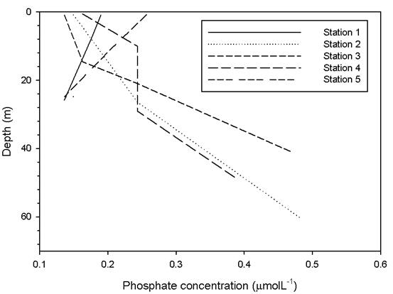
When analysing samples for their phosphate contents, it is important
to remember that stations 1 and 5 were both taken at Black Rock at
50o 08.214N and 005o 01.225W at the mouth of
the estuary, but were taken at different times. The samples for
station 1 were taken at 09:05-09:41 UTC, whereas the samples for
station 5 were taken at 14:56-15:01UTC. As a result of this, the
same site was sampled at differing times in the tidal cycle. This
may explain why an increase in phosphate concentration was seen when
the Black Rock site was sampled for a second time. With the tide
starting to fall when the samples from station 5 were collected,
water with higher phosphate concentrations will have been entering
the system from the estuary. The influence of nutrient rich fresh
water explains the high surface concentrations of phosphate, and as
Black Rock is relatively shallow, the whole water column will be
tidally mixed and well lit providing suitable conditions for algal
growth leading to the concentrations decreasing with depth.
Station 2 shows increasing concentrations of phosphate with
increasing depth, with the maximum concentration being seen at 60m.
Stations 3 and 4 also show decreasing concentrations with depth,
with maximums at each station occurring at the deepest depth
sampled. The station does however show an area of mixed water
between 10-30 metres, and this is also seen when looking at the CTD
casts for this station.
|
Figure 4. Phosphate concentrations for all five stations plotted
against depth. Stations 1 and 5 show decreasing concentrations in
phosphate with depth. Stations 2-4 all show increasing
concentrations with depth.
 |
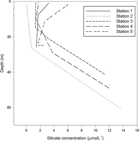
Again as in the phosphate figure, it is important to bear in mind
for the silicate measurements that both stations 1 and 5 are taken
at Black Rock at differing times in the tidal cycle. The samples
taken at station 1 were collected towards high tide, whereas the
samples from station 5 were collected as the tide was falling. This
has yielded silicate results similar to the phosphate profiles, with
station 5 having higher concentrations at all depths when compared
to station 1. The reasoning for the increased concentrations, is the
result of nutrient rich freshwater entering the marine system from
the estuary. The trend of decreasing concentrations at both
stations 1 and 5 are due to Black Rock being in a tidally mixed body
of water provides enhanced conditions for phytoplankton growth, and
this coupled with the Black Rock being relatively shallow and well
lit leads to the continued uptake of nutrients at depth.
|
The samples collected at stations 2 and 3 show an increase in the
concentration of silicate with depth, which is to be expected as
both stations are from stratified waters. Although station 2 shows a
slight increase with depth hinting at a relatively large mixed
layer, station 3 has a very small stable layer extending down to
about 16m and the silicate concentrations increase with
depth.
Station 4 has a slightly unusual profile, as for the first 15m, the
silicate concentrations decrease with depth. This is more than
likely due to phytoplankton activity. From around 15m to 28m there
is a slight increase seen in the concentration of silicate and then
from 28m until the deepest sample taken, the concentrations
increase. This unusual behavior may be the result of a number of
different water bodies mixing at this station, supported by the fact
that this irregularity is also seen in the depth profiles generated
from the CTD casts at this station.
Figure 5. Silicate concentrations for all five stations against
depth. Stations 1 and 5 show higher silicate concentrations at the
surface when compared with depth. The plateau seen in station 5 at
the maximum depth is as a result of replicates being carried out
with differing values being generated. For stations 2 and 3
increases in silicate can be seen with increasing depth. Station 4
shows an initial decrease in silicate concentration down to about
16m and then the concentrations increase with depth. |
 |
Biological Analyses
Phytoplankton Abundance:
The greatest abundance of phytoplankton is found at station 4, with
1196 cells found per 4ml of sample, over twice the number found at
other sites. The lowest count of cells, just 156, was found at
station 1; Black Rock at the mouth of the estuary, though upon
return survey later in the day, 538 cells were found in the samples
from a similar location, as shown on the trackplot (figure 6). The
high abundance at site 4 can be attributed to the effects of both
the Fal and Helford estuaries, which feed into the sea towards this
area, bringing nutrients such as phosphates and nitrates, along with
sweeping phytoplankton out of the estuaries in bad weather
conditions and receding tide. Here, the water is deeper than in the
estuaries, allowing phytoplankton to make full advantage of
downwelling irradiance and for stratification to occur, which is not
usually possible in estuaries due to the combined effect of marine
and riverine inputs. Measurements at station 5 were taken at slack
water, meaning the water was incredibly still compared to earlier in
the day when station 1 measurements were taken. This may account for
the difference in cells at the two stations, whereby cells were
mixed down by tidal input at station 1 but much less so at station
5, resulting in higher abundance later in the day, despite the
similarity of the locations. Stations 2 and 3 were the furthest
offshore and contained a moderate abundance of phytoplankton in the
samples; 552 and 432 respectively. Again, stratification of the
water column plays a vital role in the abundance of phytoplankton
cells and perhaps had the weather conditions been better in recent
weeks or months, the sample counts would be much higher due to
stronger stratification along with increased temperature and
sunlight.
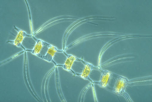
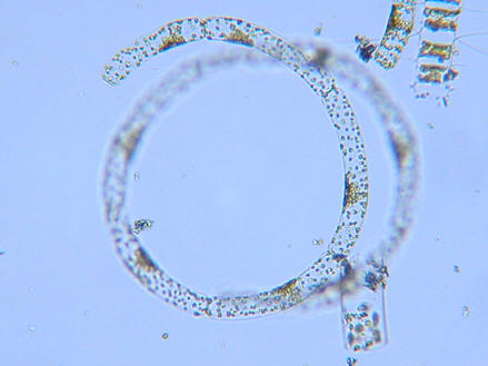
Each station contained a relatively high abundance of Chaetoceros,
Guinardia f., Leptocyndrus d. and Rhizosolemia sp.
Chaetoceros (figure 17) is a colony-forming diatom
found largely in the surface waters receiving high sunlight, which
goes some way to explain its fairly high abundance in each of the
samples taken as it is probably present in the samples nearest the
surface. Guinardia f (figure 18) is found in greatest number
at station 4, with 354 cells compared to 60 at station 3, the second
highest abundance. This could be in accordance with the high
combined input of nutrients from the two estuaries causing high
growth, along with that of other species in this area. Guinardia
s., on the other hand, is found only at station 5, though in
significantly high numbers of 112 per 3ml of sample. This may be due
to this particular species having a late diurnal cycle, occurring
later in the day and in the still water provided here at slack
water, compared to the more turbulent waters found at the other
stations, combined with the outflowing nutrients from the Fal
estuary, most notably a rise in silicate as compared to the morning.
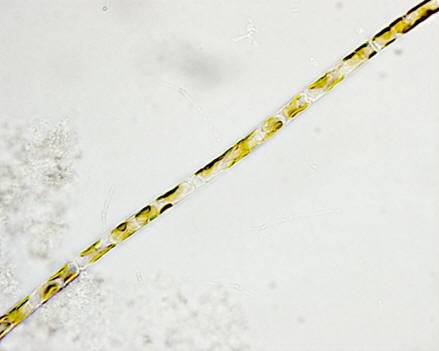
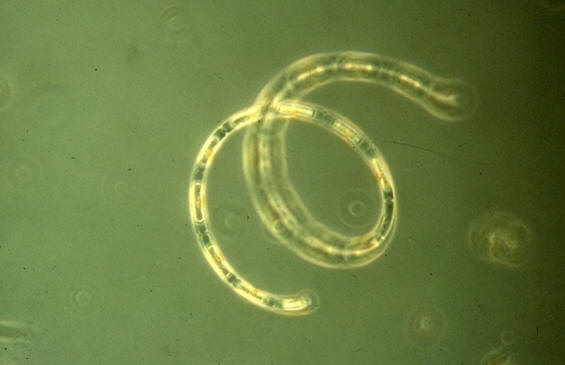
Leptocyndrus d. (figure 19) is the most abundant
phytoplankton found in total, with 570 cells found in total from the
entirety of the samples. Occurring in high numbers at stations 2, 4
and 5, this species appears to thrive in still and stratified waters
rather than more mixed waters. This has resulted in nutrient
boundaries, where nutrients such as silicate and phosphate have
accumulated at depth and may be mixed upwards at a later date to
promote further phytoplankton growth when the stratification breaks
down. Rhizosolemia so. is also found heavily in samples from
stations 2 and 4 though little elsewhere, suggesting again a
preference for deeper, stratified water columns rather than the more
mixed waters of the estuary, given none of these cells were found at
either stations 1 or 5, at the mouth of the estuary.
|
 |
 |
 |
|
Figure 6. Chaetoceros |
Figure 7. Guinardia flaccida |
Figure 8. Leptocylindrus danicus |
 |
 |
 |
|
Figure
9. Abundance of phytoplankton species found at sample
stations |
Figure
10. Percentage composition of phytoplankton species found at
each station |
Figure
11. Other phytoplankton found - Rhizosolenia stoiterfothil |
|
|
 |
|
|
|
Figure
12. Other phytoplankton found - Guinardia strata |
|
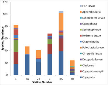
Zooplankton abundance:
As with the phytoplankton, samples
from station 4A held the greatest number of zooplankton, at 105
cells found in a 10ml sample from 35-25m in depth. The abundance of
phytoplankton to feed on at this site is the most probable cause for
the zooplankton numbers though as this sample was taken at the
greatest depth of between 35 and 25m, thus suggesting the
zooplankton follow a diurnal cycle, retiring to depths during the
day to avoid predation then rising towards the surface as night to
feed. This is reinforced by the two samples taken at station 2,
where more zooplankton were found in a 5m stretch between 30 and 25m
depth than were found between 25 and 15m, at 47 and 41 per 10ml
respectively. Such vertical migration is not possible to the same
extent at station 1, at the mouth of the estuary where the water is
not as deep. However, station 1 contains the second highest
abundance of the samples, at 82 per 10ml sample, perhaps indicating
that, due to the rather low abundance of phytoplankton in this
station, zooplankton keep the numbers low by grazing. Upon sampling
higher in the water column at station 4, the total zooplankton found
per sample was only 24 and the phytoplankton population
significantly larger, suggesting the zooplankton had retreated to
lower than the 10m depth of the net.
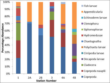
The most frequently found group were
copepods, particularly in the samples taken further offshore, such
as sample 2A, in which 70% of zooplankton found were copepods,
compared to only around 20% for each station 1 and 4B. Copepods are
an incredibly abundant group of zooplankton throughout the world’s
oceans and the Falmouth area is no exception, given the availability
of phytoplankton food supply. Copepod nauplii were also
common, though usually only in stations where copepod numbers were
lower, for example at stations 1, 3 and 4A. Estuaries such as the
Fal and Helford would be used as spawning and nursery grounds for
copepods and other zooplankton, giving a high proportion of larvae
nauplii here and a wide range of groups found at both
stations 1 and 5, both at the mouth of the Fal Estuary. Stations 3
and 4 both also have large populations of copepod nauplii,
though these were both located near the entrance to both estuaries
and thus would be affected by both, including the output of young
copepods and other larvae. Both samples taken at station 2, located
furthest offshore contained no juveniles, only adult individuals, as
once they have reached this far from the estuaries they have fully
grown and are able to feed further out into the ocean. A further
abundant group was the Appendicularia, found in all samples
apart from that at station 3. These tunicates are free-living in the
pelagic zone, thus are found at all depths sampled, though may be
absent at station 3 due to competition from copepods which are far
the most abundant there. As they are in their smallest numbers at
station 1, it can be inferred that they much prefer more stratified
water further offshore from the estuary and are able to thrive
there.
 |
 |
|
Figure
13. Abundance of zooplankton species found at sample
stations |
Figure
14. Percentage composition of zooplankton species found at
each station |
Physical Characteristics
Analyses
|
Figure 15 shows offshore temperature
variability with depth. These stations are very similar because they
are very close to each other (see chart of station locations and
station map). These locations in the estuary mouth are strongly
mixed by both wind and tides, leading to the homogenous temperature
distribution and no discernable water column. These stations are
much shallower than the other stations, so the mixing can go through
the entire water column at this point.
For stations 3,4 and 5, a
thermocline can easily be seen. At station 3, the thermocline is
constant from 13.25 down to 11.5, suggesting mixing between only 2
water masses, the deeper cooler water and the warmer surface waters.
Stations 4 and 5 have more complicated thermoclines with small
plateaus, suggesting more complicated mixing between other water
masses and a possible mixed layer at around 18m. This can be
confirmed by checking our other parameters that we have sampled. It
was hypothesized that wind driven water currents from around Lizard
Point may have been causing this, although with our current samples
we cannot prove this.
|
Figure 15.
Offshore temperature profile, changing with depth
 |
The vertical profiles seen in the figures 16-20 represent the data collected from the CTD at
the five stations, the locations of which can be seen in table 2
and figure 2, the transect map.
Figure 16.
Profile for Station 1 |
Station 1 |
Station 1 shows fairly homogenous conditions through the
water column, demonstrated in particular by the very small
variation in temperature. The irradiance levels follow the
same exponential decrease due to the absorption and
scattering of light by particles in the water column as at
the other stations, but there are much lower values at
station 1; the highest irradiance level at the surface was
~1600PAR, but all the other stations range from ~2000 to
~5500PAR. The salinity has little variation in any of the
profiles, as offshore salinity values have very few outside
influencing factors. The turbidity is recorded on the
transmissometer, and the lower the values, the higher the
turbidity. So at station 1, it can be seen that there is
very high turbidity at the surface and then fluctuates down
through the water column to ~3NTU. The chlorophyll is fairly
stable, but in comparison to the other stations, station
1has higher chlorophyll levels than the others. This could
be due to the higher inputs of nutrients from the inflowing
river (station 1 is closest to the estuary
mouth). Also, it could be due to the high amounts of mixing
caused by tidal activity, as further offshore stratification
affects the transport of nutrients into the euphotic zone.
The other characteristics of these profiles indicate a
well-mixed environment. |
Figure 17.
Profile for Station 2 |
Station 2 |
Station 2 was located at the furthest point offshore on the
transect. The depth profile shows the most stratification
across the stations, as there is a well-defined thermocline
between the ~2m and ~30m. The chlorophyll remains roughly at
about 0.06µg/L through the water column. The lower values
than those of station 1 could be due to the nutrient
limitation in the euphotic zone caused by the stratification
in of the thermocline. The turbidity is higher at the
surface, which is most probably due to wind stress, and then
decreases quickly to just less than 4NTU, and then remains
homogenous. Irradiance decreases exponentially with depth
again, but has higher values at the surface, which could be
indication of more UV rays. Salinity spikes can be seen on
the depth profile, and these are most likely caused by the
time-lag between the CTD temperature and salinity
measurements. |
Figure 18.
Profile for Station 3 |
Station 3 |
Station 3 depth profiles also represent a well-stratified
environment, but the thermocline reaches to almost 40m and
decreases in steps, so there is less stratification and
therefore more mixing, as tidal influences are having more
of an effect closer to the coast. Turbidity is again higher
at the surface because of wind stress, but reaches down to a
slightly greater depth before becoming vertically consistent
at about 20m. Salinity spikes can also be observed on this
profile, as the conductivity is recorded before the
thermistor has had time to warm up at the same rate.
Irradiance levels have a high at the surface of
~4000PAR and decay to roughly 20m before primary
productivity would be no longer possible. This correlates
with increased mixing. Chlorophyll levels are again
consistent at about 0.07 µg/L, but are unusually high at the
surface to about 3m compared to the other stations. This is
most likely linked to the increase in turbidity and decrease
in irradiance. The more particles in the water column, the
less light can attenuate, so with the increase in
chlorophyll it is probable that there is a large patch of
plankton. |
Figure
19. Profile for Station 4 |
Station 4 |
The stratification decreases more again at station 4, as the
tidal mixing increases. The thermocline has become steeper,
and although the turbidity at the surface has decreased
slightly. The main feature of this profile is the
correlation between the turbidity spike and the irradiance
at about 3-4m; the turbidity increases and the irradiance
decreases, so this shows a large patch of noise, caused by
marine animals, anthropogenic features or other objects that
would produce backscatter. There is no increase in
chlorophyll this time however, so it is unlikely to be
linked to plankton.
|
Figure
20. Profile for Station 5 |
Station 5 |
Depth profiles for all the data acquired from the CTD cast
at station 5 are shown. This station is very well mixed and
the depth profiles reflect this fact. From just below the
surface the turbidity is fairly homogeneous all the way to
the seabed. The chlorophyll is also evenly distributed
throughout the water column. Temperature and irradiance also
follow steady curves however the temperature change at depth
is much less than at other stations, proving the homogenised
water column. The salinity shows some large spikes, caused
by the time lag; however the scale of the graph exacerbates
these. The spikes occur over a very short spatial
period and may be the result of incomplete mixing of the
fresh water input in the estuary. |
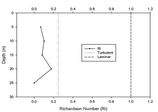
Water Column
Stability
The Richardson number (Ri) is a calculated dimensionless value of
the stability of the water column. It is the ratio of the
stabilising effect of the density gradient to the destabilising
effect of the velocity shear. A Ri number greater than 1 describes
laminar flow and a number less than 0.25 reflects turbulent flow. A
number between these two values is determined by gravitational
shear. The Richardson number is calculated using:

All stations show increasing Ri numbers within the first 5-10
meters, and this indicates that with an initial increase in depth
moving out of the wind and wave driven mixing, the water column
increases in stability. After this depth, the individual
characteristics of each site dominate the stability. Both stations
1 and 5 were taken at Black Rock and the variation seen between
these two stations is a direct result of the tidal cycle. Station 1
was sampled around slack tide resulting in a well mixed turbulent
water mass, whereas station 5 was taken just after low water and has
thus resulted in the appearance of two water masses: a turbulent
freshwater layer extending down to 15 meters and a laminar stable
water mass from 15-20m. The Ri numbers seen at station 2, although
not reaching the laminar threshold, do agree with the CTD data for
this station showing a clear thermocline. At station 3 the majority
of the data points fall below the turbulent threshold indicating
that the water mass is well mixed probably due to the stations
proximity to the coast increase the effects of tidal mixing. The
water mass sampled at station 4 is predominantly stable, and this
may be due to the tidal state, just being after low water, when the
station was sampled.
 |
 |
 |
|
Figure
21. The Ri numbers at station 1 are all below the turbulent
threshold indicating a well mixed water mass. |
Figure 22. The Ri profile of station 2 shows an initial
increase from 5-25 meters however the values do not reach
the laminar threshold. From 25- 35 meters the Ri number
falls and eventually falling below the turbulent threshold
at 35-40 meters. From 40-45 meters the Ri number increases
but again not reaching the laminar threshold. From 45-55
meters the Ri number falls again below the turbulent
threshold.
|
Figure 23. The Ri profile at
station 3 is initially turbulent but does increase from
20-35 meters but not actually reaching the laminar threshold
before falling again to become turbulent.
|
 |
 |
|
|
Figure
24. The Ri profile for station 4 is predominantly laminar
and stable as the majority of the dats points are either
above or around the laminar threshold. However, from
35 metres the Ri falls, eventually falling below the
turbulent threshold.
|
Figure
25. The Ri number for station 5 increase with depth over
5-20 meters showing a change from a turbulent well mixed
water mass in the upper water column to a more stable
laminar flow in deep water. The reduced Ri number at 25
meters could be the result of increased friction from the
bottom of the sea floor.
|
|
ADCP Analyses
|
ADCP data gathered
at the stations offshore indicate the state of the current present
in the water body. The contour plots shown below and their
relevant descriptions highlight this information. Station 1 is
not included as an analysis area itself due to the fact that its
location is the same as that of station 5.
The ADCP figures for the transect between stations 1 and 2 show a
sharp transition from high backscatter and velocity magnitude to
lower backscatter and magnitude. This may be due to a front
occurring at the boundary between the two. The velocity direction
also changes from 50° to 360° with velocity higher on the left of
the track at 0.125m/s compared to 0.250m/s to the right. These
sudden changes may also be due to a deepening of the water column
and change from coastal to offshore processes. The ships track also
shows the change in velocity from transect start to finish.
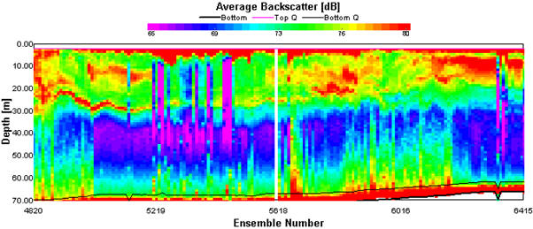
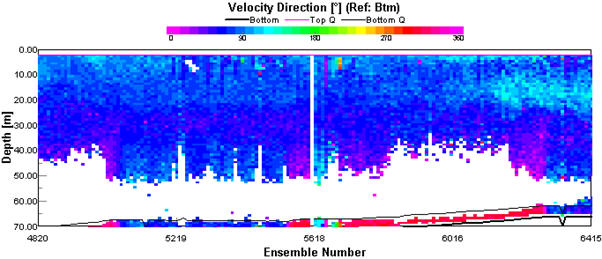
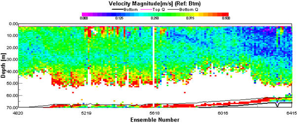
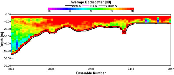
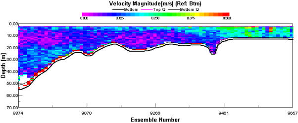
At station 3 the waters were well stratified with a seasonal
thermocline descending to 30m where the waters become well mixed and
uniform in temperature. There is also a band of high backscatter at
30m on the ADCP transect, this reflects a Doppler shift in the
signal received by the ADCP. This may be caused by zooplankton
populations which graze the phytoplankton held above the thermocline
where light is high enough for growth.
|
Figure
26. Average backscatter contour plot, station 2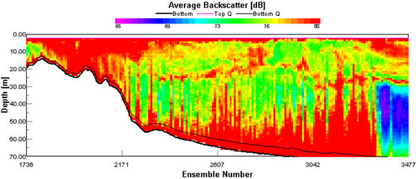
Figure
27. Velocity direction contour plot, station 2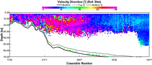
Figure
28. RV ship track, station 2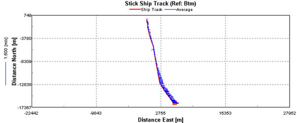
Figure
29. Velocity magnitude contour plot, station 2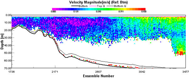
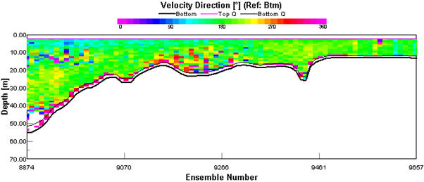
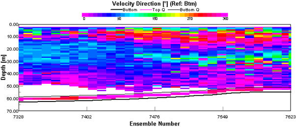
ADCP transects for station 4 show low magnitudes and varying
directions of flow, which increases shear between flows. This data
was taken at slack tide causing lower speeds than the other stations
with a maximum of 0.125 and varying directions due to the change
from flood to ebb. The high backscatter stops at 30m this may be due
to a reduction in down welling irradiance preventing growth of
phytoplankton and therefore zooplankton below the threshold.
Figure
34. Average backscatter contour plot, station 4
Figure
35. Velocity magnitude contour plot, station 4
Figure
38. Velocity direction contour plot, station 5
 |
|
Figure
30. Average backscatter contour plot, station 3
Figure
31. Velocity direction contour plot, station 3
Figure
32. Velocity magnitude contour plot, station 3
Figure
33. Velocity direction contour plot, station 4
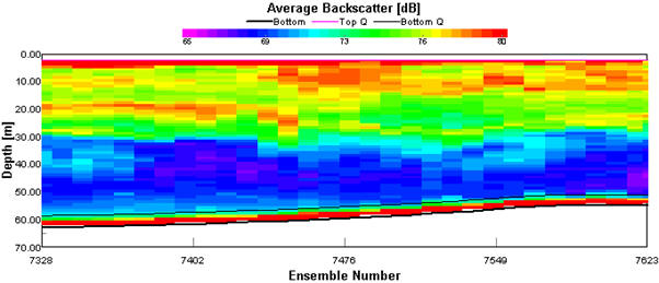
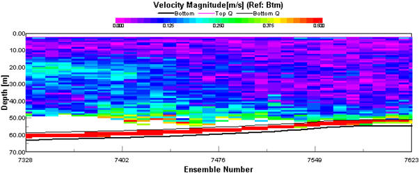
Station 5 represents a well mixed water column with a relatively
uniform profile for direction and magnitude with a maximum of 0.2m/s
at 180°. Some vertical shear flow is evident in the velocity
direction plot. The backscatter is higher than at other stations as
available nutrients from river inputs are higher than at the
stratified stations, thus sustaining higher populations of
phytoplankton and thus zooplankton throughout the water column.
Figure
36. Average backscatter contour plot, station 5
Figure
37. Velocity magnitude contour plot, station 5
 |
Irradiance
|
|
LUP 1% Depth (m) |
|
Station 1 |
* |
|
Station 2 |
44.92 |
|
Station 3 |
38.76 |
|
Station 4 |
47.25 |
|
Station 5 |
* |
Table 5. LUP 1% light depths for stations 1-5. Stations bearing '*'
indicate water too shallow to calculate a 1% light attenuation
depth. |
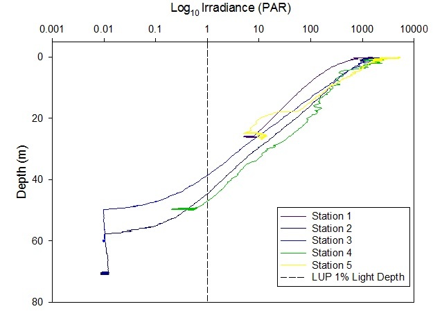
Figure 39 demonstrates an
exponential trend in irradiance decrease with depth at each station.
At station 4, the irradiance seems to still be high at lower depths
than at other stations (47.25m), whereas both stations 1 and 5 (both
taken at Black Rock) do not reach their LUP 1% light depths as there
was not a deep enough water column.
By observing the plots
generated from the ADCP data, it is possible to see that there is
more backscatter in the water column in stations 2 and 3 than
station 4; this allows more penetration of light and a deeper LUP 1% irradiance depth. A higher stratification index at station 4
implies minimal mixing and more stability in the water column.
|
Figure 39. Log of irradiance down the water column for stations 1-5 with
their LUP 1% light depths.
 |
Conclusion
The offshore investigation has shown that the water extending from black
rock away from the Fal estuary becomes progressively more stratified
with distance offshore. This is due to the deepening of the water column
which reduces the mixing effect of the tide on offshore waters. The
degree of stratification was less than would be expected in July, as
wind stress and subsequent mixing has been higher than an average year.
Station 2 showed a seasonal thermocline above which phytoplankton growth
was contained. The silicate and phosphate data was low at station 2 as
the thermocline prevents upward nutrient mixing from the layers below
and phytoplankton populations utilise any available nutrients for
growth. The ADCP transect between station 1 and station 2 showed
possible presence of a frontal system with a boundary formed between
areas of stratified and mixed waters, which also marks the transition
from coastal to offshore waters where tidal influence is reduced.
Station 2, 3 and 4 therefore fall on the stratified side of the boundary
with solar heating causing seasonal thermoclines to form in the upper
30m, whereas stations 1 and 5 are located on the well mixed side where
tidal velocities and shallow depths break down any stratification from
heating and therefore conditions remain relatively homogenous throughout
the water column.
Station 1 and 5 show decreasing nutrient concentrations with depth as
mixing and irradiance allow for growth throughout the whole water
column, whereas nutrient concentrations from 2, 3, 4 increase with depth
as nutrients are able to replenish below the thermocline as growth is
limited by light. This is also reflected in the dissolved oxygen
concentrations for each station.
For a future investigation more stations would be needed to provide
evidence of a definite frontal system between stations 4 and 5 before
firm conclusions could be made.
|
|


 |
Geophysics Mapping - SV Xplorer 02/07/2012 |
|
Introduction
Tables 6 and 7.
Meteorological data and tides for geophysical work
|
Date |
02/07/2012 |
|
General Weather |
Overcast with rain |
|
Visibility |
Very poor |
|
Sea State |
Calm |
|
Cloud Cover |
8/8 |
|
02/07/2011 |
Tide Times GMT |
Tidal Height (m) |
|
High Water |
0427 |
4.80 |
|
Low Water |
1110 |
0.80 |
|
High Water |
1655 |
5.00 |
|
Low Water |
2342 |
0.70 |
|
The aim of this investigation was to
gain an understanding of the habitats on the river bed using side-scan
sonar followed by ground truthing using an underwater video camera.
The investigation was carried out on
the hydrographical survey vessel, Xplorer. A route was planned along the
River Fal based upon weather a tidal conditions, which can be seen below
in figure 36.
An understanding of the river bed
substrates and habitats will enable us to recognise ways in which
impacts of human activity can be managed. It will also increase our
understanding of possible impacts of climate change.
The Fal
Estuary was selected for habitat mapping as it is a Special Area of
Conservation (SAC) and is therefore recognised as the location of some
habitat types and species considered to be most in need of conservation
(www.defra.gov.uk).
Maerl beds are an important habitat within this area of conservation.
Table 8.
Conditions during the geophysical investigations
|
Date |
02/07/12 |
|
High tide |
15.27 UTC |
|
Low tide |
10.10 UTC |
|
Vessel |
SV Xplorer |
|
Time |
08.45 -
11.08 (UTC) |
|
Temperature |
14 - 16°C |
|
Weather |
Rain |
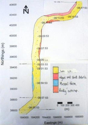
The majority of the substrate in the
river is soft silt, which can easily be seen on the habitat map. The
very centre of the channel is free of features, due to the faster flow
in the deepest areas. At the first video site at roughly 40600N 185000E,
the sidescan showed homogenous silt on the bed however, there was a
large amount of leaf litter and shells covering the sea bed. These were
not picked up on the side scan and provided more habitats than were
expected after initial evaluation of the sidescan. Between 40550N
184850E and 40400N 184400E there is an abundance of algae and shell
debris. This corresponds with the slower flow rates on the inside of the
meander, which allows the algae a more stable area to grow without being
washed away. Shells were very difficult to identify from video footage
and most of the algae seen was Rhodophycae of differing genera.
One of the only other distinct
features on the sidescan that was transferred onto the habitat map was a
rocky outcrop all along the right hand bank running for almost a
kilometre. Although it had little effect on the sidescan, the mussel
farm between 39400N 184150E and 38900N 184150E may have had quite an
effect on the seabed. The two videos, one upstream and one downstream of
the mussel farm: These two areas were a stark contrast, however it was
suspected that there were other factors than just the mussel farm at the
very desolate video station above the farm. This may have been partly
due to the effects of the pontoon and also unusually poor light
attenuation in the area. The only other interesting areas on the side
were the large cargo ships that were moored on the river being
superimposed on to the sidescan track. These were not included on the
habitat map as they were not actually on the seafloor.
The following thumbnail
is to further detailing of our investigations and habitat map.
Click it to enlarge!
 |
Figure
40. Geophysical
investigations route; including habitat mapping and video
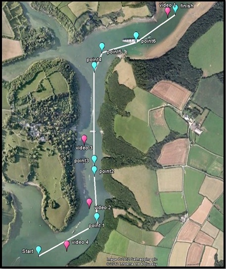
Figure 41. Overview of
habitat map generated
|
|
|


 |
Estuarine Work -
Pontoon 26/06/2012, Fal Estuary 04/07/2012
|
Date |
04/07/2012 |
|
General Weather |
Overcast with rain |
|
Visibility |
Very poor |
|
Sea State |
Choppy |
|
Cloud Cover |
8/8 |
|
|
|
Tables 9 and 10. Meterological data and tide data for estuarine work
|
04/07/2011 |
Tide Times GMT |
Tidal Height (m) |
|
Low Water |
0047 |
0.70 |
|
High Water |
0651 |
5.30 |
|
Low Water |
1311 |
0.70 |
|
High Water |
1910 |
5.60 |
|
A scientific boat trip was undertaken throughout the Fal estuary to
determine the type of estuary and also the key chemical, physical and
biological behaviour within it. The estuary is where fresh and sea water
mix, leading to interesting chemical, physical and biological
conditions. Similar factors will be measured to the offshore boat
practical however very different results are expected. The data compiled
on the boat coupled with the pontoon data will provide a comprehensive
overview of the processes at work in the estuary.
In recent years, the Fal has had numerous problems with heavy metal
pollution (Bryan & Gibbs, 1983) from mining run off; which have been
known to have an effect on the trophic assemblages within it (Warwick,
2001). Mining operations at Wheal Jane and other mines have since ended
but metals may still be leaching into the estuary and causing problems.
Some of the pollution may still be present and the residence time of
water in the estuary shall be calculated to see how much of an effect
the past problems may still be affecting the sediments and associate
assemblages (Somerfield et al, 1994). Brown seaweeds may be an indicator
of continuing problems as they have been known to be indicators of trace
metals (Luoma et al., 1982 & Bryan, 1983)
For this work, the Bill Conway was used in order to take lagrangian
measurements, simillar to those taken on the pontoon
at stations throughout the estuary. ADCP transects of the river at 5
different locations gave a profile of the speed and direction of flow
beneath the boat. Secchi disk measurements allowed the depth of the
euphotic zone to be estimated and the light attenuation to be inferred
from this. CTD profiles and niskin bottles at 3 different locations
allowed a complete, salinity, temperature and chemical profiles with
depth.
From the water samples collected, sub samples were taken in order to
calculate the chemical values of dissolved oxygen concentration,
nitrate, phosphate and dissolved silicon; back in the lab. Data was
taken throughout the day by two groups from both the top and bottom of
the estuaries to give a full profile from the river to the sea. Samples
in the morning were taken from the top of the estuary down, into the
onrushing tide, so that the same pocket of water wasn’t follow, with the
opposite being done in the afternoon for the same reason. |
Figure 42. Plot of transects taken within
the estuary
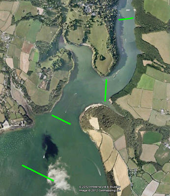 |
Figure 43. Track plot of RV Bill Conway
throughout the estuary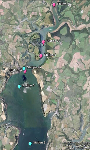 |
Pontoon
Eulerian measurements were taken at King Harry pontoon
(50°12.970N, 005°01.659W) in conjunction with group 7 who took
measurements in the morning, with group 6 (us) taking over in the
afternoon. Salinity, temperature, pH, dissolved oxygen and chlorophyll
data were recorded using a
YSI probe at 1m depth intervals. A light
meter and ADCP were also used to measure down welling irradiance and
vertical current profiles. Each profile was taken every 15 minutes
throughout the day to establish a full time series of vertical changes
in the properties over a complete tidal cycle.
 |
 |
 |
 |
|
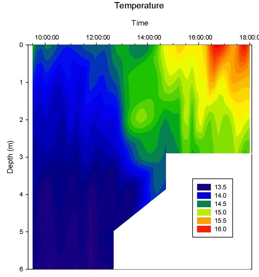
Figure 44.
Temperature contour plot, pontoon |
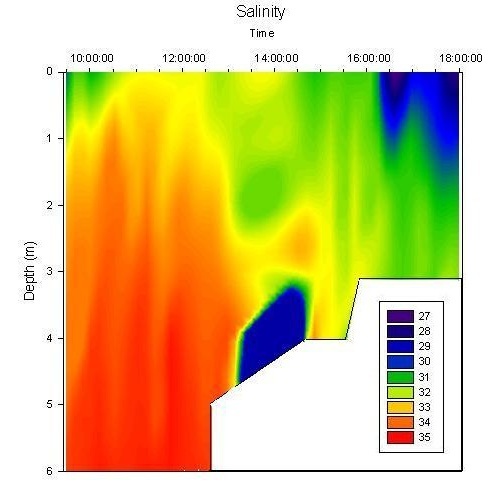
Figure 45.
Salinity contour plot, pontoon |
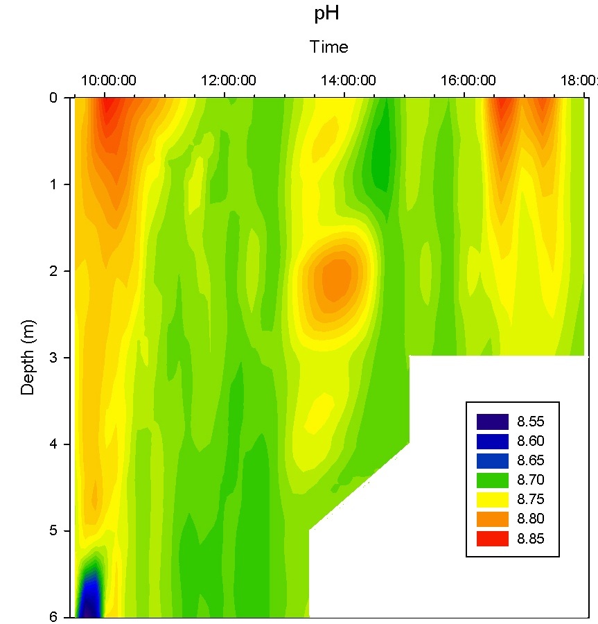
Figure 46. pH
contour plot, pontoon |
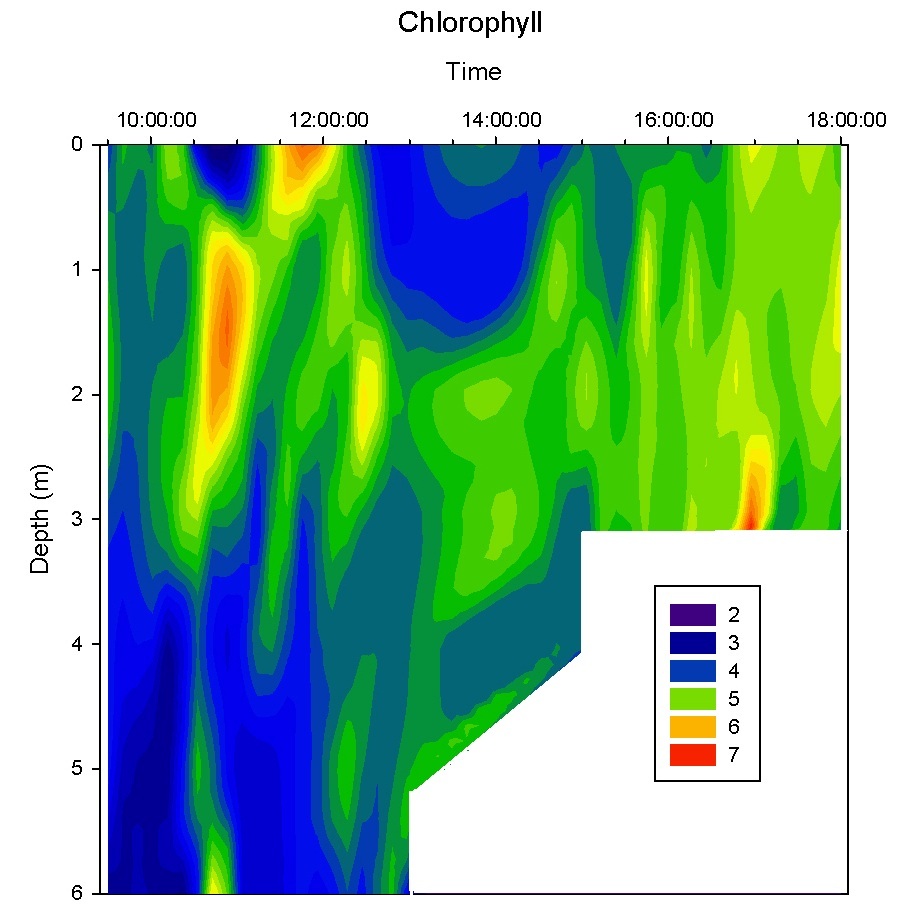
Figure 47.
Chlorophyll contour plot, pontoon |
Table 11. Detailing
relating to figures 44-47 above
|
Temperature |
The temperature shows a small variability throughout the day,
figure 44. In the morning starting at around 0930, the incoming
tidal flood produces the large amount of cold water at all
depths. After high tide, the warmer river can be seen pushing in
and dominating at around 1630 onwards. The gradient in between
these two areas is where the mixing of the two waters is
occurring at around slack tide. |
|
Salinity |
The contour plot (figure
45) for salinity shows a vertical
transect throughout the day. Earlier in the day between 1000 and
1200, the higher salinity shows the tidal flood up the river.
This continues up until high tide, after which, the salinity
decreases as the river begins to dominate the flow. The blue low
salinity section is caused by extrapolation due to missing data
as the morning and afternoon groups changed over. In the
afternoon, starting at around 1630, the lower salinity river
water can be shown flooding down the river as low tide
approaches. |
|
pH |
Hourly small variations are seen throughout the day at the
pontoon. This may correspond with changes in solar radiation
throughout the day. The activity of the phytoplankton and other
photosynthetic organisms will lead to the slight change in pH
seen, figure 46. |
|
Chlorophyll |
The contour plot, figure 47, shows maximal chlorophyll values at
around 1030, this is a slight lag from the first light of the
day. There is a then a dip in this throughout the water column
with the maximal values still being around 2m. The rise and fall
of the chlorophyll follows the very patchy solar radiation that
occurred on that day, with a peak coming in the evening with
high values throughout the water column; as it is relatively
homogenous at slack tide at around 1700. |
Physical Characteristics
Analyses:
CTD Data
Note:
Stations are named 4 and 4a because the two groups sampling the
estuary measured stations 1-4 then 4-6, where the last and first
stations respectively were in the same position.
Hence 4
and 4a for the split group sampling.
Figure 48.
Station 1 estuarine depth profiles |
Station 1 |
The depth profiles for station 1 were taken at the furthest
point up river of the transect. The temperature values decrease
from about 14.9⁰C
at the surface to about 14.5⁰C
at 6m, a few centimetres from the bottom of the riverbed. The
salinity follows the opposite pattern, as the lowest value is at
the surface and increases down through the profile, with the
highest value at ~6m depth. There is little variation in the
turbidity; it has slight fluctuations through the water column
around 3.8NTU, but does show more of a slight increase where
there is a sharp spike in salinity, at about 4m. The main
feature of the fluorometer data is the spike of chlorophyll, as
it increases suddenly at ~3.8m from ~0.3µg/L to 0.7µg/L, and
then decreases back at ~4m. |
Figure 49.
Station 2 estuarine depth profiles |
Station 2 |
There is an inverse relationship between salinity and
temperature at Station 2. There appears to be a slight
thermocline in conjunction with a possible halocline at around 2
to 3 meters, though the overall changes are relatively small
(0.7°C). The turbidity changes throughout the water column are
minimal, with no apparent, significant change with depth. The
chlorophyll readings show peaks at around 4, 8 and 11 meters,
this suggests potential phytoplankton activity at these depths
and can be related to irradiance levels. |
Figure 50.
Station 3 estuarine depth profiles |
Station 3 |
Station 3 profiles were taken further towards the end of the Fal
River, closer to the open estuary. The temperature values
decrease down the water column over a range of 0.4°C, in a
similar pattern to all the other stations. Salinity also
imitates the previous two stations and increases down the
profile, but has a slightly steeper slope so does not become
more saline until ~3m. The temperature and salinity profiles
both roughly show small spikes and curves at the same depth;
they are mirror of the other. The chlorophyll and turbidity both
have small fluctuations through the water column but do not have
very large changes in value, although chlorophyll does have a
relatively large peak at the surface (of ~0.4µg/L). |
Figure 51.
Station 4 estuarine depth profiles |
Station 4 |
Station 4 was taken at the mouth of the
river and at the top of the open estuary. The temperature and salinity again
exhibit an inverse relationship, and display the same small
fluctuations at the same depths along the profiles. A slight
thermocline and halocline can be seen at ~8m, although both are
relatively steep. Turbidity decreases with depth, by ~1NTU.
Small spikes down the chlorophyll can be seen, and one
particularly large increase is present at ~10-11m; the values
change from 0.2 to >0.5µg/L. There is also a well-defined,
albeit smaller, spike at 4m. |
Figure 52.
Station 4a estuarine depth profiles |
Station 4a |
Station 4a is at the same location as station
4, but was repeated later in the day so as to gain a range of
data over the day of the same point. The temperature at the
surface is slightly greater than at station 3 (15°C), and starts
to decrease down the water column, before increasing in a small
bulge around 4m, and then returning to the familiar decreasing
pattern and ending at 13°C at the seabed. The salinity increases
fairly steadily from ~30.5 at the surface to ~34.5 at the bed,
with the occasional small fluctuations. The turbidity decreases
slightly down the profile, except for a sudden increase at ~5m,
correlating with a chlorophyll spike at the same depth. The rest
of the chlorophyll profile is fairly uniform, with a few smaller
spikes towards the bottom. |
|
Figure 53.
Station 5 estuarine depth profiles |
Station 5 |
Station 5 shows slight amount stratification, with a steep
thermocline and halocline at ~4m. The salinity increases down
the water column by about 3.5, and the temperature decreases by
1.6°C. There is a small increase in turbidity between the
surface and 2m, which corresponds with an increase in
chlorophyll. Both then decrease again between 2m and 4m. Smaller
chlorophyll spikes further down the profile also correlate with
changes in turbidity. For example between 6m and 8m, when
chlorophyll values decrease from ~0.25 to ~0.15, and turbidity
shows a small corresponding decrease. |
Figure 54.
Station 6 estuarine depth profiles |
Station 6 |
Station 6 was recorded as the final location at the end of the
transect closest to the open sea. The temperature and salinity
profiles again are the inverse of each other, and demonstrate
two slight thermoclines and haloclines at ~4m and then again at
~17m. This may be the result of mixing of three water masses
rather than just two, which would construct only one thermocline.
The water is much more saline at the surface than at the other
stations, but there is not such a great increase down the
profile. The turbidity also decreases in similar stages as the
salinity and thermocline patterns, with larger decreases at 4m
and 7m. The chlorophyll shows little variation, although there
are slight increases in the size of the spikes between 10 and
15m. |
The temperature in the estuary is coldest in morning and warmed
throughout the day, whilst also becoming colder with depth. From both
the pontoon and CTD measurements, similar results were gathered, though
the data gathered on the pontoon was 0.2⁰C lower than those of the CTD.
Although small, this difference shows a slight warming in the 8 days
between the measurements being recorded.
There are incredibly significant differences in chlorophyll measurements
from the pontoon YSI probe and boat CTD, leading to discrepancies on the
graphs for this data. The CTD measurements were recorded to be between
approximately 0.22 and 0.26µg/L whereas at a similar time from the
pontoon measurements fell between 3 and 5µg/L, largely due to issues in
calibration of the instruments and also with Sigmaplot, the graph
software used to create the contour plot of pontoon data extrapolating
values to fill in gaps, which may not have been accurate.
Salinity increases with depth at this station with measurements from
both the CTD and probe off the pontoon, though, like salinity, there is
a slight difference between the data, whereby the CTD recorded results
approximately 2 salinity units below those of the probe off the pontoon,
throughout the depth of the estuary. This may be due to calibration
issues, or more likely due to the significant difference in salinity
measurements because of the change in tidal state at this time on the
two different days, indicating whether the river is at that moment
marine or riverine dominated.
Discussion
The Fal estuary is a well-mixed estuary and is tidally dominated, with a
semi-diurnal tidal cycle. High tide on 04/07/12 was at 05:19UTC and low
water was at 12:04UTC, so stations 1 to 4 were taken as the tide was
going out and stations 4a to 6 as the tide was coming in.
As temperature and salinity have an inverse relationship at the majority
of the stations, it is appropriate to say that the tide has the greatest
influence over both, and dictates the extent of mixing between the
overlying freshwater from the riverine inputs, and the underlying saline
water. This is why at stations 1 and 3 located towards the top of the
river, salinity is lower at the surface and greater at the bed, and the
temperature is greater at the surface and decreases down the profile,
yet there are no identifiable thermoclines and haloclines due to the
extent of mixing during the ebb tide.
Even though station 2 was located in between those two stations, the
water body is much deeper, meaning that the same amount of mixing would
not be possible. The salinity increases from the start to the end of the
transect, as stations closer to the mouth of the estuary will evidently
be more influenced by saline water than fresh river water. After station
3, the thermoclines and haloclines begin to become more defined, due to
the increased depth of the water column and other influencing factors.
Station 4 was taken at low water, so less tidal mixing would occur and
so slight stratification could develop. Station 4a was taken as the tide
was coming in, and less of a thermocline and halocline are present,
which further proves the extent of the tidal mixing. Station 6 was taken
at 13:58UTC, so the tide had started to come in, demonstrated on the
graph as a breakdown in stratification developing during slack tide.
The general pattern between chlorophyll and turbidity is that with an
increase in chlorophyll, there is also an increase in turbidity. This is
because thicker layers of phytoplankton are present, meaning that there
are more particles in the water column, increasing the turbidity values;
an example of this is at 5m at station 4a. The chlorophyll spikes
correspond with the level of stratification and the depth of the
euphotic zone. From the riverine end to the marine end of the transect,
the euphotic zone becomes deeper and so primary production increases. It
is common in estuaries for the phytoplankton production to mirror the
distribution of suspended sediments (Cloern, 1987). The distribution and
availability of nutrients is also a factor in phytoplankton growth and
therefore also the chlorophyll production. Stratification affects this,
and so the more well stratified the station, the more likely it is for
there to be increased chlorophyll at the thermocline, although the
extent of tidal mixing in this estuary will usually counteract this.
Richardson Number
|
Figure 55. The Richardson numbers (Ri) for the four stations sampled by
Group 6, For station 1, the Ri
numbers are all within the boundary to dictate turbulent flow. The Ri
numbers at station 2 are all below the turbulent threshold of 0.25 down
to 7m and from this point, the numbers increase but not reaching the
laminar threshold, except at 12m. The Ri numbers for station 3 all
dictate turbulence down to 8m, then the values increase over the 1.0
threshold for a laminar flow. Station 4 shows a similar profile to that
of station 3, where the Ri numbers are below the turbulent threshold
down to 5m, then between 6-7m the Ri numbers are above the laminar
threshold, and below 8m the values vary around the laminar threshold.
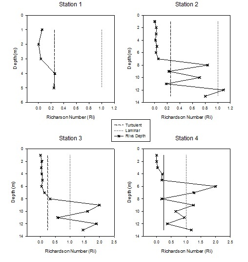 |
Figure 56. The station average Richardson Number (Ri) for all the
stations sampled across all stations showing laminar flow at each
location.
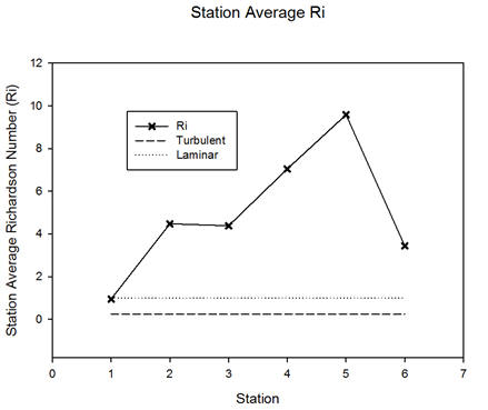
When comparing the Ri
numbers seen in figure 55 and those seen in figure 56, a discrepancy is
seen; if using the results in figure 55, Ri numbers are generated by
averaging the entire water column, where all the stations can be
classified as having a laminar flow and the estuary being stratified.
However, when examining each station in more detail and calculating the
Ri numbers with decreasing depth, a more complex profile is generated.
Station 1 is positioned towards the source of the estuary just above the
joining of the Truro and the Fal rivers, and a well mixed water column
is seen rather than the laminar flow with stratified water column
predicted when using figure 55, which integrated all the points with
depth. The profile for station 2 is also more complex than the whole
water column average as the upper water column generates Ri numbers
showing this section to be turbulent and as a result well mixed.
However, the lower section of the water column below 7m shows Ri numbers
increasing toward the laminar threshold, indicating the intrusion of a
more stable water mass moving up the river.
This
profile is also seen for stations 3 and 4, but at both stations the Ri
numbers for the more stable water mass extend above the laminar
threshold, and occur below 8m and 6m for stations 3 and 4 respectively.
It can be useful to generate an image of how the Ri number changes along
the estuary averaging across the entire water column as in figure 56,
but the complexity of the water column is missed and can only be truly
seen when a more detailed survey of the Ri numbers is generated as in
55.
|
|
Chemical Analyses:
Phosphate
The
phosphate mixing diagram shows that there is addition of phosphate into
the estuary waters above that predicted by the theoretical dilution
line. This addition may be due to sewage outfalls into the estuary from
Tresillian river (50°16.540 N, 5°0.460 W) and Truro river (50°14.900 N,
5°02.600 W) which join at Malpas (50°14.3981N, 5°01.2382W). This
anthropogenic input of phosphate may help increase concentrations to
above natural levels. Sewage output in this location has been monitored
by the Marine Biological Association with26-62% of phosphate inputs to
the estuary due to sewage (Langston et al., 2003).Phosphate is
acting non-conservatively, meaning a process other than mixing is
affecting its concentration with increasing salinity as you move from
riverine end to estuary mouth.
Chlorophyll
The
chlorophyll concentrations from each station are shown on the graph
below. For the first three stations only 2 samples were taken, the
fourth site was a high resolution site and 5 samples were taken
throughout all depths, giving a more detailed picture of the water
column.
Stations 1
and 3 showed slight decreases at depth, due to the decreasing light
penetration, causing lower chlorophyll concentrations. Station 2 shows
an increase at depth, which is not expected. This may have been due to
the station being close to the pontoon, where a lot of boats come
through. Due to the boats, increased mixing is induced in the water
column, leading to the down welling of chlorophyll. The higher
resolution of station 4 shows a decrease then an increase at depth. The
slight increase may be due to increased tidal mixing as the tide floods
into the estuary. The varied results below this may be due to increased
tidal mixing as high tide is reached around station 4.
Nitrate
The
riverine end member has a very high nitrate concentration of
26.5µm.
At mid salinities, there is a large removal of the nitrate,
showing that it is non-conservative. This may suggest a
phytoplankton bloom occurring in the mid estuary. This bloom may
be due to the degradation of leaf matter releasing extra nitrate
into the water column.
Oxygen
All the stations sampled yielded O2 saturations that are
under-saturated. The highest saturations are seen at stations 1-4. These
were the stations furthest up the estuary, with station 1 being above
the section of the estuary where the Fal joins the Truro, and all
subsequent stations being progressively seaward. However, stations 4 and
4a (4 and 5 on figure 60) were both taken at Turnaware Bar. The
under-saturation seen at all stations is an indication that O2
consumption is greater than O2 production.
At stations 1 and 3, the O2 saturation increases with depth
and reaches 100% at the deepest point sampled at each station. The
stations furthest towards the mouth of the estuary, 5 and 6 (6 and 7 on
figure 60), show an O2 saturation maximum at depth, and this
may be the result of a seawater intrusion entering the estuary below the
freshwater exiting the estuary.
Silicon
The graph displays a Theoretical
Dilution Line of silicate down the estuary (starting from the
Fal River) and demonstrates a non-conservative behaviour of the
nutrient. The plot suggests that there is a removal of silicate
from the estuary at the more saline waters, where diatomic
activity is highest.
|
Figure 57. Estuarine mixing diagram with enlarged section, phosphate
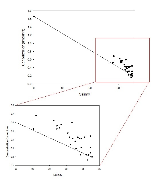
Figure 58. Chlorophyll
concentrations observed at all estuarine stations
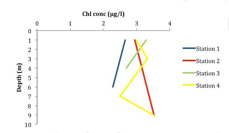
Figure 59. Nitrate
mixing diagram for estuarine water samples
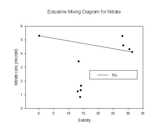
Figure 60. The O2 saturation for all six stations sampled by
groups 6 and 2, stations 1-4 and 5-7 respectively. Stations 4 and 5,
depicted by a hashed line, are at Turnaware Bar at different times
during the tidal cycle. All stations are under saturated.
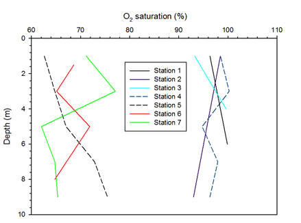
Figure 61.
Dissolved silicon mixing diagram
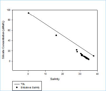 |
Biological
Characteristics Analyses
Phytoplankton Abundance
The afternoon samples taken at
station 4a and 6 contained the highest concentration of phytoplankton,
at 430 and 380 per ml compared to a mere 29 per ml at station 4 in the
morning. Earlier in the morning, in the riverine sample at station 1, no
phytoplankton were found at all. This is testament to the effect of the
tide, which, in the morning, was on its way out, flushing the
phytoplankton out along the estuary whereas in the afternoon was its way
back in, bringing with it a large concentration of phytoplankton.
Furthermore, the afternoon irradiance was much greater due to better
weather conditions and less cloud cover, which would promote
phytoplankton vertical migration towards the surface. As phytoplankton
trawls were carried out only at 1-1.5m depth, this vertical migration to
take advantage of the sunlight near the surface makes a measurable
difference to concentration of cells.
Furthermore, there was a greater
species diversity found at station 6, with a wide range of cells in this
sample, taken from near the estuary mouth where the water is much that
of the ocean, suggesting a preference for most of the organisms to be in
fully saline water rather than the more brackish water of the estuary.
However, station 4 and 4a at the top of the estuary are far less
diverse, and dominated mostly by Rhizosolenia spp. and
Leptocylindrus d. in the morning and Coscinodiscus spp. and
Alexandrium spp. in the afternoon, suggesting that these groups
much prefer the slightly fresher water provided here and have carved
themselves a niche in this area, allowing them to thrive in greater
numbers, particularly in the case of station 4a.
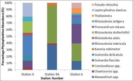 |
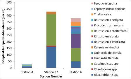 |
|
Figure 62.
Percentage abundance of phytoplankton species in the estuary |
Figure 63.
Species abundance of phytoplankton in the estuary |
Zooplankton Abundance
Morning samples were taken both at
station 1, where the Fal River meets the Truro and station 4; the top of
the estuary, as shown by the map (figure 44). Samples by the afternoon
group were performed at a similar location by the top; station 4a and at
the bottom of the estuary near the mouth; station 6.
At 102, 94 and 84 individuals per
10ml of sample, the three stations on the river and top of the estuary
contain a similar concentration of planktonic organisms. In these cases,
copepods and their nauplii account for approximately 70% of the
individuals found (figure 64), though the nauplii account for a
greater proportion at stations 4 and 4a at the top of the estuary. Being
nearer the sea, they are composed of far more saline water, and thus
contains a greater number of certain organisms found rarely in lower
salinity water up the river, such as Hydromedusae, Ctenophora and
Siphonophorae. These are far more common in saline and brackish
water than they are in fresher water and are also found in considerable
numbers at station 6, with Hydromedusae being the most
significant group behind copepods and their nauplii, 38 specimens
found in the sample, more than twice that found at station 4a. Coupled
with the much greater abundance of zooplankton at station 6, this
suggests a far greater tolerance by zooplankton to seawater, given the
salinity of 35.5 at this station compared to the fresher water found
further up the estuary and river. An interesting feature of station 6,
and to a lesser extent station 4a was the much greater abundance of
copepod nauplii compared to adult copepods; almost four times the
amount at station 6. This may be explained by the copepod breeding
season usually occurring from December to March annually (Conover,
1967), meaning that many nauplii will be almost fully grown, and
some copepods will have just reached maturity so are being flushed out
towards the ocean from their estuarine nursing grounds, especially given
how the salinity varies relatively little along a large portion of the
estuary. The relatively small quantities of Polychaeta, Gastropoda and Decapoda larvae, amongst others, present in samples taken
at all stations suggests that these have most likely settled or fully
grown and as such are rarely found as planktonic larvae.
|
 |
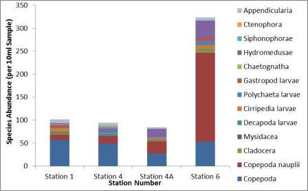 |
|
Figure 64.
Percentage abundance of zooplankton species in the estuary |
Figure 65.
Species abundance of zooplankton in the estuary |
Irradience
Table 12. Calculated secchi disk values
|
Station
number |
Depth |
Secchi
disk depth (m) |
Depth of
euphotic zone- 1% light level (m) |
Attenuation coefficient (k) |
|
1 |
6 |
2.8 |
8.4 |
0.51 |
|
2 |
14 |
3.4 |
10.2 |
0.42 |
|
3 |
14 |
3.6 |
10.9 |
0.40 |
|
4 |
14 |
4.0 |
11.9 |
0.36 |
|
5 |
8 |
2.3 |
6.9 |
0.62 |
|
6 |
20 |
3.8 |
11.4 |
0.38 |
The
secchi disk data show that the depth at which the disk can no longer be
seen increases as you move from riverine to marine end of the estuary,
with the exception of station 5. Increasing channel depth reduces the
effect of flow shear on the sea bed, lowering the effect of suspended
particulate material causing absorption of light in the water column.
The
attenuation coefficient, k, measures how quickly light is absorbed in
the water column; the highest value is seen at station 5 which
corresponds also to a reduction in secchi disk depth. The channel depth
is lower at station 4 than station 5, whilst the tidal state was
flooding into the estuary. High tidal flow and shallow depth would
increase attenuation as sea floor sediments are suspended. This would
cause a high k value as light is absorbed by suspended matter reducing
the secchi disk depth.
Figure 66. Graph to show the depths at which the secchi disk could no
longer be seen when lowered into estuarine water
|
|
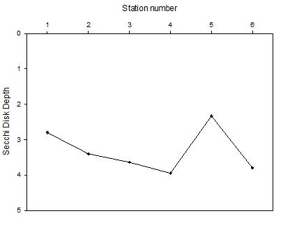 |
|
Residence Time
Tres=[1-(Smean/Ssea)*Vtotal)/R
Tres is
residence time of the estuary
Smean
is mean salinity of the estuary
Ssea is
the salinity at the furthest point of the estuary, closest to the sea
Vtotal
is the total volume of the estuary
R is the river
flux into the estuary
The residence
time is the amount of time a substance remains in a system, so in this
case the length of time a molecule of water stays in the Fal estuary
after entering from a river and before entering the ocean. It is a vital
component when calculating the time a pollutant or contaminant will
remain in the estuary after accidental excessive anthropogenic inputs.
An estuary with an efficient residence time is often more healthy in
terms of water quality and marine life than a poorly flushed estuary. In
order to calculate the residence time, it is assumed that the estuary is
in a steady state; there are no changes in volume, temperature etc.
In order to obtain
the residence time for the Fal estuary, the salinity values along the
length of the estuary were measured via a CTD on board RV Bill Conway
during the estuarine investigation (see estuary data for exact
locations). Seven cross sections of the estuary were also recorded by
the ADCP as the stations moved from river end to marine end. From this
it was possible to access the areas of each of these cross sections by
using the ADCP data in WinriverII, and the distance between the cross
section transects were measured in order to then work out the total
volume of the estuary – 26789460.7m3 = 2.7*107m3.
The mean salinity was calculated from the CTD values (30.6725), and the
final salinity reading that was taken at station 6 was used as the sea
salinity (35.1).
The data for the
river fluxes into the Fal estuary were acquired from the Centre for
Ecology and Hydrology website. The three rivers that feed into the
estuary are the Kennal, Kenwyn and Fal, and their average annual fluxes
have been recorded from 1968-2010 for the Kennal and Kenwyn, and from
1978-2010 for the Fal. These gave results of 0.51m3, 0.378m3
and 2.028m3, respectively, which were then added together to
give a total riverine flux of 2.916m3.
All of these
values were then entered into the equation, and finally divided by 86400
(number of seconds in a day):
Tres=([1-(30.6725/35.1)*26789460.7)/2.916)/86400
=(3379211.87/2.916)/86400
=1158851.813/86400
=13.41days
This is however an
estimate of the residence time rather than en exact calculation, partly
due to the necessary assumptions, but also because the final ADCP
transect did not fully record all the data as the depth was greater than
20m and so the sonar beam could not reach the bottom. The area of this
cross section was then approximated from the existing data of the
shallow edges of the estuary on WinriverII. |
Conclusion
From our investigation of the
Fal estuary it can be concluded that the tidal mixing is the dominant
force within the estuary, influencing biological, chemical and physical
processes, and producing a well mixed estuary.
The data
collected from the time series on the King Harry Ferry pontoon and
during the river cruise on the R.V Bill Conway show the complex nature
of the estuary and the extent of the tidal mixing. The extreme diurnal
changes in temperature and salinity seen in the pontoon data and ctd
cast are a direct result of a large tidal range and the mixing of salt
and fresh water dependant on certain stages in the tidal cycle. During
an inflowing tide lower temperatures and higher salinities are found
higher up the estuary, in contrast to higher temperatures and low
salinities at low tides. This constant change also has large influences
on biological activity with both phyto and zooplankton being found in
higher numbers towards the marine end of the estuary. This leads to the
non-conservative removal of nitrate and silicate seen at higher
salinities. However, as previously mentioned the increases in phosphate
are the result of anthropogenic inputs into the system. Tidal mixing
also effects the distribution of nutrients as there is little
stratification to limit their availability in the euphotic zone. Even
with the well mixed nature of the estuary all stations sampled had under
saturated dissolved oxygen concentrations. This indicates a highly
active microbial system resulting from increased terrestrial organic
inputs to the system, as seen in the increased leaf litter present in
the video trawls taken during the geophysics survey and excessive
sediment resuspension throughout the estuary, although this does
decrease towards the marine end. This also mirrors the depth of the
euphotic zone. The residence time within the estuary is roughly 13 days
which could be linked to the Springs-Neaps tidal cycle and the increased
mixing and flushing associated with this cycle.
|
Future
Investigations
To further the conclusions
made in this webpage an increased number of stations for estuary,
offshore and geophysics investigations would be required. This would
allow for more in depth analyses of the water column structure both
vertically and horizontally which would help secure the physical,
biological and chemical patterns identified. A future larger temporal
and spatial investigation would increase the ability to form secure
conclusions on the processes occurring and the general state of the Fal
estuary and offshore environment.
Another element that was not studied during the fortnight was the
effects of metal pollutants. Having been a problem the in past, the
residence time data collected among other parameters could be used to
model and prepare for other pollution problems in the estuary in the
future.
Errors and
limitations
Differences in calibration of
instruments and human error in calculations and analyses may have
presented errors in the data recorded. Changing weather and tidal
patterns between collection times made linking data together difficult
and the use of different equipment and people for comparable data may
have caused errors within the final graphs and results.
|


 |
References
Bryan, G.W.
and Gibbs, P.E.
(1983)
Heavy metals in the Fal estuary,
Cornwall: A study of long term contamination by mining waste and its
effects on estuarine organisms. Occasional Publication of the Marine
Biological Association 2.
Marine Biological Association of the United
Kingdom,
Plymouth (UK).
Bryan, G.W. (1983). ‘Brown seaweed, Fucus vesiculosus and the
gastropod Littorina littoralis as indicators of trace metal
availability in estuaries’. Science of the total environment. 28.
Pp 91-104.
Cloern, J.E. (1987) Turbidity as a control on phytoplankton biomass
and productivity in estuaries. Continental Shelf Research. Volume 7.
Pages 1367-1381.
Conover, R. J. , 1967. Reproductive
Cycle, Early Development, and Fecundity in Laboratory Populations of the
Copepod Calanus hyperboreus. Crustaceana, Volume 13 No. 1, 61-72.
Franks, P. J. S., 1992, Phytoplankton Blooms at Fronts: Patterns, Scales
and Physical Forcing Mechanisms, Reviews in Aquatic Science,
Volume 6, Issue 2, Pages 121-137
Grasshoff, K., K.
Kremling,
and M. Ehrhardt. (1999). Methods of seawater analysis. 3rd ed. Wiley-VCH.
Hayward, P.J., Rylan, J.S.,
1995. Handbook of the marine fauna of North West Europe. Oxford
University Press, New York, USA.
Holligan, P. M., Williams, P. J. L., Purdie, D. & Harris, R. P. (1984)
Photosynthesis, respiration and nitrogen supply of plankton populations
in stratified, frontal and tidally mixed shelf waters. Mar. Ecol. Prog.
Ser., 17, 201
JNCC. Special
Areas of Conservation (SAC). [online] Available at: <http://jncc.defra.gov.uk/page-23
> [Accessed 02 July 2012 ].
Johnson K. and Petty R.L.(1983) “Determination of nitrate and nitrite
in seawater by flow injection analysis”. Limnology and Oceanography 28
1260-1266.
Langston, W.J.,
Chesman, B.S., Burt, G.R., Hawkins, S.J., Readman, J. and Worsfeild, P.
2003, Site Characterisation of the South West European Marine Sites: Fal
and Helford cSAC, Marine Biological Association Occasional
Publication No. 8, Available
online at:
http://www.mba.ac.uk/nmbl/publications/charpub/pdf/Fal_Helford.pdf
Luoma, S.N. Bryan, G.W. and Langston, W.J. (1982). ‘Scavenging of heavy
metals from
McKinney, R. E (2004). Environmental
Pollution Control Microbiology. New York: Marcel Dekker. p134-136.
Miller, C.B., 2004.
Biological Oceanography. Blackwell Publishing, Oxford, UK.
Parsons T. R. Maita Y. and Lalli C. (1984) “ A manual of chemical and
biological methods for seawater analysis” 173 p. Pergamon.
Pingree, R., D, 1978. Spatial Pattern in Plankton Communities. [e-book]
Springer. Available at:
http://books.google.co.uk/books?id=jNbUeH6XYYcC&pg=PA184&lpg=PA184&dq=stratification+parameter+mixing&source[Accessed
30th June 2012]
Pirrie, D., Power, M.
R., Rollinson, G., Camm, G. S., Hughes, S. H., Butcher, A. R., and
Hughes, P., 2003, The spatial distribution of arsenic, copper, tin and
zinc with the surface sediments of the Fal Estuary, Cornwall, UK.,
Sedimentology, Volume 50, Issue 3, Pages 579-595
StarfishSonar.
Seabed imaging systems. [online] Available at:
http://www.starfishsonar.com/technology/sidescan-sonar.htm
[Accessed 02 July 2012].
Weston, K., Fernand, L., Mills, D.
K., Delahunty, R., and Brown J.(2005)Primary Production in the Deep
Chlorophyll Maximum of the Central North Sea. J. Plankton Res.
(September 2005) 27 (9): 909-922
www.ceh.ac.uk/data/nrfa/data/station
(accessed 5/7/12)
Disclaimer: All views expressed on this website are those of the
students involved and not necessarily those of the University of
Southampton or the National Oceanography Centre, Southampton (NOCS).
All
figures and photographs have been produced by the named students unless
otherwise stated. |
|
|
|
|
|
|