|
Introduction
|
 The
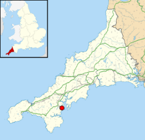
Fal estuary is located in the southwest of England. The
estuary is a ria (drowned river valley), and was formed
at the end of the last ice age, during which
glacial movement cut a channel through the area. Since
then, the sea level has risen by 120m (Bindoff et al,
2007) due to eustatic
change, resulting in the formation and subsequent
flooding of a river valley. The melting of the glaciers
after the ice age has resulted in isostatic rebound. The
removal of ice cover over Northern Europe has allowed
the land to rise, causing the south of the UK to sink. The
Fal estuary is located in the southwest of England. The
estuary is a ria (drowned river valley), and was formed
at the end of the last ice age, during which
glacial movement cut a channel through the area. Since
then, the sea level has risen by 120m (Bindoff et al,
2007) due to eustatic
change, resulting in the formation and subsequent
flooding of a river valley. The melting of the glaciers
after the ice age has resulted in isostatic rebound. The
removal of ice cover over Northern Europe has allowed
the land to rise, causing the south of the UK to sink.
The Fal estuary is
classed as a Special Area of Conservation (SAC). This is
mainly due to the high numbers of seagrass (Langston et
al, 2006) and maerl beds at St. Mawes bank, providing
important habitats for a number of species.
The Fal estuary is
macrotidal, with a mean tidal range of 5m and maximum
tidal currents below 2 knots.
In recent years,
dredging of the seabed has been proposed in order to
promote 'sustained long-term growth
of Falmouth’s cruise business'. As the increased traffic
may have an effect on the SAC, it is important to
understand the many different processes occurring within
the estuary in order to understand the full impact that
this dredging may have on the area.
Aim:
To gain an understanding of the physical, chemical and
biological processes in the Fal Estuary and the
surrounding coastal waters.
|
|
      
|
|
Equipment & Methods
|
|
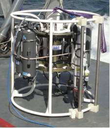
ADCP (Acoustic Doppler Current
Profiler) |
CTD
(Conductivity, Temperature, Depth) |
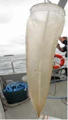
Plankton Net |
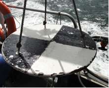
Secchi Disk |
|
The ADCP uses Doppler shift to determine current
velocity and direction. Particles within the
water body, such as zooplankton and suspended
particulate matter can also be detected from the
backscatter. |
The CTD measures conductivity (salinity),
temperature and pressure. The data is recorded
automatically on to the onboard computer. The
CTD frame can also be used to hold other
equipment such as; transmissometers,
fluorometers and Niskin bottles. |
Plankton nets can be towed behind the boat,
horizontal sampling or pulled up from depth,
vertical sampling. The net had a mesh size of
200µm. There was a flow meter recording the
volume of water which passed through the net. |
A Secchi disk is used to estimate the depth of
the euphotic zone. An observer lowers the disk
when the disk can no longer be seen is roughly
1/3 of the depth of the euphotic zone. |
|
 |
 |
 |
 |
|
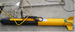
Subsurface SideScan Sonar |
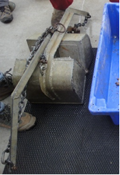
Van Veen Grab |
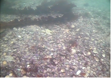
Video Camera |
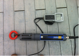
YSI Probe |
|
An acoustic pulse is emitted by the instrument
which reflects off the seabed and backscatter is
recorded. The intensity of the backscatter gives
indication to the make up of the seafloor. |
Grab used to sample the sea floor. Can be used
to give a sense of scale to the video recording.
Is a very localised sample and cannot sample
rocky areas. |
The waterproof camera allows pictures of the sea
bed to be studied, this can give a wider view of
the seafloor and is useful when used alongside
the grab |
Measures depth, pH, salinity, temperature,
chlorophyll a and DO2 % saturation.
The multiprobe is lowered into the water column
and readings were recorded every metre.
|
|
 |
 |
 |
 |
|
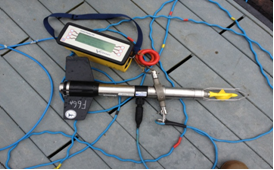
Valeport Current Meter |
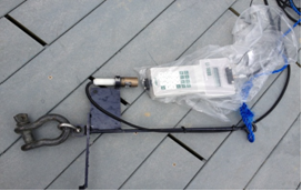
Li-Cor underwater PAR sensor, Li-Cor terrestrial
PAR sensor and Li-1400 datalogger |
|
Deployed in the water column, speed and
direction of current recorded at every meter. Works by measuring the speed of rotation of a
helix in the water. |
One sensor to remain dry to measure light above
water column. One sensor attached to weight to
measure light throughout the water column. Read
results from the data logger every meter. Units:
µmols-1m-2 |
|
 |
 |
|
Parameter to be
Investigated |
Method Applied |
|
Silicon |
Parsons & Lalli, 1984.
Stored in plastic bottles to avoid contamination. |
|
Phosphate |
Parsons & Lalli, 1984. Stored in glass
bottles to avoid contamination. |
|
Chlorophyll |
In-situ fluorometers and Welschmeyer method,
1994. Stored in glass bottles to avoid
contamination. |
|
Nitrate |
Flow Injection - Johnson & Petty, 1983. Stored
in glass bottles to avoid contamination. |
|
Dissolved Oxygen |
Semi-automated Winkler Method. Stored in glass
bottles to avoid contamination. |
|
Richardson (Ri) Number |
Ri number - indication of stability of water column
in estuary. When value<0.25, water column mixed - >1
it is stable (Knauss J, 1997). 0.25 - 1 indicates
shear instability. Ratio of static stability
(Brunt-Vaisala frequency) to the square of wind
shear.
 |
|
Phytoplankton |
Samples stained with Lugols solution and settled
overnight. Analysed under optical light microscopes
in 10ml samples |
|
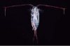
Zooplankton |
Formalin used to preserve sample. 2ml was
transferred to a Bogorov cell for examination under
a light microscope. |
|
|
 
|
|
Estuary
|
|
INTRODUCTION
Estuaries form an important transition
zone between saline marine environments and fresh riverine
environments, and their inherent physical, chemical and
biological properties help us understand the processes which
occur in the estuary. These semi-enclosed bodies of water
typically have high nutrient values due to the freshwater
input and therefore are zones of high productivity, making
estuaries a very dynamic and interesting area of study.
As two
groups were sampling, one in the morning and one in the
afternoon, this allowed them to
sample the river more intensely with one group (AM) focusing
on the upper part of the estuary and one group (PM) focusing
on the lower part of the estuary. This allowed for a higher
resolution when assessing the estuaries characteristics.
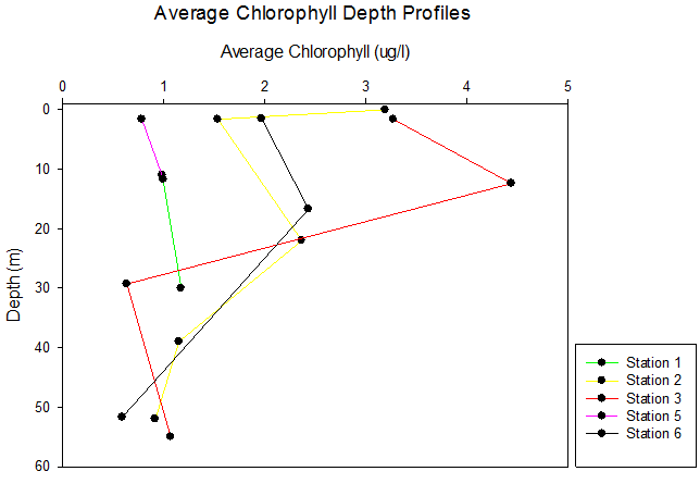
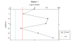
RESULTS
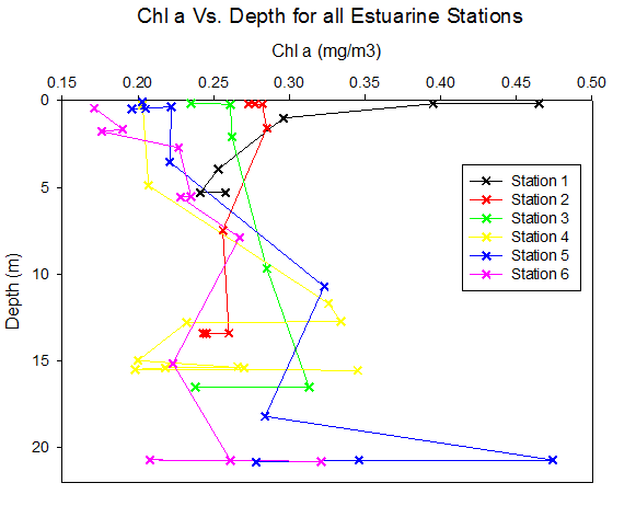
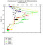
BIOLOGICAL - Chlorophyll
Station 1 has
two similar peaks at depths 3.5m and 1m. Due to the
sample area being shallow, deeper readings could not be
done. A strong decrease in chlorophyll concentration can
be observed at depths 2m and 5m. The 5m depth value at
station 1, being 0.456 µg/l, is one of the lowest
observed along the estuary. Only station 3 reaches a
lower concentration of 0.0846 µg/l at 6m depth. Station
3 chlorophyll concentrations peak to an overall highest
value of 2.154 µg/l at 12m. (Compared to studies by
Langston et. al 2003, these values seem significantly
lower. These studies showed measurements of around
20µg/l from the Truro river). From then on chlorophyll
concentrations drop again, indicating a decrease in
phytoplankton population density. Station 4 does not
have the same fluctuations as observed in all other
stations. Instead it has a slight increase in
concentrations, followed by a smooth decrease with
increasing depth. Station 5 had no depth recorded values
and hence only the surface value was recorded and
plotted. This may not allow for a full understanding of
the changes with depth, but one can observe the surface
changes of chlorophyll concentrations down the estuary.
Between stations 4, 5 and 6 there is a clear gradual
increase in surface chlorophyll concentrations, showing
that phytoplankton population increases at surface with
increasing distance down the estuary. At Station 6 high
chlorophyll can be observed at surface and at 5m. One
can observe a decrease of concentrations with depth.
Chlorophyll concentrations are dependent on various
factors such as oxygen concentrations, turbidity and
light intensity. Station 4 has a clear increase in
concentration, which correlates to oxygen concentrations
found at that site. Oxygen saturation decreases at
around 5-10m (Figure 7), which is the similar depth at
which chlorophyll rises in concentrations. This may be
due to chlorophyll respiration, causing oxygen depletion
(Johsnon et al., 2002). All stations experience
decrease of chlorophyll with depth, while oxygen
saturations show increases at 15m and beyond. This may
then be related back to the turbidity of the water
masses as well as light intensity. Looking at the
Richardson graphs (Figure 26) for station 4, one can see
that the water column is mostly turbid and well mixed.
High turbidity would cause phytoplankton to be mixed too
deep into the water column and hence reduce the amount
of light exposure (Cho, 2007). This close
correlation between chlorophyll and oxygen saturation
can also be observed at station 1 and 3. At station 3
the saturation rises with depth due to a decrease in
chlorophyll and station 1 has a clear fall-peak-fall
chlorophyll pattern in the upper 5m of the water column,
which matches the rise and fall of the oxygen saturation
at similar depths.
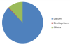
BIOLOGICAL - Plankton
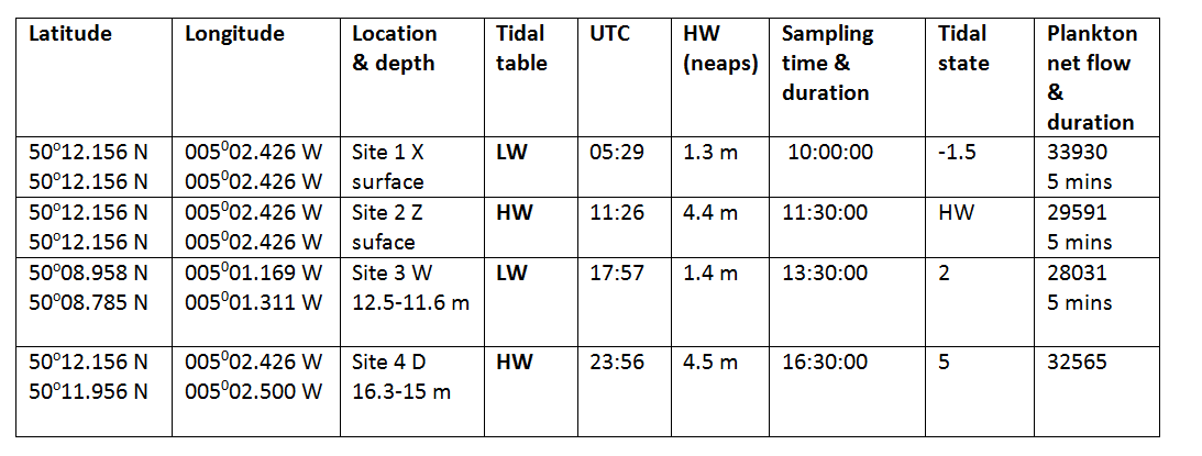
The Fal Estuary was sampled by two survey teams before
and after high water (HW) (Table 1). Overall
phytoplankton diversity was high with a greater
abundance of 640 cells/ml approaching HW compared to 99
cells/ml post HW. An overall diatom dominance of 87% was
typically representative of seasonal summer temperate
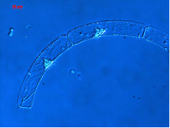
waters (Figure 1-3)(Kraberg et al., 2010; Widdicombe et al. 2009). Both
teams sampled phytoplankton at different depths and
dissolved oxygen % saturation measured as a proxy of
phytoplankton activity was lowest in the surface 10m
water column at most stations. This activity was
supported by a surface chlorophyll peak of 1-2 ug/L
above 10 m however these levels were below the UK
indicator value of 20 ug/L but above the 0.5 ug/L
suggestive of a bloom decline (Widdicombe et al.,
2010). It is suggested that the 210
µm mesh plankton nets sampled smaller diatoms
representative of an intermediate bloom succession
(Graph1)(Figure 4)(Langston et al., 2003).
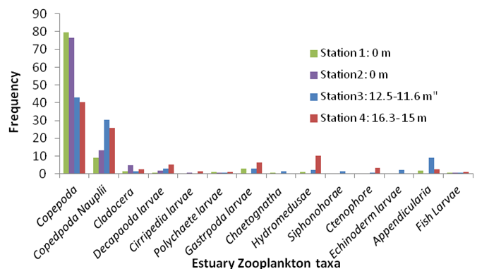
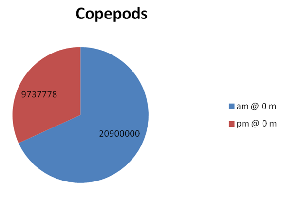
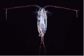
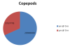
Heterotrophic holoplankton copepod and
meroplankton copepod nauplii
dominated both the estuary and offshore zooplankton.
Surface water zooplankton abundance of 1.0 x 10⁷
cells per m3 was more than double that
sampled in the afternoon suggesting lateral travel on
the ebbing tide to feed on phytoplankton prey (Figure
5)(Larick and Westheide, 2006).
Phytoplankton sampling was limited to deeper waters in
the afternoon and no night sampling was undertaken when
zooplankton use the protection of darkness to vertically
migrate to feed (Somerfield, Gee and
Warwick, 1994)(Figure 4 & 5).
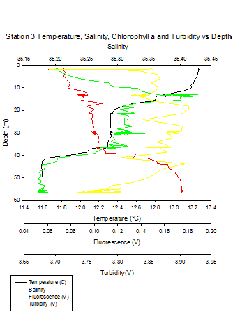
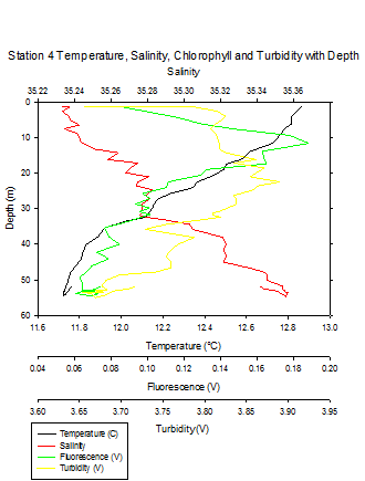
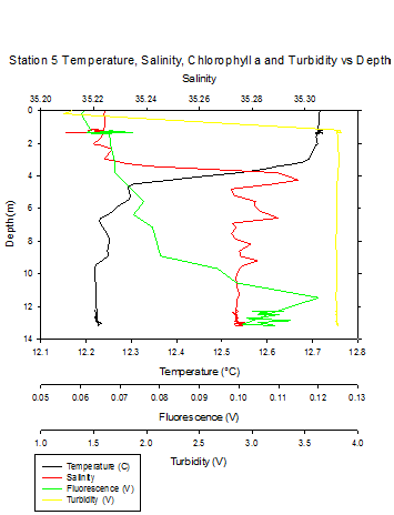
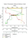
PHYSICAL - CTD
Figures 3a and
3b both give us insights into the vertical mixing
processes in the estuary. They both show an established
thermocline and halocline at station 1 - the station
highest up the estuary - which leads us to believe that
mixing in the upper section of the estuary is limited.
However, as you travel further down the estuary, the
gradient of the profiles decrease, indicating that the
mixing is increasing and causing the water column to
become more homogenous for both temperature and
salinity. Station 6 shows a well mixed, homogenous layer
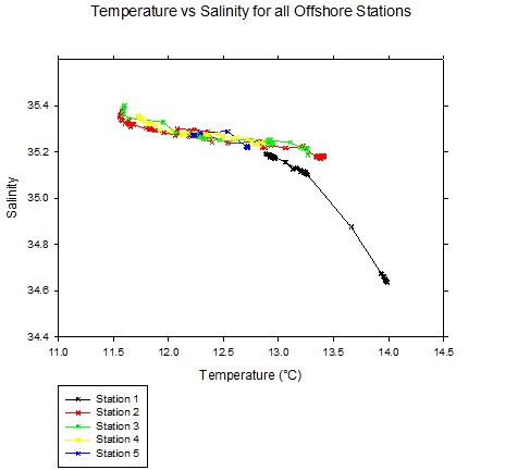
from surface to bottom. This is reflected in the T-S
plot (Figure 3c) which shows station 6 with a consistent
salinity and only a small change in temperature and
station 6 with a large change in both salinity and
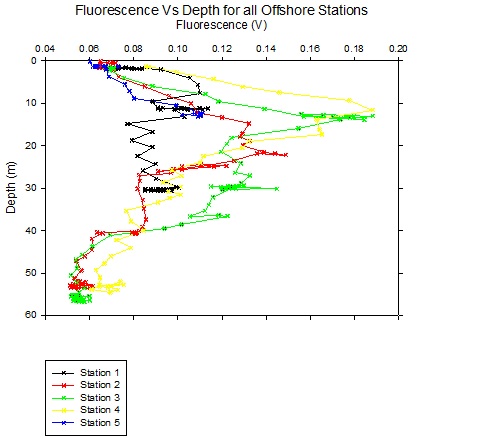
temperature. The fluorometer plot (Figure 3b) shows us
that surface levels of chlorophyll a decrease
from the riverine end of the estuary to the marine end,
and shows some possible formations of deep chlorophyll
maximums at the bottom/below the thermoclines.
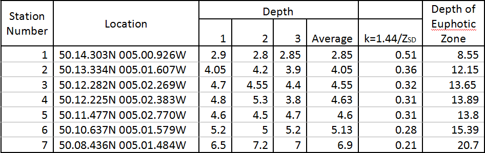
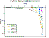
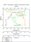
PHYSICAL -
Light Attenuation
The data shows that as you move down
the estuary towards the sea, the average secchi disk
depth increases from 2.85m (at station 1 – top of the
estuary)
to 6.9m (at station 7 – bottom of the estuary). The increase
in (ZSD) as you go towards the sea implies that
transparency of the water increases (or turbidity decreases)
as you move towards the sea. From average ZSD for
the stations, the euphotic zone depth was calculated and the
calculations show that the depth of the euphotic zone
increases moving towards the sea. The attenuation
coefficient decreases as you move towards the sea which
supports an earlier fact that the water becomes clearer as
you move towards the sea.
During the practical, it was observed
that the k decreases as you move toward the sea, meaning
that the secchi disk depth increases (because k = 1.44/ ZSD)
suggesting an increase in the transparency of water (or a
decrease in turbidity). This increase in transparency seems
to cause an increase in the concentration of chlorophyll in
the water column. The increase in chlorophyll concentration
in the water column is an indicator for an increase in
primary production. Increase in primary production is due to
the increase in depth of the euphotic zone, meaning light
penetrates further into the water hence, more phytoplankton
activity. Rivers and estuaries are usually higher in
turbidity than the open ocean; this is because river flow
rates are sufficient to cause material on the seabed to be
suspended in the water column. However, as the river reaches
the estuary, its flow rate decreases. The decrease in flow
speed causes deposition of material, therefore the
transparency of the water in the estuary increases as you
move down the estuary towards the sea, hence less light is
attenuated by the water column. And the depth of the
euphotic zone increases as less light is attenuated.
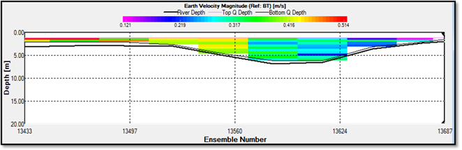
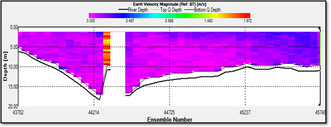
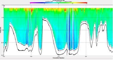
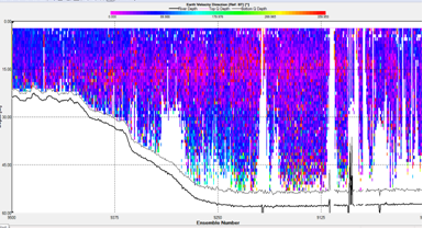
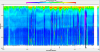
PHYSICAL - ADCP
Station one (Figure 6a) was the furthest up the estuary and
therefore had the shallowest water. At this station, the
depth of the water column does not exceed 10m. The
backscatter of the ADCP seems to increase from right to
left starting off with about 0.121 m/s, increasing with
depth to around 0.317 m/s – 0.416 m/s continuing to
increase with decreasing depth to flows of up to 0.514
m/s. It is a very gradual increase in flow velocities
that may be influenced, but not limited to, the small
increase in depth in the centre.
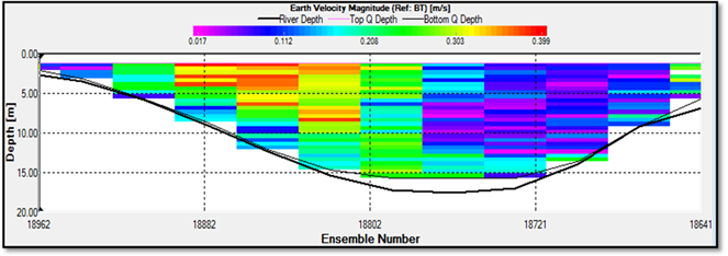
At station 2
(Figure 6b), the depth of the estuary increases
compared to station 1, however the pattern of increasing
flow from right to left still seems persistent. Overall
however, the flow is slower than previous. The right
hand side has flow velocities between 0.017 m/s to 0.112
m/s and increases to values of about 0.399 m/s on the
left. To the far left of the transect backscatter
decreases again. The highest flow rates can be observed
closer to the surface, whereas the bottom waters have a
generally calmer flow between 0.208 m/s and 0.303 m/s.
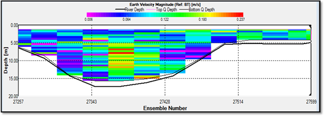
Station 3
(Figure 6c) has no obvious patterns
as previously observed. It appears to be slightly more
uniform, where flow velocities lie in the range of 0.064
– 0.122 m/s. The flow seems a bit increased at the right
of the transect, where depth decreases. At about 10m in
the centre of the transect, there is a very obvious
increase in backscatter showing an increase in velocity
of the water masses present there. The increased
velocity ranges from about 5-12m and has flow rates up
to 0.237 m/s. Although high, it is not as high as
previously observed values at station 1 and 2. The flow
seems to decrease slightly towards the left of the
transect.
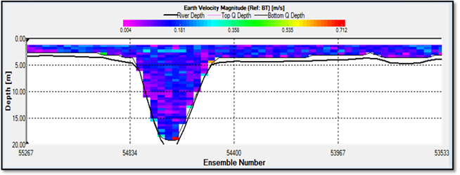
At station 4
(Figure 6d) the water mass seems
to have roughly the same velocity throughout the
transect, with values ranging between 0.004 – 0.181 m/s.
At the left of the transect a small patch of decreased
backscatter can be observed, showing a decrease in flow
velocities. The ADCP shows a deep caving, which is the
beginning of the deep channel that runs through the Fal
estuary. In there the flow rates seem to have decreased
slightly. Surface waters in general are uniform, with
quite similar velocities throughout the transect
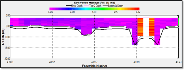
Station 5
(Figure 6e) shows a blank spot which represents
the deep channel that runs through the Fal estuary. Due
to its depth being beyond 20m, the ADCP was not able to
do any recordings. There was overall low backscatter
recorded. The ADCP shows an up cropping bed form feature
on the right and left of the deep channel. At that point
the flow velocities recorded increase from around 0.010
m/s to 2.752 m/s. These velocities are still not as high
as those observed in station 1. In general the surface
waters seem to have a slightly higher flow rate than the
bottom waters
Station 6
(Figure 6f) similar to station 5, the flow
around the opening of the deep channel is low, at values
of around 0.005 m/s. It also shows a small up crop that
causes an increase in the water flow to 1.972 m/s.
Towards shallower waters the backscatter increases
showing a slight increase in flow rates. In general the
surface waters seem to have a slightly higher flow rate
than the bottom waters. To the left of the transect the
water has a slower flow than to the right. The water at
station 6 is deeper than at station 5
As the 2 groups conducted their
survey at different parts of the day (AM and PM) and
high water was at 11:24, we can see the tidal velocity
profiles of the estuary for the incoming flow tide in
the morning (station 1-3) and the outgoing ebb tide
(station 4-6) in the afternoon. As the tide at the top
of the estuary is mesotidal, we can see that the tidal
currents have less velocity than those at the bottom of
the estuary, where the tide is macrotidal. These tidal
currents and their magnitudes have a large effect on the
physical structure of the estuary.
The ADCP on the boat can sometimes
give us spurious results due to a number of different
factors. Firstly the chop from the engine can cause air
bubbles to form at the surface, changing the way that
the ADCP sonar waves travel through the water and
creating noise on the velocity and backscatter plots.
Secondly things can block the ADCP sonar. For example at
stations 5+6 you can see a lack of data in the channels
in the estuary. This could possibly be due to the ADCP
being taken during the CTD drop and obstructing the ADCP
sonar.
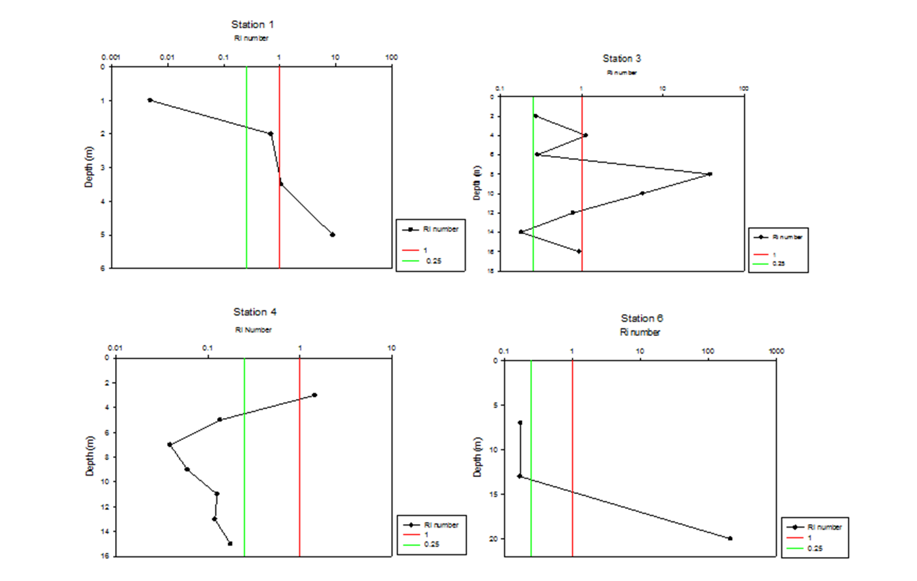
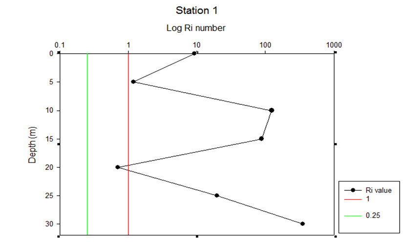
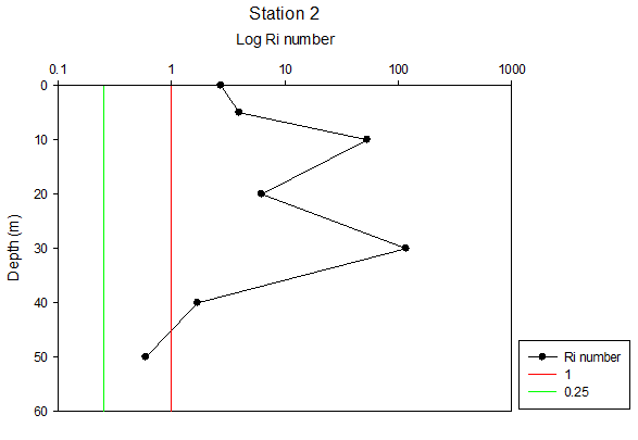
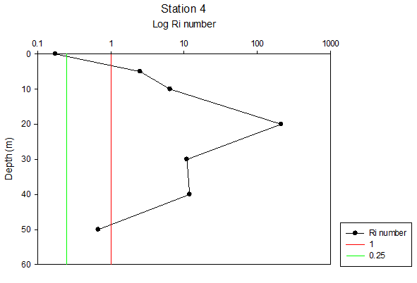
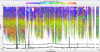
PHYSICAL - Richardson Numbers
The Richardson number is a good
indication of the stability of the water column in the
estuary. As the CTD salinity measurements on the Conway
vessel were not correctly calibrated, the salinities
measured in-vitro were used to calculate the densities
of the samples taken to analyse the chemical composition
of the estuary. The densities were used to calculated
Richardson numbers. This is why our Richardson numbers
are only calculated for certain depths, and not at all
for stations 2+4 (no water samples were taken on these
drops).
Station 1 has a transition from strong mixing waters
with Richardson values below 0.25 into stable water flow
of Richardson values above 1. Between 2m and 3.5m the
flow resides in the area between 0.25 and 1, indicating
shear instability. The water flow in the top 2m of the
water column has low Ri numbers which show that there is
strong mixing. Between 3-5m one can see the decrease in
flow and hence a decrease in mixing. The point at 2m
could be an indication of the position of the
thermocline, as the flow rate decreases causing
stratification.
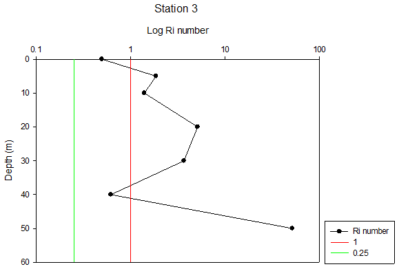
Station three had more samples taken than station 1 and
so it was possible to create a clearer depth profile.
Between 2-6m the values lie perfectly in the area
between 0.25 and 1, indicating low mixing and the flow
will be dependent on temperature and density. At 8m
depth there is a high peak in the values, where the flow
becomes stable and less mixed. The stability of the flow
gradually decreases again as depth continues to
decrease. The values then maintain themselves in the
area between 0.25 and 1, again indicating well mixed
waters. The middle can be assumed to be stratified and
surrounded by two well mixed layers of water.
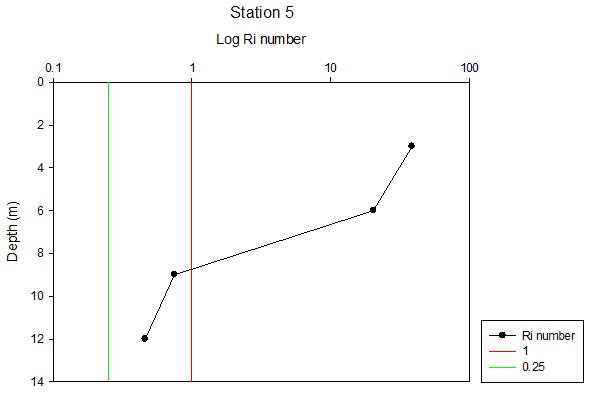
Station 5 shows decreasing Richardson number with depth
in the top few metres, and slight increase beyond around
7m. The vast majority of the water column had a Ri of
below 0.25- indicating a turbulent water column. At
around 4m depth the flow lies in the area between 0.25
and 1 indicating that the flow is dependent of density
and temperature. Stratification occurs in the surface
layers due to thermal heating, forming a thermocline.
Station 6 appears to show turbulent surface waters, with
Ri of less than 0.25 and gradual stratification with
depth beyond around 13m. At around 20m the Ri is over
100, indicating a strongly stratified water column. One
can assume the water column experiences a transition
period, shown by the area between 0.25 and 1, which may
be due to a thermocline.
PHYSICAL - Residence Times 
The
residence time of the Fal estuary was calculated by
using the formula:

The mean
estuarine salinity was calculated from all recorded
values from station 1 through 6 (see table 2).The sea
salinity was the marine end member recorded using a CTD
at station 6. The total volume of the Fal is roughly
1.35×10⁷ m3. In order to find the
discharge rate into the Fal, data was obtained from the
Centre for Ecology and Hydrology. The database had daily
readings of discharges into the Fal estuary since 1978.
For the purpose of this investigation data from 2000
-2010 was used, allowing for a 10 year average (see
table 3).
|
|
Station 1 |
Station 2 |
Station 3 |
Station 4 |
Station 5 |
Station 6 |
|
Salinity |
25.8 |
31.2 |
32.3 |
35 |
33.9 |
34.5 |
Table 2 - Salinity values
recorded at each station along the estuary
Average Salinity is hence: 32.12
|
Year |
Salinity |
|
2000 |
2.98 |
|
2001 |
2.09 |
|
2002 |
2.33 |
|
2003 |
1.64 |
|
2004 |
1.76 |
|
2005 |
1.49 |
|
2006 |
1.48 |
|
2007 |
1.97 |
|
2008 |
1.94 |
|
2009 |
2.21 |
|
2010 |
1.59 |
|
Average |
1.95 |
Table 3 – Average yearly
discharge into the Fal from 2000 to 2010 and the final
average value for the 10 year range
One should
note that the values provided from the Centre were from
the Fal at Tregony, which is beyond the point of
sampling. Hence the calculated value may actually be an
understatement of the actual residence time, due to lack
of sampling further up the estuary.
The calculated
residence time for the Fal estuary is hence:

The Fal
estuary has a fairly short residence time, allowing for
incoming pollutants and other harmful substances to be
flushed out and allowing for uncontaminated water to
come in.
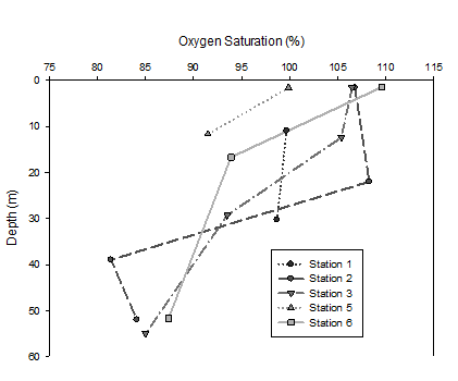
CHEMICAL - Oxygen
Most stations show an increase in
saturation at a certain depths, stations 1 and 4 show this
increase in the first few metres, whereas station 3 shows an
increase around 10m. Station 6, the most marine station
shows a slight decrease with depth, however a surface value
is absent due to error and a mid-depth value is
significantly higher, suggesting an anomaly.
Oxygen concentrations are strongly influenced by
phytoplankton abundance and blooms. Due to respiration
phytoplankton will cause a decrease in oxygen
saturation. Oxygen saturation decreases at around 5-10m,
which is the similar depth at which chlorophyll rises in
concentrations (see chlorophyll analysis – estuary). The
saturation of oxygen can either rise or fall with depth.
Rising would indicate a well-mixed water column, where
surface oxygen is mixed to deeper layers. A fall in
saturation could occur due to lack of replenishment to
the depth. Concentrations of oxygen can also be impacted
by high amounts of bacteria caused due to pollution. It
is known that the Fal Estuary has major mining
discharges into it, containing heavy metals that impact
the biology as well as chemistry (Bryan, G. and
Gibbs, P. 1983). One can see that oxygen saturation
is fairly low at the top of the estuary at station 1.
This could be due to eutrophication leading to high
amount of bacteria, which would consume the oxygen in
the upper water column and change the chemistry
(Jorgensen and Richardson, 1996). It would cause a
change in biological composition of the water. The
oxygen saturation depth profiles can be more of a
representation of the seasonal cycles of nutrients and
chlorophyll, such as seen in station 4 (see chlorophyll
analysis - estuary).
CHEMICAL - Silicon
The composition of
estuarine waters varies considerably, depending on the
main source of dissolved salts (Olaussan and Cato 1980
p-72). Dissolved constituents that enter the estuary
behave in accordance to the physical and geochemical
characteristics of the estuary. For some constituents
the estuary is a simple chemically conservative mixing
interface between the rivers and the ocean (Loder and
Reichard 1981). For others the estuary is an environment
that acts as a reaction vessel, resulting in substantial
depletion and addition.
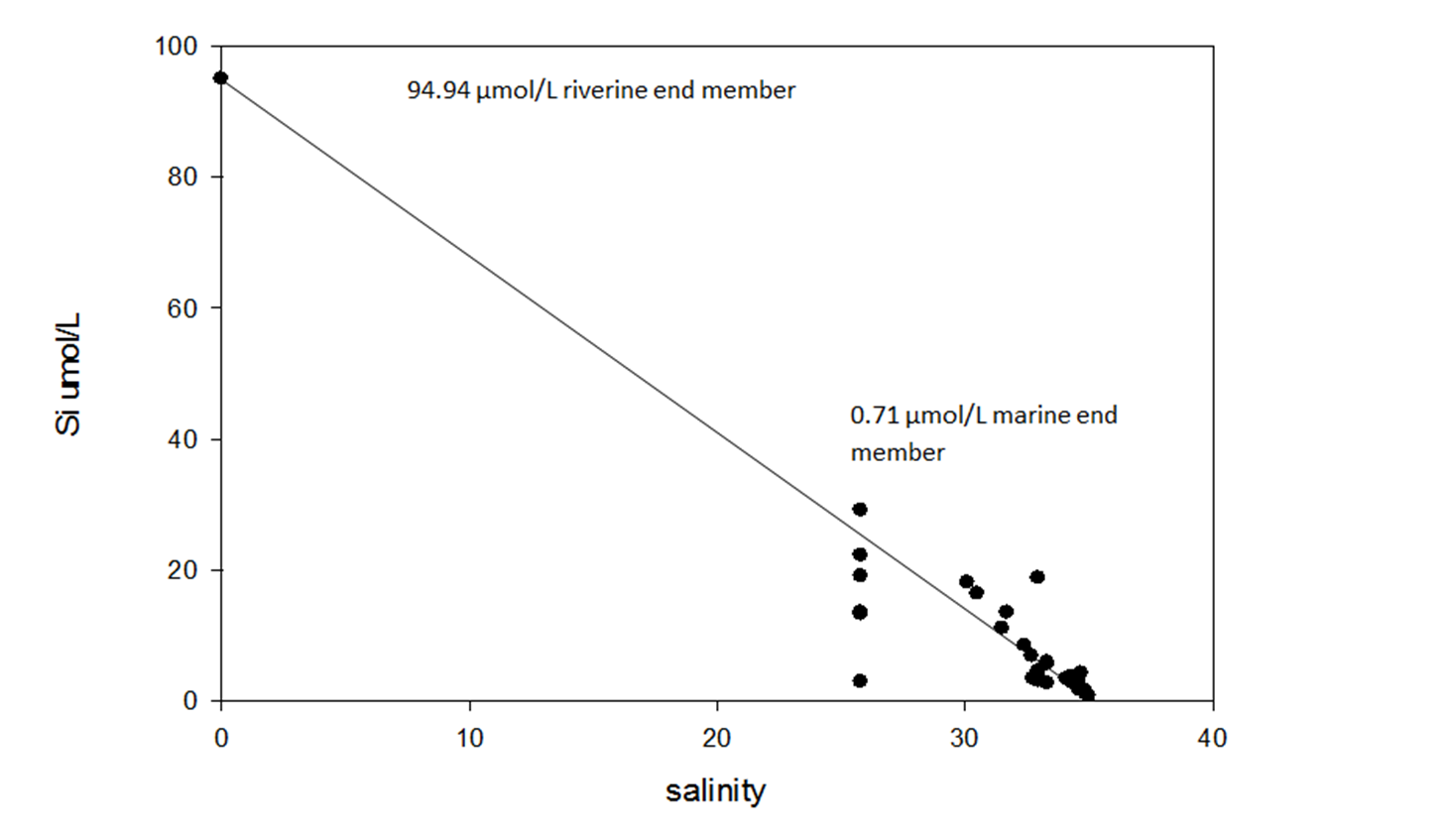
Figure 8 displays
the behaviour of dissolved silicon
Si(OH)4
in the lower part of the Fal estuary. Silicon is a key
dissolved constituent in estuarine environments and is
often correlated with phytoplankton production. Diatom
populations are particularly vulnerable to silicon
fluctuations because they require silicic acid to
produce external skeletal material. Thus considerable
variation in silicic acid concentrations can determine
the dynamics in phytoplankton communities and regulate
the amount of primary production in a given estuary.
When diatom blooms occur in the spring and autumn when
irradiance levels are sufficient for substantial for
primary production, silicon concentrations plot below
the theoretical dilution line (TDL), which indicates the
dissolved constituent, is behaving non-conservatively.
Substantial addition to the environment from
anthropogenic or from naturally occurring physical
processes can also result in non-conservative behaviour.
In this case silicon concentrations will congregate
above the TDL. Conversely when silicon values display
linearity it is said to behaving conservatively i.e.
dissolved silicon is behaving in relation to the
physical mixing between the riverine and marine end
member.
In this case samples
collected from the lower end of the Fal estuary are
behaving conservatively (R2= 0.9992),
typical of a well-mixed estuary. Values are
extremely low which is to be expected in the lower part
of the estuary where any external addition of silicon is
negligible and quickly diluted. Despite strong
correlation there seems to be a possible outlier (i.e.
an anomaly in the data set) at salinity value 34.7. Despite thorough preparation and
data handling control human error is inevitable possibly
skewing the data set. The riverine end member was
collected prior to the investigation from the Truro
tributary and was multiplied by 5 because of the
dilution factor, yielding the true concentration. The
marine end member was taken from the concentration at
the highest salinity in this case 0.71mmol.
Conversely
Silicon values found in the lower estuary lie above the
theoretical dilution line, which suggests that silicon
is behaving, non-conservatively (R2=0.8679).
Values found between 30.1- 32.4 lie above the TDL, which
suggests that silicon is been replenished from an
external source, possibly from the various tributaries
that flood into the estuary. Possible anthropogenic
impacts from sewage run off could also cause
fluctuations in dissolved constituents in the lower part
of the estuary. Beyond >32.4 Psu silicon becomes
depleted, which suggest biological utilisation in the
intermediate salinities. However all these assumptions
are based on a steady state environment, ignoring
Flushing time and residence time values (in this case 7
days for the Tregony river). Also the relatively low
freshwater inputs from the six main tributaries maintain
high salinity values, which explains why all the samples
were collected between 25- 35 psu. Thus the
interpretation of theoretical dilution diagrams must be
undertaken with an understanding of the variability in
behaviour of dissolved constituents and their
relationship to the mixing properties and flushing times
(Loder and Reichard 1981).
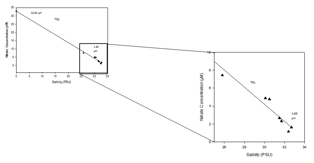
CHEMICAL - Nitrate
Conservative
behaviour shown by Nitrate along the estuary, general
structure shows a decrease in concentration of Nitrate
with an increase in Salinity. Data points follow TDL,
which doesn’t indicate any addition or removal of
nitrate. When comparing riverine end member
concentrations with Langston et als (2003) nitrate
concentrations in the Kennal and Truro river, our
calculations show significantly lower nitrate
concentrations than theirs. In order to convert their
values in mgl/l to µmol/l we had to use the molecular
mass of presumably NO3 (unsure of whether
Langston et al used nitrite or other). From their
report, the Kennal river displayed values of 83mg/l
compared to our end member concentrations of 32.83mg/l
which is significant difference. This lower value could
be due to long period of rainfall over the past few
weeks, which has “diluted” the nitrate within the
estuary.
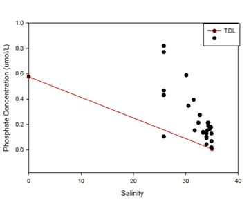
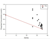
CHEMICAL - Phosphate
Figure 11b shows how phosphate
concentration varies across the Fal Estuary. The
concentrations of the marine end member and the river
end member are 0.0073umol/L and 0.5770umol/L
respectively. The figure only shows a partial picture of
the Fal Estuary, this is because concentrations for
lower salinities were not obtained, and the lowest
salinities recorded were 25.8. As a result of this, the
river end member was provided at the lab. From Figure
10a can observe that the data point do not plot on or
close to the theoretical dilution line (TDL), the all
data points save one, lie above the TDL, this means that
phosphate is added into the system as you move toward
the sea (higher salinity end). This addition of
phosphate means that it behaves in a non-conservative
manner (conservative behaviour means that it will plot
along the TDL).
To allow us to
compare our values with other reports on the estuary, we
had to convert our phosphate concentrations firstly to
orthophosphate and then from µmol/L to mg/L using the
molecular mass of the compound.
Comparing the riverine end member to Langston et al
(2003) various orthophosphate concentrations in the
Truro River, our end member appears to be lower than the
orthophosphate concentrations in the Truro River, which
are 0.1mg/l, whereas from our calculations we calculate
orthophosphate concentrations of the end member to be
0.04mg/l. Looking at Langston et als other river
concentrations our results show a low concentration of
orthophosphate in the estuary, however it is still
within the limits calculated by Langston et al.
Discussion:
The addition of phosphate into the
system could be attributed to the fact that there is
more than one river input into the system for example;
River Fal, Truro River, Percuil River and Mylor. The
inputs from these rivers are likely to add phosphate
into the system due to the number of rivers and
tributaries into the estuary.
Phosphate concentration can be
affected what is happening at the sediment boundary.
Changes in weather and sedimentation rates in the short
term could affect the concentration of phosphate in the
water temporarily. If there was a storm in the area,
wind speeds and flow rates would be higher in the area.
This means that there is more input into the estuary and
higher wind speeds could stir up the sediments at the
estuary bed and release nutrients into the water hence
increasing the concentration of phosphates in the Fal
Estuary.
The pH of the water could also be
the cause of the addition of phosphate in the lower
estuary. Adsorption is highest when pH is 3 – 7.
Therefore, adsorption rates should decrease as you go
towards the sea as the pH for seawater is about 8.
Concentrations of phosphate varies
annually, it is observed that concentrations are highest
in the summer. Phosphates are remineralized as it reacts
with iron to form ferric phosphate which is insoluble.
As summer progresses, the estuary becomes more anoxic
due oxygen consumption being greater than oxygen
production rates (from phytoplankton), this improves the
rate of reduction of iron, which releases phosphate from
ferric phosphate into the water. This would cause an
addition of phosphate in the estuary.
CONCLUSION -
Estuary
The data collected within the Fal
estuary contains biological, chemical and physical
parameters. The transition between different parts of
the estuary was observed using the data collected.
Surface levels of chlorophyll were
found to decrease from marine to the estuary end, the
nitrate decreases towards the marine end and has been
seen to been added to the water in the riverine end due
to anthropogenic inputs. Turbidity increases with
increasing salinity due to reduced flow speeds resulting
in natural deposition of suspended material. Phosphate
addition occurs most in the summer periods. Addition
occurs due to inputs from more than one river and also
oxygen production rates, reducing iron so added ferric
phosphate to the water. All these can be affected by the
spring plankton blooms. The zooplankton was dominated by
copepod and copepod nauplii. Silicon behaves
conservatively in the estuary and shows addition this
can also be due to anthropogenic inputs.
The ADCP was essential in assessing
the level of stratification in the estuary, indicated by
the calculation of Ri numbers using the velocity
magnitude. It also helped us understand the tidal
processes in the estuary, helping us evaluate the impact
of the tides on the vertical and horizontal structure of
the estuary.
The depths of the estuary samples were quite shallow so
making detailed depth profiles difficult.
|
|
Date |
28/06/2012 |
|
Location |
Fal Estuary |
|
Wind |
F2 SW |
|
Tide |
1124 |
|
Weather |
Sunny |
|
Sea State |
Calm |
(a)
  (b)
(b)
Figure 1a-b
: (a) The Fal
Estuary and its tributaries (b) study transects across the
estuary.
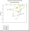
Figure 2 - Average chlorophyll values
calculated for each site depth profiles (Station 1 being the
furthest up the estuary and Station 6 furthest down.)
(a)

(b)
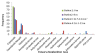
Figure 3a-b: (a)
Fal Estuary survey times, locations, duration and depth with
a local tidal table indicating high water (HW) and low water
(LW); (b)
Estuary am (site 1 &2) and pm (site 3 & 4) zooplankton taxa
(c)
  (d)
(d)
(e)
  (f)
(f)
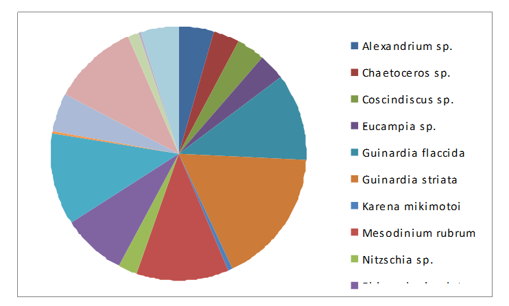
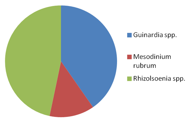
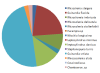
Figure
3c-f: (c) Phytoplankton taxa; (d) Dominant Fal estuary
phytoplankton; (e) Fal estuary phytoplankton species; (f)
Copepod abundance am and pm in Fal estuary
(a)
 (b)
(b)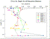
(c)
  (d)
(d)
Figure 4a-d: (a) Estuarine Salinity-Depth
Plot; (b) Estuarine Chlorophyll-Depth Plot; (c) Estuarine
Temperature-Salinity Plot; (d) Estuarine Temperature-Depth
Plot

Figure 5
- Table showing averaged Secchi disk depths, attenuation
coefficient, and depth of euphotic zone at each station.
(a)
  (b)
(b)
(c)
  (d)
(d)
(e)
  (f)
(f)
Figure
6a-f: (a) ADCP Transect 1; (b) ADCP Transect 2; (c) ADCP
Transect 3; (d) ADCP Transect 4; (e) ADCP Transect 5; (f)
ADCP Transect 6
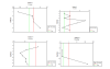
Figure 26.
Ri for Station 1,3,4 and 6.
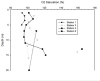
Figure 7 - Oxygen
saturation depth profile for the estuary (Stations 1, 3, 4
and 6). Anomalous points for stations 3 and 6.
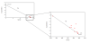
Figure 8a.
Lower Estuary Silicon Theoretical Dilution Line (TDL)
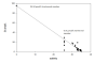
Figure 8b.
Estuary mixing diagram
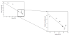
Figure 10. Nitrate mixing diagram for
Fal Estuary plus close-up.
(a)
  (b)
(b)
Figure 11a-b:
(a) Phosphate against absorbance; (b) Phosphate depth
profile
|
|
 
|
|
Offshore
|
|
INTRODUCTION
Vertical mixing in the water column has
a large influence on primary production in the ocean.
During the seasons, variation in mixing processes will
regulate the nutrient concentration in the surface layer of
the ocean. For example during the summer months, the
increase in solar radiation and the strengthening of the
thermocline will lead to an increased level of phytoplankton
production, in turn leading to depletion of nutrients in the
area (e.g. Silicon and Nitrate). The degree to which the
nutrients can be replaced will depend primarily on the
amount of vertical mixing that will occur, drawing up
nutrient rich water from deeper depths.
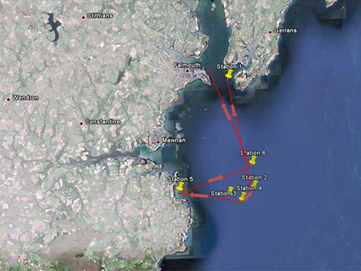
Our investigation was carried out on
six stations in the western English Channel. Weather
constraints (high winds leading to rough seas) prevented us
from sampling areas further out into the channel, and
therefore we sampled closer to the coast than initially
expected (see Figure 12).
Each station consisted of a CTD drop
and an ADCP profile, from which we analysed the water column
structure and decided whether to deploy Niskin bottles to
collect water samples and at what depths. If deemed
necessary, the Niskin bottles were fired as the CTD
ascended. The samples were then analysed at a later date in
the lab where we tested for plankton abundance and species
composition, nutrient concentration of N,Si and P, oxygen
concentration and chlorophyll a.
RESULTS
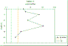
Biological -
Chlorophyll
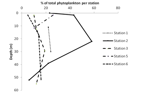
Station 1 only had two depths sampled,
hence not giving a detailed overview of the depth profile.
However, it indicates a slight increase between depths of
11m to 30m. Station 2 shows high surface values which
overall decrease with depth. A small peak can be observed at
22m, however the chlorophyll concentration at depth does not
reach that of the surface values. Station 3 has a similar
surface value to station 2, however at about 12m it peaks to
the overall highest recorded concentration of 4.4 µg/l. The
peak is followed by a sharp decline in concentrations as
depth increases. Station 5 is a rather low chlorophyll area,
having the overall lowest values recorded at surface. As
with station 1 it does not allow for a detailed depth
profile, but does indicate a slight increase with depth.
Station 6 does not have fluctuations as strong as station 2
and 3. Chlorophyll concentrations increased slightly until
around 16m, where after they fall to similar values of that
found in other stations. Where it was possible to take
samples of 50m depth or more the values of chlorophyll are
fairly similar, showing an overall similarity of
phytoplankton population distribution past certain depths.
Chlorophyll concentrations are
dependent on various factors such as oxygen
concentrations, turbidity and light intensity. Station 2
shows a correlation with oxygen saturation seen in
Figure 20. At the very surface of the water column,
concentrations drop and only increase again at depths of
30m. The oxygen saturation increases at the surface does
the exact opposite to chlorophyll; it decreases at
around 30m. This is due to respiration of the cells
causing depletion of oxygen. The small peak in depth at
station 2 may also be enhanced by the very light peak in
irradiance that can be observed in Figure 25 at depth of
about 15m (Violette, 1995). The low chlorophyll
values observed in station 2 at surface may also be
related to the stable flow of the water, indicated by
the Richardson number (Figure 17). Station 1 indicates
low chlorophyll values, which can most likely be related
to high stratification at those sights also due to high
Richardson numbers. High stratification would cause a
gradual nutrient depletion of the top water column and
hence a lower concentration in chlorophyll.
Station 2- possible frontal system with two observed
maxima, one at the surface and a second at 16m. This
correlates with high backscatter recorded from the ADCP
data at station 2 (Figure 16b) which is indicative of a
tidal front system. Furthermore high levels of
zooplankton were observed between 25-15m suggesting
strong stratification at station 3, which correlates
with the deepest chlorophyll maxima observed from the 6
stations. The stability of the water column increases
the critical depth and depending on the irradiance
intensity and turbidity of the water column, there will
be a net gain in photosynthesis, thus producing
chlorophyll maxima at depth.
BIOLOGICAL -
Plankton
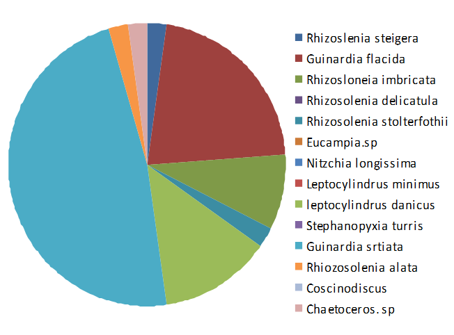
The most dominant taxa of diatom found in the offshore
practical was Guinardia sritiata. The overall
total of the samples contained 48% of this species. The
least dominant taxa found were Eucampia sp,
Leptocylindrus minimus and Stephanopyxia turris
each having only 2% of the overall total of
phytoplankton. Guinardia sritiata was also the
most dominant species at station 1, 2 and 6, however at
station 3 Guinardia flacida was most dominant and
at station 5 Rhizosolenia delicatula was most
dominant.
The chlorophyll maximum at station
2 corresponds with the peak in phytoplankton: 58% at a
depth of 23m (seen in Figure 14c at station 2). This also corresponds with the
lowest reading a phosphate for the same station at the
same depth. At station 2 there is a sharp decrease in
phytoplankton from 58% at 23m to 5% at 52m, showing a
possible nutricline.
There
were very low numbers of dinoflagellates counted at the
offshore stations, (6 counted in total for all the
sites) possibly due to being consumed by the large
amounts of copepods that were present.
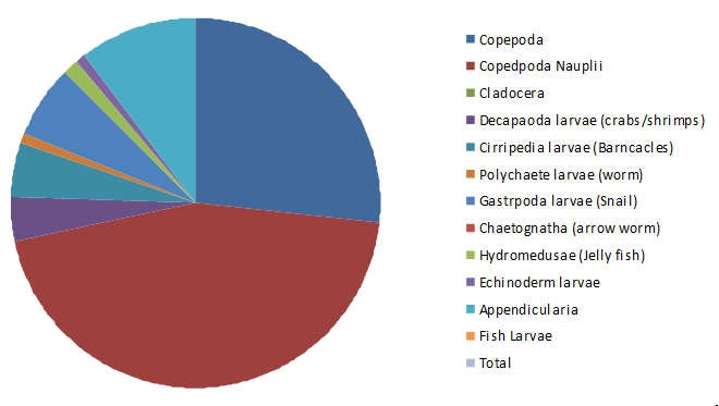
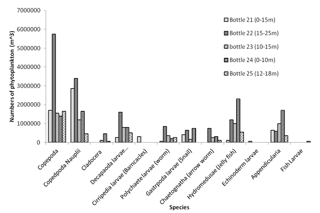
The most dominant species of zooplankton were the
copepod and the copepod nauplii with an abundance of 45%
and 27% respectively. The least abundant zooplankton
found was fish larvae. The highest numbers of copepods
were found at depths of 12-18m at station 6 and 15-25m
at station 2; both these stations were furthest from the
land. Copepod nauplii were most predominantly found at
station 1 between 0-15m and station 1 was located close
to land. The chlorophyll maximum was found between 11
and 22m at all the stations, this is also where the
majority of the copepods were found.
Diatoms together with planktonic algae provide good
nutrition for the copepods. High diatom abundance can
have a negative effect on copepod reproduction (Nejstgaard,
et al (2001)). Copepod nauplii were found in higher
abundance in areas away from the higher numbers of
diatoms. Higher nauplii production occurs when there are
blooms in a flagellate bloom, the flagellate numbers
were extremely low.
Tidal fronts dominate shallow seas around the UK. They
are dominated by diatom blooms and are marked by a
chlorophyll maximum layer at the subsurface. (Franks,
1992). The chlorophyll maximum for the highest
concentration of chl α was found at site 3 at a depth of
15m. The second highest was at site 2 and corresponds
with a high count of copepods and a high count of
phytoplankton. This is also the depths with the lowest
phosphate and increasing amount of nitrate so this could
indicate the presence of a front between sites 2 and 3.
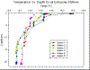
PHYSICAL - CTD
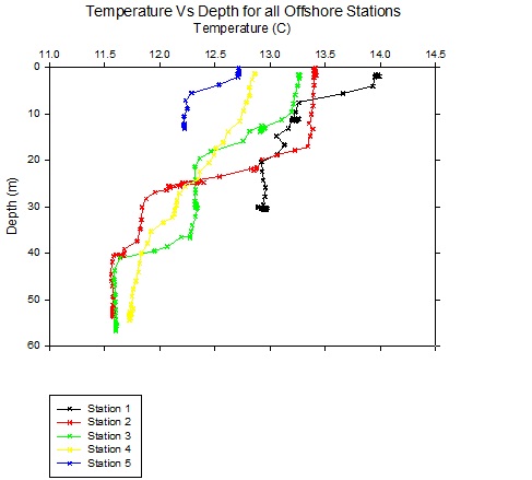
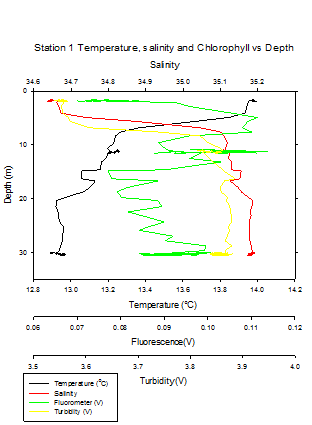
Station 1 (figure 15e)- Temperature
changes from nearly 14⁰C to 13.2⁰C between 5 and 10m
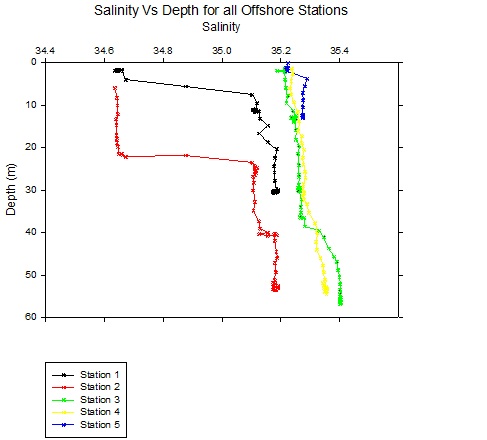
depth, relatively shallow thermocline. Salinity
increases from 34.65 to 35.10 as temperature falls at
the thermocline, halocline corresponds with thermocline,
then salinity remains between 35.1 and 35.2 at greater
depths. Turbidity increases at the lower depth of the
thermocline. The fluorometer shows a Chlorophyll a max
at 0.11V between 5 and 8m depth with a large sharp peak
at 11m of the Voltage.
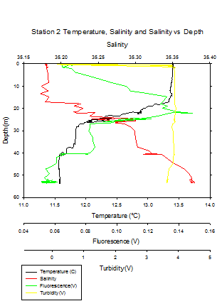
Station 2 (figure 15f) -
Thermocline is deeper, temperature falling from 13.5⁰C
to 11.7⁰C between 20m and 28m then there is a small
decrease from 11.7⁰C and 11.5⁰C between 38 and 40m
describing a stepped thermocline. Fluorometer shows
chlorophyll steadily increases from surface to 18m, chl
max shown as 0.15V between 18 and 23m. Fall in chl down
to 0.08V from 23 to 28m and decrease in chl at 40m from
0.08V to 0.06V. Decrease of temp at thermocline
corresponds to increase of Salinity. Turbidity jumps
around between 0V and 4Vin the surface 1m as the CTD is
lowered and swashed by swell. Turbidity peak at chl max
of 3.94V.
Station 3 (figure 15g) - Strong
thermocline between 10m and 20m and with a well mixed
section between 20m and 37m with a second strong
thermocline shown with temperatures falling from 12.3⁰C
to 11.6⁰C between 38 and 40m. Chl peak of 0.18V at 15m,
remains relatively steady between 20 and 38m and falls
from .12V to 0.06V from 38 to 40m. Turbidity peaks at
lower thermocline depths although only small changes in
turbidity observed. Salinity increases slowly from 35.2
at the surface to 35.26 at 38m then increases more
substantially from 35.26 to 35.4 between 38 and 50m.
Station 4 (figure 15h) - Well mixed
upper water column with a reasonably consistent decrease
in temperature from 12.8⁰C to 11.8⁰C between the surface
and 50m. Shallow chl max of 0.18V at 10 to 12m and
gradual decrease of chl to 0.10V at 25m, chl remains the
same between 25 and 32m then decreases to 0.06V at 50m.
Salinity increases uniformly from 35.24 to 35.28 between
0m and 25m, remains at 35.28 between 25 and 33m then
increases with depth with a brief steady period at 35.32
between 38 and 45m. Turbidity is highest (3.9V) at 22m,
decreases to 3.73V between 22m and 35m, turbidity higher
in surface 30m.
Station 5 (figure 15i)- Shallow
thermocline between 2.5m and 4m where temp changes from
12.7⁰C to 12.3⁰C. Salinity shows an increase between
2.5m and 4m from 35.22 to 35.28. Chl increases slowly
from a 0.06V reading at the surface to 0.08V at 8m then
increases more rapidly with depth from 0.08V at 8m to a
peak of 0.12V at 12m. Turbidity shows an even value of
3.8V through the analysed water column. Surface
turbidity change here describes the CTD entering the
water.
Discussion
Thermal
Stratification is a key aspect of offshore waters in
early July. Increased solar radiation during the summer
months increases solar radiation absorbed by the oceans
resulting in increased warming of surface waters. Warmer
sea water is less dense than cold sea water of the same
salinity. Surface waters therefore increase in buoyancy.
Thermal stratification occurs when the increase in
buoyancy is strong enough to overpower vertical mixing
of the water column. A stable warmer surface layer is
formed, distinguished from the rest of the water column
by a region of rapid temperature change, the thermocline
(Smythe et al. 2009).
The most
striking difference in the data displayed above is the
levels of stratification experienced at the different
Stations. Stations 2 and 3 are furthest offshore and
show far deeper thermoclines (Figure 15a) indicating
stronger thermal stratification. The thermocline at
Station 5 for example is found between 2.5 and 4m due to
disruption of formation of thermocline by tidal mixing.
The thermocline for Station 2 is found at 20 to 25m with
a second area of rapid temperature change found at 38 to
40m.
Stations 2 and
3 portray an interesting thermocline set up with several
depths of rapid temperature change. This stepped
thermocline results from a strong, deep longer term
seasonal thermocline sitting at 40m, this is the result
of long term seasonal changes in solar irradiance,
surface water temperatures and mixing through wave and
wind action. The shallower thermocline is a shorter term
intraseasonal thermocline formed by rapid warming of
surface waters during sunny days creating a layer of
increased buoyancy above the previous thermocline (Liu
et al. 2001). This thermocline is likely to be
dissipated if there are several days of low solar
radiation with large winds and waves. Or intensified and
deepened if sunny weather and low wind stress.
Chlorophyll
peaks are often found at or near to the depth of the
thermocline. Surface waters are nutrient starved due to
high light levels and thus high photosynthesis rates,
stratification of the water column prevents
replenishment of recycled nutrients. Below the
thermocline, the water column is well mixed with higher
nutrient levels. At the thermocline, therefore, nutrient
levels and light levels are high so chlorophyll
flourish. Below the thermocline light levels decrease
and without the stabilising effect of thermal
stratification, phytoplankton may be mixed to greater
depths. Station 5 is near the coast in shallow water,
the chl peak mimics the depth of its closest offshore
stations, 3 and 4 peaking at 12m rather than following
the shallow and weak thermocline. It is clear that above
this depth, light levels are too high causing nutrient
levels to stay too low to support a large phytoplankton
population despite mixing by tide and wind. Further
offshore Stations 2,3 and 4 show higher chlorophyll
values (Figure 15d).
Turbidity levels are expected to coincide with chl max
depths normally at the lower depths of the thermocline
due to the extra particulate loading of the
phytoplankton. Station 2 shows this clearly while other
Stations show a less correlated relationship. Shallower
Stations 1 and 5 are tide effected and Station 4 is well
mixed so unlikely to show this. Station 3 shows little
changes in turbidity through the water column.
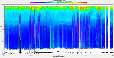
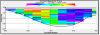
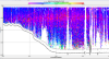
PHYSICAL - ADCP
Station 1 shows a
layer of increased backscatter at around 6-8m (Figure
16a), getting deeper near the end of the transect when it
descends to the seabed at around 10-15m. The typical
backscatter layer displays backscatter values of around
80-90 dBs. The velocity magnitude measurements show a
consistent speed from the surface down to the sea floor
of 0-0.2 m/s and the velocity direction is similar all
the way through the water column.
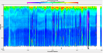
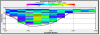
Interestingly,
station 2+3 both show evidence of double thermocline
formation (See Figure 15a). This
is reflected in increased backscatter occurring at
multiple deeper depths in the water column (see Figure
16b+16c), 80dB for both stations at the depths of the
possible second thermocline. Both station 3+4 showed
little variation in flow magnitude, however station 3
showed a shear forming between the surface layer and the
deeper layer caused by different directions of flow
(Figure 16d).
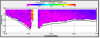
Station 4 showed a
weak thermocline, indicating a well mixed water column
(See Figure 15a). The ADCP was
not functioning correctly in this area, possibly due to
the strong swell we were experiencing, and therefore it
either did not record any data or the data was spurious
(e.g. showing extremely high values for current
velocity).
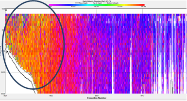
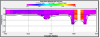
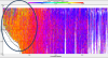
Station 5 was
recorded in a shallow cove (see Figure 12).
The headland of the cove has an influence on the flow
inside, causing turbulent eddies to form in the water
column (see Figure 16e, circled).
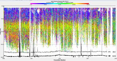
Station 6 shows
different directional flow at 15m, which corresponds to
a high backscatter reading (81 dB) also at 15m. The
magnitude of the flow is consistent from surface to deep
water.
Wind driven
currents at surface, could cause mixing and enhanced
primary production.
The backscatter
from the ADCP shows the possible formation of a deep
chlorophyll maximum at around 5-15 m, which would
correspond with the depth of the thermoclines of the
stations (Figure 15a). This
occurs when zooplankton graze on the abundant
phytoplankton which reside near the bottom of the thermocline where they have access to nutrients in the
deeper layer (Cullen J. J, 1982).
A few stations
(notably 2+3) both show the possible formation of a
double thermocline. This is mirrored in the chlorophyll
steps which are seen on the fluorometer reading (Figure
15d) at the bottom of both the thermoclines.
The shear created by the differing directions of water
flow will lead to mixing in the area, combining nutrient
rich water into the mixed surface layer (W.R. Young
et al, 1982) and allowing the deep chlorophyll
maximum to form. An example of this could be at station
6 where the surface water and the deeper water are
flowing in different directions, creating a shear and
increasing the backscatter at the same depth. This shear
could be formed by wind driven currents at the surface,
and this in turn would increase the mixing of nutrient
mixing water into the surface layer.
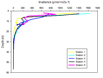
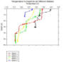
PHYSICAL - Light
The depth profile of
irradiance shows that light decreases exponentially with
depth at all stations, with rapid decrease in the
surface layers followed by slower decrease in deeper.
Station 1 shows the lowest values with the fastest
decrease, and station 3 the highest surface values.
Station 5 was a shallow inshore location, and shows
different results to other stations, as light can
penetrate to the seabed.
Station 1 (black rock)
is situated within the estuary, so the amount of
particulate organic matter POM will be higher here than
offshore stations. This POM will limit the amount of
light penetrating beyond the surface layers.
In
order to calculate the attenuation coefficient, the
natural log of the depth sensor readings ln(Ez) is
calculated and then plotted against depth, and from
this, the slope of the lines for each station can be
found. From the slopes, k (m-1) can be
calculated by 1/slope. The table shows the calculated
attenuation coefficient values, k.
|
Station |
Slope |
K (m-1) |
|
1 |
4.39 |
0.228 |
|
2 |
4.556 |
0.219 |
|
3 |
4.453 |
0.225 |
|
4 |
3.8641 |
0.259 |
|
5 |
6.79 |
0.147 |
A small attenuation coefficient suggests the water is
relatively transparent. Station 5 has the lowest k
value suggesting low levels of POM, whereas station 4
shows the highest coefficient suggesting there are
higher amounts of POM in this area. Looking at
fluorometer depth profile, there is a possible
chlorophyll maximum at around 12m, which could be an
explanation for the high attenuation coefficient.
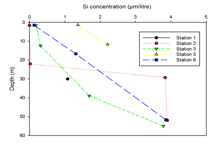
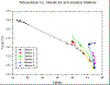
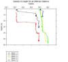
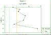
CHEMISTRY - Silicon
It is visible from the silicon vs. depth
figure, that the concentration of silicon increases with
depth. Values of <1
µmol/litre
in surface waters at stations 2, 3 and 6, and values of
around 4 µmol/litre
beyond 50m. station 5 shows higher surface values , this
station was inshore and shallow, which may explain the
difference in values.
Silicon is taken up by diatoms which use it to construct
their frustules. Diatoms require light for photosynthesis,
and therefore are generally found in the euphotic zone.
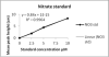
CHEMISTRY - Nitrate
Aim: To gain an insight into how
Nitrate changes with depth away from the coastal
environment.
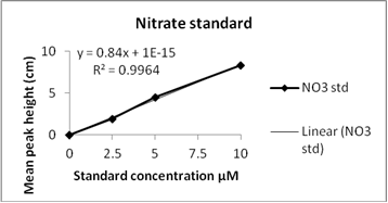
Method: water samples taken using
Niskin bottles around a CTD Rosette. 50ml water sample
filtered into a glass bottle for analysis using flow
injection method with a spectrometer measuring absorbance at
540nm. Standards of 0μM, 2.5μM, 5μM and 10μM Nitrate
concentrations were run and plotted against their mean peak
heights to gain a calibration equation to convert peak
heights of samples to concentrations.
Nitrate conc. = Peak height (cm) / 0.84
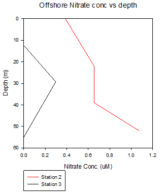
Station 2 shows an increase in Nitrate
concentration with depth in the surface 22m, steady
concentrations for the following 20m and a large increase in
Nitrate between 40 and 50m.
Station 3 describes Nitrate values
undetectable using our equipment in the surface 12m then an
increase in Nitrate from 0.296μM between 12 and 30m. Deeper
than 30m, Nitrate values are shown to drop off to
undetectable values by 55m.
Data for Stations 5 and 6 gave Nitrate
concentrations too low to detect while the lower detection
limit is bordered at 30m at Station 3 at .296μM with general
lower detection limits described as <.3μM, concentrations at
other depths at this Station, however are also too low to
detect.
An increase in detectable samples would
greatly improve this description of Nitrate behaviour at
these Stations. Station 2 provides the most clear and useful
results but does not give enough information to find, for
example the deep chlorophyll maximum. It does however
suggest highest phytoplankton photosynthesis rates at the
surface, shown by the lowest Nitrate concentration at the
Station. Photosynthesis rates are shown to slowly slow from
the surface to 22m where rates remain steady in the next 20m
of the water column. Below 40m, rates are seen to slow more
dramatically with a jump from 0.65μM to 1.1μM between 40m
and 52m.
Station 3 data displayed here is
unlikely to present an accurate interpretation of Nitrate
behaviour in the water column at this Station, the only
detectable value is just on the detection limit, as such
Nitrate concentrations at other depths may also be
exceptionally close to the detection limit but just off the
chart or may be considerably lower than the detection limit.
Equipment with a higher sensitivity
that could detect lower Nitrate values would hugely improve
this offshore analysis.
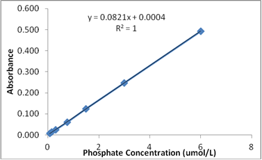
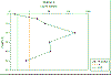
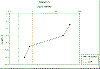
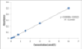
CHEMICAL - Phosphate
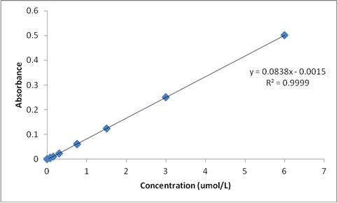
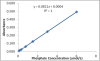
Concentration standards were mixed with
water to produce known concentrations, after measuring the
absorbance values of known concentrations, one can produce a
calibration line on a graph which can give the concentration
of a sample of a certain absorbance value (see figure 1).
This is done by rearranging the formula of the calibration
line (regression line) to solve for concentration:


Where, x = concentration of phosphate
in sample (umol/L), y = absorbance value of sample
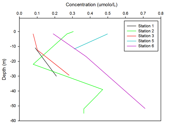
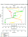
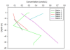
Phosphate samples were taken by the
bottles attached on to the CTD at different depths which
would give us it vertical distribution. The results seem to
suggest that concentration of phosphate increases with depth
generally. At station 4, the CTD was deployed; however no
samples were taken at the station. For station 1 and 5,
samples were only taken at 2 depths. Also, some samples had
replicas however; some of those values differed slightly
meaning that for those whose replica absorbance value differ
an average of the two was taken. At station 1, the
concentration increased from 0.089µmol/L at 11 metres to
0.209µmol/L at 30metres. At station 2, there is an initial
drop in concentration from the surface (0.304µmol/L) to
22metres (0.078µmol/L). Phosphate concentration increases
after that depth to 0.471µmol/L at 39 metres before dropping
at 55 metres to 0.364µmol/L. Concentrations also increase
with depth from 0.245µmol/L at 1.6 metres to 0.31µmol/L at
11.7 metre. Station 6 increases in concentration from
0.191µmol/L at 1.5m to 0.71µmol/L at 51.7m.
General trend of the figure shows that
chlorophyll increases with depth at all stations however,
stations 1, 3, 5 and 6 gives an incomplete picture of the
phosphate distribution across the water column at the
stations because only two or three depths were sampled.
Across over 60 metres of water in depth, this amount of
samples is not enough to give a high resolution picture.
At station 2, phosphate concentration
decreases from the surface to 22 metres. The CTD data shows
that roughly the same depth there is a chlorophyll maximum
(see figure for station 2 CTD), this indicates that primary
production is highest at that depth. This means that at that
depth phosphate concentration is low because it is used up
by the phytoplankton for growth. At this station, a tidal
front seems to have been observed; stratification of water
was also observed, the thermocline was also located at 17 to
28 metres which separates the nutrient depleted surface
waters from the nutrient rich waters at depth.
At station 3 although the resolution is
not very high, one can still observe the relationship
between chlorophyll concentrations and phosphate
concentrations. At station 3, phosphate minimum is at around
13 metres whilst the chlorophyll maximum occurs at 13.5
metres. A thermocline is also observed at those depths as
well meaning that there is also a front at this station,
however it is not as clear as at station 2 due to the fact
that not very many depths were sampled here.
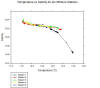
CHEMICAL - Oxygen
Generally oxygen saturation decreases with depth, over 100%
saturation in the surface waters at stations 2, 3 and 6, and
values below 90% beyond 50m. Station 2 shows a slight
increase with depth, followed by a dramatic decrease,
showing a possible chlorophyll maximum. All stations show
similar values, except station 5 (an inshore station) which
shows slightly lower saturation values.
CONCLUSION - Offshore
Six stations were sampled; however
weather constraints limited the distance offshore where
samples could be taken, so samples were taken closer to
the coast. Biological, chemical and physical parameters
were measured at each station.
A strong thermal stratification was
observed at the stations furthest from the shore. A
chlorophyll peak was found close or near to the
thermocline. Plankton was dominated by copepods and
copepod nauplii and Guinardia sritiata and a
possible tidal front was located between station 2 and
3. Low nitrate concentrations were found at the surface,
this correspond with higher levels of plankton, showing
nitrate is being consumed. Phosphate was found to
generally increase with depth as did silicon, but oxygen
decreased with depth.
The ADCP gave a valuable insight
into the physical and biological structure of the
offshore area which we studied. Backscatter graphs
consistently showed the formation of deep chlorophyll
maxima, largely around the areas where strong
thermoclines were forming. The velocity magnitude and
direction data also helped evaluate any possible shear
which was forming, possibly leading to mixing processes.
Sampling of more depths with more
precise equipment would have provided higher resolution
data, so conclusions could have been more solid.
|
|
Date |
30/06/2012 |
|
Location |
Falmouth Offshore |
|
Wind |
F5 SW |
|
Tide |
1350 |
|
Weather |
Overcast |
|
Sea State |
Rough |

Figure 12 - Transect
map for the Offshore route
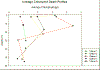
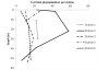
Figure 13 -
Average chlorophyll values plotted against depth with
increasing offshore distance
(a)
  (b)
(b)
(c)
(d)
  (e)
(e)
(f)
  (g)
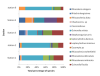
(g) Figure
14a-g: (a) and (b) Total percentage of diatoms found for all
five offshore stations; (c)
Percentage of total
phytoplankton for each station against depth;
(d)
percentage of zooplankton
found for all 5 stations; (e) Zooplankton for each station
at given depths (bottle 21 is station 1, bottle 22 is
station 2, bottle 23 is station 3, bottle 24 is station 5
and bottle 25 is station 6); (f)
Guinardia striata
(Coale, 2007); (g) Copepod (Kils, 2002)
(a)
  (b)
(b)
(c)
  (d)
(d)
(e)
  (f)
(f)
(g)
  (h)
(h)
(i)
Figure
15a-i: (a) Temperature at all Offshore stations; (b)
Salinity at all Offshore stations; (c) Temperature-salinity
plots for all offshore stations; (d) Fluorescence at
all Offshore stations; (e) All parameters at Station 1; (f)
All parameters at Station 2; (g) All parameters at Station
3; (h) All parameters at Station 4; (i) All parameters at
Station 5
(a)
  (b)
(b)
(c)
  (d)
(d)
(e)
  (f)
(f)
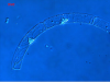
Figure 16a-f: (a)
Backscatter contour for Station 1; (b) Backscatter contour
for Station 2; (c) Backscatter contour for Station 3; (d)
Flow direction data for Station 3; (e) Velocity
direction data for Station 4; (f) Velocity direction data
for Station 5
(a)
  (b)
(b)
(c)
(d)
  (e)
(e)
Figure 17a-e: (a)
Richardson Number for Station 1; (b) Station 2; (c) Station
3; (d) Station 4; (e) Station 5
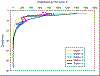
Figure
25. Depth profile showing how the irradiance varies with
depth at all offshore stations, except station 6 due to
corrupted CTD files.
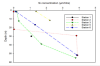
Figure 17. Silicon concentration as
depth increases for all stations offshore, except station 4
where no bottles were fired.
(a)
(b)
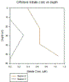
Figure 18a-b:
(a) Nitrate standard; (b)
Offshore nitrate concentrations with depth
(a)
  (b)
(b)
Figure 19a-b: (a)
Phosphate standards; (b) Phosphate concentrations with depth
at each station
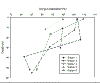
Figure 20. Oxygen saturation depth
profile at all stations offshore, except 4, where no bottles
were fired.
|
|

|
|
Pontoon
|
Introduction
A YSI
6600-D V2 multiprobe, a Li-Cor Li-1400 datalogger and
Valeport current meter were used to take quarter hourly
measurements over a 3.75 hour period of an ebbing tide
from a chain ferry pontoon on a shallow 5-6m reach of
the upper Fal river which had experienced rainfall
overnight.
Aim:
Collect a time series of various seawater parameters
over the tidal cycle.
Results & Discussion
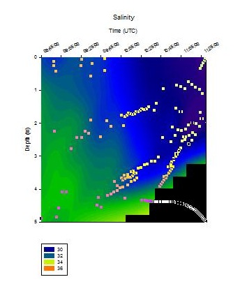
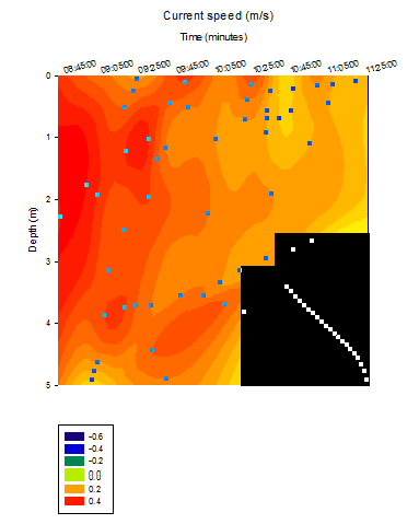
The
water level shoaled from 5 m to 3 m with the ebbing tide
as a function of time and black blocks in Figures
21a-21i indicate seabed when incomplete data sets were
taken as a result of this. Salinity decreased from 34
to 30 at the surface as the tide ebbed with lower
salinity, less dense freshwater overlying tidally driven
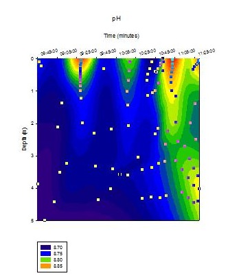
seawater (Figure 21a). Initially surface pH became more
alkaline as the tide ebbed, this extended throughout the
water column by the end of the survey when the water
depth had decreased from 5 to 3m (Figure 21b). The Fal
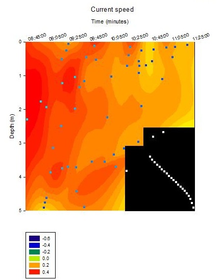
river current speed at the pontoon was measured as
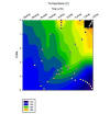
0.2-0.4 m/s (Figure 21c). Temperature at 14 o
C was lowest at depth and increased from the surface
throughout the water column with shoaling of the
retreating tide and increased seasonally warmed riverine
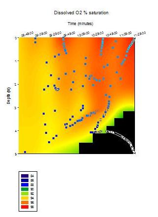
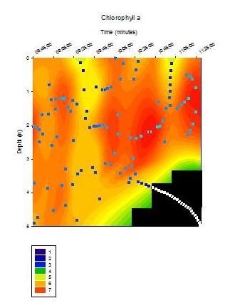
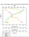
input (Figure 21e).The chlorophyll
α
concentration was highest at 7 µg/L at mid depths of
1.5-3 m and 6 ug/L at the surface when the water depth
was 5 m decreasing to 5 µg/L for two quarter-hour
periods possibly related to an intermittent increase in
sunlight or dispersal related to a onside docking ferry.
As the water level decreased to 3m the peak moved
towards the surface (Figure 21e). Initial dissolved
oxygen levels were 96% at the water surface with lower
levels of 92% at 5m depth; the water column homogenised
at its 3 m minimum and reached a saturation peak of 98%
within the surface 0.5 – 2 m. The latter two parameters
are proxies of phytoplankton activity and suggest
possible UV shading in the surface above 0.5 m.
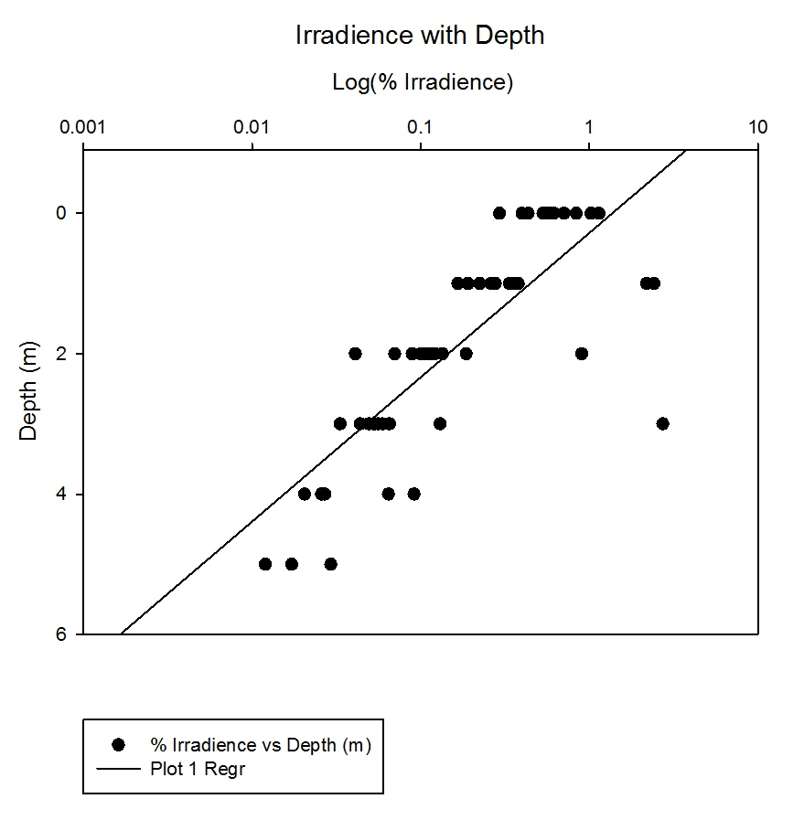
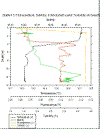
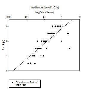
Depth
profile of ln (irradiance
µmol/m2/s)
shows an exponential decrease with depth, the
compensation depth above which phytoplankton
photosynthesis is 10 µmol/m2/s (Miller,
2001). This is due to the attenuation of light as it
moves through the water column, it is scattered and
absorbed by various particles. A few points display
higher than expected levels, these can be accepted as
anomalies.
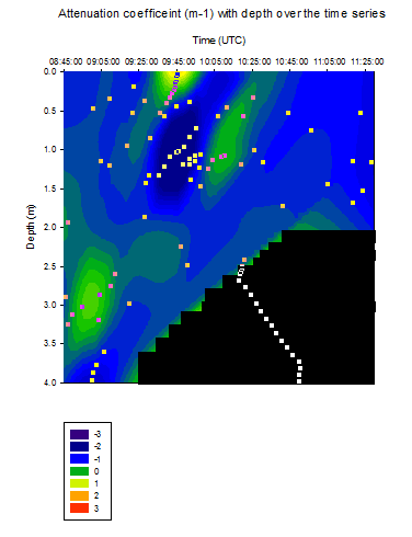
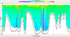
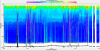
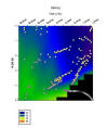
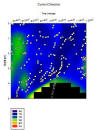
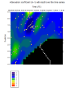
Figure 6, the
attenuation coefficient plot, shows generally stable
light penetration throughout the time series. The area
of higher k values in the surface waters at 09.45UTC
could represent an area of plankton dominance. Under
this area is an area of lower k values, where the
plankton has blocked the light from penetrating to
deeper water. The area of high k values at around 3m at
the beginning of the time series could represent
sediment disturbance.
Pontoon
conclusion
The pontoon station was used to
collect chemical and physical data from one station on
an ebbing tide.
Surface salinity decreased as the
tide was ebbing and its influence was reduced and pH
became more alkaline as surface river flux increased.
Initially irradiance decreased with depth due to light
attenuation but as the depth shoaled as a function of
time the water column homogenised and the compensation
depth was raised increasing the euphotic zone and
phytoplankton proxies increased in response to this.
|
|
Date |
04/07/2012 |
|
Location |
Fal River |
|
Wind |
F2 S |
|
Tide |
HT 0619 |
|
Weather |
Sunny spells |
|
Sea State |
Calm |
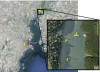
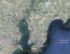
Figure 26.
Google earth image of Pontoon site.
(a)
  (b)
(b)
(c)
  (d)
(d)
(e)
  (f)
(f)
(g)
  (h)
(h)
 (i) (i)
Figure
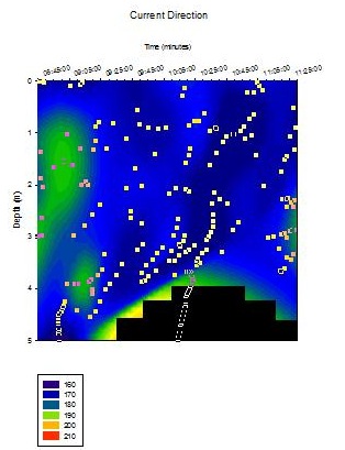
21a-h: (a) YSI salinity profile; (b) YSI pH profile; (c)
Irradiance with Depth; (d) YSI oxygen profile; (e)
Directional flow profile; (f) Current velocity profile; (g)
YSI chlorophyll a profile; (h) YSI temperature profile
|
|
|
|
Geophysics
- View the e-poster
here |
|
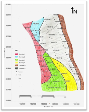
A Geophysical
survey was conducted along the coastline off Castle Head
at the Western edge of the Fal estuary mouth involving
Side Scan sonar (4 transects), grabs (3 along three of
our 4 transects due to worries about proximity to
shoreline danger to the vessel) and underwater video
footage of the bed (across 2 of our transects) in order
to establish biota and bed types across the survey area
allowing the creation of habitat maps combining physical
and biological properties. This habitat mapping exercise
is aimed at likely implications on maerl and other life
forms that may result from the planned dredging of the
channel in the estuary at the proposed sites.
Maerl is an
extremely slow growing (1mm/year) coralline algae,
creating its own calcium carbonate structure upon which
it can grow. It is only in recent years that dredging of
maerl for use as fertiliser in the agricultural world
was banned due to reports stating that maerl was too
slow growing to be considered a sustainable resource
while the benefits of living and dead maerl in providing
shelter for juvenile species was realised resulting in
maerl beds in the Fal estuary being given a protected
status. Now there are exceptionally strict limitations
on any disturbance of maerl beds across the estuary.
Disturbance of sediment beds and habitat dynamics due to
the proposed dredging the Fal channel and the resulting
settlement of fine sediment are a worry.
TRANSECTS
Subsurface Duel Frequency Analogue
Side Scan Sonar at a frequency of 410 kHz (high
resolution images) was used with a swath range of 200m.
Transects were 100m apart and alongside one another so
overlapped allowing full analysis of surveyed area. The
tow fish was towed with a layback of 4m both vertically
and horizontally, corrections were not made due to the
small scale of these errors.
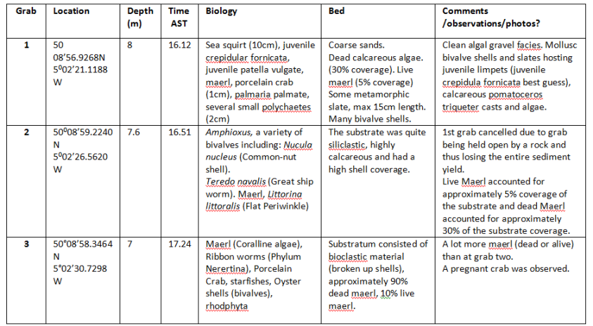
GRABS
3
grab samples along each transect line deemed deep enough
to safely conduct the grab. Using a Van Veen grab
allowed ground truthing comparing and confirming side
scan data. Van Veen grab lowered to sea floor on a
marine-grade stainless steel hydrographic line. Grabs
then sieved through 1cm and 1mm sieves to analyse
sediment sizes. Photographic evidence taken for later
species identification.
VIDEO ANALYSIS
Video analysis of the bed over the
area surveyed allows further ground proofing, helping to
confirm the sidescan analysis as well as providing real
images of the structure of the bed type and biota in
their natural state. This is useful in exploring habitat
dynamics. Camera was lowered from starboard side of the
boat to 7m, just above the bottom. Boat drifted during
video.
Video footage was available for
only one expected boundary crossing upon analysis of the
sidescan sonar, this boundary was evident with more
coarse grained, maerl rich gravels covered by bivalve
mollusc shells giving way to finer grained sediment
between boundaries 6 and 5. Numerous starfish were seen
along the video transect, small fish were seen to swim
away from the camera preventing identification.
High resolution side scan sonar
with relatively few artifacts allowed a clear
representation of the sea bed in the survey area. Ground
proofing through grabs and video footage has confirmed
our analysis of a small area of the survey area, on
reflection grabs could have been taken diagonally across
the whole area in order to avoid ground proofing in the
same boundary zone and increased video footage more
fully describing the survey area would have provided
tools for greater accuracy in our analysis of the side
scan data.
|
|
Date |
26/06/2012 |
|
Location |
Fal Estuary |
|
Wind |
F2 SW |
|
Tide |
0922 |
|
Weather |
Overcast |
|
Sea State |
Calm |
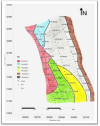
Figure
21: Habitat
map
of transects and interpretation of side scan sonar showing
boundary layers of bed forms, grab sites and path of video.
(a)
  (b)
(b)
(c)
  (d)
(d)
Figure22a-d: Tables of relevant coordinates and times for
each individual grab made for the geophysical survey

Figure
23: Table of findings from the grabs

Figure
24: Table of coordinates and times for the video transect |
|

|
|
Conclusions
|
|
Aim: To gain
an understanding of the physical, chemical and biological
processes in the Fal Estuary and the surrounding coastal
waters.
A number of processes were used to
gather information about the physical, biological and
chemical processes within the Fal estuary and the
surrounding coastal waters, information was collected in the
field and studied in the laboratory.
The estuary samples gave a more
horizontal profile as the depth was too shallow in parts to
get a detailed vertical profile. The nutrients generally
decreased with increasing salinity down the estuary whilst
turbidity would increase due to deposition. The offshore
study gave a more vertical profile as sampling occurred at
deeper depths. A strong thermal stratification was found
offshore. Low nitrate was found at the surface, phosphate
increased with depth. We were also able to use an ADCP to
analyse both physical and biological properties of the water
column in the estuary and offshore. With this data we were
able to determine a chlorophyll maxima and mixing profiles.
The pontoon practical gained an insight into physical and
chemical properties of an estuary as the tide was ebbing,
giving a vertical profile at 1 station over time.
Zooplankton in both the estuary and
offshore were dominated by copepod and copepod nauplii and
the phytoplankton was dominated by Guinardia striata.
There
were some constraints when conducting practical work such as
weather, equipment and depth of water columns.
|
|
|
|
Appendix
|
Equipment and methods sections were
included to avoid repetition occurring in our write ups.
As the methods and equipment used in certain
investigations were similar (e.g. chemical analysis for
offshore and estuarine studies) we felt it would be
appropriate to give a general overview of our processes
to avoid repeating ourselves.
We would like to thank the boat
crews, academic staff and demonstrators for all the help
and advice given over the course of our survey. Their
expertise was vital in the completion of our survey.
The view and opinions expressed in
this report are that of our own, and do not necessarily
reflect the views of the University of Southampton.
|
|

|
|
References
|
|
1997 Phosphorus Cycling in the
Estuarine Environment [http://www.co.bell.tx.us/bellnet/bellnetweb/web/phosphor.htm,
Accessed: 05/07/2012]
Bryan, G.
W. and Gibbs, P.E. 1983. Heavy metals in the Fal estuary,
Cornwall: A study of long term contamination by mining waste
and its effects on estuarine organisms. Occasional
Publications, Marine Biological Association of the United
Kingdom, 2: 112.
Campbell, A.C. Nicholls, J 1986 The Hamlyn
Guide to Seashores and Shallow Seas of Britain And Europe.
Hamlyn Publishing Group Ltd
Chen. C.T.A. 1998. Nutrient cycling in the
oceans. Oceanography. 1.
Cho, J.H. 2007. Effects of
prevailing wind on turbidity of a shallow estuary.
International Journal of Environmental Research and Public
Health, 4 (2): 185 – 192.
Coale, S. 2007. Guinardia
striata: Diatom. [http://cimt.ucsc.edu/hab%20id/phytolist_diatoms/18guinardia.html,
Accessed 04/07/2012]
Cullen J.J.
1982. The
deep chlorophyll maximum: Comparing vertical profiles of
chlorophyll a, pg 799.
Franks, P.J.S 1992. Plankton
Blooms at Fronts: Patterns, Scales and Physical Forcing
Mechanisms. Reviews in Aquatic Sciences. 62(2),121-137.
Grasshoff K. 1983. Determination of oxygen,
Methods of Seawater Analysis. 61-72 (Eds)
Huisman, J.,Oostveen, P.V., Weissing, F.J.
1999. Critical depth and crtical turbulence: two different
mechanisms for the development of phytoplankton blooms.
Limology and oceanography. 44, 7,
1781-1787.
Johnson, M.P., Hartnett, M.,
Collier, L.M. and Costello, M.J. 2002. Identifying “hot
spots” of biological and anthropogenic activity in two Irish
estuaries using means and frequencies. Hydrobiologia,
164: 111 – 123.
Johnson K. and R.L. Petty 1983. Determination
of nitrate and nitrite in seawater by flow injection
analysis, Limnology and Oceanography, 28,
1260-1266
Jorgensen, B.B. and Richardson, K. 1996.
Eutrophication in coastal Marine Ecosystem. Coastal and
Estuarine studies, 52.
Kils, U. 2002. Introduction
to the Copepoda. [http://www.ucmp.berkeley.edu/arthropoda/crustacea/maxillopoda/copepoda.html,
Accessed 04/07/2012]
Knauss, J. 1997. Introduction to Physical Oceanography, Second
Edition, Waveland Press
Kraberg, A., Baumann, M. and
Durselen, C.D. 2010. Coastal Phytoplankton. Photo guide for
Northern European Seas. Alfred Wegener Institute for Polar
and Marine Research. Munchen. Germany
Langston, W.J. Chesman, B.S. Burt, G.R. Hawkins, S.J.
Readman, J. Worsford, P. 2003. "The Fal and Helford cSAC".
Marine Biological Assoication Occasional Publication
No. 8
Langston W,
Chesman B, Burt G, Taylor M, Covey R, Cunningham N, Jonas P,
Hawkins S. 2006. 'Characterisation of the European Marine
Sites in South West England: the Fal and Helford candidate
Special Area of Conservation (cSAC)'. Marine Biodiversity.
Volume 183, 321-333.
Larink, O. and Westheide, W.
2006. Coastal Plankton. Photo guide for the European Seas.
Alfred Wegener Institute for Polar and Marine Research.
Munchen. Germany
Li-Cor light
meters. 2012. Available at
www.licor.com/env/products/light.htm.
(Accessed 5 July 2012).
Liu Q.,
Y. Jia, P. Liu, Q. Wang, P.C. Chu 2001. Seasonal and
Intraseasonal Thermocline Variability in the Central China
Sea, Geophys. Res. Lett. 28, 23,
4467-4470.
Nejstgaard, J.C et al. 2001.
Zooplankton growth, diet and reproductive success compared
in simultaneous diatom- and flagellate microzooplankton-
dominated plankton blooms. Marine Ecology Progress Series.
221 (3), 77-91.
Parsons TR,
Lalli C. 1984. A manual of chemical and biological
methods for seawater analysis. 101-112. Pergamon
Press, Oxford.
Pingree.
R.D, Holligan. P.M., Mardell. G.T. 1978. The effects of
vertical stability on phytoplankton distributions in the
summer on the northwest European Shelf. Deep Sea Research.
25. 11. 1011-1016
Smyth T.J., J.R. Fishwick, L.
Al-Moosawi, D.G. Cummings, C. Harris, V. Kitidis, A. Rees,
V. Martinez-Vicente and E.M.S. Woodward 2009. A broad spatio-temporal
view of the Western English Channel observatory, Journal
of Plankton Research, 32, 5,
585-601.
Somerfield, P. J. Gee, J. M. Warwick R. M. 1994. Soft
sediment meiofaunal community structure in relation to a
long-term heavy metal gradient in the Fal estuary system.
Marine Ecology Progress Series 108. 79-88
Southward A.J., Langmead O., Hardman-Mountford
N.J., Aiken J., Boalch G.T., Dando P.R., Genner M.J., Joint
I., Kendall M.A., Halliday N.C., Harris R.P., Leaper R.,
Mieszkowska N., Pingree R.D., Richardson A.J., Sims D.W.,
Smith T., Walne A.W., Hawkins S.J. 2005. Long-Term
Oceanographic and Ecological Research in the Western English
Channel’
Advances in Marine Biology,
47
Valeport
current meters and open channel meters. 2012. Available at:
www.valeport.co.uk/products/currentmeters.aspx.
(Accessed 5 July 2012).
Van Haren
H. 2000. Properties of vertical current shear across
stratification in the North Sea, Journal of Marine
Research. 58, 3, 465-491 (27). Pub:
Sears Foundation of Marine Research.
Violette, P. 1995. Seasonal
and Interannual variability of the Western Mediterranean.
Coastal and Estuarine Studies.
Welschmeyer
N.A. 1994. Fluorometric analysis of chlorophyll a in the
presence of chlorophyll b and pheopigments.
Widdicombe, C.E., Eloire, D.,
Harbour, D., Harris, R.E. and Somerfiled, P.J. 2010.
Long-term phytoplankton community dynamics in the Western
English Channel. Journal of phytoplankton research.
32. 5. 643-655
Wooldridge
T. and T. Erasmus 1980. Utilization of tidal currents by
estuarine zooplankton, Estuarine and Coastal Marine
Science, 11, 107-114
Young P.R.,
P.B. Rhines and C.R. Garrett 1982, Shear flow dispersion,
internal waves and horizontal mixing in the ocean, pg
515. |
|
|