

 The Fal Estuary is located on the south coast of Cornwall in the UK,
where it extends 18km inland from its entrance at Pendennis Point and
St. Anthony’s Head to its tidal limit at Tresillian.
The Fal Estuary is located on the south coast of Cornwall in the UK,
where it extends 18km inland from its entrance at Pendennis Point and
St. Anthony’s Head to its tidal limit at Tresillian.
It is the world’s third largest natural harbour with a total shoreline length of 127km, making it extremely important in terms of tourism, trade and conservation.
The Fal estuary is a classic ria or drowned river valley, formed at the end of the last period of glaciation due to sea level rise. The Estuary can be divided into two main areas; The inner tidal area which is compromised of its many tributaries including the River Truro, River Fal, River Penryn and 28 tidal creeks and the outer tidal basin known as the Carrick Roads. The Carrick roads makes up 80% of the body of the estuary with a maximum depth of 35m, it is the third deepest harbor in the world (Langston, et al., 2006)
The estuary shows macrotidal characteristics at the mouth of the estuary but develops mesotidal features further upstream. Strong tidal mixing within the estuary with currents of up to 2 knots makes the influence of freshwater inputs negligible. The catchment and sediments of the Fal Estuary reflects its underlying geology, with Carnmellis granite and surrounding metamorphic rocks to the west, while china clay and mining wastes have been added to the sediments particularly from the St. Austell area and the Carnon River Valley respectively. Although little of the mining industry is still active today to contribute to the pollution in the region, the residual drainage from abandoned mines continue to affect the sediment geochemistry when the contaminated sediments are being distributed around the estuary.
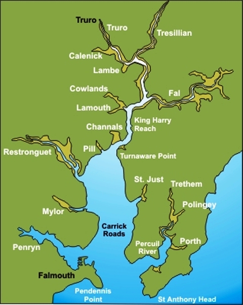
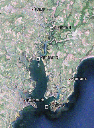
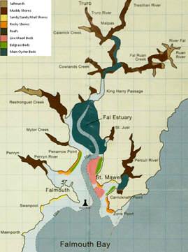
Figure 1 (right) is a map of the area directly surrounding Carrick Roads and the Fal Estuary.
The estuary is classified as a Special Area of Conservation (SAC) under the Habitat’s Directive due to the number of important habitats that can be found in the area, including maerl beds at St. Mawes Bank and seagrass beds, both providing vital habitats for associated marine species (Langston, et al., 2006). Other habitats of interest include saltmarshes that are important for bird populations and mussel beds.
Between the 27th of June and the 6th of July our group conducted surveys in the estuary and offshore locations and also laboratory tests with the aim to develop an understanding of the biological, chemical, physical and geological processes that occur in the Fal Estuary and surrounding coastal waters.
The Team (back to top of Introduction/webpage)
Chloe Whitfield
Graeme Loveday
Harry Levick
James Ziemann
Matthew Carson
Ollie Parker
Rebekah Susserott
Richard Hofman
Sophia Roach
Offshore Boatwork - Materials and Methods, Results (back to top of webpage)
The aim of the offshore fieldwork was to answer the question of what effects vertical mixing processes in the coastal waters off Falmouth have directly or indirectly on the structure and properties of the planktonic communities. In addition, the physical, chemical and biological processes that occur spatially within the water column from the mouth of the Fal Estuary and the waters to the east of the estuary were also investigated.
The waters in the Western English Channel are usually thermally stratified during the summer months. The degree and extent of the stratification is determined largely by the water depth and the tidal strength. The structure of the water column is also affected by the input of freshwater, wind strength and other climatic factors.
The physical and chemical properties of the surface layer of the water column are heavily influenced by vertical mixing, which controls the abundance and distribution of planktonic communities as a result (Kiorboe, 1993). As such, locating and understanding frontal systems, which occur as a result of interaction between stratified and well mixed water masses, is crucial to our understanding of planktonic communities in coastal seas. Therefore, fronts can be said to form at boundaries of both temperature and salinity, which is greatly influenced by the topography and tidal cycle of the area, especially in coastal regions, affecting the level of mixing within the system (Fogg, et al., 1985).
As the area surrounding frontal regions are affected by stratified and mixed bodies of water, great variations in physical characteristics, such as temperature, salinity and nutrient concentration, occur.
Nutrient concentration is high in the well mixed water mass, with the surface waters replenished by the cold, nutrient rich bottom waters. In stratified waters, like those seen in the summer months, nutrient depletion is a common characteristic. Therefore, a key issue in this investigation is the rate at which nutrients can be mixed upwards across the thermocline. By understanding this process, variations in biological productivity at this time of the year can be explained, and our understanding of the physical, chemical and biological aspects surrounding frontal regions and adjacent waters can be furthered.
Materials and Methods (back to top of Offshore Boatwork/webpage)
![]() On board the RV Callista an approximate transect was
laid out in a South Easterly direction from the Fal Estuary with 4
Stations at which data sets were going to be collected. Throughout the
trip the Acoustic Doppler Current Profiler (ADCP) was running, being
restarted between each of the stations for ease of data interpretation
at a later date. This was primarily used to find areas of high-density
backscatter, which is indicative of plankton blooms.
On board the RV Callista an approximate transect was
laid out in a South Easterly direction from the Fal Estuary with 4
Stations at which data sets were going to be collected. Throughout the
trip the Acoustic Doppler Current Profiler (ADCP) was running, being
restarted between each of the stations for ease of data interpretation
at a later date. This was primarily used to find areas of high-density
backscatter, which is indicative of plankton blooms.
At each station, measurements were taken throughout the water column using a CTD rosette. The CTD was equipped with several different instruments in order to achieve this, a fluorometer to measure chlorophyll concentrations, a TS probe to measure depth and Salinity, an Irradiance meter to measure light penetration, and a transmissometer to measure turbidity. Niskin bottles attached to the CTD rosette were used to collect discrete water samples from the water column and could be remotely fired at the desired position in the water column (Bottom Depth, Chlorophyll Maximum, and Surface). To give another measure of light attenuation through the water column, a Secchi disk was lowered into the water column at each station.
Figure 2 (right) shows our survey line superimposed onto a map from google earth.
Once water samples were collected from the Niskin bottles, they were treated in preparation for lab analysis. To test for phosphate and nitrate 50ml of the sample was filtered into a glass bottle and stored. For silicate, 50ml of the sample was filtered and stored in a plastic bottle. The two filters used were placed in acetone and stored so that chlorophyll content could be measured in the lab. To test for dissolved oxygen, 1ml of manganese sulphate was added to 50ml of the water sample, followed by 1ml of potassium iodide. In order to preserve phytoplankton for lab analysis, lugols iodide was added to 100ml of the water sample. These protocols were carried out for each of the water samples collected at each depth.
Also at each station, a 200μm mesh, 62cm diameter zooplankton net was deployed and dragged up through the water column from a depth determined from the CTD data and then closed at the desired depth. The sample of zooplankton collected was then treated with a 10% formaldehyde solution in order to kill all living organisms and cease any biological and chemical processes occurring in the sample.
CTD rosette
The CTD (conductivity, temperature, depth sensor) is an instrument package that houses instruments for measurements of salinity, temperature and depth at which it is sampling. It can also house a variety of other sensors and equipment such as Niskin water bottles to take water samples at different depths. The CTD that was used for our offshore fieldwork supported a six Niskin bottle rosette and various other sensors including a fluorometer, transmissometer, platinum resistance thermometer, sensor for conductivity and a light sensor. Data from each depth is sent back to the vessel electronically via a conducting cable that is attached to the top of the CTD.
Niskin bottles
A Niskin bottle is a plastic bottle that has a spring loaded mechanism to close both ends of the bottle at the required depth, there by obtaining a sample of the water at that depth. The bottles can be shut electronically when attached to the CTD frame via a conducting cable connected to the vessel, or can be shut by dropping a messenger (weight) along hydroline onto the spring when being used individually like when sampling on the Pontoon. These bottles, that can hold up to 6 litres of water, allow water samples to be taken from different depths when sampling along a vertical profile.
Transmissometer
A transmissometer measures the attenuation of light in the water column by shining a light from one end of the instrument to the other at a set distance, with the amount of light reaching the receiving end from the output end varying between conditions underwater. The attenuation coefficient is then calculated from how much energy reaches the receiver. In turbid waters, the amount of energy that reaches the receiver will be smaller, while the opposite is true for clear waters. This instrument was attached to the CTD rosette for offshore and estuary fieldwork.
Fluorometer
A fluorometer measures the fluorescence in the water column by emitting a blue excitation beam which causes the chlorophyll in the phytoplankton in the water column to fluoresce. The instrument then gives a value for fluorescence which can be converted to chlorophyll concentration using an equation. The fluorometer was attached to the CTD rosette frame for both offshore and estuary fieldwork, allowing a vertical profile of chlorophyll to be obtained.
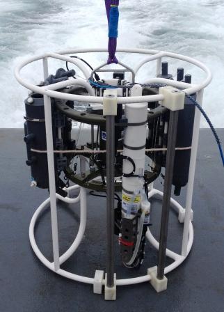
Figure 3 (above) Shows a CTD rosette system fitted with censors to measure fluorescence, turbidity, salinity, temperature and PAR. The CTD rosette was also equipped with 6, 1 litre Niskin bottles which could be fired remotely to take discrete water samples.
ADCP
Callista's onboard ADCP (Acoustic Doppler Current Profiler), housed in a moon pool on the hull, was used to quantify water velocities, magnetic shear, backscatter and current direction at different depths in the water column. The ADCP has a transducer, which sends out acoustic pulses and a receiver, which receives returning pulses. Through the use of three beams (with a fourth in reserve in case of failure) and the principle of the Doppler Shift, the mentioned parameters can all be measured accurately.
Secchi disk
A Secchi Disk is a weighted black and white plate that estimates the penetration of light in the water column. By measuring the depth to which one loses sight of the Secchi Disk, the light attenuation coefficient and an estimate of the euphotic zone (three times the Secchi Disk depth) can be calculated. The use of the Secchi Disk is very subjective, as the judgement of when the disk can no longer be seen varies between the people using it. Factors such as amount of suspended particles, light incident angle, phytoplankton blooms and turbidity can increase the light attenuation. The disk was deployed during fieldwork offshore and on the estuary.
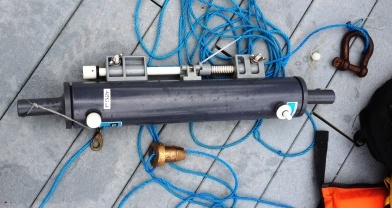
Plankton net
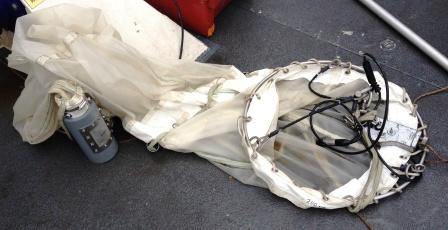
A plankton net is a net, funnel structure that is trawled through the water column for the collection of planktonic organisms. The size and type of the organism collected can be dictated by the mesh size. During offshore fieldwork, a ring plankton net of 0.6m in diameter with a mesh size of 200 microns was used to collect plankton. A collection bottle at the end of the net allowed the collection of planktonic organisms larger than the mesh size of the net.
Figure 4 (right) is the phytoplankton net that was used on the R.V. Callista.
Results - Physical Results, Chemical Results, Biological Results (back to top of Offshore Boatwork/webpage)
Physical results (back to top of Results/webpage)
CTD Casts
At station 1 the water column was stratified with, warmer, fresher waters towards the surface gradually increasing in salinity and decreasing in temperature towards the seafloor.
The water column at Station 2 had a stratified layer (~top 12m) which was fresher and warmer than the homogeneous deep layer that extended from 20m to the seafloor.
At station 3 clear thermo and haloclines were visible at ~25m with a fairly homogenous warmer fresher layer sat above a cooler more saline layer below.
Station 4 shows the strongest of the observable thermoclines with a temperature drop of ~2 degrees C over a distance of ~5m and a salinity drop of 0.2 PSU which is double the drop seen at Station 3 (the next strongest gradient).
The general trend observable as water depth and distance from shore increased was a deepening of the thermocline and halocline and increasing homogeneity of surface water layers and deeper waters.
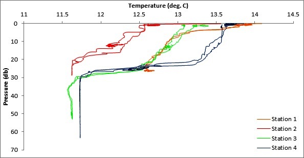
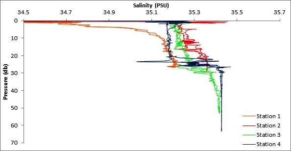
Figure 5 (above top) and Figure 6 (above bottom) are a graphs generated from CTD
data to explore the variability in temperature and salinity with depth for all 4 offshore stations.
Richardson's Numbers from ADCP results
Irradiance
Irradiance data collected during the CTD profiling showed similarly shaped depth profiles of attenuation for each station (Figure 6). Light intensity attenuates as it passes through the water column due to scattering and absorbance from suspended particles. The Euphotic zone, an area in the top layer of the ocean where light levels are sufficient to support photosynthesis, extends to a depth where the photosynthetically active radiation (PAR) is equal to 1% of its surface value. This depth is largely influenced by the turbidity of the water column.
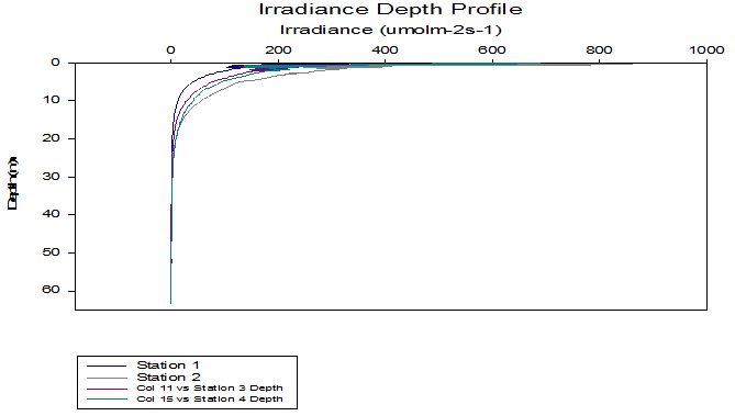
Figure 6 (above) shows light attenuation at each of the Offshore stations.
Secchi disk depth measurements, taken at each of the stations, were used to estimate the depth of the euphotic zone. Although such measurements may give a good indication of depth, horizontal movement of the disk in the current and inconsistency in human judgement may skew results making them inaccurate. Using the equation Ez = Eo e-kz and Irradiance data collected by CTD the attenuation coefficient (k) and 1% light depth for each station were calculated. These values, shown in table 1, were considered to be more accurate and a better representation of the true depth of the euphotic zone at each station.
|
|
Secchi Depth (m) |
Euphotic Depth Estimation (m) |
k - Attenuation Coefficient Secchi (m-1) |
k - Attenuation Coefficient CTD (m-1) |
1% Light Depth (m) |
|
Station 1 |
4.5 |
13.5 |
0.32 |
0.23 |
20.0 |
|
Station 2 |
6.5 |
19.5 |
0.22 |
0.20 |
23.3 |
|
Station 3 |
5.0 |
15.0 |
0.29 |
0.21 |
22.0 |
|
Station 4 |
7.0 |
21.0 |
0.21 |
0.18 |
25.7 |
Table 1 is a comparison of attenuation coefficients calculated by secchi disk measurements and PAR readings from the CTD.
Figure 2 is a graph of the respective depths for the bottom of the euphotic zone. It is common for the Secchi disk measurments to produce an over-estimate of the depth of the euphotic zone, however in this case the depths are shallower then the calculated 1% depth. It is likely that the sea roughness causing the secchi disk to travel under the boat and making it harder to detect played a part in this. Depite this, the general pattern of change of depth with station appears similar.
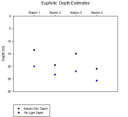
Figure 7 (above) shows the difference between calculated attenuation coefficients (k) of PAR from the CTD measurements and from the secchi depth.
Station 1, located at Blackrock near the mouth of the estuary showed the shallowest euphotic zone due to its close proximity to the estuary and subsequent high load of suspended sediment in the water column. As the stations progress along the transect into the open ocean it is seen that less light is attenuated per meter and the euphotic zone deepens. As depth of the water column increases decreased effect of wave action on the seafloor and a greater distance from the seabed reduces the amount of suspended sediment in the upper water column, reducing turbidity. Station 3 shows a decrease in euphotic depth, this deviation from the trend correlates with high levels of phytoplankton in the surface waters which would have caused increased turbidity.
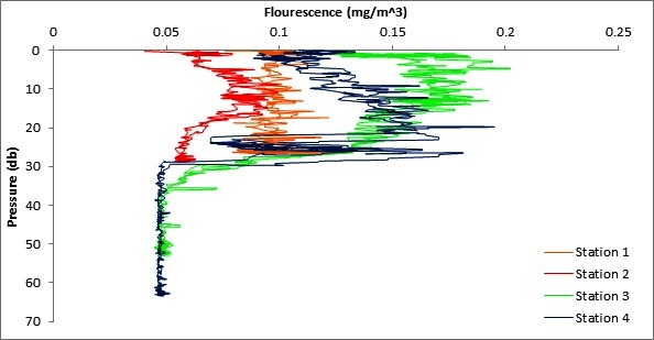
Figure 8 is a graph generated from CTD fluorescence data to explore how chlorophyll maximum depth changes as distance from shore increases.
The fluorescence values for station 1 show little variability from the surface all the way down to the seafloor.
Station 2 shows a peak in fluorescence values at ~12m after which there is a steady decrease in fluorescence readings.
At Station 3 the fluorescence values are high in the upper waters and reach a peak at around 15m and then drop off steadily until 30m at which point there is a sharp decrease to almost 0.
The fluorescence values at Station 4 increase steadily with depth until reaching a peak at around 28m (the deepest of the 4 Stations) at which point values decrease very sharply decreases to almost 0 at 30m.
NB: The CTD recorded PAR which includes only a specific range of wavelengths of light and this will be one reason that the Secchi depth is so different. Also the Secchi readings were taken with significant swell and some tidal action with the rope being far from vertical which may have additionally increased the difference between the two values.
Chemical Results (back to top of Results/webpage)
Figure 9: Scatter Graph of the nutrient profiles of station 1
Figure X (above) shows that as we moved down the water column from the surface to 26 metres the temperature dropped, by 1.29 °C and the salinity increased by 0.59. The phosphate concentration was higher at depth, increasing from 0.1655 to 0.2748 ug/L as was the concentration of dissolved oxygen (230.9640 to 292.5255 umol/L). However the silicate concentration dropped slightly with depth, decreasing from 2.6803 to 2.6122 ug/L.
Figure 10: Scatter Graph of the nutrient profiles of Station 2
Figure X (above) shows that as we moved down the water column from 12 meters to 28 metres the temperature dropped, by 0.52°C and the salinity increased by 0.8. The phosphate concentration was higher at depth, increasing from 0.2667 to 0.4125 ug/L as was the concentration of dissolved oxygen (229.8695 to 241.7298umol/L). Silicate concentration was greater with depth, increasing from 3.1565 to 4.2449ug/L.
Figure 11: Scatter graph of the nutrient profiles of Station 3
Figure X (above) shows that as we moved down the water column from the surface to 13 metres the temperature dropped, by 0.676°C and the salinity increased by 2.9766. The phosphate concentration was higher at depth, increasing from 0.1088 to 0.4105 ug/L as was the concentration of dissolved oxygen (242.5341 to 285.4097 umol/L). Silicate concentration was greater with depth, increasing from 0.7982 to 3.8027ug/L.
Figure 12: Scatter graphs of the nutrient profiles of Station 4
From figure X (above) we see that as we moved from the surface down to a depth of 60 metres the temperature dropped by 1.831 ° and the salinity increased by 0.252. Similarly to station 1 the phosphate concentration dropped from 0.3276 to 0.1695 ug/L. The silicate concentration increased with depth reaching a maxima at 62 metres of 3.2018 ug/L from a very low concentration of 0.0181ug/L at the surface. The dissolved oxygen concentration also increased with depth from 252.7768 ug/L at the surface to 295.0632 ug/L at depth.
Biological Results - Phytoplankton, Zooplankton (back to top of Results/webpage)
The numbers of phytoplankton, namely different diatom species and dinoflagellates, at each station from different depths were analysed and are shown in the bar graph.
The diatom Rhizosolenia setigera was the most abundant and appeared in all stations at all depths sampled except station 1. The next most abundant diatom species was Rhizosolenia alata, but was not recorded in stations 1 and 2. This was followed by Chaetoeros sp., which was the third most abundant phytoplankton but it only appeared in stations 2 and 3. Most phytoplankton species occurred at intermediate depths, around the thermocline, while there seems to be an equal distribution of them between deep and surface waters, above and below the thermocline. Dinoflagellates were relatively low in number, and only appeared at stations 3 and 4 at surface and intermediate waters respectively.
Station 1, which is at the mouth of the estuary, showed the lowest number of phytoplankton, with the total phytoplankton count at 11000000 cells per litre of seawater. There was no dominant species at this station, as all phytoplankton that was recorded at this station occurred in equal numbers. Station 2 also showed a low number of phytoplankton, with the total at 141000000 cells per litre of seawater. Rhizosolenia setigera was the dominant species at this station, at 253000000 cells per litre of seawater. Station 3 and 4 showed the largest number of phytoplankton, with 880000000 and 670000000 cells per litre of seawater respectively. The dominant species at station 3 was Chaetoceros sp., at 250000000 cells per litre of seawater, with the most abundance in phytoplankton appearing at the depth of the thermocline. The dominant species at station 4 was Rhizosolenia setigera, at 230000000 cells per litre of seawater, with the depth of the thermocline showing the most diverse and abundant phytoplankton species, including large numbers if dinoflagellates.
Figure 13 (above) shows the total abundance of phytoplankton for each station and how each community is made up.
Copepods are the most abundant Zooplankton group that has been identified at the different offshore locations. The frequency values indicate that they are common in the area, showing a maximum at Station 1 (0-7m) of 6766 and then generally decreasing until station 4. Decapoda larvae are the second most commonly seen group of Zooplankton across all stations showing a maximum again at station 1. Other stations generally have values showing a frequency loosely between 750 and 1100. Cirripedia on the other hand show much lower frequency values with a maximum of 265 at station 2, indicating a small population in the offshore sampling area. Polychaetae larvae have a maximum at station 1 (0-7m) but lower frequencies at other stations and hydromedusae show a fairly high frequency with values over 900 at both station 1 and 4. Ctenophores, appendicularia, gastropod larvae and Chaetognatha show much lower frequencies whereas other orders such as cladocer, mysidacea and siphonophorae are not present at all, amongst others.
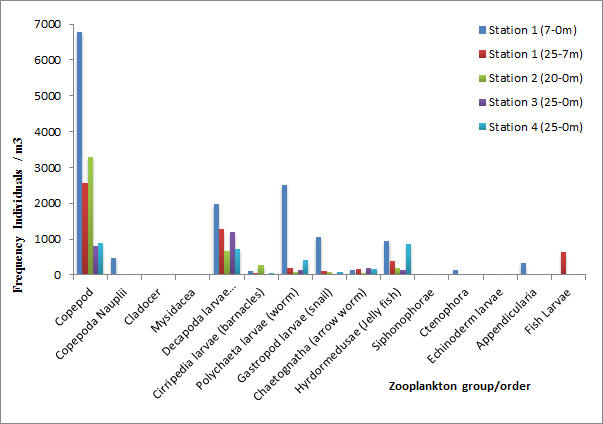
Figure 14 (above) shows the community makeup of zooplankton at each station.
Discussion (Back to top of Offshore Boatwork, webpage)
Physical - Thermal and Salinity structure
The offshore data collected showed a wide variety of physically varied profiles between stations with regards to temperature and salinity. The first station was to the south of Black Rock at the mouth of the Fal estuary. The depth profile showed stratified conditions with warmer, fresher water at the surface gradually decreasing and increasing in temperature and salinity respectively. This is unexpected for this station as the large tidal flow is expected to cause instability and turbulence that hinders stratification of the water column and causes vertical mixing.
Overall, the surface temperatures of each station were within the range of 12 to 140C. Further away from the coast, most notably at stations 3 and 4 where tidal mixing has less effect, a much more stratified water column was observed with a maximum difference of surface temperature and temperature at depth to be 20C with a salinity change of 0.2 at station 4. The change in temperature and salinity mainly occurs between 20 and 30m of depth, where the thermocline is situated. Its position within the water column changes with the seasons, and it is currently at an intermediate depth as we approach the summer season. The thermocline aids in the stratification and higher stability of the water column which is also an important factor for primary production (Hollidaya et al 2006 p.g. 201).
The location where stratified and mixed water masses meet is known as a front. One of its main characteristics is the position of the thermocline which reaches the surface at the frontal system. This is caused by the well mixed water mass meeting the stratified water mass and pushing the thermocline upwards. This results in surface currents parallel to the front and very sharp horizontal temperature, salinity and turbidity gradients. Station 4 shows that the thermocline is slightly shallower in depth than station 3, which may suggest that the thermocline is gradually being pushed upwards. Though rough conditions on the day made sampling beyond station 4 difficult, perhaps satellite imaging could help with the identification of the frontal system to the east of the Fal Estuary.
ADCP/Richardson’s Number
A front occurs due to stratified waters meeting well mixed water which causes the thermocline to be pushed upwards towards shallower depths. As the mixing depth gets closer to the surface, thermal stratification breaks down.
At our sampling stations, there is strong evidence of stratification in the water column. However, as rough weather prevented us from going to further stations for sampling, we did not locate the front. If we did locate the front, we could expect to see that the velocity in the stratified region before the front to be greater. This is because it is separated by the density and temperature difference from bottom friction of the increasingly shallower seabed which would slow it down. On the mixing side of the front, it can be expected that velocities would be slowed by the mixing and friction of the seabed.
On the stratified side of the front, the distribution of the Richardson’s Number would be very similar to that at the mouth of the estuary and at the station closer to the coast which is also stratified. The Richardson’s Number profiles for all the stations show very high Richardson’s Numbers in the depths between the thermocline and the surface and at the depths between the thermocline and the seabed. This is due to the fact that mixing in these depths is laminar and that the water mass here is stable. Where the thermocline lies in the water column, the Richardson’s Numbers are below 0.25 which means there is turbulent mixing taking place between the stratified layers (Mack and Schoeberlein 2004).
If a front was located on our day of sampling, the ADCP data would show a clear patch of phytoplankton in the stratified area. Before a decrease in depth there would be a breakdown in the plankton which would follow the shape of an internal wave. This shape could be caused by a change in flow around shallow rocks as the depth decreases. Phytoplankton blooms in the thermocline are being fed on by the zooplankton that produces backscatter on the ADCP. Phytoplankton blooms beyond the front are due to daily changes in the tide which replenishes the stratified waters with nutrients and mixes phytoplankton to the surface where light intensity is the greatest.
Chemical
There is a general trend that phosphate increases with depth. Phosphate is used in primary production which can be light limited. When it is used up, it is replenished from the upwelling below euphotic depths. Stations 1 and 2 which are just outside the estuary have high surface values for phosphate as the less dense, phosphate rich freshwater leaves the estuary, but there is less phosphate at depth. Silicate follows a similar trend to phosphate. Silicate is a limiting nutrient for some primary producers such as diatoms. Both phosphate and silicate trends are mirrored by the phytoplankton trends which are most abundant where nutrients are being used, i.e. the thermocline. Fluorometer and chlorophyll data provide a proxy for phytoplankton abundance. Phytoplankton are also limited by the base of the euphotic zone which is calculated from the Secchi depth and is normally quite shallow. The trend of high phytoplankton abundance within the thermocline compared to surface waters could be explained due to greater turbulence at the surface. Unexpected values for dissolved nutrients may be due to movement of phytoplankton in the water column, such as phosphate levels at station 4 which show a maximum below the thermocline.
Phytoplankton blooms in surface waters tend to be sporadic and short lived as they become nutrient limited. However in the thermocline nutrient levels are higher due to upwelling from the mixed layer but light intensity is still high enough for primary production and thus more sustained abundance is seen. The summer thermocline prevents upward mixing of recycled nutrients and so limits growth in surface waters.
All stations show high dissolved oxygen levels which increases with depth. This matches the fluorescence data which is a proxy for chlorophyll and phytoplankton, as increasing dissolved oxygen infers increasing primary productivity, which reaches a maximum at the thermocline. This is also in line with the phytoplankton counts which show a higher abundance of phytoplankton occurring at the thermocline at intermediate depths.
Biological
Phytoplankton
There are a number of factors that can determine changes in phytoplankton levels. Phytoplankton photosynthesise using chlorophyll to absorb sunlight and convert this into chemical energy. Their abundance therefore depends on the amount of light available whilst also depending on their other sources of energy, such as dissolved nutrients. The western English Channel is an especially interesting region to study because it is situated on the border of cold and warm temperate waters, whilst also bridging oceanic and neritic waters (Southward et al., 2005).
It can be seen that dinoflagellates are very few in number compared to the number of diatoms, which is unusual for this time of year. Diatom blooms occur in spring followed by a dinoflagellate dominant water column in the summer on the northwest European continental shelf (Maddock, et al., 1981). Between June and August, dinoflagellates should dominate at the thermocline prior to a second diatom bloom in September when the thermocline subsides (Holligan and Harbour, 1977). However, the phytoplankton counts show a different story, as it is possible that stormy weather during early June has had an impact on the stability of the water column in these coastal waters.
Diatom blooms occur in spring due to full vertical mixing that stabilises the water column; high winds in early June has caused the water column to stay more mixed and less favourable to dinoflagellates which reside in the thermocline. However, as seen in the CTD profiles, stations 3 and 4 are more stratified than the other two stations. As a result, phytoplankton counts show the highest number of dinoflagellates at stations 3 and 4 at intermediate depths (i.e. at the depth of the thermocline), numbering more than diatoms.
Zooplankton
Overall it is seen in the data that copepods are the most abundant group in the sampling area, which correlates with other studies in south-western English waters where large spring blooms are seen (Wishner et al 1988). Other groups such as decapoda/polychaetae larvae and hydromedusae have reduced but significant frequencies. The main issue with this analysis is that it is a very subjective method of identifying different zooplankton orders and groups especially when working in a large group of people. This could explain the general peak in values seen at Station 1 for depths of 0-7m, compared to the other stations as the observer may have been more thorough or have had a different method of identification.
The dominance of copepods seen in the offshore survey falls in line with observations that have been taken since 1988, at the L4 station off Plymouth. Zooplankton analysis by the Western Channel Observatory is of the major taxonomic groups, to which copepods, especially calanoid copepods have played a major part (web reference). Similarly, hydromedusae being dominant in the offshore survey, mirroring observations already made in the Western English Channel. This was seen by Vallet and Dauvin (1999), after a survey of zooplankton in the Western English Channel was carried out through the months. It was seen that in June cnidarians in general were the third most dominant zooplankton group.
Estuarine Boatwork - Materials and Methods, Results (back to top of webpage)
An estuary can be defined as a semi-enclosed coastal body of water which has a free connection with the open sea and within which sea water is measurably diluted with fresh water derived from land drainage (Pritchard, 1967). All estuaries have a head where fresh riverine water enters and a mouth which opens to the sea, allowing for discharge and mixing between estuary and seawater.
Estuaries tend to be quite polluted bodies of water due to the high amount of anthropogenic activities that take place around and on them; including fishing and other boat activities, sewage, waste disposal and in particular the discharges from industrial activities. Pollution tends to raise the nutrient level of the water meaning that phytoplankton and bacterial growth will be accelerated. This can cause eutrophication of the water column in an estuary resulting in a decrease in the oxygen saturation of the water, which will damage ecosystems and can cause the death of organisms. In terms of the Fal estuary it is classed as a polluted body of water with high levels of heavy metal pollution such as copper, tin, zinc and arsenic due to discharges from previous mining efforts in the area (Pirrie et al, 2003).
Restronguet Creek the tidal ria is a tributary of the Fal estuary around 5km north of Falmouth. It consists of several areas, which are heavily polluted especially in terms of Copper concentrations that have been shown to induce increased tolerance to copper in polychaetes such as Nereis diversicolor (Milward, Grant 2000). This could have an influence on the pollution level of the Fal and is something we will investigate during our boatwork.
The aim of our investigation of the Fal estuary is to gain understanding of the chemical, physical and biological factors of the estuary and how they change over a specified area, ranging between the riverine and seawater end members. This will be accomplished with a variety of different instruments during our time on the Bill Conway: A CTD will be deployed at each station to measure the salinity, turbidity, temperature and fluorescence throughout the water column. An ADCP will also be used to gain an understanding of the flow and its velocity at each station as a horizontal transect. A Niskin bottle on a hydroline will be used to collect a representative set of water samples which can then be taken back to the lab to determine the concentration of chlorophyll, dissolved oxygen, silicon and phosphate. A transmissometer on the CTD will be used to measure the change in light through the water column at each station in conjunction with a Secchi disk so that the base of the euphotic zone can be estimated. In addition to these langrangian measurements we have also collated a series of eularian results for the estuary from work at the King Harry Ferry pontoon.
Aside from Restronguet Creek the Rivers Truro and Kennel amongst others discharge into the estuary and are major sources of estuarine nutrient input. Nutrients are necessary for phytoplankton growth and thus the river discharges and sources of pollution along the estuary can cause phytoplankton blooms. During our field course the estuary is moving from spring into summer and therefore the water column should have warmed (despite the poor weather) resulting in formation of a thermocline. The thermocline will aid in the stabilization of the water column meaning that phytoplankton will be suspended in the euphotic zone for a greater period of time increasing their productivity and numbers. We therefore expect that results will show a bloom of phytoplankton so long as nutrients have not been depleted. We would also expect to see a significant increase in zooplankton numbers (such as copepods) in response to the greater prey levels, presuming that the lag period for their response to the change has passed.
From a chemical point of view our interest will be focused on how the concentrations of constituents in the water column change as we move between the riverine and seawater end members assuming that the end members will remain constant during sampling. If an element is behaving conservatively then we would expect the concentration changes to plot as a straight line between the two end members. Conservative behaviour is associated with conditions where nutrients are neither being added nor removed and concentration is determined at any one point by the mixing of riverine and seaward waters to varying degrees. Non-conservative behaviour (data points not adhering to a TDL) suggests that nutrients are either being removed (data dipping below TDL) or added. Addition and removal of nutrients can be caused by either physical processes (heavy rainfall increasing run off, re-mineralization etc) or by biological processes such as phytoplankton blooms (e.g. diatoms up taking silicon for creation of skeletal material).
The physical parameters that were investigated during our sampling should reflect the main forcing for the Fal which is in this case tidal. The tidal range is variable with macrotidal conditions being seen at the mouth and at Falmouth but mesotidal towards the mid-estuary and Truro (spring 3.5m). Although not the greatest tidal range this will cause significant mixing so that a salt-wedge type estuary should not be seen. However, whether it will result in a fully homogeneous and well mixed water column remains to be seen and most probably a mix between the two will be present (partially mixed).
Materials and Methods - (back to top of Estuarine Boatwork/webpage)
 Due to the limited time frame we sampled with the tide instead of
against it. Scientifically it would have been better for us to sample
against the tide so we wouldn’t be sampling the same water mass. However
this was not a possibility and we will use the changes in salinity
through the estuary to see how the water masses change.
Due to the limited time frame we sampled with the tide instead of
against it. Scientifically it would have been better for us to sample
against the tide so we wouldn’t be sampling the same water mass. However
this was not a possibility and we will use the changes in salinity
through the estuary to see how the water masses change.
The sampling of two depths at Station one occurred due to the water depth being very shallow. The O2 , Si, N +P and Chlorophyll were all parameters sought from the retrieval of water from the depths mentioned above. Oxygen was stored in a labeled glass bottle. This was the first measurement taken. Plastic tubing attached to the Niskin provided the oxygen sample which was filled to the top and overflowed to truth the oxygen values. This then required the addition of 1ml of Manganous Chloride and 1ml of Alkaline Iodide the bottle capped and stored in a bucket filled with seawater.
A large jug of water was then used to collect the remaining water inside the Niskin, from this we used a syringe (washed through with a small volume of the water from the jug) to measure 50ml. The syringe was then attached to prepared filters. A small volume passed through the filter to ensure the same consistency of fluid throughout. The Silicon labeled bottles were then attached to the filter and washed through with a small amount of sample before adding the remaining 50 ml into the bottle. The Fiber glass filter was then retrieved from the filter and placed in labeled test tubes containing acetone (for Chlorophyll).
Brown bottles were used for the storage of Phosphate + Nitrate. This required the extraction of a further 50ml of sample, attached to a filter (washed through with a small volume of the sample 1/2ml) The brown bottle was then washed through with 1/2ml when attached to the filter. The remaining 50 ml then filtered into the brown bottle. The removal of the fiber glass filter meant that we had a second Chlorophyll measurement. The Filter was too placed into a labeled test tube containing acetone.
A brown-labeled bottle containing lugosiodide was used to preserve the phytoplankton. We poured 2 X 50ml of the sample retained from the Niskin bottle into the brown bottle containing lugosiodide. We did not extract using the syringe, but removed the plunger from the syringe and added the water directly into the syringe to ensure no damage to the phytoplankton through the small ending of the syringe. This was carried out for the surface depth only. The Temperature and Salinity was logged for each water sample at the various depths.
Chemical analysis as described for station 1 was carried out for station 2 using the exact same protocols. An additional 3 depths were measured here therefore there was 3 more bottles for analysis for each parameter. Phytoplankton analysis was carried out for the surface depth only.
Chemical analysis as described for station 1 was carried out for station 3 using the exact same protocols. An additional 2 depths were measured here therefore there was 2 more bottles for analysis for each parameter. Phytoplankton analysis was carried out for the surface depth only. For the surface sample two bottles were taken for 02 analysis.
Underway samples were taken in between stations. These were taken with a change in 1.0 salinity unit in the water mass. This was determined taking the values from the T/S probe attached to the underway pump.
Samples from the underway were analysed as described at each station however nutrient information was required for Si, N +P and Chlorophyll and therefore no measurements were made for O2 or phytoplankton.
The Zooplankton Tows were carried out at Station 1 and 3 only ,using a tow with 50cm diameter and 210μm mesh.
The Zooplankton samples required the addition of 10ml of formalin to the bottle to ensure preservation for further analysis in the onshore laboratory.
Meta Data
Research Platform: R.V. Bill Conway (see figure X - right)
Weather Conditions: Sunny, fair wind, 5/8 cloud coverage.
Sea State: Calm except at river mouth where was a little choppy.
| Time GMT | Tidal Height (above chart datum) | |
| Low Water | 01:31 | 0.30m |
| High Water | 07:09 | 5.00m |
| Low Water | 13:52 | 0.30m |
| High Water | 19:26 | 5.30m |
Table 2 is a tidal chart for the Fal Estuary - 05.07.2012
CTD Cast Sites
Station 1
|
Time (UTC) |
09:07 |
|
Latitude |
50° 14.391 N |
|
Longitude |
5° 00.885 W |
|
Depth (m) |
5,5,5,5,5 – repeats done due to anomalous salinity values |
|
Bottom Depth (m) |
7,7,7,7,7 |
|
Salinity |
32.5 |
|
Secchi Depth (m) |
1.1 |
Station 2
|
Time (UTC) |
10:02 |
|
Latitude |
50° 12.182 N |
|
Longitude |
5° 02.419 W |
|
Depth (m) |
14 |
|
Bottom Depth (m) |
17.2 |
|
Salinity |
35.992 |
|
Secchi Depth (m) |
2.1 |
Station 3
|
Time (UTC) |
11:03 |
|
Latitude |
50° 08.735 N |
|
Longitude |
5° 01.446 W |
|
Depth (m) |
20,20 |
|
Bottom Depth (m) |
33,33 |
|
Salinity |
36.879 |
|
Secchi Depth (m) |
5.0 |
Niskin Bottle Hydroline sites
Station1:
Latitude: 50° 14.319 N
Longitude: 5° 00.885 W
Water Sampling Depths (m): 1, 5
Time: 08:53 UTC
Station2:
Latitude: 50° 12.182 N
Longitude: 5° 02.422 W
Water Sampling Depths (m): 1, 3, 5, 7, 9
Time: 10:06 UTC
Station3:
Latitude: 50° 08.716 N
Longitude: 5° 01.463 W
Water Sampling Depths (m): 1, 3, 6, 9
Time: 11:09 UTC
Underway Samples - taken every 1 PSU change in salinity via onboard pump while moving
Sample 1
Latitude: 50° 14.104 N
Longitude: 5° 01.130 W
Time: 09:36 UTC
Salnity:29.2
Temperature (oC): 15.4
Sample 2
Latitude: 50° 13.725 N
Longitude: 5° 00.964 W
Time: 09:42 UTC
Salnity:30.1
Temperature (oC): 15.2
Sample 3
Latitude: 50° 12.487 N
Longitude: 5° 01.785 W
Time: 09:56 UTC
Salnity:31.8
Temperature (oC): 14.8
Sample 4
Latitude: 50° 12.487 N
Longitude: 5° 01.785 W
Time: 10:57 UTC
Salnity:34.6
Temperature (oC): 13.5
ADCP Cross Section Sites
Cross Section 1
|
|
START |
END |
|
Time (UTC) |
09:28 |
09:32 |
|
Latitude |
Missing data |
50° 14.329 N |
|
Longitude |
Missing data |
5° 00.858 W |
Cross Section 2
|
|
START |
END |
|
Time (UTC) |
10:28 |
10:34 |
|
Latitude |
50° 12.175 N |
50° 12.042 N |
|
Longitude |
5° 02.597 W |
5° 02.108 W |
Cross Section 3
|
|
START |
END |
|
Time (UTC) |
11:39 |
12:49 |
|
Latitude |
50° 08.534 N |
50° 08.534 N |
|
Longitude |
5° 01.027 W |
5° 02.273 W |
Zooplankton Trawl sites
Station 1
|
|
START |
END |
|
Time (UTC) |
09:23 |
09:28 |
|
Latitude |
50° 14.328 N |
50° 14.400 N |
|
Longitude |
5° 00.920 W |
5° 00.864 W |
|
Flow |
50382 |
50941 |
Station 3
|
|
START |
END |
|
Time (UTC) |
11:29 |
09:28 |
|
Latitude |
50° 08.614 N |
50° 08.468 N |
|
Longitude |
5° 01.582 W |
5° 01.504 W |
|
Flow |
50941 |
51458 |
Results (back to top of Estuarine Boatwork/webpage)
Physical
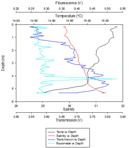
Figure 15 (above) shows the depth profile of the CTD data collected at Station 1.
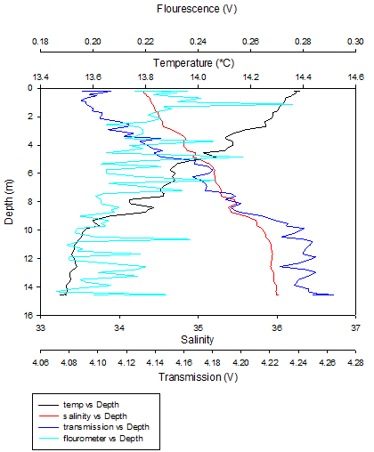
Figure 16 (above) shows the depth profile of the CTD data collected at Station 2.
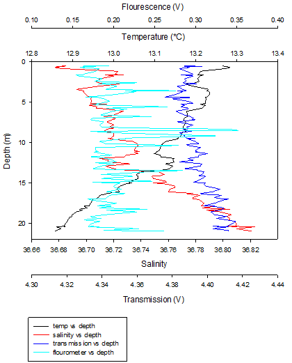
Figure 17 (above) shows the depth profile of the CTD data collected at Station 3
Richardson's numbers
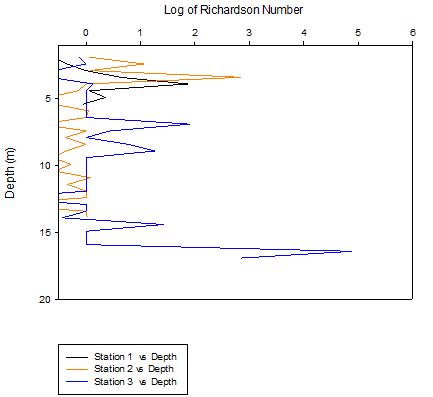
Figure 18 (above) shows the difference in Ri with depth for all 3 estuarine stations.
Residence Time of Fal Estuary
The equation below uses the value of flow rate as an average from past years (1978-2010) for July.

Where; Tres = residence time
Smean = mean salinity of the estuary from calculating mean of all salinity values recorded in estuary (stations 1, 2 and 3): 33.5
Ssea = Salinity of sea, average of values recorded at the sea end member station: 35.15
Vtotal = total volume of the Fal Estuary: 1.35x10⁷m3
R = the flow rate of the Fal Estuary: 2.028m3s-1 CITATION 48012 \l 2057 (48003 - Fal at Tregony)

![]()
![]()
![]()
Flow rates of the major riverine inputs of the Allen and Kenywn Rivers result in a residence time in the estuary of 3.62 days. This model is simplified and therefore an estimation of residence time as several assumptions are made for it to work. It is assumed that there are no other freshwater inputs from geological sources other than the river itself (i.e. no groundwater discharge) and doesn’t take into account any meteorological influences (i.e. rainfall). This summer’s rainfall has been dramatically higher than in previous years, however our model relies on prior years average flow rate (1978-2010) in order to be calculated and therefore results may be skewed.
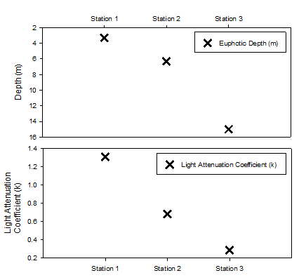
Figure 19 (above) shows the calculated euphotic zones from both secchi disk depth and from CTD irradiance data.
Chemical
Nitrate
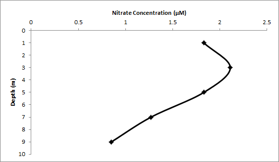
Figure 20 (above) shows the change in nitrate concentrations for Station 2.
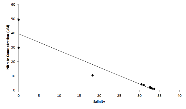
Figure 21 (above) shows an estuarine mixing diagram for nitrate with a TDL.
Silicon
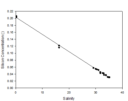
Figure 22 (above) is a mixing diagram including a TDL for dissolved silicon (silicic acid)
Chlorophyll and dissolved O2 results
At station 1, the most upstream station, chlorophyll increases with depth while oxygen saturation decreases with depth. Chlorophyll concentration increases from 3.59 to 4.48µg/L while oxygen levels decreases from 96.76 to 96.13% saturation.
Station 2 sees chlorophyll concentrations increasing with depth with a maximum chlorophyll concentration of 3.3360µg/L at 3m, which then decreases slightly with depth to 3.18µg/L at 5m and 3.162µg/L at 7m. Oxygen saturation decreases slightly from the surface down to 3m and then increases rapidly from 3m down to 7m with a highest percentage saturation of 110.696 at 7m.
At station 3, the most seaward station at the mouth of the estuary, oxygen levels increase between 1 and 3m from 96.3185 to 97.2435, and then increase again from 3m to 6m up to a level of 97.5013% saturation. Oxygen levels then fall dramatically from 6 to 9 m down to 93.9951% saturation. Chlorophyll levels decrease with depth from 2.980 at 1m down to 1.0818 at 6m, before increasing slightly to 1.1682 at 9m.
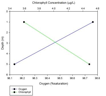
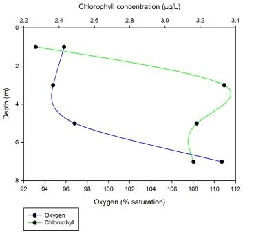
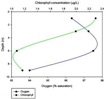
Figure 23 (top left) is a plot of how the chlorophyll concentrations and dissolved oxygen concentrations from the discrete water samples changed with depth at station 1.
Figure 24 (top right) is a plot of how the chlorophyll concentrations and dissolved oxygen concentrations from the discrete water samples changed with depth at station 2.
Figure 25 (bottom left) is a plot of how the chlorophyll concentrations and dissolved oxygen concentrations from the discrete water samples changed with depth at station 3.
Biological
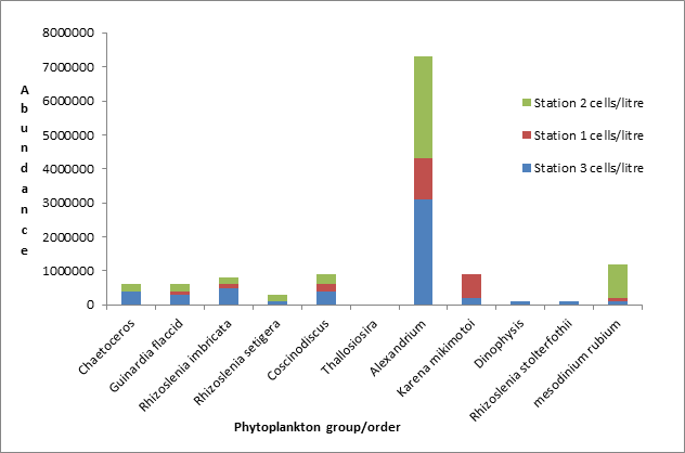
Figure 26 (above) shows total phytoplankton abundance and how individual community structure changes with station.
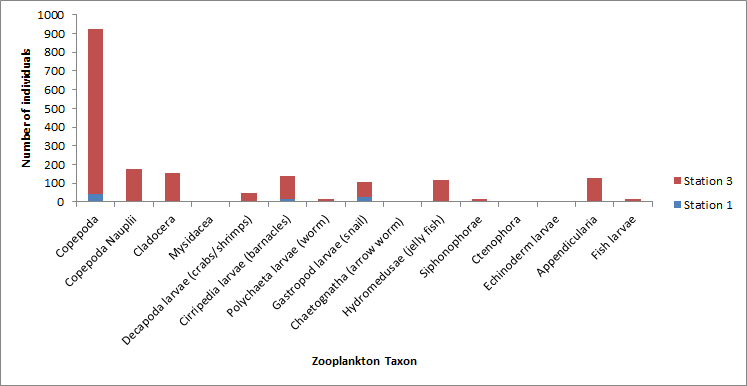
Figure 27 (above) shows the relative number of different species of zooplankton for each station.
Physical
CTD data for station 1 (upper estuary) shows a trend of fresher water near the surface overlying saline waters, which reach a salinity of 31.5 around a depth of six meters. The salinity profile at station 2 shows a similar but slightly more saline profile with maximum salinity of 34.5 at 36m depth, indicating that the bottom water is completely saline as the maximum salinity is similar to that of the seawater end member. At station 3 the salinity structure changed to a profile dominated mainly by fully saline bottom water. Surface freshwater dilution was still evident but to a much lesser extent. The presence of a slight halocline across a small range of salinities in all three profiles indicates that the estuary is a partially mixed. The dominant forcing agent at the mouth of the estuary changes from tidal at the mouth to mesotidal towards Truro. Tidal action causes mixing of the water column and reduces its stratification. There is a possibility that spring/neap tidal cycles may skew results and this would need further investigation.
Figure 18 shows Richardson values throughout the water column for stations 1, 2 and 3 to be fairly high and consistently above 1. This shows a shear force insufficient to overturn the water column, resulting in the stratification of the water column seen in the CTD salinity profiles. The low and 0 values in the graph are due to pockets of less dense warmer water located in mainly denser areas of the water column. The inference of stratification from this data agrees with the stratification observed through water column sampling at Blackrock in the offshore work.
CTD Transmissometer values from station 1 show and increase in turbidity with depth, with a maximum of 3.8 volts at 5m depth, indicating higher levels of suspended sediment near the estuary bed. Station 2 shows a similar pattern with slightly higher values due to higher velocity flow from the sea suspending greater amounts of sediment. Turbidity increases slightly at station 3 but is more consistent throughout the water column possibly due to the timing of measurements coinciding with the flooding of the tide.
As we moved down the estuary the euphotic depth measured by Secchi disk increased from a depth of 3.3m at station 1 to 15m at station 3. The light attenuation coefficient decreased towards the lower estuary, reaching a minimum of 0.288 at station 3. This indicates that light is absorbed more rapidly in the upper estuary compared to the lower estuary where it penetrates much deeper. This is probably due to greater sediment input in the upper estuaries from river water.
These findings are contradictory to those from the CTD transmissometer readings, which suggest that there is greater turbidity at stations 2 and 3, so there is greater suspended particles in the water column at these stations which would be logical due to finer sediments in mid estuary locations combined with greater flow rates due to tides.
.
Nutrients
The estuarine mixing diagram for silicate shows points with little deviation from the Theoretical Dilution Line (TDL). This indicates that dissolved silicon was acting in a conservative manner throughout the estuary and was not affected by significant biological uptake from organisms such as siliceous Diatoms. This implies that the main factor controlling the distribution of silicon along the estuary was the mixing water masses. Concentrations of silicon decrease down the estuary as the silicon rich riverine water body mixes with and is diluted by the seawater. Seawater contains little silicon as a most inputs come from weathering of terrestrial rocks and biological activity in the oceans may remove high proportions of it from the water column.
Although the behaviour of silicon was shown to be conservative, low rates of biological removal could have been occurring alongside the mixing of the water masses. Turbidity in the water column was shown to be high from the CTD results and this could have affected phytoplankton growth and usage of the silicon as available light would have been reduced. In addition to this the water in the past few weeks during and before our time of sampling has been poor. This may have slowed the formation of the thermocline, reduced light levels and generally created conditions that are poor for blooms to occur under. Also there may be high zooplankton numbers in response to an earlier spring bloom that are controlling phytoplankton growth.
Nitrate concentration decreased as we moved down the estuary and displayed a slightly non-conservative behaviour. Figure 21 shows that there is removal at a salinity of 18, indicating a small degree of uptake of nitrate by phytoplankton. Uptake by phytoplankton was seen to be minimal, although at other times of the year and during better weather conditions nitrate may be depleted and exhibit non-conservative behaviour. Figure 20, a nitrate depth profile taken at Turnaway point, shows a slight increase in concentration from surface to 3m followed by a decrease to a minimum value of 0.85um at 9m.
Non-conservative behaviour of phosphate was also seen in the estuary as points bow away from the TDL. Between the salinities of 15 and 20 there appears to be addition of phosphate into the estuary, the exact source is unknown but it is possible it could have come from input of industrial effluent or sewage outlets.
The phosphate depth profile from Turnaway point shows a similar pattern to that of nitrate. An initial increase in concentration from the surface to 3m is followed by a continuous decrease from 3m onwards. This similarity considered alongside the similarity in non-conservative behaviour of phosphate to nitrate indicates that the similar controlling factors, namely phytoplankton abundance and weather conditions, influence the concentrations along the estuary.
Biological
There is a peak in fluorescence of about 0.53 volts between 4 and 5 meters. Chlorophyll concentration measurements obtained from chemical analysis of a water sample taken at 5 meters show an increase from surface levels. These measurements all indicate there to be higher phytoplankton abundance at around 5m. Oxygen concentrations calculated from water samples taken show a decrease with depth, which suggests that the turbidity levels may be inhibiting the ability of the phytoplankton to photosynthesise
Chlorophyll concentrations from water samples showed that there is more phytoplankton present in the water column. Coupled with this oxygen levels also increase with depth, suggesting that greater levels of phytoplankton biomass lead o an increase in oxygen in the water column due to oxygen production through photosynthesis. The CTD data however does not concur with the water samples taken for fluorescence levels at station 2, as they show a slight decrease in fluorescence and so chlorophyll concentration with depth.
Fluorescence from the CTD profile of station 3 is again constant throughout the water column but with higher values between 8 and 10 meters indicating a high phytoplankton abundance at this point. Oxygen from water samples was shown to decrease with depth at station 3 as was chlorophyll although a slight increase can be seen at 8 meters which correlates with our CTD results.
The phytoplankton abundance for the estuary is shown here in Figure 26 with stacked bars representing each of the 3 different stations. Alexandrium is the most abundant phytoplankton group at all stations, far exceeding all others with a maximum number of 3100000 cells per litre at station 3. Alexandrium is a dinoflagellate genus of phytoplankton that is often associated with toxic bloom events. We may have seen such large abundance due to the temperature of the water as this species has a very specific window of conditions for cyst development, and the weather was during measurements unseasonably cold (Anderson 1998 p.g. 32). Many of the other phytoplankton groups tend to show a similar abundance at each station, much lower than that of Alexandrium. Chaetoceros and Rhizoslenia setigera are absent from station 1 and Thallosiosira was not seen at any of the stations. In general the abundances seen are fairly low and this could be explained due to a lack of surface nutrients. During our time of measurement the light levels or irradiance should be high as it is the spring to summer period and therefore should not be limiting although the weather was not as such and so light could well of been a limiting factor during this period.. Also the water column should be fairly stable due to heating and the development of a thermocline meaning that phytoplankton should be held in the euphotic zone which is necessary for growth. However nutrients may have been depleted by an earlier spring bloom meaning that the primary producers may now be nutrient limited explaining their low numbers with the exception of Alexandrium.
In conclusion from the water sampling of the Fal estuary we found that it has partially mixed salinity structure with vertical stratification which traps nutrients at the thermocline, supporting higher populations of phytoplankton in the euphotic zone. Greater populations of phytoplankton are found at the lower end of the estuary, due to conditions of low turbidity combined with nutrient inputs from riverine water. These in turn supported an increased zooplankton population in the same area. However, this is only a reflection of the Fal estuary at the time of survey as its physical, biological and chemical characteristics can be expected to vary between seasons, daily tides and spring and neap cycles.
Pontoon Sampling - Materials and Methods, Results (back to top of webpage)
The aim of the data sampling undertaken on the pontoon was to assess the water quality and variability across a time series. The location of the pontoon was next to the King Harry Ferry crossing on the Fal Estuary. This location is tidal, so the time series will show the change of the water conditions with the rise and fall of the tide. The variables measured were the temperature, salinity, acidity, chlorophyll concentration and oxygen saturation using a YSI probe and reader, the light attenuation using a light sensor and the current velocity and direction with a current meter. All were measured against depth every 15 minutes.
Date: 29/06/2012
Time: 09:00 – 12:45
Weather: cloud cover – <90% Very strong winds
King Harry Ferry
Latitude: 50°21’66N
Longitude: 05°02’77W
High Tide: 00:56BST (4.50m), 13:38BST (4.40m)
Low Tide: 07:38BST (1.30m), 20:10BST (1.30m)
Materials and Methods (back to top of Pontoon Sampling/webpage)
The instruments used include a YSI Probe (650 MDS), which measures temperature, salinity, pH, depth, chlorophyll concentration and oxygen saturation, where measurements were taken every metre at 15 minute intervals. A Li-1400 was used to measure light penetration at different depths to work out the light attenuation coefficient. Measurements were taken every metre at 15 minute intervals and the corresponding value from the surface probe was taken. Water samples were taken hourly using a Niskin Bottle from the surface and at the estuary bed. 50 ml of each sample was filtered through a glass fibre filter. The filters were then stored in numbered bottles with acetone for fluorescence measurements in the laboratory. A current meter (Valeport F66D) was deployed to look at the flow of water past the pontoon every metre at 15 minute intervals, with the speed and direction of flow measured.
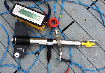
Niskin bottle (right)
As described above. During fieldwork on the pontoon, a Niskin Bottle was used to take water samples at the surface and at the bottom of the water column for hourly intervals to measure fluorescence and conversion to chlorophyll concentration for comparison with the values from the YSI Probe.
YSI (650 MDS) Probe (right)
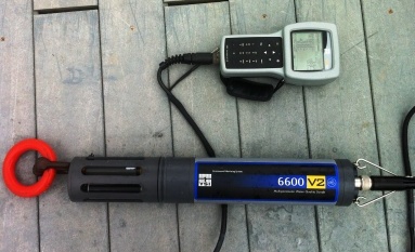
A YSI Probe is a multi-parameter probe that simultaneously measures conductivity (salinity), temperature, depth, pH, turbidity, oxygen saturation, and chlorophyll concentration. It was used for fieldwork on the Pontoon to measure physical and chemical changes in the estuary every metre in depth during a tidal cycle.
Current meter (Valeport F66D) (right)
A current meter is a device that is able to provide direct measurements for current velocity and direction, through the use of two pairs of titanium electrodes located symmetrically on the equator of the sensor, while an internal flux-gate compass provides heading direction. During fieldwork on the Pontoon, the current meter was deployed to measure direction and velocity of water running past the pontoon.
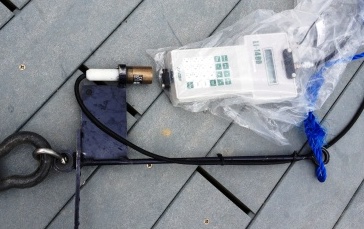
Li – 1400 Data logger (right)
A data logger fitted with a photosynthetic active radiation (PAR) sensor was used to measure the PAR at every metre in depth and the corresponding value at the surface for comparison during fieldwork on the Pontoon.
Results (back to top of Pontoon Sampling/webpage)
Temperature
Figure 27 shows a contour plot of temperature values collected on the pontoon by the King Harry Ferry on the Fal Estuary. Temperature values were highest at low tide times with warmer surface waters and cooler, denser waters at depth. However, during high tide there is evidence of a well mixed water column which is in the magnitude of a degree cooler due to seawater inputs. The contour plot suggests water introduced by the river is warmer than seawater inputs.
Salinity
Figure 28 shows a contour plot of salinity values collected on the pontoon by the King Harry Ferry on the Fal Estuary. Low water was at 7:38 BST, which is reflected in the plot from 9:00 to 11:00 BST where relative riverine input of water into the estuary is high and therefore lower salinities were measured in surface waters as it is of lower density and float on top of the higher density seawater underneath. As high tide was reached at 13:38 BST, salinity values increased as there is a higher relative input of seawater. The highest value recorded was at 12:45 of 34, this was maintained until the tide turned. There is also less vertical stratification as the tide mixes the water column. As the tide ebbed salinities decreased and stratification started to occur.
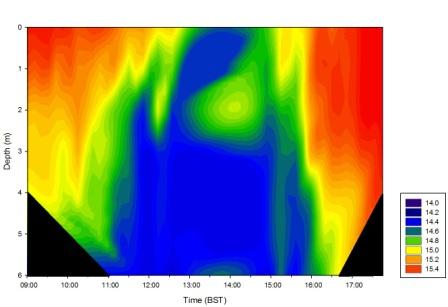
Figure 28 (above left) is a contour plot of changes in temperature with depth over the duration of the pontoon sampling.
Figure 29 (above right) is a contour plot of changes in salinity with depth over the duration of the pontoon sampling.
pH
Figure 29 shows a contour plot of pH values collected on the pontoon by the King Harry Ferry on the Fal Estuary. pH shows little variation due to tidal influence. There are slightly increased values in surface waters which penetrate slightly into the water column. An explanation for the limited variation in pH could be due to a fast estuarine tidal turnover time.
Chlorophyll
Figure 30 shows a contour plot of the chlorophyll concentrations off the pontoon by the King Harry Ferry on the Fal Estuary. Values in the bottom left of the graph are distorted as there was no data collected at 5 and 6 meters until the tide had come in sufficiently to measure to that depth. Especially high concentrations were measured during the period of high tide between 0.5 and 2m depth.
Figure 30 (above left) is a contour plot showing changes in pH with depth over the time of sampling.
Figure 31 (above right) is a contour plot showing changes in chlorophyll concentrations with depth over the duration of the period of sampling.
Dissolved Oxygen
Dissolved oxygen (figure 32) increases with time over the course of the day and is fairly homogeneous with depth.
Figure 32 (above) is a contour plot of the dissolved oxygen concentrations and depth over the duration of sampling.
The plot of irradiance (figure 33) shows how light attenuates throughout the water column. Irradiance levels are highest in surface waters and a decrease is seen with depth. In the middle of the contour plot reflects a change over of groups sampling and therefore no data was obtained between 12:45 and 14:30 BST.
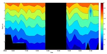
Figure 33 (above) shows irradiance with depth over the duration of the sampling period.
Discussion (back to top of Pontoon Sampling/website)
Temperature contour plot analysis shows when the tide is low surface water temperatures are highest, decreasing with depth. This reflects the presence of warmer less dense fresh water sitting on top of the water column below which the cooler more saline waters reside. This is further depicted in the salinity contour plot, which shows the fresher water with lower salinities sitting on top of the higher salinity saline water. At high tide saline water dominates, as there is strong tidal mixing causing vertical homogeneity throughout the water column. Similarly, at high tide temperatures are lowest due to inflow of cooler saline water from the sea into the estuary.
pH is of an alkaline nature, ranging from 8.6 to 8.9. It is homogeneous throughout the water column and shows great consistency throughout the tidal cycle. However, chlorophyll levels show a maximum during midday in surface waters when solar irradiance levels would be highest and phytoplankton have maximum sunlight available for photosynthesis. At the King Harry Ferry pontoon, the water column is not deep enough to incur a 1% light depth therefore chlorophyll values are found up to maximum depth as there is still sufficient light for chemical and biological processes to occur.
Dissolved oxygen levels at the beginning of the tidal cycle are shown to be lowest as they will have been depleted overnight by respiring organisms, as photosynthesis is not possible in the absence of light. It is shown to be at a maximum at 17:00 BST as accumulation of oxygen will have occurred as a bi-product of photosynthetic activity throughout the day.
Irradiance levels were highest in surface waters as expected as sunlight penetrates easily into this layer. However, with depth, light is scattered by suspended particles preventing the passage of light to depth. Towards the afternoon there is less irradiance throughout the water column as a direct effect of the sun setting.
Technical difficulties with the current meter meant that our group was unable to obtain data sufficient for analysis.
Geophysical Boatwork - Materials and Methods, Results, Discussion (back to top of webpage)
The Fal estuary contains multiple types of marine environments such as sheltered intertidal mudflat, sand flat areas, large shallow inlets and bays, sub-tidal sandbanks, Atlantic salt meadows, reefs and estuaries - all of which are listed under protected ANNEX I habitats. The Fal Estuary is currently a designated SAC (Special Area of Conservation) mainly due to the presence of the calcareous algae maerl and seagrass beds. The maerl beds (Phymatolithon calcareum) found in the Fal Estuary are the largest in SW England and are host to a rich variety of epifaunal and infaunal species that live on, in or around the maerl, including the rare Couch’s goby Gobius couchi. There are also areas of Eelgrass meadow (Zostera marina) which are host to rich sub littoral sand invertebrate communities.
 The area of study is also a probable MCZ (Marine Conservation Zone).
MCZ’s are newly proposed marine areas that will protect rare species or
geological areas. However of the originally proposed 127 areas to be
protected, it is estimated there will most likely be a maximum of 33
accepted by the government due to financial constraints and the
difficulty of enforcing the legislation and policing the areas.
The area of study is also a probable MCZ (Marine Conservation Zone).
MCZ’s are newly proposed marine areas that will protect rare species or
geological areas. However of the originally proposed 127 areas to be
protected, it is estimated there will most likely be a maximum of 33
accepted by the government due to financial constraints and the
difficulty of enforcing the legislation and policing the areas.
A 2013 proposed dredging contract to create a new and improved channel into Falmouth Harbour is an operation that has the potential to negatively impact various species within the area. Sediment dispersed around the estuary from the forecasted dredging could smother the maerl, inhibiting their ability to photosynthesise leading to the death of the symbiotic algae and the deterioration of the maerl beds. It is estimated that there could be a net loss of about 4 hectares of maerl habitat and its faunal communities (falmouthport). The maerl and seagrass beds mentioned have specific biotopes: areas with defined environmental conditions and distributions of plant and animal life. Our investigation will identify biotopes in the area through the use of side scan sonar, grab analysis and video footage. If these biotopes prove to be particularly rare or important ecologically this could aid in the conservation of the area. The environmental impact of the dredging can be estimated and the survey should show areas that would be directly affected.
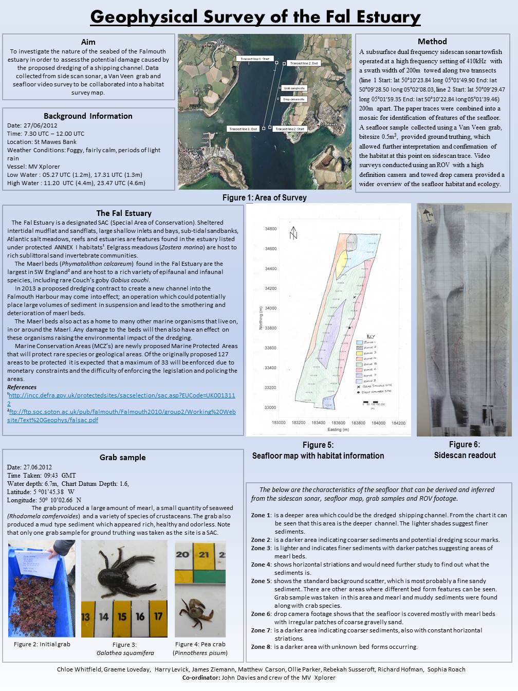
The aim of the geophysical survey conducted, was to investigate the nature of the seabed of the Falmouth estuary in order to assess the damage that could potentially be caused by the proposed dredging of a new shipping channel into Falmouth Harbour. Data for this survey was collected from a side scan sonar tow fish to scan the sea bed, a Van Veen grab to take samples of the sea bed and a drop camera and R.O.V. to perform a seafloor video survey.
A poster presenting the geophysical work undertaken was produced and is available below.
Materials and Methods (back to top of Geophysical Boatwork/webpage)
Sidescan sonar
The towfish transducer, which was towed from the ship, emits an acoustic sonar pulse which is reflected back from the seabed when it reaches the seafloor. The time between the emission of the beam and its return to the sonar receiver allows the sidescan computer to determine the distance and therefore the bathymetry. The acoustic strength of the backscatter received will vary depending on the type of sediment. Dense or very angular sediments provide the strongest returns.
Due to the survey site being shallow the dual frequency towfish was ran at 410kHz to give a high resolution while still maintaining a swath width of 200m (100m on either side of the fish. Two transects (detailed below) were completed and the traces of bathymetry data were combined into a mosaic to allow identification of features of the seafloor.
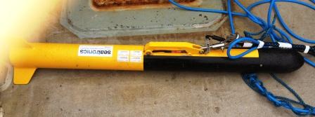
Figure 34 (above) is the sidescan towfish used on R.V. Xplorer.
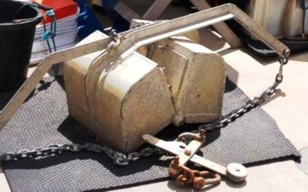
Van Veen Grab Sample
Only one grab sample was carried out due to the area being protected as a SAC. The grab sample was used to ground truth the seafloor, identifying the sediment type, and fauna and flora of the seabed at the chosen location. This ground truthing is important when using instruments such as sidescan as it allows the two forms of data to be compared to some extent.
Time Taken: 09:43 GMT
Water depth: 6.7m
Latitude: 5 °01’45.38 W
Longitude: 50° 10’02.66 N
Bite size: 0.5m3
Figure 35 (right): Van Veen Grab used to take a sample of the seabed
R.O.V. (Remotely Operated Vehicle)
The R.O.V "VideoRay" is fitted with two cameras, one standard resolution camera that can be turned for piloting purposes and a fixed, forward looking, HD camera to provide high resolution video and images of the underwater world. "VideoRay" also possesses two forward facing lights for illumination and thrusters to manoeuvre horizontally or vertically. The R.O.V. was connected to the onboard monitors via a neutrally buoyant cable which allows the R.O.V. to operate to a depth of 200m in favourable conditions.
R.O.V. footage provided a different perspective to the footage gained from the drop cam and due to the mobile nature of the R.O.V. we were able to cross reference the footage from the drop cam and provide a better overall view of the area. Additionally we were able to observe some marine life in situ including a rather awesome ray.
Particular thanks to Dr Adrian Glover of the Natural History Museum (London) for allowing the N.O.C. the use of the R.O.V.
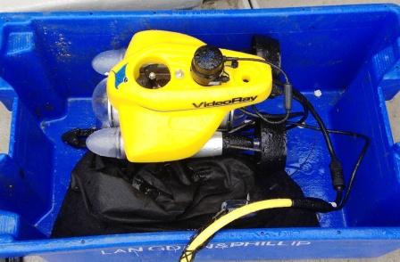
Figure 36 (above) is the High definition video R.O.V. "VideoRay"
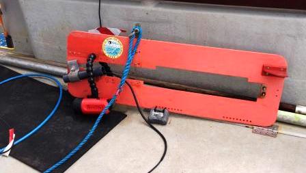
Drop Camera Video
The drop camera had a downward facing camera to visualize the seabed from above whilst being towed from the vessel via a line. Two lights were positioned to illuminate the field of vision of the drop camera for use in murky and darker conditions. The drop camera was used to further our knowledge of the seabed and allow us to draw comparisons using all three data sets.
Time Taken: 10.41 (GMT)
Water depth: 6.6m (Chart Datum depth of 1.6m)
Latitude: 50˚09’53.45N
Longitude: 5˚01’48.07W
Figure 37 (right): Drop Camera apparatus with which video footage was obtained and screen shots taken
Results (back to top of Geophysical Boatwork/webpage)
Sidescan Sonar
The side scan sonar produced a hard copy read out (Figure 38) from which zones of the varying seafloor characteristics could be identified and plotted using the program Surfer 8 (Figure 38).
From the trace alone we are only able to identify how the seafloor changes and any bedforms present within the surveyed area, as outlined in Figure 39. In order to provide confirmation of the characteristics identified along the seafloor, a Van Veen grab and drop camera video footage were used for ground truthing. We were able to identify the characteristics of zone 5, which extends throughout the majority of the surveyed area from 33000 m to 34400m Northing, using the grab sample. This indicated that the seafloor was comprised mainly of maerl beds, with some seaweeds and fine muddy sediments.
Drop camera video footage from Zone 6 (33200m to 34450m Northings, 183550m to 183700m Eastings) showed that the seafloor in this area was comprised of maerl beds and patches of exposed coarse sand and gravel. The darker areas seen in Zones 2, 7 and 8 indicate that the sediment is harder and coarser, whereas the lighter areas seen in Zones 1 and 3 indicate finer softer sediments.
Visible patterns and striations could be indicative of bedforms, natural or manmade from processes such as dredging, which is likely in Zone 1 and 2. However these are estimations at best and proper ground truthing methods would be necessary in each zone to accurately identify the seafloor in the survey area.
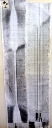
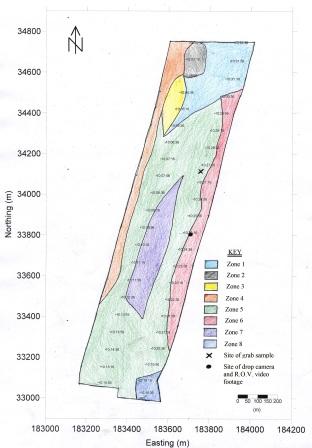
Figure 38 (above left) is the paper trace mosaic created from the original sidescan sonar printout. Features and boundary areas were drawn on and are visible in red. The significant darkening and bar like pattern towards the southward portion of the trace was due to deliberate operator variations in T.V.G. (time varied gain) in real time as the system we were using was analogue and showed an amount of variation with depth.
Figure 39 (above right) is the boundary map created from the analysis of the paper sidescan trace and includes marked sites for R.O.V and drop cam data and also the grab site.
Drop Camera and R.O.V.
The drop camera was deployed at lat: 50°09’53.45 N, long: 5°01’48.0714 W (Figure 30) at 10.41(GMT) to a maximum depth of 6.6m (Chart datum depth of 1.6m). The footage indicated that the seafloor at this location had 80-90% coverage of maerl bed, which was home to some species of seaweed (Figure 31). Based upon the grab sample results we believe the seaweed present in the drop camera footage to be Phodomela comfervoides. As we moved along from the original drop site the video footage showed areas where the maerl beds were patchy. Through these patches we were able to observe the seafloor sediment, which appeared to be comprised of course sands and gravel with some dead crustacean shells (Figure 32).
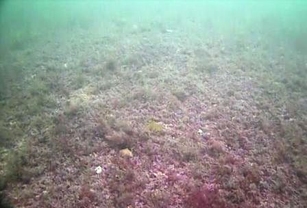
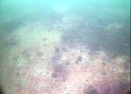
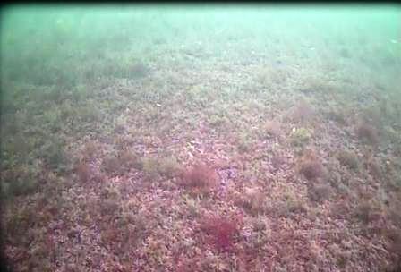
Figure 40 (below - left) is an still taken from the R.O.V. footage showing a healthy maerl bed.
Figure 41 (below - middle) is a still taken using the drop camera at ~26m depth with maerl growth being more sparse.
Figure 42 (below - right) is a still taken from the R.O.V. footage and shows a maerl bed with high quantities of dead or largely broken maerl.
Grab Sample
The grab sample (Figure 43 - right) was taken at Lat: 50° 10’02.66 N, Long: 5 °01’45.38 W at a depth of 6.7m at 9.43 (GMT). The grab sample was comprised mainly of maerl, a small quantity of seaweed and a lot of crustacean species (see below for images identified species). The grab retained very little sediment; however the sediment maintained was mainly fine and muddy.
Below are images of species that were found in the grab sample. Species were identified using field ID books:
- Guide to seahorses and shallow seas of Britain and Northern Europe
- Handbook of the Marine Fauna of Northwest Europe
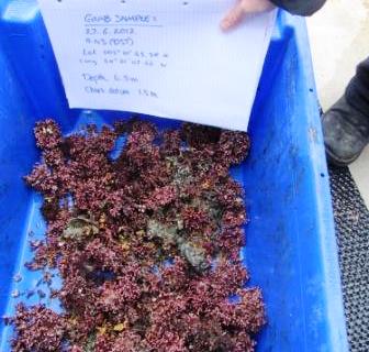
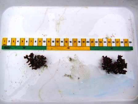
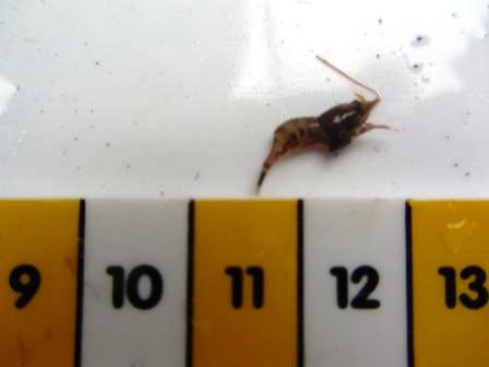
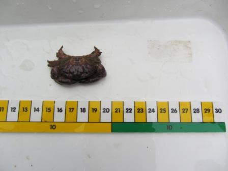
Figure 44 (top left) - maerl a protected calcareous algae.
Figure 45 (top middle) - Carodia spp.
Figure 46 (top right) - Cancer pagarus (Edible crab)
Figure 47 (bottom left) - an unidentified crab carrying eggs
Figure 48 (bottom middle) - Pinotheres Pisum (Pea crab)
Figure 49 (bottom right) - Galathea squamifera
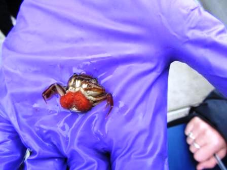
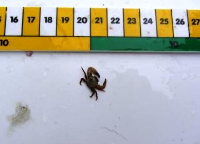
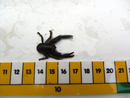
Discussion - (back to top of Geophysical Boatwork/webpage)
Findings from the Drop camera footage (figure 40-42) and Grab sample (figure 43), combined with features seen on the sidescan trace mosaic, indicate that there are still large beds of healthy maerl present within the Fal estuary. However areas surveyed by video around St Mawes showed signs of deterioration and discolouration, as seen in figure.., where the maerl has been turned white by death of symbiotic algae.
This correlates with findings of the report “Assessment of Maerl in the OSPAR area” (Hall-Spencer et al., 2007) which states that the quality of maerl beds in the UK has declined, largely due to the practice of dead maerl extraction for commercial use in things such as agricultural fertiliser. Dredging disturbs the seafloor, re-suspending plumes of sediment, which may be carried by currents and deposited as smothering layers over the maerl beds. This inhibits photosynthesis of the algae and leads to death of the maerl. The input of sewage into the estuary can have a similar smothering effect or may lead to increased turbidity in the overlying water column due to eutrophication. Changes in farming practices have also increased the turbidity of the estuary due to larger silt loads and higher nutrient run off (Birkett at al., 1998). As photosynthetic organisms, maerl rely on irradiance levels sufficient to support viable rates of photosynthesis. Increased turbidity will reduce the depth to which light can penetrate and potentially inhibit the maerls ability to photosynthesise. Anchor moorings of small vessels and heavy demersal fishing gear also have a directly damaging impact and are considered a serious problem, stripping patches of maerl and eelgrass beds (Birkett et al., 1998).
As such it is possible to infer that there will be a high possibility of detrimental impact for the maerl beds and habitats within the estuary if the proposed shipping channel were to be dredged in 2013. Such a large channel would suspend great amounts of sediment to smother the mearl beds and the subsequent increased shipping traffic would bring higher levels of anchor damage and water pollution.
Maerl bed habitats have a high benthic biodiversity and are home to a number of commercial viable species such a juvenile cod and broodstock bivalves (Hall-Spencer et al., 2007). They are also home to crustaceans, such as the edible crab, echinoderms, such as the brittle star, and the rare species Gobius couchi. Beds of eelgrass are important in providing shelter for anemones, seahorses and juvenile fish (1). Damage to these beds both direct and indirect would be devastating to the local ecosystem as habitat destruction would leave organisms vulnerable to higher rates of mortality.
It appears that the proposed dredging would have a significantly negative impact on the maerl beds, organisms already identified as areas of interest for conservation. It would be devastating to the associated organisms and ecosystems and as such it would be advised that the application be rejected pending further investigation of "down the line" effects of damage to the maerl beds.
References - (back to top of webpage)
Journal Publications
Anderson, D. M. (1998) Physiology and Bloom Dynamics of Toxic Alexandrium Species, with Emphasis on Life Cycle Transitions. Physiological Ecology of Harmful Algal Blooms, V. 41, I. 1, pages 29-48
Birkett, D.A., Maggs, C.A., & Dring, M.J. 1998. ‘Maerl: An overview of dynamic and sensitivity characteristics for conservation management of marine SACs.’ Scottish Association for Marine Science (UK Marine SACs Project). 5.
Fogg, G.E., Egon, B., Hoy, S., Lochte, K., Scrope-Howe, S. and Turley, C.K.M., (1985.) Biological studies in the vicinity of a shallow-sea tidal mixing front. 1.Physical and Chemical Background. Philosophical Transactions of the Royal Society of London. 310, 407-433.
Hall-Spencer, J.M., J. Kelly, C.A. Maggs. 2007. ‘Assessment of maerl beds in the OSPAR area and the development of a monitoring program’. OSPAR Comission Biodiversity Series.
Holligan, P. M. and Harbour, D. S., 1977, ‘The vertical distribution and succession of phytoplankton in the western English channel in 1975 and 1976’, Journal of the marine biological association of the United Kingdom, 57, 1075-1093.
Kiorboe, T. (1993). Turbulence, phytoplankton cell size, and the structure of pelagic food webs. Adv. Mar. Biol. 29, 1-72.
Maddock, L., Boalch, G. T. and Harbour, S., 1981, ‘Populations of phytoplankton in the western English Channel between 1964 and 1974’, Journal of the marine biological association of the United Kingdom, 565-583.
Milward, R. Grant, A. (Feburary 2000) Pollution-induced tolerance to copper of nematode communities in the severely contaminated restronguet creek and adjacent estuaries, Cornwall, United Kingdom. Environmental Toxicology and Chemistry, V. 19, I. 2, pages 454-461.
Pirrie, D. Power, M. R. Rollinson, G. Camm, S. G. Hughes, S. H. Butcher, A. R. Hughes, P. (June 2003) The spatial distribution and source of arsenic, copper, tin and zinc within the surface sediments of the Fal Estuary, Cornwall, UK. Sedimentology, V. 50, I. 3, pages 579-595.
Pritchard, D. W. (1967) What is an Estuary: Physical Viewpoint. Washington D.C : American Association for the Advancement of Science. Pages 3-5.
Southward, A.J., Langmead, O., Hardman-Mountford, N.J., Aiken, J., Boalch, G.T., Dando, P.R., Genner, M.J., Joint, I., Kendall, M., Halliday, N.C., Harris, R.P., Leaper, R., Mieszkowska, N., Pingree, R.D., Richardson, A.J., Sims, D.W., Smith, T., Walne, A.W. and Hawkins, S.J., 2005 'Long-term oceanographic and ecological research in the western English Channel'. Advances in Marine Biology, 47.
Vallet, C. and Dauvin, J.C., 1999, ‘Seasonal Changes of Macrozooplankton and Benthic Boundary Layer Macrofauna from the Bay of Saint-Brieuc (Western English Channel)', Journal of Plankton Research, 21, 1 35-49.
Wishner, K. Durbin, E. Durbin, A. Macaulay, M. Winn, H. Kenny, R. (November 1988) Copepod Patches and Right Whales in the Great South Channel off New England. Bulletin of Marine Science, V. 43, I. 3, pages 825-844.
Web References
48003 - Fal at Tregony. (n.d.). Retrieved July 06, 2012, from The Centre for Ecology and Hydrology: http://www.ceh.ac.uk/data/nrfa/data/time_series.html?48003
Cornwall Council. 2011. Meadows and Maerl. [Online] Available: http://assets.wwf.org.uk/downloads/mhcr.pdf [accessed 2012, 30th June]
http://www.westernchannel observatory.org.uk/l4_zooplankton.php