Falmouth 2012

Group 11

Group

Alex Hewitt

Cecilia Roos

Foivi Kouraki

Sally Stewart-Moore

Sam Leach

Sian Crowley

Robin Rigby

Roisin Quinn

Location

The Fal estuary (Figure 1.1) is the largest estuary in the UK, and the deepest in Europe (Pirrie et al 1995). It is a drowned river valley (ria) with a 127km shoreline, extending from the entrance (between Pendennis Point and St Anthony Head) 18km inland to the northern most tidal limit at Tresillian. It can be divided into two sections; the inner tidal tributaries and the outer tidal basin, known as the Carrick Roads which are characterised by a deep, narrow channel which ranges from 34m deep in the southern section to 5m in the River Fal (the northern section). The estuary is macrotidal at Falmouth with maximum spring tides of 5.3m and has a decreasing tidal amplitude towards Truro where maximum spring tides are 3.5m.

The Fal estuary system supports a diverse range of marine and coastal communities in a variety of habitats which include rocky shores, kelp forests, maerl (Phymatolithon calcareum, Lithothamnion caralloides) and eelgrass (Zostera marina) beds, saltmarshes and intertidal mudflats which make it an important conservation area. As a result the Fal has been designated as a Special Area of Conservation (SAC) under the European habitats directive.

Despite its SAC status, the Fal is regarded as one of the most polluted estuaries in the area, and this is mainly attributed to a long history of metal mining in southwest Cornwall, dating back to the Bronze Age. Mining was most intense during the industrial revolution, before declining towards the end of the 19th century. Despite the closure of the last mine in 1991, heavy metals have continued to enter the Carnon River through mine adits and spoil heaps, and as a result, a marked gradient of sediment metal concentrations have built up (Somerfield et al., 1994). The estuary is also subject to pollution pressures from other sources including sewage discharge, Tributyl Tin (TBT) and synthetic organic compounds.

The Fal is heavily exploited by maritime industry and leisure, and thus is of vital commercial and cultural importance on both a local and national scale. Therefore the collection of long term, comprehensive data on the physical, chemical and biological characteristics of the estuary are paramount to ensuring the development of effective management strategies in future.
 

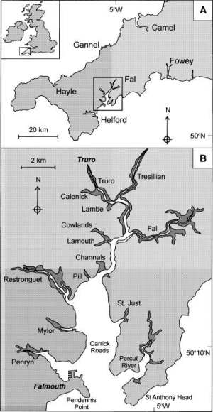Figure 1.1: The Fal estuary system, located in Cornwall, southwest England.

Estuarine

Boat Study

Introduction

 

Vessel	RV Bill Conway
Date	27/6/2012
Time	8:00-10:45 UTC
Cloud cover	8/8 nimbo stratus
Weather	Continuous light rain
Air temperature	14°C
High tide time (UTC)	10:20 (4.4 m)
Wind speed	2-4 kmph

The aim of our Fal estuary investigation was to study the spatial and temporal variations in stratification and to gain an understanding of the vertical and horizontal water column structure, the nutrient environment and the plankton community structure. Sample areas were chosen down the estuary (Figure 2.1) which provided insights into the physical, chemical and biological properties of the estuary. Temperature, salinity and light were measured to detect the physical properties of the estuary, while nutrient (dissolved silicate and phosphate) and dissolved oxyegn data provided an insight into the chemical properties of the estuary. Finally, the biological characteristics of the estuary were studied by measuring phytoplankton and zooplankton abundance.

In Situ Biological Methods

                 Table 1: Location of plankton net sampling

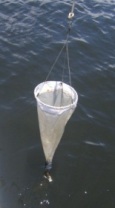
Plankton Net

Plankton samples were taken at stations 1, 2 and 3 representing the upper estuary and 4, 5 and 6 representing the lower estuary. Each sample was collected using a plankton net (Figure 2.2) connected to a 1 litre bottle towed at constant speed and depth behind the boat. A proportion from this bottle was removed at each station and added to Lugols iodine solution; a preservative of phytoplankton. To the remaining water sample formalin was added; a preservative of zooplankton. The flow through the net was calculated using an impellor coupled to a five digit counter. This allowed for the variability of flow rate and thus plankton counts between stations to be accounted for.

In Situ Physical Methods

Table 2: A table to show location, depths and start times of each station

CTD
The aim of using the Conductivity Temperature Depth Profiler (CTD) was to gather information on the structure of the water column through combining data from many different parameters.

The CTD was deployed at our chosen locations along the estuary (Table 2). It provided measurements of temperature, salinity, fluorometer and transmissometer readings whilst collecting water samples at desired depths using Niskin bottles.

Secchi Disk
This was used to measure depth of 1% irradiance and to give a representation of the euphotic zone depth at each station. Over the sampling period light levels and weather conditions remained similar. Several people helped in order to minimise human error.

ADCP

Table 3: A table to show the location, depths and start time of the ADCP transect at each station

An Acoustic Doppler Current Profiler (ADCP) was used to measure the water current speed and direction at specific station along the estuary (Table 3).

In situ chemical methods

Nutrients
Niskin bottles attached to a rosette were used at each station to collect samples throughout the water column. The samples were filtered on board to remove phytoplankton and zooplankton and subsequently stored.

Dissolved Oxygen
Samples were collected in the same way as nutrients. Two reagents were added to the samples; manganese chloride and alkaline iodine. The bottles were then sealed and submerged in seawater to prevent contamination.

Laboratory Methods/Analysis

The water samples were analysed for nutrients (dissolved silicon and phosphate) and dissolved oxygen. Phytoplankton and zooplankton were also identified and counted. Unfortunately our chlorophyll samples were lost in transit and thus fluorometer readings (from CTD) have been used instead.

Nutrients
The dissolved silicon content was determined using a method based on the techniques of Mullin and Riley (1955). The absorbance of the samples, blanks and standards were measured using a U1800 spectrometer at 810nm.

Dissolved phosphate content was determined according to the method by Parsons et al. (1984) and was measured using a U1800 spectrometer at 810nm.

Dissolved Oxygen
This was determined in accordance with the method described by Grasshoff et al. (1999).
 

Phytoplankton
Phytoplankton cell number per litre was estimated by counting individual cells under the microscope. The dominant phytoplankton taxa were identified.

Zooplankton

Zooplankton were analysed within a Bogorov chamber where abundance of each sample was recorded. Featured zooplankton included copepods, copepod nauplii, jellyfish larvae (cnidaria: hydrozoa), cirripedia, gastropod larvae and hydromedusa. Following this, the numbers recorded in each subsample were multiplied to provide an overall value of zooplankton abundance per metre cubed (Purdie, 2011).

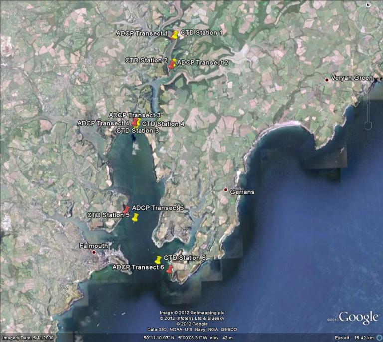
Figure 2.1: Map of CTD and ADCP station locations for the estuarine study

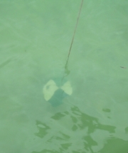
Figure 2.2: Phytoplankton net

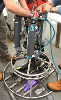
Figure 2.3: CTD

Figure 2.4: Secchi disk

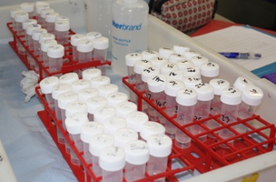
Figure 2.5: Samples bottles in the laboratory

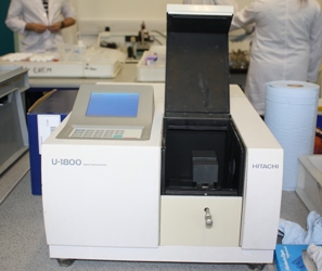
Figure 2.6: Spectrometer

Biological Results

A                                                                                              B                                                                                   C

                                                                        Figure 2.8

  D

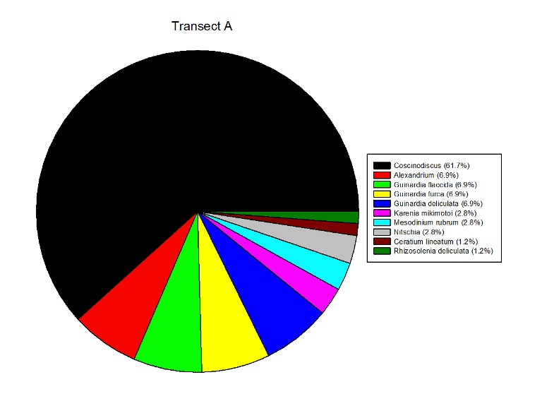
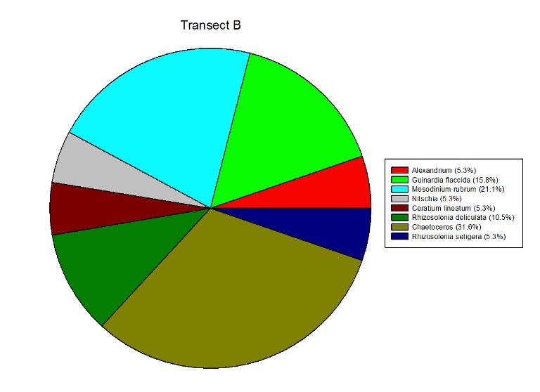
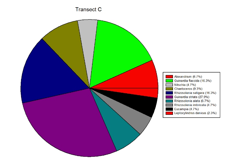
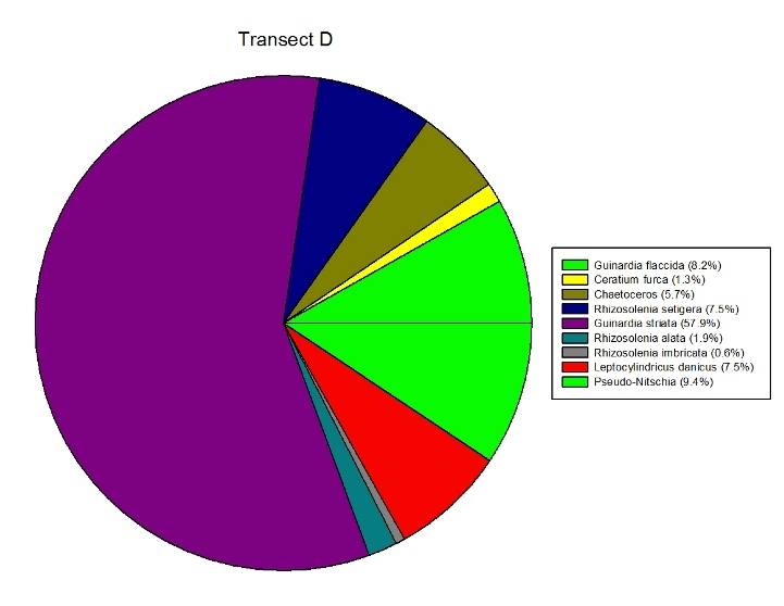
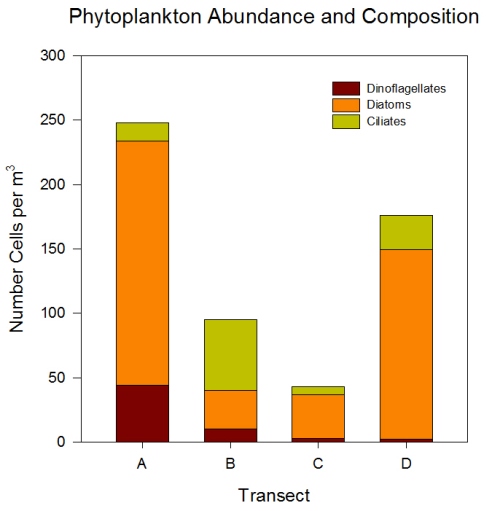
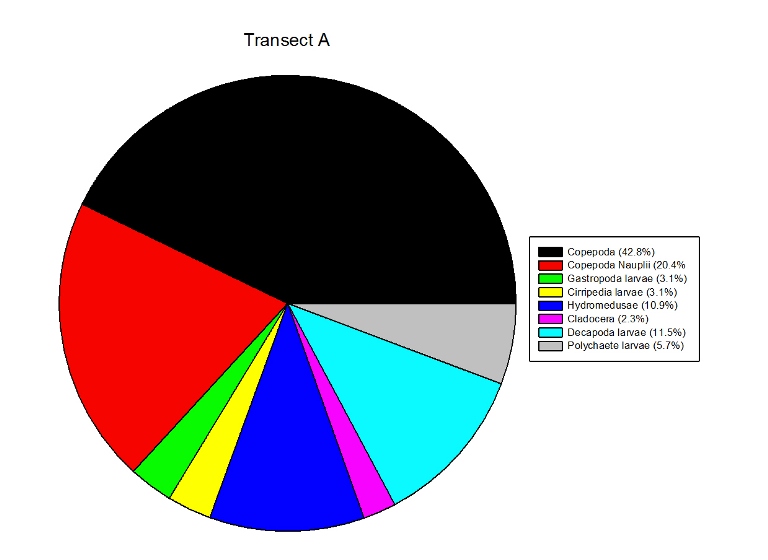
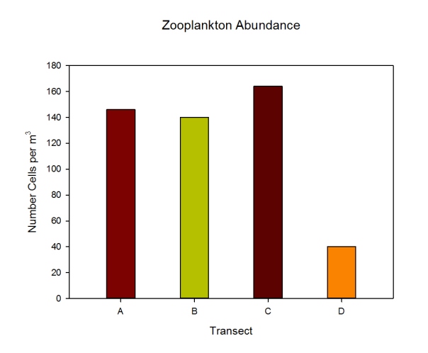
Figures 2.7 (A-D): These pie charts show the composition of the phytoplankton species collected in the samples from the estuary station transects

Figure 2.8: Bar chart showing number of cells per m³ of dinoflagellates, diatoms ciliates in transects A, B, C and D.

Phytoplankton

Figure 2.8 shows the phytoplankton counts for Transects A-D in the estuary, and the phytoplankton composition of each sample. Overall, there was a general decline in phytoplankton abundance in a seaward direction from Transect A (5745 cells per m3) to Transect D (683 cells per m3), with the exception of the Transect C sample which at 7655 cells per m3 is higher than Transect B (2451 cells per m3). Diatoms dominated the phytoplankton in the samples from Transects A,C & D, while the Transect B sample was dominated by ciliates. Dinoflagellates formed a significant proportion of the phytoplankton from Transect A, although dinoflagellate representation declined downstream from A-D.

The pie charts in Figure 2.7 show the relative composition of the phytoplankton from the water samples at Transects A-D. In Transect A, the phytoplankton was dominated by Coscinodiscus (Diatom) which accounted for 61.7% of the sample while the Transect B sample was dominated by Chaetoceros. Guinardia spp. (diatoms) formed a significant proportion of all the samples and were dominant in the samples from Transects C and D. Alexandrium was also relatively abundant in all the samples and Mesodinium rubrum formed a significant proportion of the phytoplankton in transect B.

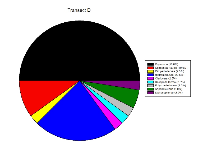
A                                                                                                 B                                                                                  C

                                              Figure 2.10

D

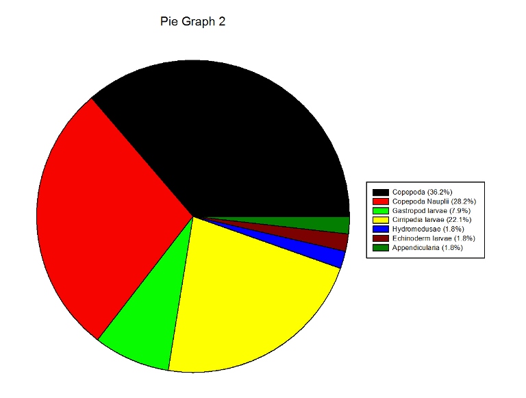
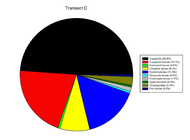
Figures 2.9 (a-d)- These pie charts show the composition of the Zooplankton species collected in the samples from the estuary station transects

Figure 2.10-Bar chart showing number of cells per m³ of zooplankton in transects A, B, C and D.

Zooplankton

Figure 2.9(a-d) illustrate the composition of the zooplankton collected in the samples from transects A,B,C & D. Copepoda were the dominant zooplankton in all 4 transects, closely followed by Copepoda Nauplii. Other abundant groups throughout the transects included Hydromedusae, Cirripedia larvae and Decapoda larvae.

Biological Discussion

Phytoplankton

The decline in phytoplankton abundance recorded with distance downstream can be attributed to a decline in nutrient concentration which ultimately limits growth. Furthermore, nutrient limitation is increasingly important during late Spring, when sampling occurred, due to nutrient depletion following the diatom spring bloom which occurs on an annual basis in temperate coastal waters (Sverdrup, 1953). This supports the evidence from Fig.2.8 which shows overall dominance by diatoms in the Fal estuary when sampling was carried out, while dinoflagellate abundance was relatively low, which indicates that diatoms tend to dominate the phytoplankton community during silicate sufficiency (Sommer, 1994). The decline in diatom dominance in a seawards direction may also reflect a decline in silicate concentration which diatoms have an ultimate growth requirement for (Tilman & Kilham, 1976). A long period of heavy rainfall prior to sampling may also be responsible for high phytoplankton abundance persisting for longer than normal.

Finally, the dominance of Chaetoceros and Guinardia spp. is consistent with other studies on the spring bloom in the waters of the western UK (Gowen et al., 1989).

Zooplankton
The results have shown that copepods dominated the zooplankton community throughout the estuary in late June. This can be attributed to timing; sampling occurred late in the diatom-dominated spring bloom which occurs in temperate coastal waters and is known to trigger an increase in copepod abundance (since they graze on the phytoplankton). This in turn provides an important food source for larvae and juvenile fish (Cushing, 1989). In this way, the significant proportion of larval zooplankton can be associated with the abundance of copepods and nauplii. Studies on the importance of copepod grazing on the spring phytoplankton bloom in the Western English Channel have reported temperature as a key factor determining the level of grazing since temperature ultimately controls the size of the copepod population by limiting ingestion rates and population development (Gowen et al., 1999). Therefore the size of the copepod population sampled in the Fal can be related to chlorophyll and temperature measurements.

Chemical Results

Nutrients/Chlorophyll vs Depth Estuary

Station 1

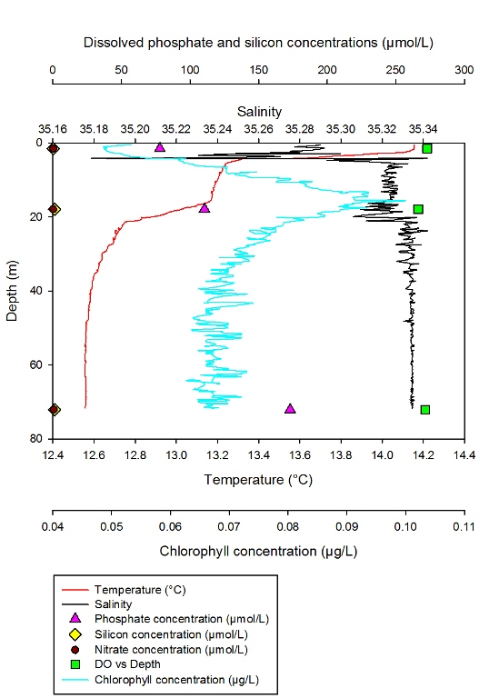
Description

Figure 2.11 Shows the changing concentrations of major nutrients and chlorophyll a with depth in the Fal estuary at station 1.

Dissolved phosphate concentration decreases from 444µmol/L in the surface waters to a minimum of 284µmol/L at a depth of 5m. From 5 to 6m the dissolved phosphate concentration increases from the minimum of 284µmol/L to the maximum of 514µmol/L.

Dissolved silicon concentration decreases from 51µl in surface waters to a minimum of 15µmol/L at 5m. From 5 to 6m the dissolved silicon concentration increases from the minimum of 15µmol/L to the maximum of 52µmol/L.

Chlorophyll a concentration increases from a minimum of 0.19µg/L in the surface waters to a maximum of 0.43µg/L at 3m. From 3 to 4m there is a rapid decrease in concentration, from 0.43µg/L to 0.25µg/L at 4m. After 4m, rate of decrease of concentration slows down, reducing to 0.22µg/L at 6m.
 

Discussion

At station 1 high concentrations of phosphate are observed, due to low uptake from phytoplankton which can be seen from the low chlorophyll levels. The peak in chlorophyll corresponds to the minimum phosphate and dissolved silicon in the water column. High turbidity, centred around a null point of low flow in the estuary, may be contributing to the low concentrations of chlorophyll due to photoinhibition of phytoplankton growth and reproduction (Perianez, 2005; Garniera et al. 2010).

Station 2

Description

Figure 2.12 shows the changing concentrations of major nutrients and chlorophyll a with depth in the Fal estuary at station 2.

Dissolved phosphate concentration decreases from a maximum of 324µmol/L in the surface waters to a minimum of 184µmol/L at 3m. The concentration remains constant at 184µmol/L between 3 and 6m. After 6m, concentration starts to increase with depth. At 9m concentration has increased to 284µmol/L.

Dissolved silicon concentration remains low uniformly down the depth profile. A slight decrease can be seen in concentration with depth, from 27µmol/L in surface waters to 12µmol/L at 9m.
Chlorophyll a concentration also remains low uniformly down the depth profile. It increases slightly from 0.20µg/L in surface waters to 0.21µg/L at 3m. From 3m, concentration slowly decreases with depth, reducing to 0.19µg/L at 9m.

Discussion

At station 2 the concentration of phosphate begins to decrease, particularly in the mid water column, as the river water begins to mix with the phosphate-poor seawater. Chemical removal could also be contributing to the decrease in phosphate levels (Morris et al. 1981).

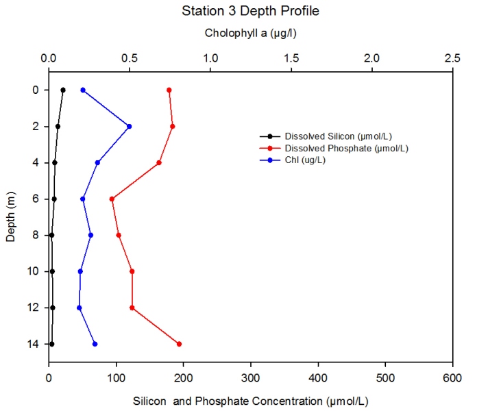
Station 3

Description

Figure 2.13 shows the changing concentrations of major nutrients and chlorophyll a with depth in the Fal estuary at station 3.- detailed depth profile.

Dissolved phosphate concentrations decreases slowly from 193µmol/L in the surface waters to a minimum of 94µmol/L at 6m. Below 6m a gradual increase of concentration with depth can be observed, reaching a maximum of 194µmol/L at 14m.

Dissolved silicon concentrations remain low uniformly down the depth profile. A slight decrease can be seen in concentration with depth, from 21µmol/L in surface waters to 5 µmol/L at 14m.

Chlorophyll concentration increases from a minimum of 0.21µg/L in the surface waters to a maximum of 0.50µg/L at 2m depth. From 2 to 6m there is a decrease in concentration, from 0.50µg/L to 0.21µg/L at 6m. Below 6m two small peaks in chlorophyll can be observed, one at 8m of 0.26 µg/L and the other at 14m of 0.29 µg/L
 

Discussion

In surface waters here phosphate concentration decreases by ~300µmol L-1 from station 1 to station 3. At station 3, as well as there again being increased mixing between river water and seawater, the effect of phytoplankton uptake of phosphate from the water column begins to become apparent, as chlorophyll levels increase to a maximum of around 0.5 µg l-1 in the surface 2m.

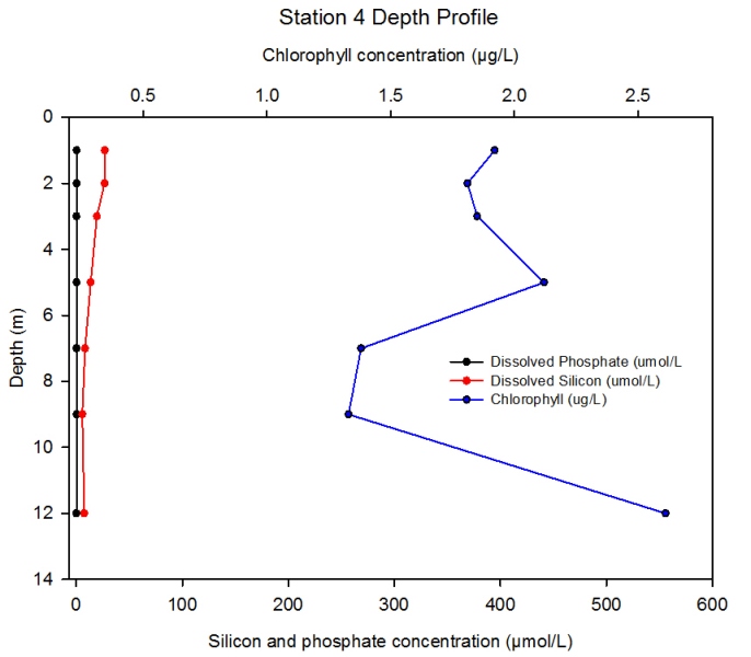
Station 4

Description

Figure 2.14 shows the changing concentrations of major nutrients and chlorophyll a with depth in the Fal estuary at station 4.- detailed depth profile: group 4 data.

Dissolved phosphate concentration remains extremely low uniformly down the depth profile. A slight decrease can be seen in concentration with depth, from 0.4µmol/L in surface waters to 0.2µmol/L at 12m.

Dissolved silicon concentrations decrease slowly from 26.9 µmol/L in the surface waters to a minimum of 5.8 µmol/L at 9m. From 9 to 12m there is a slight increase in concentration from 5.8 µmol/L to 7.6 µmol/L.

Chlorophyll concentrations increase slightly in the shallow waters, from 1.9µg/L in the surface waters to 2.1µg/L at 5m. From 5 to 7m concentration decreases from 2.1µg/L to 1.3µg/L. At 9m depth concentration rapidly increases with depth, from 1.3µg/L at 9m to 2.6µg/L at 12m.
 

Discussion

At station 4 the chlorophyll levels increase significantly throughout most of the water column. These high chlorophyll levels correspond with the low nutrient concentrations, due to uptake by phytoplankton. From 5 to 9m chlorophyll levels rapidly decrease, which could be due to zooplankton consumption. The water column becomes much more homogeneous with regards to phosphate concentration at station 4.

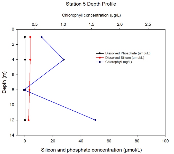
Station 5

Description

Figure 2.15 shows the changing concentrations of major nutrients and chlorophyll a with depth in the Fal estuary at station 5.- detailed depth profile: group 4 data.

Dissolved phosphate and dissolved silicon concentrations both remain low down the depth profile. Dissolved phosphate concentration increases slightly with depth from 0.09µmol/L in the surface waters to 0.14µmol/L at 12m.

Dissolved silicon concentration decreases slightly with depth from 3.9µmol/L in the surface waters to 2.7µmol/L at 12m.

Chlorophyll concentrations have two peaks down the water column. One at 4m depth, where it increases from 0.6µg/L in the surface waters to 1.0µg/L. The other is at 12m where it increases from a minimum of 0.3µg/L at 8m to a maximum of 1.6µg/L at 12m.

Discussion

Station 5 data shows an overall decrease in chlorophyll levels throughout the water column, but with a similar pattern of zooplankton grazing between 5 and 9m. There is also more pronounced evidence of zooplankton grazing in the top 2m. Chlorophyll levels may be lower overall due to a decrease in freshwater input with distance down the estuary. Phosphate levels remain very low, and dissolved silicon concentration also decreases to particularly low levels.

General Trends

As can be seen from Figures 1 (riverine end member) to 5(estuarine end member) the phosphate concentration gradually decreases with proximity to the sea. This is due to an increase in mixing between seaward-flowing river water, which contains high concentrations of phosphate, and landward-flowing seawater, which contains much lower phosphate concentrations. As phosphate decreases significantly, chlorophyll levels increase, suggesting that the phytoplankton are utilising the phosphate. Chemical processes within the estuary may also be contributing to this removal. Concentration of dissolved silicon also decreases slightly throughout the estuary for similar reasons (Bien et al. 1958).

Estuarine Mixing

Dissolved silicon vs. Salinity

Description

Since sampling was not done further up the estuary towards the riverine end, all data points are clustered towards the marine end member. The lowest salinity reading was 27.3 and the highest was taken to be the marine end member (36.0). Although all data points are within only a short distance from the theoretical dilution line (TDL) there are points both above and below the TDL with a greater weighting of points below the TDL. This indicates mild removal of dissolved silicon from the estuary and therefore non-conservative behaviour. Removal is most prevalent at salinities between 27.3 (51.5µmol/L) and 35.0 (2.7µmol/L) which were observed across all stations. Correlating this to phytoplankton abundance from the plankton net trawls shows a dominance of diatoms at all stations except B.
 

Discussion
The observed removal of dissolved silicon could be due to the occurrence of the spring phytoplankton bloom. This bloom is dominated by diatoms which require dissolved silicon for growth and frustule construction. The degree of removal is slight since: 1) sampling took place towards the end of the spring bloom and thus the abundance of diatoms is decreasing and 2) the area had experienced high volumes of rain water and thus run-off from land prior to and during the sampling period. This will have contributed dissolved silicon from rock weathering back into the waters (Cadee, 1978). This addition explains why the degree of dissolved silicon removal is less than would be expected at the time of sampling. Diatom presence was confirmed in the phytoplankton net samples.

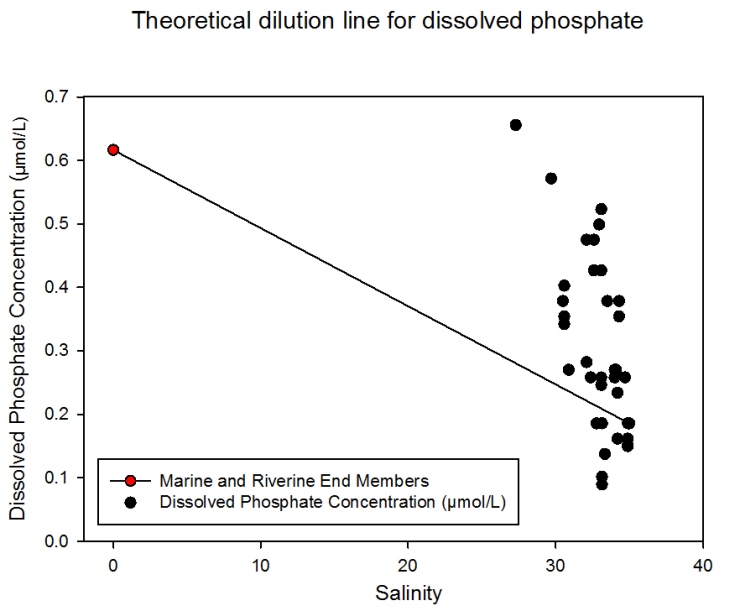
Phosphate vs. Salinity

Description

Again a wide range of salinity values towards the riverine end of the estuary were not sampled. Although all data points are based at the marine end member of the graph, they are widely varied in concentration values. The highest value (0.66 µmol/L) occurred at the most riverine sample (salinity 27.3) and the lowest value (0.09 µmol/L) at salinity 33.2. Overall a strong pattern of dissolved phosphate addition can be seen in waters of salinity range 27.3 to 35.0. However removal of phosphate can be seen at certain salinities (these include 33.2, 33.3, 34.2 and 34.9). The distance of data points above the TDL increases as salinity decreases indicating non-conservative behaviour.

Discussion

Dissolved phosphate is added to the estuary. The degree of addition increases with distance up the estuary (i.e. towards the riverine end). This addition, especially to the upper reaches, can be attributed primarily to run-off from the surrounding catchment area either directly or through groundwater flow. This is exacerbated by the fact that the freshwater catchment of the Fal lies in an extensive farming area where intensive fertiliser agriculture and sewage-treatment is practised (Langston et al., 2003). Furthermore the Fal catchment area has underlying impermeable bedrock which along with high rainfall experienced prior to and during the sampling periods contributes vast concentrations of phosphate into the estuary (seen in region of 27.3 and 35.0 salinity).

As pore waters are resuspended they add phosphate to the water column and further mixing results in higher phosphate concentrations in the water column (Mortimer et al. 1999). A possible cause of this is movement of large vessels through the estuary which disturb and re-suspend the sediment.

Physics

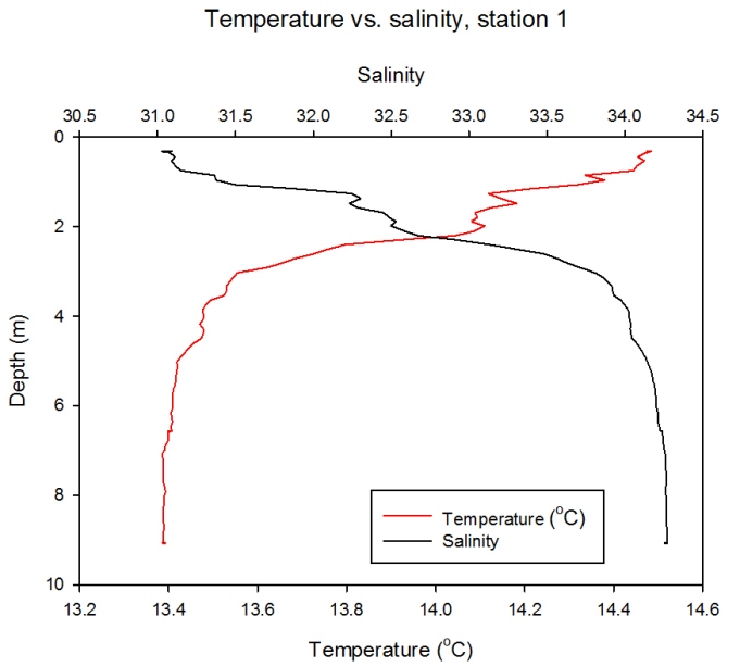
Salinity/temperature vs. Depth

Station 1

Description

Figure 2.18 shows that temperature undergoes a linear decrease from 14.5°C at the surface to 13.4°C at the maximum depth of 5m. Salinity shows an inverse relationship with temperature and undergoes a linear increase from a minimum 31 at the surface to a maximum of ~34 at 5m.

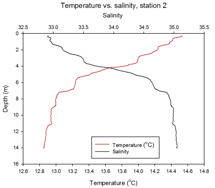
Station 2

Description

Figure 2.19 illustrates a roughly inverse relationship between temperature and salinity collected by the CTD. Temperature rapidly decreases from 14.6°C to 13°C and salinity increases from 33 to 35, between the surface and 8m depth. Salinity remains fairly homogenous beyond 8 m, and temperature also stabilises somewhat at the same depth, only decreasing by around 0.2°C between 8 and 14 m.

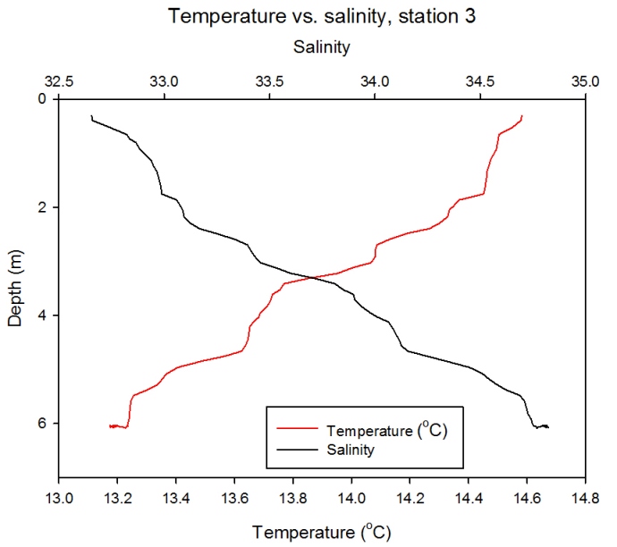
Station 3

Description
At station 3 (Figure 2.20),again there is an inverse relationship between salinity and temperature; salinity increases from around 32.6 at the surface to 34.8 at 6 m, and temperature decreases from 14.6°C to 13.2°C across the same depths. The salinity profile is fairly linear and there is no apparent halocline in the water column. The temperature profile shows a slight increase in the rate of change of temperature with depth below about 2 m.

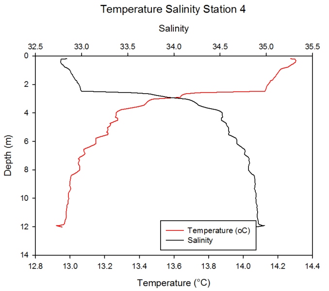
Station 4

Description

Figure 2.21 shows a temperature decrease as depth increases with surface temperatures of 14.3oC and temperature at the bottom of the water column (12m) falling to just below 12.0 oC. Greatest temperature decrease is seen between 2 and 4m depth, where temperature falls from 35oC to 33.3oC. As expected there is an increase in salinity with increasing depth; surface salinity of 32.8 and depth salinity just below 35.0 units. Greatest salinity flux is at similar depths to greatest temperature flux, with salinity increasing from 33.0 to 34.5 in approximately 1m of water. The graph shows an inverse relationship between salinity and temperature.
 

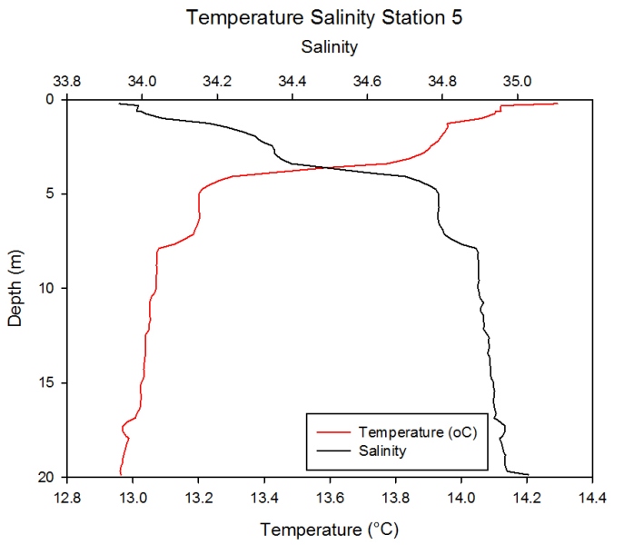
Station 5

Description

Figure 2.22 also shows an inverse relationship between temperature and salinity. The greatest fluxes are seen between 2 and 4m. Temperature levels at the surface are at 14.3oC and fall to just below 13.0oC with greatest decrease seen in the upper 3m of the water column. Salinity levels at the surface are 33.8 and increase with depth to 35.0 at 20 m.

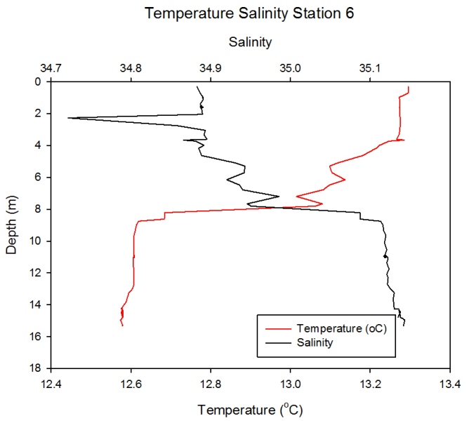
Station 6

Description

Figure 2.23 showed much more variation in salinity and temperature. Furthermore the greatest flux of salinity and temperature is lower in the water column at station 6 and occurs at approximately 8 meters depth. The temperature level at the surface is 13.3 and falls to 12.6 at depth. Salinity fluctuates a lot more than temperature and there is an area of particularly low salinity at 2 meters depth where salinity has dropped from 34.9 to 34.7 however it then rises again until it reaches over 35.1 at 15 meters depth. At station 6 in the lower estuary there is an area of low salinity at the top of the water column (2m) which is likely to be a freshwater pocket sitting above the saline water.

General Discussion

The general trend shown by the temperature salinity depth plots of the six stations shows temperature to decrease and salinity to increase with depth. The observed temperature decreases were due to solar radiation penetration which decreases with depth. Salinity increases with depth since saline water is denser than fresh water and thus sinks. Therefore the lighter freshwater flows out of the estuary above the denser saline water which flows into the estuary. This causes salinity stratification (halocline). A halocline can be seen in the upper section of the water column with the water below it being often homogenous or with just a small decrease in salinity. Across the 6 transects surface temperature remains fairly constant at around 14.5^oC. However surface salinity varies greatly; in the upper estuary salinity is low (around 31.0) due to the high freshwater inputs from the many tributaries whereas in the lower estuary it is much higher (34.81) due to the mixing of saline waters.

The Fal estuary is tidally dominated and impacted by freshwater inputs. Due to tidal mixing the change in temperature from surface to depth across the 6 stations is greater in the upper estuary, where mixing is less dominant, than in the lower estuary.

ADCP

Introduction

Richardson’s number
The Richardson number (Ri) is a dimensionless number used to describe the mixing which occurs in the water column; it is the ratio between density and shear stress with depth.
A Ri<1 is indicative of turbulent flow and a well-mixed water column. A Ri>1 is indicative of an absence of turbulence and laminar flow and thus a stratified water column. When 0.25<Ri<1 there is a gravitational shear and the water column becomes partially mixed. This can be calculated using the equation

where:

ρ2 is the density at the deepest point,
ρ1 is the density at the shallowest point,
ρ is the average density from two points,
h is the maximum depth from the CTD profile and
u is the average velocity from the ADCP profile.

 

All the Ri numbers are above 1 which suggests a stable and stratified water column. Station 3 (Ri= 7.00) has a well stratified and laminar water column. Samples at station 3 were taken an hour before high water which could explain this stability since at high water, water movement is reduced.

When describing water column flow several assumptions are made, and the points below need to be considered:
- Water layers move differently due to tidal influence and riverine input
- The CTD was deployed at different locations, to different depths and different times
- Weather conditions varied

Ri number was also calculated with depth for station 1 to show the changes through the water column. Although the Ri for station 1 shows an overall stable and laminar flow, when looking it with depth, turbulent layers can be seen. There is one exception at 1.89m where Ri= 0.37, indicating a stable layer with turbulent layers above and below it. A similar pattern to this was seen at other stations. When looking at the entire water column, it can be seen that turbulent flow exists with one or two laminar flow layers.

Residence time
Flow data were taken from CEH (Center of ecology and Hydrology) from the Fal at Tregony for a time period from 1978-2010. Although the Tregony tributary is quite far from the main body of the Fal estuary and is not the only riverine input, data from Kenwyn at Truro and Kennal at Ponsanooth (closer locations) were not available to download.

Mean Salinity (taken from all CTD data (stations 1-6)) =36.09
Sea salinity (taken from CTD data of station 4, average) =36.90
Total volume of estuary (taken from group 7/2011) =1.36*10⁷ m³
Riverine flux (data taken from CEH, 1978-2010) =1.03 m³/s

The average value for June from 1978-2010 was found to be 1.03m³/s. From the above calculation the residence time of the Fal estuary is approximately 3.32 days.
 

Discussion

General Discussion

Detailed description of results from stations 4 and 5 was not possible as there was a deep channel present half way through the transect making it impossible to collect measurements from the ADCP, therefore limited data were obtained.

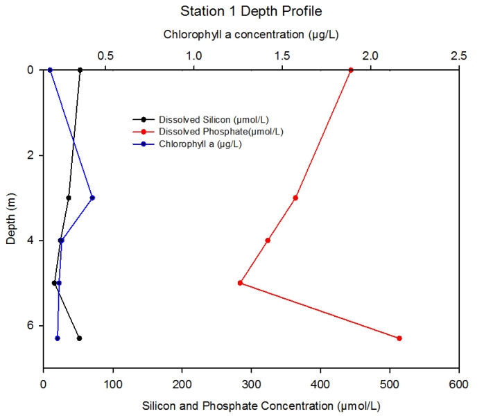Figure 2.11- Chlorophyll, silicon and phosphate concentration with depth at station 1

Figure 2.12- Chlorophyll, silicon and phosphate concentration with depth at station 2

Figure 2.13- Chlorophyll, silicon and phosphate concentration with depth at station 3

Figure 2.14- Chlorophyll, silicon and phosphate concentration with depth at station 4

Figure 2.15- Chlorophyll, silicon and phosphate concentration with depth at station 5

2.16- Estuarine mixing diagram for dissolved silicon

Figure 2.17- Estuarine mixing diagram for dissolved phosphate

Figure 2.18- Temperature vs. Salinity profile for station 1

Figure 2.19- Temperature vs. Salinity profile for station 2

Figure 2.20- Temperature vs. Salinity profile for station 3

Figure 2.21- Temperature vs. Salinity profile for station 4

Figure 2.22- Temperature vs. Salinity profile for station 5

Figure 2.23- Temperature vs. Salinity profile for station 6

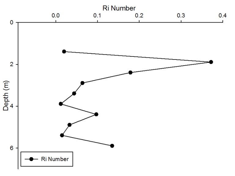
Figure 2.24: A depth profile to show how Ri number changes at station 1 though the water column.

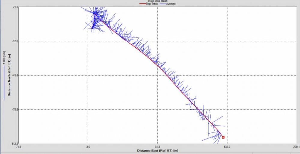
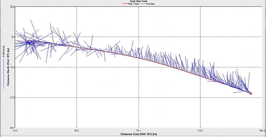
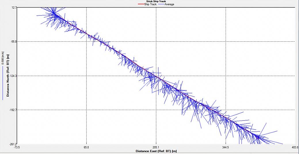
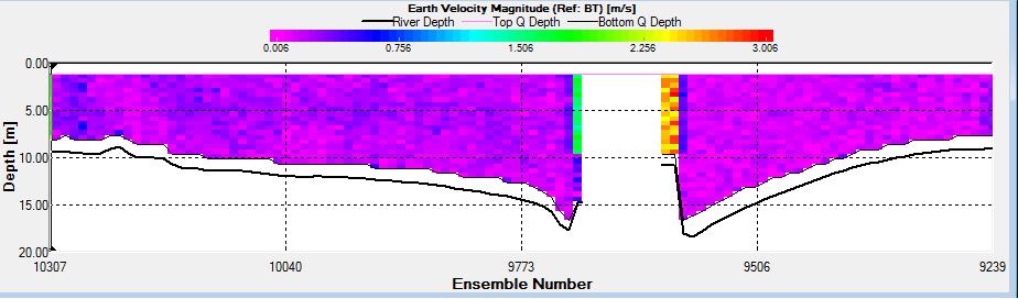
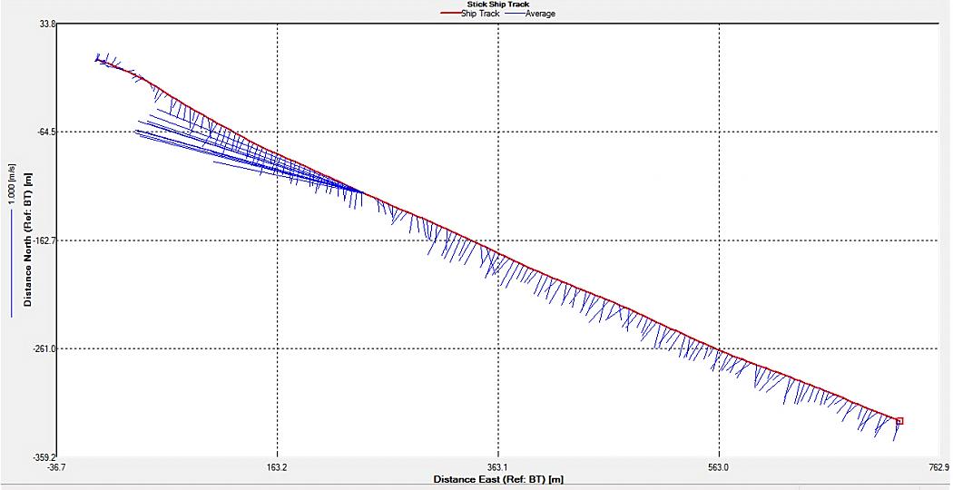
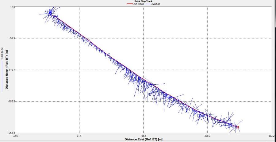
Figure 2.25: A ship stick track of the ADCP transect taken at station 1 at the top of the estuary (location 50° 14.390N, 05° 00.940W (at 08:32 UTC))

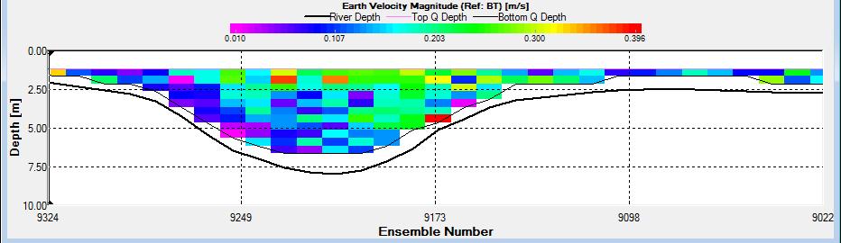
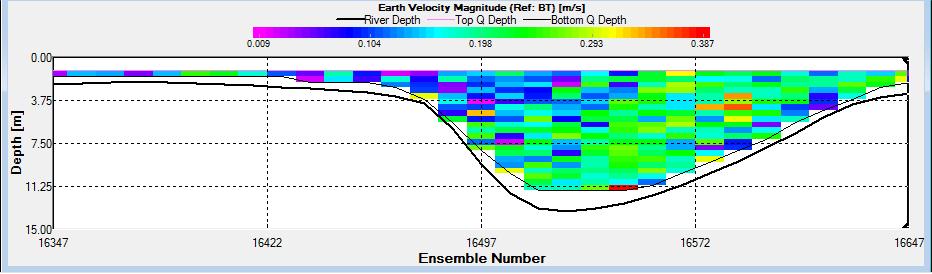
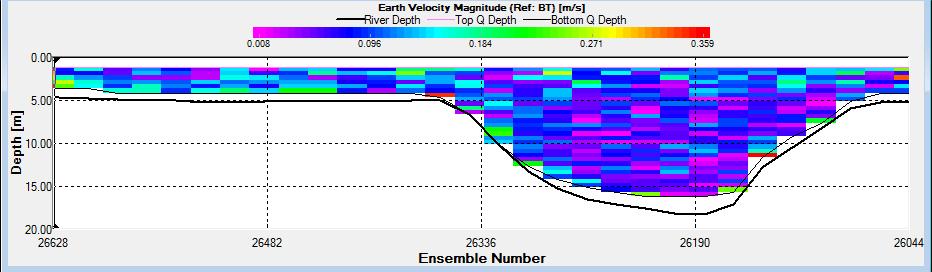
Figure 2.26: A velocity magnitude plot of the ADCP transect at station 1

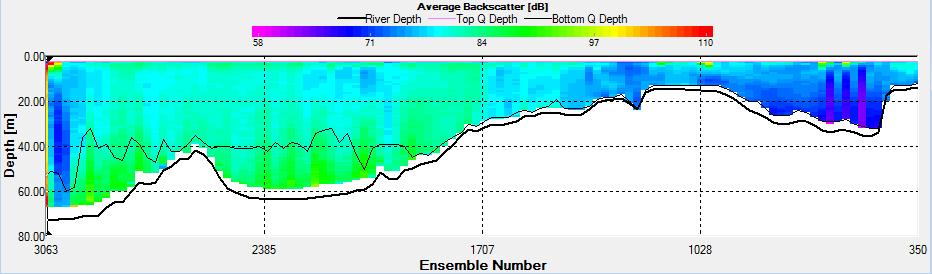
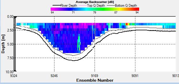
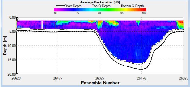
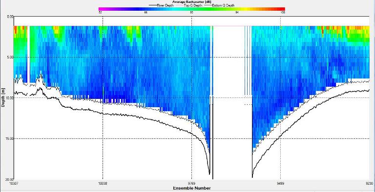
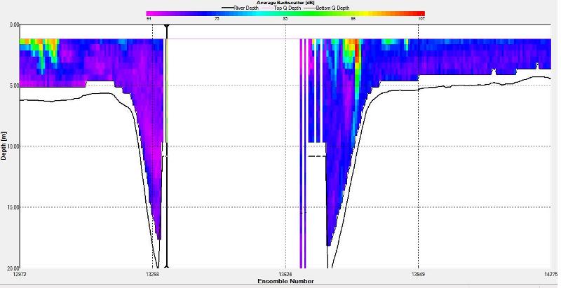
Figure 2.27: A backscatter plot of the ADCP transect at station 1

Station 1
Looking at the average ship stick track, there is great variation in the direction of surface water flow at the beginning of the transect (top left), however over most of the transect the flow is unidirectional (NE). At the end of the track the flow changes direction (SW).

Looking at the velocity magnitude plot it can be seen that the lowest velocities are at the start (up to 2m) and end of the transect at surface and deep waters. The velocity decreases gradually from the surface to deeper waters moving from the end towards the start of the transect. The low velocities at the end of the transect come from an increase in shear stress which was created due to the change in the flow direction (see ship track). The highest velocities (red and orange boxes) are found at 4.89m with 0.31m/s, 1.89m with 0.36m/s and 1.39m with 0.31m/s. The greatest horizontal velocity difference occurred at 1.89m, with a change from 0.37m/s to 0.15m/s, showing a 60.0% change in velocity. The greatest vertical change in velocity was found between 4.39m and 3.89m with 0.40m/s and 0.18m/s respectively, showing a change of 54.3%. The Vertical water column is more stable and thus less susceptible to turbulence due to the effect of gravity and other stabilising factors, such as salinity and density limit spontaneous turbulence as more energy is required for mixing.

Figure 2.27 shows the highest biological or sediment activity at the start of the transect in the surface waters; 1.39m with 94dB. High backscatter patches (with an average of 76dB) were found in the middle of the transect, from 3- 6m, and towards the end of the transect where the high shear stress was present.

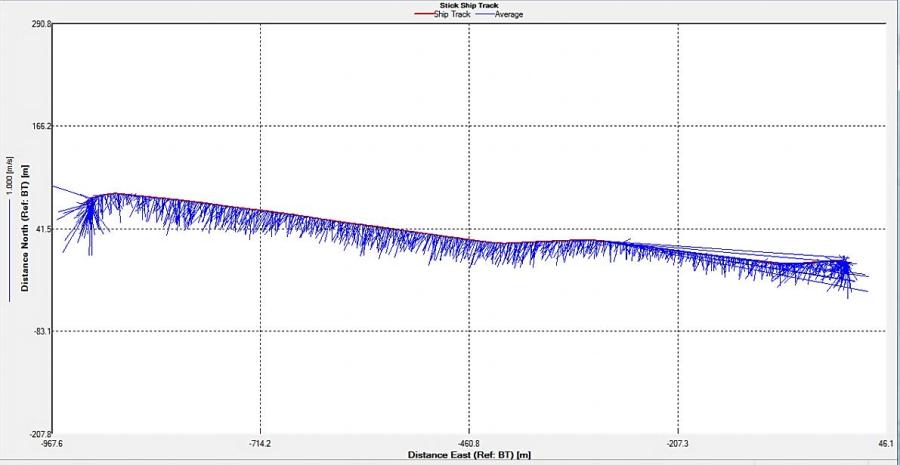
Figure 2.28 : The ship stick track for the ADCP at station 2 (location 50° 13.676N, 05° 01.030W at 09:27 UTC)

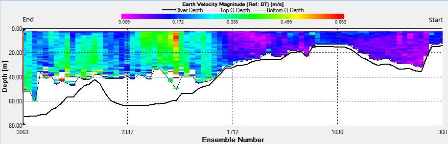
Figure 2.29: A velocity magnitude plot of the ADCP transect at station 2

Figure 2.30: A backscatter plot of the ADCP transect at station 2

Station 2
The flow is multidirectional at the beginning of the transect. Towards the middle of the journey it becomes unidirectional (N) and at the end it changes again and becomes multidirectional towards NS and SW.

The highest flow velocities were experienced at the middle and end of the transect, 0.39m/s at 11.39 m and an average of 0.35m/s around 4.39m. Towards the start of the transect flow velocities decreased. The greatest horizontal velocity change was seen at 4.89m with a 78.2% change (from 0.33m/s to 0.07m/s). The greatest vertical velocity change was observed between 4.89m and 5.39m, with 0.33m/s and 0.09m/s respectively, showing a 71.8% change.

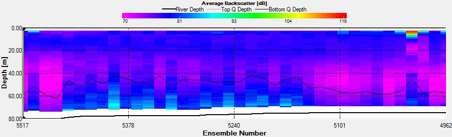
The backscatter does not show any distinct patterns meaning there was not significant biological or sedimentary activity. The only high values (100dB and 105dB) were seen at the beginning of the transect in surface waters (1.39m) where there was increased turbidity due to shear stress experienced in shallow water.

Figure 2.31 : The ship stick track for the ADCP at station 3 (location 50° 12.256 N, 05° 02.461 W, at 10:40 UTC)

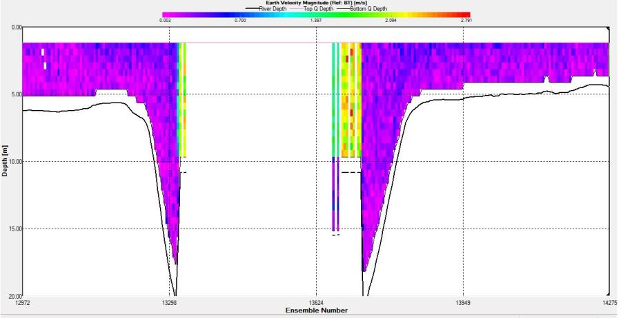
Figure 2.32: A velocity magnitude plot of the ADCP transect at station 3

Figure 2.33: A backscatter plot of the ADCP transect at station 3

Station 3

The flow is multidirectional throughout the whole transect with emphasis towards S and SW.

The velocity profile does not show any significant change in velocity. High velocities were seen at 11.39m (0.36m/s) at the start of the transect and towards the end of the transect at 4.39m (0.35m/s). The greatest horizontal change in velocity was found at 11.39m with a velocity change of 94.7% (from 0.36m/s to 0.02m/s). The greatest vertical change was observed between 4.39m and 3.89m; velocity change of 77.2% (from 0.35m/s to 0.08m/s).

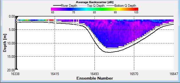
Figure 2.33 shows a distinct area of high backscatter (107dB) at the start of the transect in surface waters decreasing down to 4m. A second distinct zone of high backscatter is seen at the sea surface in the middle of the transect; this is indicative of high biological activity most likely due to the presence of phytoplankton and/or zooplankton populations.

Figure 2.34 : The ship stick track for the ADCP at station 4

Figure 2.35: A velocity magnitude plot of the ADCP transect at station 4

 3

Figure 2.36: A backscatter plot of the ADCP transect at station 4

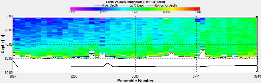
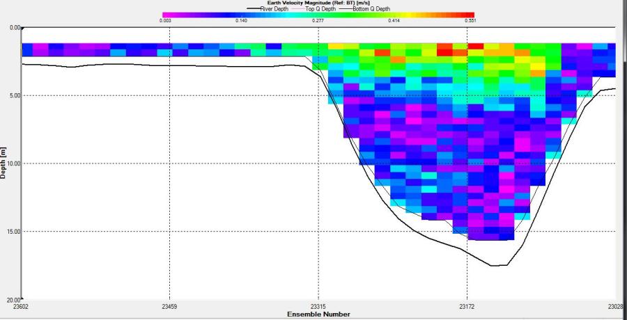
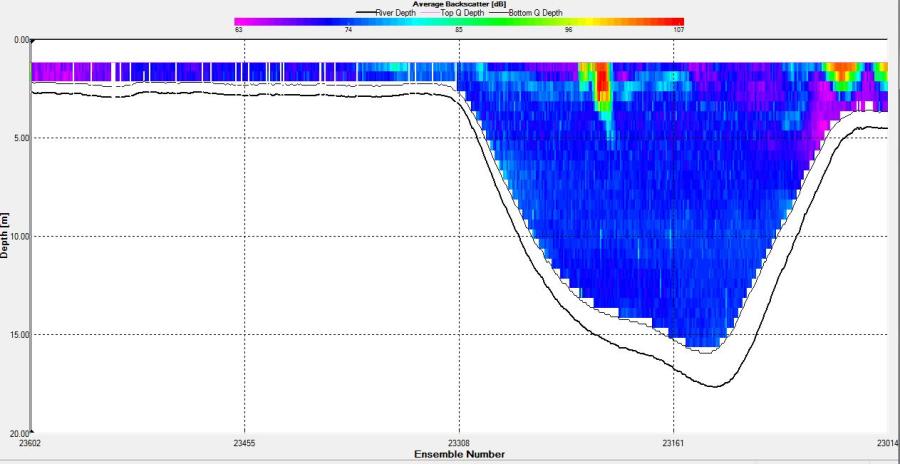
Station 4

The direction of the flow (SW) is fairly constant throughout the transect. Just before gap in the middle of the transect (the depth of the water was greater than the depth that ADCP could read) the flow velocity experienced a great increase which can be seen in the much longer lines on the ship stick track in an easterly direction. Velocity also increased on the other side of the gap seen in the velocity magnitude plot as green and blue vertical line (average flow velocity of 2.6m/s). At other parts of the transect there was an overall average velocity of 0.3m/s. The greatest horizontal and vertical changes in velocity could not be found since vast amounts of data were missing which would have led to a loss of accuracy.

Strong backscatter is seen at the sea surface almost throughout the entire transect. The first section at the start of the transect has an average backscatter of 100dB and the section after the gap has an average of 85dB. The sections at the end of the transect have an average of 90dB. The strong backscatter is evidence for some strong biological activity. This could be a possible result of phyto- and/or zooplankton population activity.

Figure 2.37 : The ship stick track for the ADCP at station 5

Figure 2.38: A velocity magnitude plot of the ADCP transect at station 5

Figure 2.39: A backscatter plot of the ADCP transect at station 5

Station 5

The flow shows similar structure to the previous station. It is unidirectional for the whole transect apart from the deep point where flow shows an enormous increase. The overall direction of the flow was SW but changed when the deep point was reached to NW.

The velocity profile is fairly constant as was seen at the previous station. High velocities were observed at both sides of the gap. The principle for horizontal and vertical change is the same as at the previous station.

Figure 2.40 : The ship stick track for the ADCP at station 6

Figure 2.41: A velocity magnitude plot of the ADCP transect at station 6

Figure 2.42: A backscatter plot of the ADCP transect at station 6

Station 6

Since this station was much shallower a full transect was able to be retrieved showing the separation of velocities from the surface waters within the channel and the bottom waters.

The flow is greatest in the surface waters of the channel (0.57m/s) and a minimum flow was seen at the bottom and sides of the channel (0.01m/s). Flow direction remains towards the mouth of the estuary since data was collected on the ebb tide. The flow is generally unidirectional (SW) throughout the first half of the transect. Over the second half spikes S and N moving away from the ship track are observed. At the sea surface the flow keeps the same direction showing laminar flow, however towards the deepest points, flow moves in varying directions indicating turbulence.

High velocities such as 0.57m/s are seen at the sea surface in the middle of the transect. At deeper layers the velocity is fairly constant with highest velocity (approximately 0.15m/s). The greatest horizontal velocity change was seen at 3.89m with 91.0% change (from 0.36m/s to 0.03m/s). The greatest vertical velocity change was observed between 3.39m and 3.89m, with a 76.45% change (from 0.31m/s to 0.07m/s).

Pontoon Study

Introduction

In order to determine whether variations in results between stations along the estuary were due to spatial or temporal changes over the tidal cycle, studies from a pontoon were made:
 

Date	29/06/2012
Time	13:45-17:45 UTC
Latitude	50°12.972N
Longitude	05°01.659W
Cloud Cover	6/8
Weather	Windy with occasional sun

The aim of the pontoon study was to gain an understanding of the temporal changes within the estuary over a tidal cycle. The water column was sampled every 15 minutes with data being recorded at 1m intervals. High tide occurred at 14:38 UTC (4.40m) which meant towards the end of the measurement time the water level dropped and measurements could only be taken down to 5m.

To analyse the depth profile over a tidal cycle data was collected using a YSI (multiparameter) probe, a current meter and a light probe. These allowed for temperature, salinity, pH, dissolved oxygen, current speed and direction of flow to be recorded. In addition chlorophyll data was obtained from a Niskin bottle every 1.0 hours at set distances; below the surface film and at maximum depth (5.0- 6.0m).

Physics

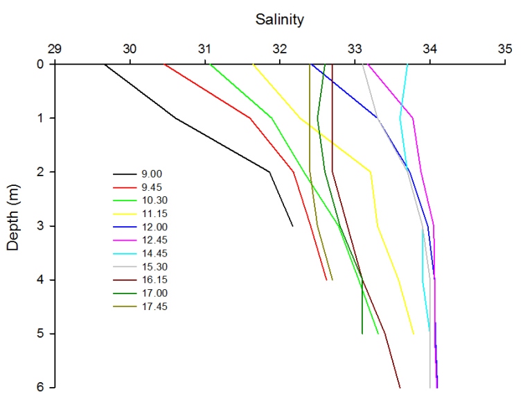
Salinity vs. Depth

Description

Figure 2.43 shows time series data of salinity measured every 15 minutes off a pontoon from 9:00 UTC up to and including 17:45 UTC. It can be seen that salinity increases by 0.1 - 0.5 salinity units every 15 minutes up until 12:45. After 12:45 salinity begins to decrease steadily as time continues.

At 12:45 the salinity reading was 33.2 at the surface and 34.1 at six metres. Over the remaining sampling period of 3:45 hours, surface salinities increased by 3.5 salinity units and by 2 salinity units at depth.

Discussion

The initial increase in salinity coincides with high tide at 12:38 UTC, thus following the increase in marine water up into the estuary. The salinity decreases with time after high tide as the riverine water flows past the pontoon and out to sea. This is seen particularly clearly at the time closest to low water (9:00 UTC) which gave the lowest salinity value (surface 29.7 and three metres 32.2). Overall, there is a gradual increase (before high tide) followed by gradual decrease (after high tide) in salinity over time.

Flow Rate

Description
Figure 2.44 shows the change in flow rates with depth at the pontoon over the tidal cycle. The greatest flow rate (0.97m/s2) was recorded at 12:20 at 1m and increased again slightly to 0.34m/s2 at 4m. High flow rates were also recorded at 11:20, with peaks in flow at 2m and maximum flow of 0.6ms2 at 4m. Lower flow rates were recorded at 14:45 and 15:45 and were more uniform throughout the water column. Flow rates increased at 16:45 and again at 17:45, whilst remaining relatively uniform throughout the water column. The majority of the depth profiles at the pontoon showed decreasing rates of flow at the bottom of the water column (between 5 and 6m).

Discussion
The results for the depth profiles of flow rates at the pontoon are ultimately attributable to tidal flow in the estuary as maximum flow rates were recorded at 12:20 shortly before high water (12:38). This flood tide is responsible for the shear flow observed in the upper water column (1m). Prior to high water, flow rates declined, and were lowest from 14:45 to 15:45 due to the slower ebb tide. An increase in this ebb flow however can be attributed to the increased flow recorded later on after 16:45. The uniformity of the flow rates throughout the water column at 16:45 and 17:45

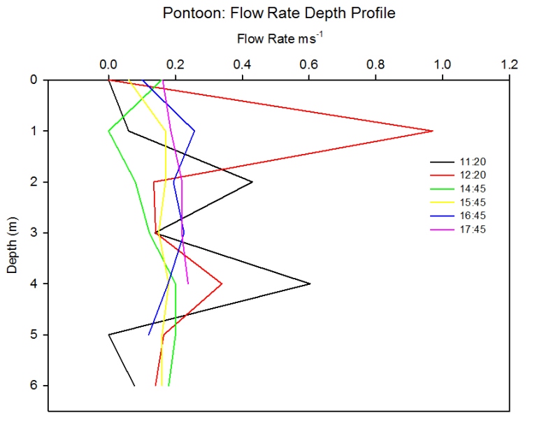
The decline in flow rates throughout the depth profiles result from friction with the estuary bed, disrupting flow and causing turbulence.

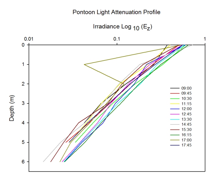
Light Attenuation

Description
Figure 2.45 shows the change in light attenuation over the tidal cycle at the pontoon. All the light profiles follow the same general pattern with an exponential decline in irradiance with increasing depth. With the exception of the 17:00 sample, all the attenuation profiles followed the same profile and declined at a steady rate through the water column. At 17:00 an decrease in irradiance was recorded at 1m, before increasing again at 2m.
 

Discussion
The exponential decline in light with depth is typical of light attenuation in the water column which is affected by 2 processes; absorption and scattering. While absorption removes light altogether, scattering changes the direction of propagation. This attenuation of light is caused by the water itself and dissolved particulate substances such as dissolved organic matter and suspended particulate matter. Therefore in estuarine water where freshwater input is high and therefore dissolved particulate matter is high, light attenuation will be increased and light penetration is limited and this ultimately restricts production by photosynthetic organisms. Tidal flow will influence the amount of particulate and dissolved matter in the water column, and therefore can be expected to have an effect on light penetration in the water column, although in this case there is no clear pattern evident over the tidal cycle. The increase in irradiance at 1m in the 17:00 profile can be attributed to experimental error, as it is not possible for light to be produced in the water column.

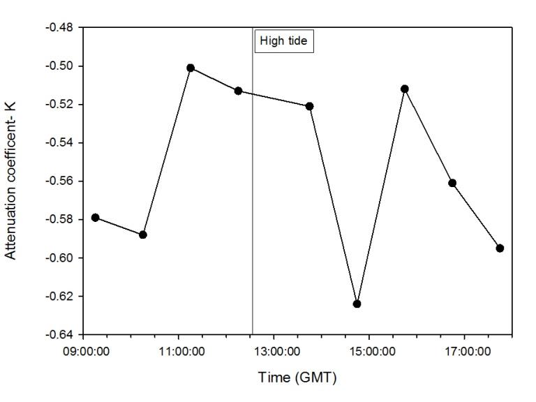
Light Attenuation Coefficient (K)

In order to visualise how much suspended matter was being mixed throughout the water column along a time scale of a tidal cycle, the attenuation coefficient, K, was calculated and plotted on a time scale graph.

Description
The attenuation coefficient, k, varies greatly over the tidal cycle. K increases from -0.59 at 10:15 to a maximum peak of -0.50 at 11.50. From 13:15 to 14:45 a rapid decrease in K can be observed, from -0.521 to a minimum of -0.624. K increases rapidly again from -0.624 at 14:45 to -0.512 at 15:45. From 15:45 until 17:45 K gradually decreases.

Discussion
At the point of change from flood to ebb tide, large tidal currents cause greater mixing and turbulence within the estuary. This causes sediments to be mixed up into the water column, making it cloudy and therefore reducing the light attenuation coefficient, k. This change from flood to ebb tide occurs after high tide. High tide, as marked on Figure? is at 12.30 UTC. Due to the time lag of tidal currents moving up the estuary, this change from flood to ebb tide will effect this location in the upper estuary a few hours later. This can be seen as the K minimum at 14:45.

Chemistry

Dissolved Oxygen Time Series
 

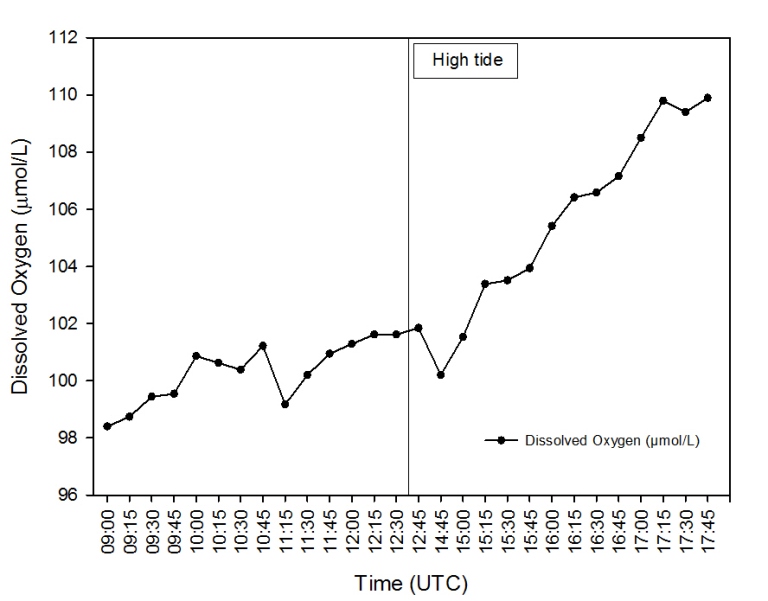
Description

Figure 2.47 shows the change in Dissolved Oxygen measured over the tidal cycle from 09:00 – 17:45 (UTC) on the Pontoon. Throughout the sampling period, the concentration of dissolved oxygen showed an overall increase. Prior to high tide at 12:38 UTC, the concentration of dissolved O₂ showed some fluctuations but increased gradually. No data was recorded immediately after high tide, and when sampling resumed at 14:45 there had been a marked decrease in dissolved O₂. After 14:45, the concentration of dissolved O₂ showed a steep and steady increase from 100.2µmol/l to 109.9µmol/l when sampling concluded at 17:45.  

Discussion

The results demonstrated an increase in dissolved oxygen concentration over time at the pontoon, with a sharper increase following high water. This change in dissolved oxygen can be associated with the increase in chlorophyll during the ebb tide caused by freshwater run-off, which leads to an increase in primary production by phytoplankton and thus an increase O₂ production.  Dissolved oxygen concentration is lower during the flood tide due to the progression up the estuary of sea water from the lower estuary which is depleted of oxygen.

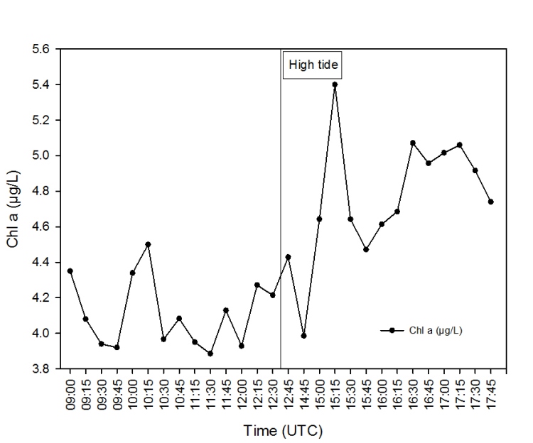
Chlorophyll a Time Series

Description
Figure 2.48 shows fluctuating data over the time period. Despite these fluctuations a general trend of increasing chlorophyll a from 09:00 UTC (4.35µg/L) up to and including 16:30 UTC (5.07µg/L) can be seen. Towards the end of the time period (after 16:30) a slight decrease in chlorophyll a concentration is seen (from 5.07µg/L to 4.73µg/L). At 09:00 the chlorophyll a measurement is initially high and then drops off before forming the increasing chlorophyll a trend. Anomalies can be seen at 10:15 (4.50µg/L) and 15:15 (5.40µg/L) which are much higher than the data points on either side of them.

Discussion

The chlorophyll a concentrations increase with time as high tide is approached. Chlorophyll a concentration is usually inversely correlated with tide stage when inverse correlations occur between chlorophyll a and salinity (Welch and Isaac, 1967).

The concentrations continues to increase after high tide as riverine water from upriver brings down nutrient-rich water from the tributaries which drain fertiliser-using agricultural land. This run-off is rich in phosphate and nitrate allowing rapid growth of phytoplankton and thus chlorophyll a.

Figure 2.43: A time series line graph to show how salinity varies with depth over time at a Pontoon located at 50°12.972N 05°01.659W.

Figure 2.44: Line plot showing the change in flow rates with depth at the pontoon. Line colour represents time (UTC) of sampling.

Figure 2.45: Line plot of the attenuation of light (Log10) in the water column over depth(m) measured at the pontoon. Line colour represents time of sampling (UTC).

Figure 2.46: Line graph illustrating the change in attenuation coefficient, k, over time on the pontoon.

Figure 2.47: Line graph illustrating the change in Dissolved Oxygen (µmol/l) over time on the Pontoon.

Figure 2.48: A time series line graph to show how chlorophyll a concentrations vary at a Pontoon located at 50°12.972N 05°01.659W.

Estuary Conclusion

An overall transition from well mixed at the mouth of the estuary to partially mixed waters at the riverine end is indicative of high tidal mixing towards the mouth of the estuary. Mixing in the Fal estuary is due to several reasons; semi diurnal mesotidal forces, the neap/spring cycle and topography of the estuary which ultimately determines much of the nature of the flow within it. Flow in the Fal estuary is dominated by tidal forcing; the flood tide being stronger than the ebb tide. Transformation from ebb to flood tide is shown well on the ADCP ship track plots and reinforced by Richardson number calculations. Another mixing force is the riverine flow from the upper estuary out to sea. A salt wedge towards the upper end of the estuary is present with reduced salinity on top due to freshwater inputs from upstream tributaries. A decrease in nutrients down the estuary as mixing with the saline sea waters dilutes the nutrients from the riverine water is seen. Greater phytoplankton populations are supported at the top of the estuary and appear to in turn support greater zooplankton populations here too. A decrease in salinity leads to a decrease in zooplankton as well.

The pontoon data showed a gradual increase with time in dissolved oxygen and chlorophyll a. A possible explanation for this increase is that the fresh water inputs of higher nutrients and dissolved oxygen are moved down the estuary on the ebb tide. Phytoplankton moved with the nutrients thus causing the increase in chlorophyll a over time at the pontoon. Irradiance decreased exponentially with depth which was expected.

Both dissolved phosphate and silicon show non-conservative behaviour. Phosphate shows addition throughout the estuary from agricultural inputs from surrounding farmland and numerous sewage works. Silicon undergoes slight removal possibly due to large amounts of diatoms in the upper and middle estuary. The main process controlling concentration is likely to be physical mixing as the majority of the points have plotted on or close to the TDL. A peak in chlorophyll corresponds with a minimum in dissolved phosphate and silicon.

Offshore

Introduction
 

The waters of the English Channel off Falmouth tend to be thermally stratified during the summer months and the strength of stratification is largely determined by a combination of water depth and tidal strength. However density structure, affected by freshwater inputs, wind strength and other climatic factors also influences stratification. As stratification stabilises the water column and thus affects vertical mixing, it has a profound effect on the physical and chemical properties of the surface layer of the ocean. In summer, surface waters in the English Channel tend to be nutrient depleted, while deep waters tend to be nutrient rich and therefore the rate at which growth limiting nutrients are mixed upwards in the thermocline is a key process determining biological productivity.

The primary aim of our offshore fieldwork was to determine how vertical mixing processes in the waters off Falmouth affect, directly and indirectly, the structure and functional properties of plankton communities. On the day of sampling, we aimed to locate the Frontal system offshore of the Fal estuary, created by the interaction between stratified and well mixed water masses and analyse its physical, chemical and biological characteristics.

Methods
 

Table 4: A table to show the locations, depths and sampling times of each sampling station

Sampling was carried out on R.V. Callista on the morning of the 5th June 2012. Taking weather conditions into account, a transect extending out from the Fal estuary towards Lizard Point was designated, along which sampling stations were located. In order to locate the frontal system, sea surface temperature was monitored along the transect, and stations were chosen where significant changes in SST were observed.

Physical Methods
CTD

The physical structure of the water column i.e. temperature and salinity at each station were measured using a CTD as for the estuarine sampling. Probes on the CTD Rosette system also measured turbidity, chlorophyll and irradiance.

Secchi Disk

Description can be found under the estuarine section of this website.

ADCP

The ADCP was intended to be used to describe the mixing regimes from the coastal to the offshore waters off Falmouth. The boundary at which the waters changed from coastal well mixed waters, to stratified offshore waters would give the location of the front. This would then allow for a more informed system of sampling either side of and at the boundary of the front. The ADCP profiler could also be used in a biological manner to locate the maxima of zooplankton due to the increase level of backscatter at this point.

Biological Methods
Plankton Net, Phytoplankton and Zooplankton
These were all done using the same methods as described in the estuarine section of this website with the exception of zooplankton samples. These were taken using a 200µm mesh vertical plankton net, which was deployed in the water column at depths corresponding to the water column structure or backscatter levels from the ADCP. These samples were then treated as described in the estuarine section of this website.

Chemical Methods
The analysis of the collected water samples (concentrations of dissolved silicon, phosphate and oxygen) took place on 06/07/2012 and the laboratory techniques were identical to those explained in the estuarine section of this website.
 

CTD and Nutrients Data

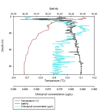
Station 1- (figure 3.2)

Description

In the upper 4m, temperature is constant with depth, remaining at approximately 13.1°C. From 4-6m temperature rapidly decreases from 13.1°C to 12.7°C and from 6-22m temperature gradually decreases from 12.7°C to 12.6°C. In the surface 4m, salinity is relatively constant with depth, remaining between 35.03-35.06. From 4-6m salinity rapidly increases from 35.05 to 35.15 and from 6-22m salinity gradually decreases from 35.15 to 35.19.

Chlorophyll concentration increases in the surface waters to reach a maximum peak of 0.974µgL-1 at 5m. From 5m it decreases with depth, reaching a minimum of 0.067µgL-1 between 12 and 17m. At 21m a small peak in chlorophyll concentration can be observed (0.085 µgL-1).

Dissolved phosphate concentration increases from 78µmolL-1at 4m to 158µmolL-1 at 15m while both dissolved silicon and nitrate concentration remain low down the water column, silicon at 2.7µmolL-1 and nitrate at 0.4µmolL-1. Finally, Dissolved oxygen concentration remains similar at both sample depths, 252µmolL-1 at 4m and 252µmolL-1 at 15m.

Discussion

At Station 1, the CTD profile for temperature and salinity can be attributed to the interaction of fresher, warmer estuarine water with cooler, more saline seawater at the mouth of the estuary. This profile may also have been enhanced by the ebbing tide at the time of sampling. This two-layered structure is typical of a partially mixed estuary in which tidal flow generates vertical mixing but is not strong enough to break down the difference in density between the two layers (Rockwell et al., 2000). The upper layer of less saline water may also be enhanced due to a period of high precipitation prior to sampling and there may also be a degree of surface warming from solar radiation, which is responsible for the higher temperatures at the surface.

The high chlorophyll levels in the upper layer of the water column, and especially at the base of the thermocline can be attributed to difference in density of the two layers, which inhibits vertical mixing. As a result of this coastal halocline the terrestrial nutrients and the phytoplankton which feed on them are maintained within the thin surface layer, thus leading to maximum chlorophyll at the surface (Menesguen & Hoch, 1997) where light penetration is sufficient for photosynthesis. The decline in chlorophyll with depth can therefore be attributed to a decline in light penetration due to attenuation by particulate and dissolved matter in the water column, which is enhanced by increased freshwater inputs. The decline in nutrients from the surface to depth is associated with the chlorophyll levels, as surface nutrients are depleted by phytoplankton utilisation. This can be seen for phosphate which increases with depth at Station 1. This also explains the slight decline in oxygen with depth, as primary production declines with diminishing light.


Station 2-(figure 3.3)

Description

In the upper water column, temperature decreases from 12.96°C to 12.79°C at 13m. From 13-30m temperature remains constant with depth, at 12.79°C before decreasing to 12.76°C where it remains throughout the rest of the water column. From 0-6m depth, salinity increases from a minimum of 35.31 to 35.34-35.35. From 6-65m depth salinity remains almost constant between 35.34 and 35.35, with the exception of peaks of lower salinity.

Chlorophyll concentration increases in the surface waters to reach a maximum of 0.086µgL-1 at 8m. From 8m, concentration decreases with depth, to 0.073µgL-1 at 32m. From 32-65m chlorophyll concentration remains between 0.073L-1 and 0.077L-1, with the exception of a large peak at 62m of 0.083µgL-1.

Discussion

The CTD depth profile for Station 2 represents a mixed water column, relative to the water column structure observed at Station 1. However there is a shallow fresher, warmer layer of water in the upper water column which is most likely a result of very high precipitation prior to sampling as well as solar energy warming the surface ocean. Below the upper few metres of the water column, salinity remains relatively uniform which indicates a significant amount of mixing. However temperature does decrease gradually with depth, and the notable decline in temperature at 30m may be due to wind mixing in the surface creating a layer of constant temperature down to the thermocline.

The low values for chlorophyll are attributed to nutrient depletion in the narrow surface layer of the water column, however due to mixing with the nutrient rich deep waters below, chlorophyll levels throughout the rest of the water column are relatively high as phytoplankton are able to utilise nutrients from mixing. Due to the more uniform density structure, vertical mixing also enables phytoplankton to maximise nutrient assimilation and photosynthesis. The high chlorophyll levels down to 20m and below are a result of this vertical mixing and increased light penetration which enable the phytoplankton to photosynthesise at greater depths (than in the estuary) while taking advantage of greater nutrient concentrations. The steady decline below 20m reflects the penetration of light, which decreases exponentially with depth in water.

Station 3(Figure- 3.4)

Description

From 0-10m, temperature decreases rapidly from 13.15°C to 12.86°C. Below 10m temperature decreases gradually with depth, reaching a minimum of 12.68°C at 55m and remaining at this temperature for the rest of the measured water column. In the surface 5m, salinity varies greatly from 35.34 to 35.30. Below the varying surface waters, salinity remains fairly uniform down the water column, remaining between 35.335 and 35.345
Chlorophyll concentration increases in the surface waters from 0.060µg/L to reach a maximum peak of 0.088µg/L at 16m. From 16 to 33m, concentration decreases with depth, to 0.072µg/L at 33m. From 33-65m chlorophyll concentration remains between 0.072 and 0.078, with the exception of two small peaks at 48m and 54m.
 

Discussion

Station 3 has a relatively similar water column structure to Station 2 in that there is a shallow surface layer with a low salinity and higher temperature, which again is most likely attributable to rainfall and solar radiation. Below this layer, the water column appears to be relatively well mixed although there is a gradual decrease in temperature and increase in salinity with depth. Chlorophyll also follows the same pattern as before, with very high levels between 10-20m. This results from a combination of sufficient light penetration for photosynthesis to occur with higher nutrient levels at depth. Chlorophyll levels decline slightly below 20m and remain uniform throughout the water column as phytoplankton benefit from vertical mixing which enables them to receive sufficient sunlight whilst benefitting from nutrient rich deep waters.

Station 4(figure 3.5)
 

Description

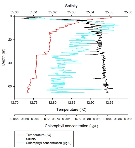
In the surface 5m, temperature decreases rapidly from 14.2°C to 13.3°C. A rapid decrease in temperature with depth can also be observed between 14m and 22m, where temperature decreases from 13.2°C to 12.7°C. From 43-72m temperature remains constant at 12.55°C. In the surface 5m, salinity varies greatly from 35.18 to 35.34. Below the varying surface waters, salinity remains fairly uniform down the water column, remaining between 35.30 and 35.34.
From 0-16m chlorophyll concentration gradually increases with depth, from 0.047µg/L to a maximum of 0.101µg/L at 16m. From 16-30m concentration gradually decreases with depth to 0.065µg/L at 30m From 30-72m concentration remains between 0.062µg/L and 0.075µg/L.
Dissolved phosphate concentration increases down the water column, from 78µmol/L at 1.5m, to 110µmol/L at 18m, to 173µmol/L at 72m while both dissolved silicon and nitrate concentration remain low down the water column, silicon at an average of 0.7µmol/L and Nitrate at an average of 0.5µmol/L. Finally, dissolved oxygen concentration remains similar down the water column, 272µmol/L at 1.5m, reaching a minimum of 266µmol/L at increasing to 271µmol/L at 72m.
 

Discussion

The CTD profile for Station 4 demonstrates a stratified water column which can be associated with the Frontal system we were searching for off Falmouth. This stratified water column is comprised of 3 layers; a surface layer of warmer, fresher water which again can be explained by freshwater input and solar radiation; a middle layer with a marked reduction in temperature and increase in salinity which are uniform down to 20m; and a lower layer from 20m downwards which is characterised by uniform high salinity, low temperatures and constant chlorophyll. This provides a suitable example of seasonal thermal stratification in the English Channel which creates a density gradient that inhibits vertical mixing.
In contrast to Station 1 in the estuary, maximum chlorophyll at Station 4 was recorded between 10-20m and this is due to the difference between thermal stratification in the open sea and thermohaline stratification in estuarine zones (Menesguen & Hoch 1997). While the coastal halocline maintains phytoplankton and the nutrients on which they feed in the surface layer, thermal stratification in the open sea, as seen at Station 4, prevents nutrients in the bottom layer from feeding phytoplankton in the surface layer. As a result the observed chlorophyll levels were lower in the stratified system at station 4 than at the mixed stations 2 & 3. At Station 4, the chlorophyll maximum was observed at approximately 20m at boundary of the upper layer, where light penetration is sufficient for photosynthesis and phytoplankton can maximise nutrient uptake as nutrient levels increased with depth.

Station 5

On return to the estuary, the CTD was also deployed at station 5 in the deeper section of the channel.  However the results from this profile represented a typical estuarine water column structure and therefore we chose not to analyse the data any further.

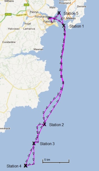Figure 3.1 : A map of the plan A route and sampling stations along the route

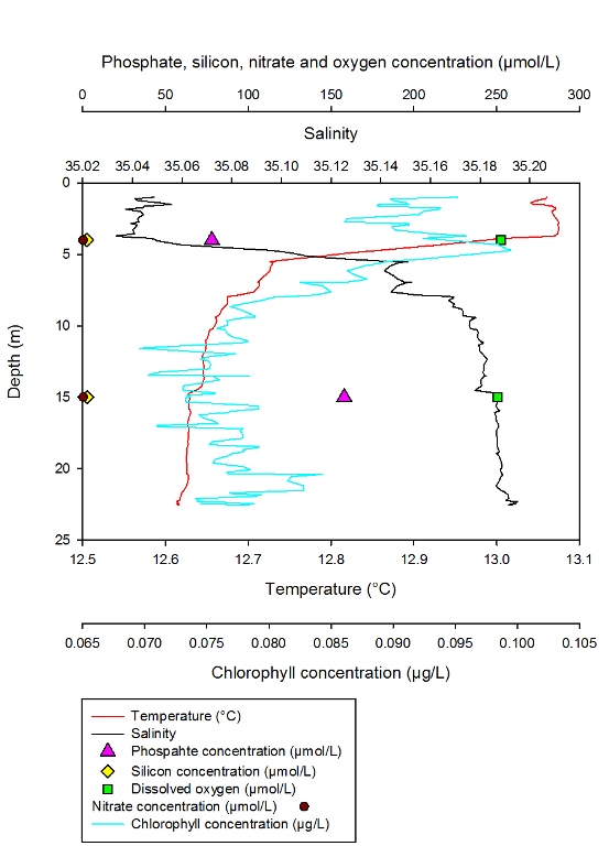
Figure 3.2: CTD profile for Station 1. Red line representing change in temperature (°C) with depth and black line representing change in Salinity with depth. Blue line corresponds to the change in Chlorophyll (µg/l) with depth. Data points also show nutrient and dissolved oxygen concentrations (µmol/l) throughout the water column.

Figure 3.3: CTD profile for Station 2. Red line represents Temperature (°C) and Black line represents Salinity. Blue line corresponds to Chlorophyll (µg/l).

Figure 3.4: CTD profile for Station 3. Red line represents Temperature (°C) and Black line represents Salinity. Blue line corresponds to Chlorophyll (µg/l).

Figure 3.5: CTD profile for Station 1. Red line representing change in temperature (°C) with depth and black line representing change in Salinity with depth. Blue line corresponds to the change in Chlorophyll (µg/l) with depth. Data points also show nutrient and dissolved oxygen concentrations (µmol/l) throughout the water column.

Phytoplankton

AB

Figure 3.6 (A & B): These pie charts show the composition of the phytoplankton species collected in the samples from the offshore station 1, depths 4.3 m (A) and 15.2 m (B).

Figure 3.7: These pie charts show the composition of the phytoplankton species collected in the samples from the offshore station 2, depth 31 m.

A                                                                                   B                                                                                        C

Figure 3.8 (A-C): These pie charts show the composition of the phytoplankton species collected in the samples from the offshore station 4, depth 1.5 m (A), 17.9 m (B), 72.1 m (C.

Description

Guinardia flaccida dominated the sample from 4.3m at Station 1 in the estuary, accounting for 70.8% of the sample. Other species identified included Rhizosolenia setigera (20.8%) and Rhizosolenia stolterfothii (8.3%). At 15.2m (Figure 3.6), the sample was more diverse and was dominated by R. setigera (27.9%), closely followed by R. stolterfothii (22.7%). Other abundant species included Chaetoceros (18.2%) and G. flaccida (13.6%).

At Station 2 (Figure 3.7) the sample from 31m was also dominated by G. flaccida which accounted for 24.3% of the sample. Thalassiosira rotula (18.9%) and other unidentified Thalassiosira species (18.9%) also contributed to a significant proportion of the sample, as well as Coscinodiscus (10.8%) and Pseudo-nitschia (10.8%).

At Station 4 (Figure 3.8) the 1.5m sample was also dominated by G. flaccida (31.2%), which was followed closely by Thallassiosira rotula (25.0%). R. setigera also formed a significant proportion of the sample, accounting for 18.8%, as well as Rhizosolenia alata which contriubted 15.6% of the sample. The sample from 17.9m was dominated by the species Leptocylindrus danicus which accounted for 48.3% of the sample. This was followed closely by Guinardia deliculata which formed 41.4%. Finally, at 72.1m, Chaetoceros and Karenia mikimotoi both formed a significant proportion of the sample, contributing 35.7% each.

Discussion

Copepoda dominated the zooplankton community at all the stations, which is typical for most cases. However, copepod dominance declined with distance offshore and other groups such as the Cladocera and Appendicularia became increasingly important. This transition in zooplankton community structure may be attributable to the frontal system located between stations 3 & 4, comprised of a thermally stratified water column in which phytoplankton are concentrated at the base of the euphotic zone. Therefore the zooplankton species observed in the deep sample may be grazing on the phytoplankton community above during the night time when they migrate vertically to the upper layer of the water column (Lampert, 1989).

Zooplankton

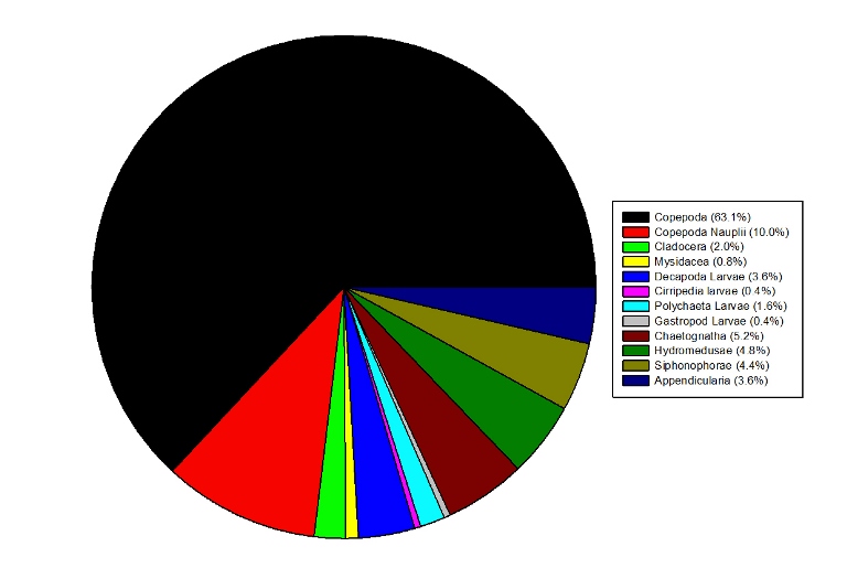
Figure 3.9: Pie Chart representing the percentage composition of the zooplankton sample collected at Station 2

AB

Figure 3.10: Pie Charts representing the percentage composition of the zooplankton sample collected at Station 4 at (a) 0-10m and (b) 10-27m.

Description

Copepoda dominated the zooplankton sample at Station 2, accounting for 63.1% of the sample, followed by Copepoda Naupilii which accounted for 10.0% of the sample.

In the surface layer at station 4 (0-10m), the zooplankton was also dominated by Copepoda (40.3%) and followed by Cladocera which accounted for 22.3% of the sample. Appendicularia and Siphonophorae also formed a significant portion of the sample.

Discussion

Copepoda dominated the zooplankton community at all the stations, which is typical for most cases. However, copepod dominance declined with distance offshore and other groups such as the Cladocera and Appendicularia became increasingly important. This transition in zooplankton community structure may be attributable to the frontal system located between stations 3 & 4, comprised of a thermally stratified water column in which phytoplankton are concentrated at the base of the euphotic zone. Therefore the zooplankton species observed in the deep sample may be grazing on the phytoplankton community above during the night time when they migrate vertically to the upper layer of the water column (Lampert, 1989).

ADCP

From the graphs we can see distinct patterns of thermocline along the water column.

At station 3, 1 weak and 2 strong thermoclines are apparent. The weak thermocline was observed at depths between 14m and 20m, the first strong thermocline between 30m and 36m and the second at 48m. The maximum Ri number for the weak stratification was 2.33 at 14m. The strong stratification had a Ri number of 35.5 at 32.5m for the first and 22 at 48m for the second.

At station 4 the same principle as for station 2 was applied due to the relatively high values of Ri.
The water column shows variable stratification. Mixed and stratified layers are apparent the whole way through the water column. A strong thermocline is apparent at 30m with Ri number of 52. Other small stratified layers were also present at 4m, 10m, 18m -20m and 42m. Mixed layers were present in between the stratified ones.

Several factors could have interfered with the accuracy of results for the calculation of the Ri number. As data were taken from both ADCP and CTD files, approximates of values were taken resulting in less accurate results.

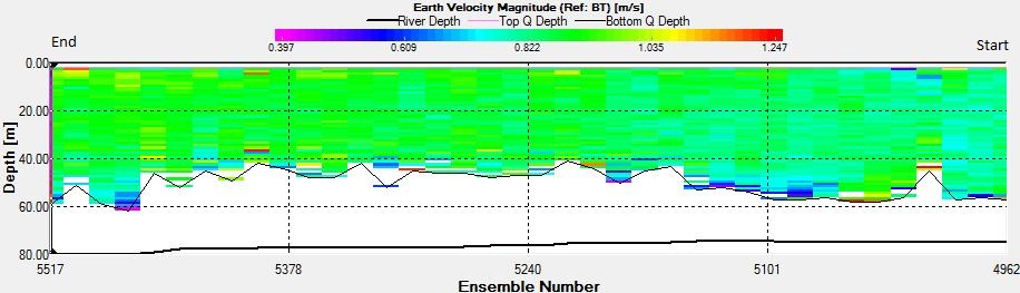
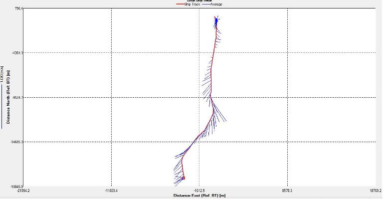Figure 3.11 : The ship stick track for the ADCP at station 1

Figure 3.12: A backscatter plot of the ADCP transect at station 4

Figure 3.13: A velocity magnitude plot of the ADCP transect at station 1

Station 1

At station 1 which was towards the estuary a distinct and strong thermocline from 4m to 6m can be seen; Ri number reached a maximum of 65, followed by mixed layers with Ri<1.

The strongly stratified layer was confirmed by the CTD graph, showing a thermocline and halocline at around 5m.

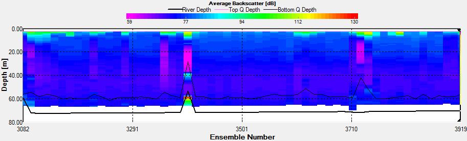Figure 3.14: A backscatter plot of the ADCP transect at station 4

Figure 3.15: A velocity magnitude plot of the ADCP transect at station 1

Station 2

At station 2, a logarithmic scale was used for the Ri number as it reached a value of 250. All the points at the right hand side of the depth line had Ri>1 and the ones on the left Ri<1; indicating layers of laminar and turbulent flow respectively.

A weak thermocline was created at 12m (Ri=6) followed by a mixed layer. Then again another thermocline is shown, much stronger from 16m to 24m.

The CTD graph, shows a small thermocline at 13m, confirming the weak thermocline on Ri graph, and another, stronger thermocline at around 30m. This agrees well with the Ri graph.
 

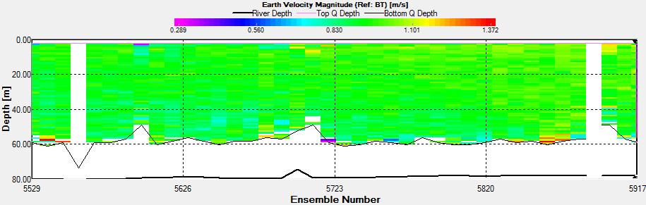
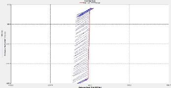Figure 3.16 : The ship stick track for the ADCP at station 3

Figure 3.17: A backscatter plot of the ADCP transect at station 4

Figure 3.18: A velocity magnitude plot of the ADCP transect at station 1

Station 3

At station 3, 1 weak and 2 strong thermoclines were apparent. The weak thermocline occurred between 14m and 20m, the first strong one between 30m and 36m and the second at 48m. The maximum Ri for the weak stratification was 2.33 at 14m and for the strong stratification was 35.5 at 32.5m for the first and 22 at 48m for the second.

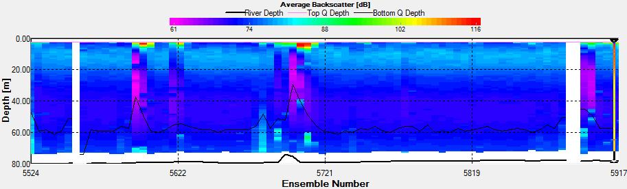Figure 3.19: A backscatter plot of the ADCP transect at station 4

Figure 3.20: A velocity magnitude plot of the ADCP transect at station 1

Station 4

At station 4 the same principle as for station 2 was applied due to relatively high values of Ri.

The water column shows variable stratification. Mixed and stratified layers are apparent the whole way through the water column. A strong thermocline is apparent at 30m depth with Ri= 52. Other small stratified layers were also present at 4m, 10m, 18m to 20m and 42m depth. Mixed layers existed in between the stratified ones.

The small thermocline at 20m can also be seen at the CTD graph, however, the strong stratified layer that is shown to appear at 30m it is not shown at CTD graphs.
 

Offshore Conclusion

The ultimate aim for the offshore study was to locate the frontal system offshore of the Fal estuary and analyse its physical, chemical and biological characteristics. From analysis of the CTD profiles at stations 1-4, we have been able to find the approximate location of the front between stations 3 and 4. As the CTD profile for Stations 2 & 3 were typical of a mixed water column, Station 4 further offshore demonstrated a stratified water column, which can therefore be associated with the Frontal System. Thus we can deduce from this that the frontal system met with the well mixed coastal waters approximately somewhere between stations 3  and 4 (Figure 3.1) on the day of sampling.


As stratification stabilises the water column, it has a significant effect on the physical and chemical properties of the ocean and therefore determines biological productivity. Therefore the position of this frontal system in relation to the coast, is an important factor affecting the dynamics and distribution of phytoplankton in the area, which in turn influences the distribution of zooplankton and thus has a wider influence on the entire food chain. In order to fully understand variability in biological productivity in coastal systems, long term monitoring of water column stability is paramount.
 

Geophysics

Link to geophysics poster

Introduction

The aim of this geophysical study was to survey whether the bathymetry of the Fal estuary is concurrent with chart data of the area. The survey was also undertaken to quantify whether dredging a channel through the estuary would affect the local marine biota. It was decided to remain inshore to maintain data quality. This survey was tailored to the client (Natural England).

The Fal estuary is a special area of conservation under Annexes I and II of the habitat directive(Longston et al. 2003). Due to the a large population of Maerl and Zostera, discussions over whether to declare the Fal estuary as a Marine Conservation zone are in place. Maerl is a calcareous red algae which acts as nursery grounds for a range of biota and thus its protection is of high priority.

Geophysical In Situ Methods

Sidescan
Co-ordinates were determined for the start and end points of five transects across the estuary, then using computer software these were transferred onto a map for the vessel to follow. At the start of the survey the tow-fish was deployed to around 1m below the surface. The tow-fish used had a swath of 75m. A side-scan image was produced from the frequency of the return pulse from the seabed. As this image was printing, initial features were recorded along the margins, in particular where the data was distorted by wakes of passing boats. The printout was used to interpret the seabed in terms of the substrate material, features and any objects on it: a higher frequency return pulse (produced for example by harder substrates) will produce darker areas on the side-scan image.

Drop Camera Ground Truthing Method
The drop camera was used to obtain ground truthing observations. This was deployed and lowered to just above the seabed while the vessel was allowed to drift along the transect area. This allowed for local biota to be identified and recorded.
 

Geophysics Results

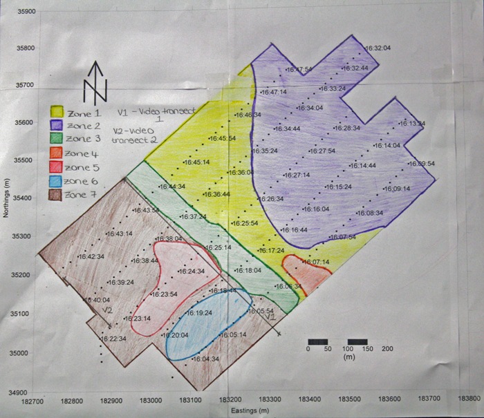
Zone 1

The fairly light shading indicates fine sediment with no obvious bedforms present. A number of wakes can be seen on the trace where turbulence caused small areas of data to be unclear.

Zone 2

Most easterly area and the deepest part of the scan. The trace indicates the sediment here is much finer, seen by the light shading levels. Small seaweed streaks can be seen as small dark dashes.

Zone 3

A clear channel is marked down the centre of the trace, with the use of admiralty charts it can be linked to a channel approaching Mylor harbour. This channel has been dredged to 2.0m however at present it extends approximately 900m from the harbour, most likely due to high boat traffic into the harbour.

Zone 4

The smallest zone on the trace has been outlined due to its darker shading in comparison to zone 1 which encompasses it. There was no video data which could be linked to this zone making it difficult to identify the change. The variation in shading is likely due to a change to coarser sediment or possibly more scallop beds.

Zone 5

The darkest shading occurred at zone 5. Using the video data large areas of scallops and a small amount of Maerl could be identified in this region. Furthermore very small bedforms, due to shallow water influences, could be seen in the northerly section of the zone.

Zone 6

The sidescan data at zone 6 indicated a change in seabed material, and with the use of the video data from the first video transect it can be verified that the change is due to the presence of Maerl beds.

Zone 7

Using both the sidescan and images from the drop camera on the first and second video transects, very dense areas of seaweed were identified across the majority of zone 7.
 

Figure 4.1: Transect lines plotted on computer.

Figure 4.2: Geophysics zoneation map

Geophysics Conclusion

The seabed around the Fal estuary showed variation in sediment properties as a result of the physical conditions of the estuary. The change in substrate across the transects and the range of colours (indicating oxygen levels (black muds are indicative of anoxia)) was prominent;; from fine sediment in zone 1 to coarser sediment in zone 4. The observed range of sediments is a reflection of varying flow speeds and oxygen saturation levels and also explains, to an extent, the subtle change in biota species (more epifauna was seen in areas of larger grained sediments which ensure a greater attachment surface). Coarse sediment was generally found in deeper water channels surrounded by shallower fine sediment areas. Maerl was found in areas of coarser material as fine sediment posed the possibility of smothering and thus killing the maerl (Walters and Hiscock, 2005).

In areas furthest from shore the increased tidal action causes lower diversity and more impoverished conditions. This was observed through the more fragmented maerl and less overall sediment coverage in the video transect towards the centre of the estuary. Conditions closer to the shore promote greater biotic diversity through increased irradiance from shallower water and less influential tidal action, seen in video 2.
Through a combination of ground-truthing video footage and sidescan sonar, a detailed conclusion of the benthic characteristics of the area have been drawn.
 

Conclusions

During the field course, the aim was to utilise the combination of three boat days (Offshore, Estuarine/Pontoon and Geophysical) in order to compare the Fal Estuary and the waters outside of the mouth. Data collection and processing through multi-parameter technique analysis allowed for comparison of the chemical, biological and physical characteristics of the environments.

According to our data thermal stratification throughout the estuary is variable; with distance up the estuary (towards the riverine end) the differences seen between the temperatures of the deep and shallow waters become more pronounced since here the waters are less mixed. This is in comparison to the increased homogeneity seen towards the marine end where tidal mixing is most dominant. Moving out of the estuary, there is less variability in the thermal structure of the water column on both temporal and spatial scales. In this area, there seems to be a more seasonal thermocline compared to the estuarine diurnal thermocline (O’Boyle and Silke, 2010). The thermocline becomes more pronounced with increasing distance offshore since the tidal mixing in deep waters becomes less influential.

Thermal stratification affects density and mixing of the water column. Salinity is also a major controlling factor of density. In general, the Fal estuary is a well-mixed marine water dominated estuary, which has been confirmed by our data set. Homogeneity of salinity is seen significantly far up the estuary with overlying freshwater becoming quickly mixed into the water column due to the strong tidal forcing experience in the area. In contrast to this, the salinity of the offshore waters shows stratification demonstrating increasing salinity with depth. This is due to the longer seasonal thermocline which affects the mixing up of deep water as opposed to the tidal forces acting within the estuary.

The chemical parameters analysed during the field course provide an insight to the processes occurring within the estuary in comparison to offshore. The major nutrients (dissolved phosphate and silicon) show varying depletion in the surface waters offshore; silicon is extremely depleated thus limiting the growth of phytoplankton whereas phosphate remains relatively high throughout the water column. Dissolved silicon decreases in concentration with distance from the estuary. In the estuary there is a high abundance of phosphate, through addition from local agricultural and riverine sources, showing this is not the main limiting factor on phytoplankton growth in the Fal. The dissolved silicon results show a slight removal from the estuary although generally follow the TDL which indicates that they are mainly influenced by end member mixing.

 
The offshore chlorophyll readings show a chlorophyll maximum just below the thermocline, which according to previous studies (Pingree et al, 1977) shows a dinoflagellate bloom, as dinoflagellates are more tolerant to lower light levels and tend to bloom closer to summer. There was no observed change in dominant species between offshore and estuarine waters; both identified to be diatoms. This could be due to the unusually wetter weather experienced over the sampling period causing greater terrestrial run off and increased nutrients. This would favour a prolonged blooming of diatoms. The population dynamics of the zooplankton differ between estuarine and offshore waters; although at both locations copepods are abundant, they are the most abundant in estuarine waters where there is more algal biomass for food. Offshore there is an increase in the proportion of gelatinous zooplankton such as hydromedusae due to their lower metabolic rate.

The flow of the estuarine water column is controlled by the tidal forcing, and reached up to 0.55m/s at the mouth of the estuary and a minimum of <0.01m/s in the middle of the estuary. The flow was greatest over the deep water channel which meanders down the centre of the estuary. The flow rate seems follow the curvature of the channel; with areas of faster flow on the outside of the meander and slower on the inside. This is supported by the backscatter ADCP data which shows an increase in acoustic backscatter in the slower areas inside the meander, indicating higher biomass in the water column. Where flow was high enough maerl beds are supported (confirmed by geophysical sidescan surveying and video ground-truthing of the area). The sidescan survey tracks also showed a variability of grain sizes, from fine mud to broken shell which was confirmed in the video samples.

Overall the successful multi-parameter methods have allowed a multitude of data to be collected. Some scientifically sound conclusions can be drawn about the three dimensional physical, chemical and biological characteristics of the water column, which support previous studies, and the two dimensional topography and geophysical characteristics of the sea bed. If further investigation opportunity should arise it would be valuable to take more samples along the front to explore further the frontal characteristics. In addition samples from further up the estuary (towards the riverine end) would allow the extension of dissolved nutrient data and an increase in the overall accuracy of the estuarine mixing diagrams. However due to general lack of experience in planning an investigation, combined with some lack of time and equipment failure/ unreliability, further research is needed to draw solid conclusions.
 

References

Bien, G., Contois, D. and Thomas, W., 1958, "The Removal of Soluble Silica from Fresh Water Entering the Sea", Geochimica Et Cosmochimica Acta Volume 14.1, Issue 2, Pages 35-54

Cadee G.C. 1978, 'Primary production and chlorophyll in the Zaire River, Estuary and Plume, Netherlands', Journal of Sea Research, 12, 368-381

Cushing D.H. 1989, 'A difference in structure between ecosystems in strongly stratified waters and in those that are only weakly stratified.' Journal of Plankton Research, 11, 1-13.

Garnier, J., Beusen, A., Thieu, V., Billen, G. and Bouwman, L., 2010, ‘N:P:Si nutrient export ratios and ecological consequences in coastal seasevaluated by the ICEP approach’, Global Biogeochem. Cycles, doi:10.1029/2009GB003583, in press.

Gowen R.J., McCullough G., Kleppel G.S., Houchin L. and Elliot P. 1999, 'Are copepods important grazers of the spring phytoplankton bloom in the western Irish Sea?' Journal of Plankton Research, 21, 465-483

GRASSHOFF, K., EHRDARDT, M.,  KREMLING, K. AND ANDERSON, L. G., 1999, ‘Methods of seawater analysis’, Wiley.

Irigoien X., Harris R.P., Head R.N. & Harbour D. 2000. 'North Atlantic Oscillation and spring bloom phytoplankton composition in the English Channel'. Journal of Plankton Research 22, 2637-2371

Lampert W. 1989. 'The adaptive significance of diel vertical migration of zooplankton.' Functional Ecology, 3, 21-27

Longston, W. J., Chesman, B. S., Burt, G. P., Hawkins, S. J., Readman, J. and Worsford, P. 2003, 'Characterisation of the south-west European marine sites: the Fal and Helford cSAC', Marine Biological Association, 8

Menesguen A. & Hoch T. 1997. Modelling the biogeochemical cycles of elements limiting primary production in the English Channel. I: Role of thermohaline stratification. Marine Ecology Progress Series 146: 173-188.

Morris, A., Bale, A. and Howland, R., 1981, "Nutrient Distributions in an Estuary: Evidence of Chemical Precipitation of Dissolved Silicate and Phosphate", Estuarine, Coastal and Shelf Science Volume 12, Issue 2, Pages 205-16

Mortimer, R.J.G. et al. 1999, 'Sediment-Water Exchange of Nutrients in the Intertidal Zone of the Humber Estuary, UK', Marine Pollution Bulletin, 37, 261-279.

Mullin, J. B. and Riley, J. P.,1955, ‘The spectrophotometric determination of silicate-silicon in natural waters with special reference to sea water’, Anal Chim Acta, Volume 12, Pages 162-170

Parsons, T. R., Maita, Y. and Lalli, C. 1984, 'A manual of chemical and biological methods for seawater analysis', pergamon press, new york, 173

Pirrie et al., 1995, ‘Mineralogical and Geochemical Signiture of Mine Waste Contamination, Tresillian River, Fal Estuary, Cornwall, UK’, Environmental Geology,  Volume 29, Ed:1-2, Pages 58-65

Rockwell G.W., Trowbridge J.H. & Bowen M.M. 2000. The Dynamics of a Partially Mixed Estuary. J. Phys. Oceanogr. (30): 2035–2048.

Somerfield, P. J., Gee, J. M. and Warwick, R. M., 1994, "Soft Sediment Meiofaunal Community Structure in Relation to aLong-term Heavy Metal Gradient in the Fal Estuary System", Marine Ecology Progress Series, Volume 105, Pages 79-88

Sommer U. 1994, 'The impact of light intensity and day length on silicate and nitrate competition among marine phytoplankton', Limnology and Oceanography, 39, 1680-1688

Struyf E. et al., 2010, 'The global biogeochemical silicon cycle', Silicon, 1, 207-213

Sverdrup H.U. 1953, 'On conditions for the vernal blooming of phytoplankton', J. Cons. Explor. Mer, 18, 287-295.

Tilman D. and Kilham S.S. 1976, 'Phosphate and Silicate growth and uptake kinetics of the diatoms Asterionella Formosa and Cyclotella meneghiniana in batch and semi-continuous culture', Journal of Phycology, 12, 375-383.

Welch, E. B. and Isaac, G. W. 1967, 'Chlorophyll variation with tide and with plankton productivity in an estuary', 39, 360-366