INTRODUCTION

Welcome to the website of Group 10 for the Falmouth Field-course. The results of our research into the marine and estuarine environment around Falmouth are presented on this page. The field-course took place from 26th June-7th July 2012. (All times in UTC)

COURSE AIMS

The aim is to investigate the unique physical, biological and chemical properties of the Fal estuary through a variety of techniques. The properties of the water column both within the estuary and offshore will be examined along with, how the Fal estuary acts as a transition zone between freshwater inputs and salt water and also, how vertical mixing processes offshore influence the distribution of plankton communities. Furthermore, a geophysical survey of Carrick Roads will be conducted to gain an idea of its benthic communities.

ABSTRACTS

OFFSHORE

BLACK ROCK

At station 1 at Black Rock it was found that the Oxygen saturation profiles decreased from 290% saturated at 2m to 270% saturated at a depth of 10m. Silicon levels also decreased from a concentration of 1.02µmol/l at 2m depth to 0.79µmol/l at 10m Phosphate levels showed a relative increase from 0.0370µmol/l at 2m depth to 0.067µmol/l at 10m. The salinity did not vary greatly with depth however the surface temperature rapidly decreased from 13.40⁰C to 12.93⁰C between 2.5m and 3.80m then slowly decreased to 12.75⁰C at 23.59m. This weak seasonal thermocline may have occurred due to deep waters and relatively low tidal mixing (Mathews, 1911). The recorded fluorescence fluctuated greatly with depth but generally remained within the range of 0.11 and 0.15mg/m^3,, which can be used as an indicator of phytoplankton growth supported by the chlorophyll and nutrient profiles (Hooligan & Harbour, 1977). The turbidity in the water column increased rapidly within the first 0.52m depth and then remained at a constant value around 3.89% transmission until 27m.

STATION 2

The breakdown of stratification over the course of the sampling period is further supported by the general increase in Ri number, which indicated that the water column is unstable and encourages mixing of previously stratified layers. Transmission increased rapidly in the top ~0.5m up to approximately 3.5% for all times at Station 2 and then remained steady with depth whilst fluorescence remained between 0.08 V and 0.130 mg/m³. This variation may have been due to small scale temporal and spatial changes in currents and nutrient availability. The phytoplankton were found to be not confined to the thermocline due to light levels in the shallow water therefore it was favourable for the plankton to exist in the more nutrient rich water of the denser, saline water. The tide was in flood during sampling which was reflected in the stratified system. The salinity gradient was layer of fresh water overlying more dense saline water and the temperature gradient exhibited a sharp drop in temperature in the same location as the halocline. As water entered the harbour, the stratification broke down, seen from 0945 until 1145 when temperature decreased steadily. Throughout the time series there was increased salinity and decreased temperature with depth, due to cold, saline, and denser water (than freshwater) flowing in from offshore.

ESTUARY

The estuary acts as a transition zone to the ocean with observable gradients for a variety of variables. Generally salinity increased from station2 to station 7, whereas temperature decreased.

Throughout the transect there were clear changes in the chemical, biological and physical components of the estuary. It was found at station 1 there was a much greater turbidity (with an Attenuation coefficient of 2.88m^-2) than at station 7 (k=0.50m^-2). The suspended material was most likely removed by the biological activity of zooplankton, whose abundance increased significantly towards the saline end of the estuary as well as chemical processes in the water column. Throughout the transect oxygen saturation was typically greater than 90%, and an oversaturation occurred at station 5 as values exceeded 100%, and were even as high as 104%. Here there is a peak in chlorophyll concentration of 6.08µg/l therefore indicating a bloom of phytoplankton. The chlorophyll concentration was highest at station 7, however there appeared to be no clear trend between chlorophyll concentration and the position along the estuary.

GEOPHYSICS

Generally it was observed, by using a drop camera, that on the east side of the Carrick Roads section of the Fal estuary there was a high abundance of maerl, with very little exposed sediment. In contrast, the west side had no maerl but a higher species diversity, including large amounts of seagrass as well as larger regions of exposed sediment.

THE LOCATION

PHYSICAL PROPERTIES AND FORMATION OF THE ESTUARY

The Fal estuary is located in the south west of England in Cornwall. It is England’s deepest harbour and is the third largest natural harbour in the world with depths of up to 34m (Cycleau.com, 2004). At the entrance to the estuary spring tides have a macrotidal range of up to 5.3m. However, moving closer to the riverine end of the estuary, a mesotidal range of 3.5m emerges (Pirrie et al.). This change in tidal range within the estuary along with tidal currents of up to 2knots results in a well-mixed estuary.

Fal estuary is a drowned river valley or ria. It was formed through the combination of eustatic sea level rise and isostatic recovery of tectonic plates. The melting of glaciers covering Scotland caused tectonic uplift and led to a sink in land towards the south of England, sea levels have also risen around 125m in the last 180,000 years. The catchment area for the estuary covers 346km2 (Cycleau, 2004) and multiple rivers.

Many important habitats exist throughout the estuary,  for example, muddy, sandy and rocky sublittoral (1736ha), intertidal mudflats (653ha) and salt marshes (93ha). It is also home to many species of scientific interest, for example the calcareous algae, Maerl.  For these reasons, along with the high levels of pollutants, the European Environment Council has designated Fal estuary as a ‘Special Area of Conservation’ and a ‘Site of Special Scientific Interest’.

ANTHROPOGENIC FACTORS

The Fal estuary has become one of the most polluted in England. Tourism, watersports and boat traffic all influence this. However, the estuary’s mining history far exceeds all other impacts on the concentration of pollutants. The surrounding land is rich in ores, particularly those of tin and copper which have been mined through streaming since the Bronze age and in deep mines in the area since as early as the 18th Century (Bryan, G.W. and Gibbs, P.E, 1983). Due to the semi-enclosed nature of the estuary, pollutants become trapped and concentrated to extents that are seen in open water. These heavily influence the biology and chemistry of the water, for example the Wheal Jane incident of 1992 created toxic copper levels in Restronguet creek and led to a more resistant species of N. diversicolor compared to elsewhere in the estuary. Furthermore, high concentrations of TBT (tributyltin) in Carrick roads have been shown to cause imposex in Dog whelks (Nucella lapillus).

GENERAL METHODS

FIELD METHODS

Using an ADCP, information on the velocities, backscatter and depth of the water column was obtained. The ADCP ran continuously throughout each sampling period.

Physical parameters of the entire water column were obtained using a CTD and fluorometer mounted in a rosette sampler. Data for the following physical parameters was collected continuously with depth; temperature, salinity, fluorescence, light transmission, irradiance.

Water samples were taken using Niskin bottles set in the rosette sampler. The depths at which Niskin bottles were fired were determined by looking at the downwards CTD profile and selecting any points of interest based on the physical structure of the water column. This was often at depths of fluorescence peaks, within layers of fresher surface water, or above, below and at the thermocline. These water samples were obtained in order to quantify (following on-shore lab analysis); dissolved silicon, dissolved oxygen, chlorophyll, nitrate and phosphate, phytoplankton abundance and species distribution.

A zooplankton trawl (with 48.5cm diameter, a 200µm mesh net with a 1L sampling bottle) was also used. It was deployed from variable depths depending on distinctive signals of fluorescence and backscatter in the water column.

WET LAB METHODS

Samples were prepared in the wet lab ready for on-shore lab analysis.

Phytoplankton - 50ml of each sample was taken straight from the Niskin bottle and was added to 1ml Lugols Iodine solution to preserve phytoplankton. 

Oxygen - 100ml of each water sample was decanted straight from the Niskin bottle into a glass vial. It was made sure that the water overflowed to remove any bubbles. 1ml of manganese chloride and then 1ml of alkali-iodide were added (Winkler, 1888) and the vial was inverted carefully to mix the solution. Samples were stored in a temperature controlled container.  

Nitrate, Phosphate and Dissolved Oxygen - samples were filtered using GFF filters (0.7 µm) and filtering apparatus. 50ml of each sample were stored in glass (nitrate and phosphate) and plastic (dissolved silicon) containers, which were kept in a temperature controlled environment.

Chlorophyll - the filter papers used to filter the nitrate,  phosphate and dissolved silicon samples were placed in 6ml of 90% acetone and stored in the fridge.

ON SHORE LAB METHODS

CHEMICAL METHODS

Dissolved Silicon– the dissolved silicon analysis was done using a slightly modified method from Mullin & Riley (1955). Using a 5ml hand pipette, 5ml of sample was added to each tube – which then had 2ml molybdate solution added and left for 10 minutes. 3ml of mixed reducing agent was added to all samples, standards and blanks, and then allowed to stand for 2 hours. The mixed reducing agent (MMR) consisted of 10ml metol sulphite, 6ml oxalic acid, 6ml sulphuric acid and 8ml MQ water. Once 2 hours had passed the absorbance of dissolved silicon was measured using a U-1800 Spectrometer set at wavelength of 810nm – the samples were individually added to a 4cm cell which was cleaned before measurements. Construction of a calibration curve from the results obtained can be used to determine the dissolved silicon concentration of each unknown sample.

Phosphate– the methods of Parsons T. R. Maita Y . and Lalli C. (1984) were followed to determine phosphate concentrations.

Dissolved Oxygen – the dissolved oxygen concentration was determined using the method of Grasshoff, K., K. Kremling, and M. Ehrhardt (1999).

Nitrate – concentration was determined using the ‘nitrate by flow injection analysis’ method of Johnson K. and Petty R.L. (1983)

BIOLOGICAL METHODS

Zooplankton - Upon collection using the plankton net, organisms were preserved in diluted formalin. On-shore, zooplankton abundance and species information was obtained by analysing 10ml subsamples in a Bogorov tray under a light microscope.

Phytoplankton- The number of phytoplankton cells per m3 was found by placing 1ml of concentrated sample into a Sedgewick-Rafter chamber. Species were identified, counted using a light microscope and then the resulting number was adjusted for concentration and quantity to find the abundance per m3.

Chlorophyll -  the chlorophyll concentration of each sample was found as stated by Parsons T. R. Maita Y . and Lalli C. (1984).

OFFSHORE BOAT PRACTICAL- Bio - Chemical - Physical - Summary - Back to top

INTRODUCTION

How do vertical mixing processes in the waters off Falmouth affect, directly and indirectly, the structure and functional properties of plankton communities?

The usual trend expected of offshore waters is; a decline in temperature and an increase in salinity with depth, and, a peak in plankton abundance at the thermocline. We predict depletion in nutrients and a decline in the oxygen content of the water where plankton is abundant.  By obtaining chemical, physical and biological data we aim to explain the distribution of plankton communities and compare this to expected trends

OFFSHORE METHOD

FIELD METHODS

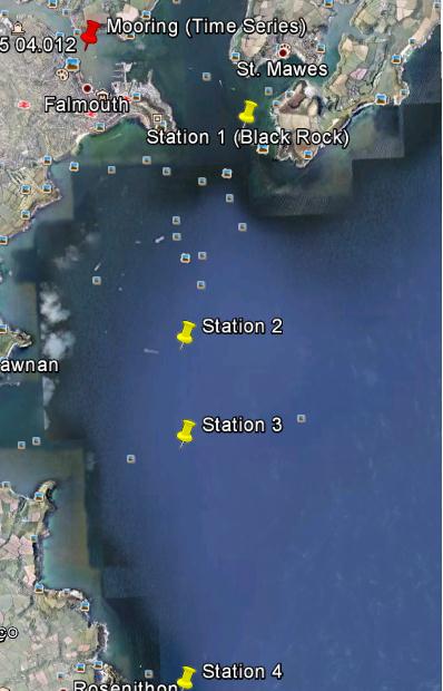
The initial plan for the morning of 27th June 2012 was to follow a transect starting at Black Rock (50⁰08.68N 005⁰01.74W) bearing due south towards Manacles Point (see Figure 2.1). CTD profiles and water samples were to be obtained at 4 sampling stations; Black Rock, Manacles Point, and at two stations between these locations. Upon sampling at Black Rock, heavy fog conditions were observed, deeming the remainder of the planned transect unsafe to execute. Samples were collected at this station along with CTD, fluorometer and ADCP data however; the plankton net was not deployed. Consequently, a revised plan to carry out time-series measurements at a single location in the harbour was adopted. The location of the time-series station (Station 2) deviated about 50⁰09.543N 005⁰04.012W due to the drifting of the vessel (see Figure 2.1). CTD and fluorometer data was collected every half hour starting at 0845 and, every hour water samples were taken at depths of interest. The plankton net was also deployed every hour. See “Field Methods” for more detail.

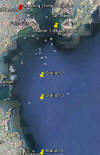
Figure 2.1

Date: 27/06/2012 (day before neap tide)

Table 2.1:

LAB METHODS

Samples were prepared in the wet lab ready for on-shore lab analysis as stated in the “Wet Lab Methods”

Physical - CTD data was managed and graphed using ‘Sigmaplot’. ADCP data was displayed using Winriver.

Chemical - Samples collected were analysed to quantify dissolved silicon, dissolved oxygen, chlorophyll and, nitrate and phosphate. Methods of analysis are stated in “Lab Methods”.

Biological - Both zooplankton and phytoplankton species were identified and counted. The exact method is stated in “Lab Methods”.

BLACK ROCK (STATION 1)

RESULTS

PHYSICAL

ADCP

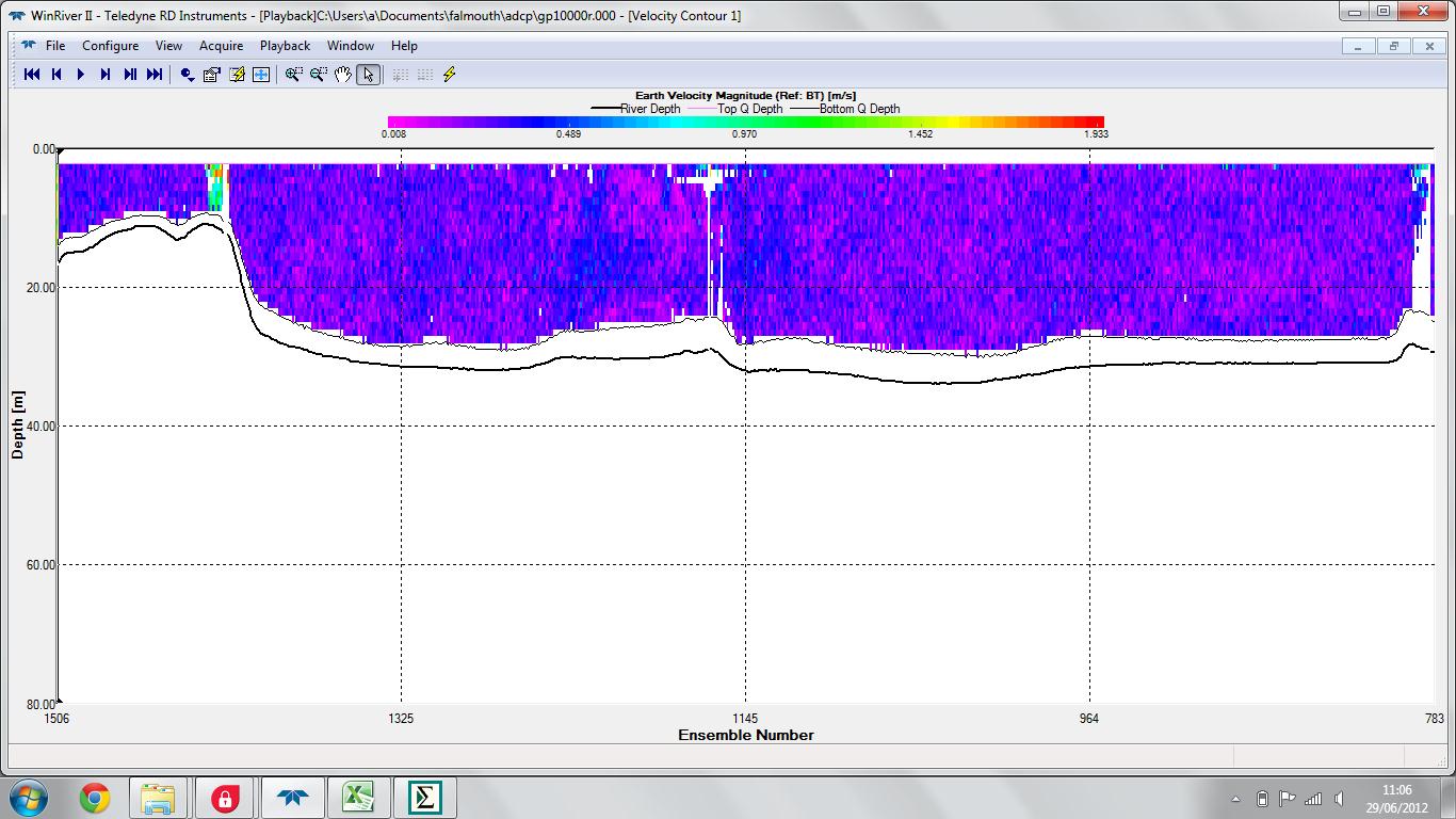
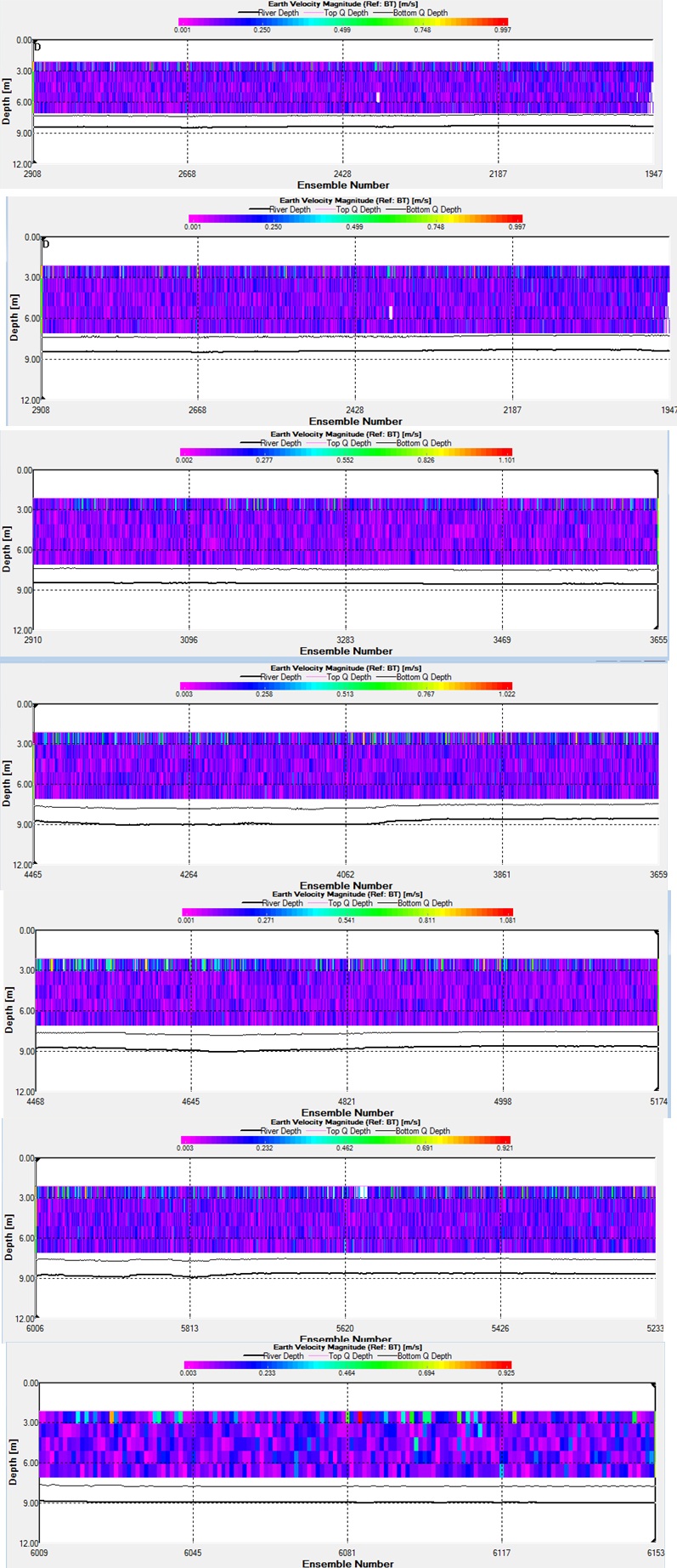
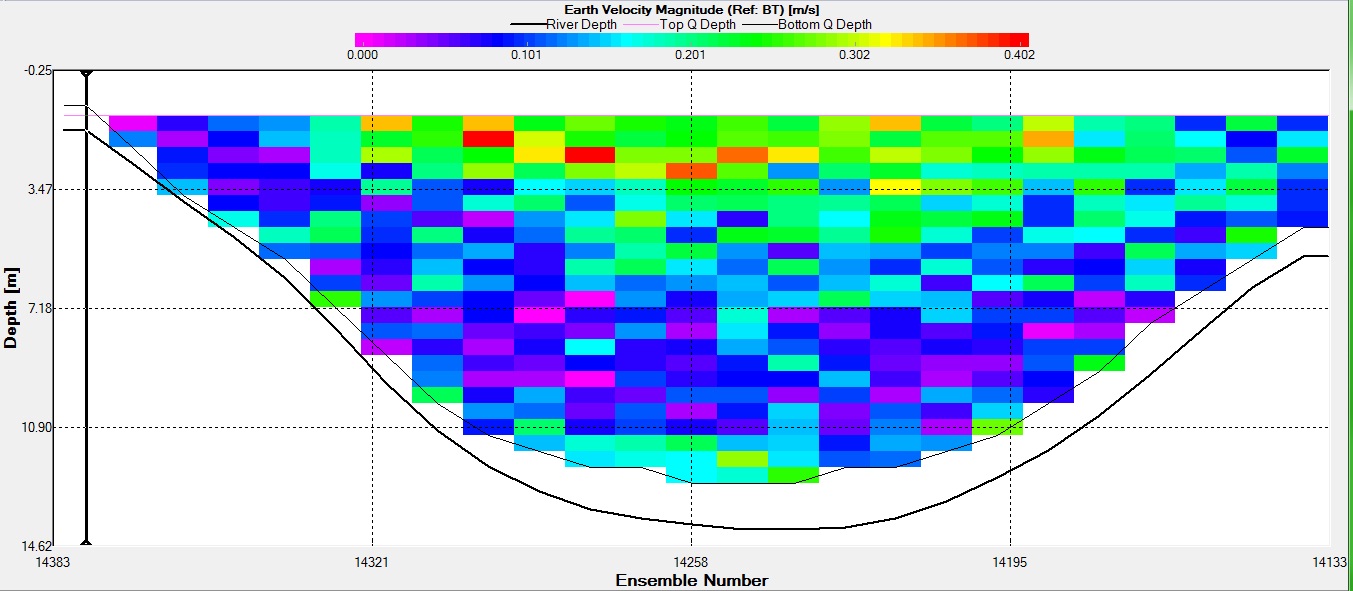
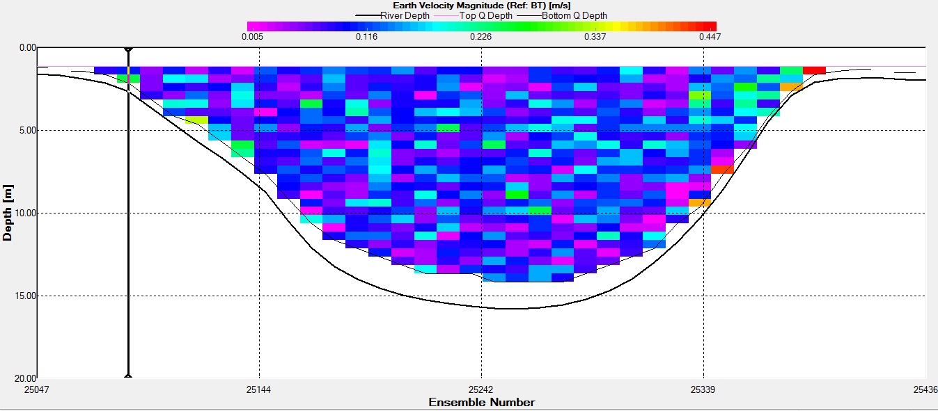
Velocity appears to vary little with depth at station 1 (fig. 3.3), there is an area of greater velocity in the far west of the plot, this rapid increase in velocity with maximum velocity of  ~ 1ms-1, this patch of rapidly increased velocity may be an anomaly as it is significantly greater  than the water surrounding it. Although it may also be related to the rapid change in topography of the sea bed at the same location.

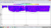
Figure 3.3: ADCP profile showing flow rate (m/s) from Station 1 (Black Rock) at 0745 UTC

CTD

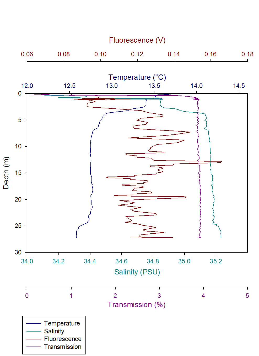
Figure 3.2 Illustrates the CTD data obtained at the first station, Black Rock. The surface temperature recorded was 13.40⁰C which remained constant until around 2.02m depth before rapidly decreasing between depth 2.5m and 3.80m to a temperature of 12.93⁰C. The temperature then decreases slowly, and remains constant at 12.75⁰C until a depth of 23.59m. Temperature decreased to 12.58⁰C by the end of the profile at 26.92m depth. The fluorescence data on the CTD fluctuated greatly with depth but generally remained within the range of 0.11 and 0.15V with a few exceptions such as at the surface of 0.10V and peaks of increased fluorescence at 12.82m a value of 0.17V. Transmission was used as an indication of turbidity in the water column and was lowest at the surface, and increased rapidly within the first 0.52m depth of the water column and then remained at a constant value around 3.89% until 27m. The salinity did vary significantly with depth, at 0.28m the lowest recorded salinity was 34.10 which increased to 35.1 at 3.85m. After this, salinity remained constant as depth increased, with an exception of a slight increase to 35.23 at 25.95m depth.

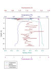
Figure 3.2: CTD data measuring temperature (⁰C), fluorescence (V), salinity and transmission (%) measured at Station 1 (Black Rock) at 0745 UTC

LIGHT

Table 3.1 Station 1 light attenuation information. The equation of the regression line and negative reciprocal of the gradient of the line. From this gradient K_sensor is calculated. Secchi depth is recorded in meters. This sechi depth is used to calculate a second light attenuation coefficient (K_Secchi).  The final column shows the range between these two light coefficient values.

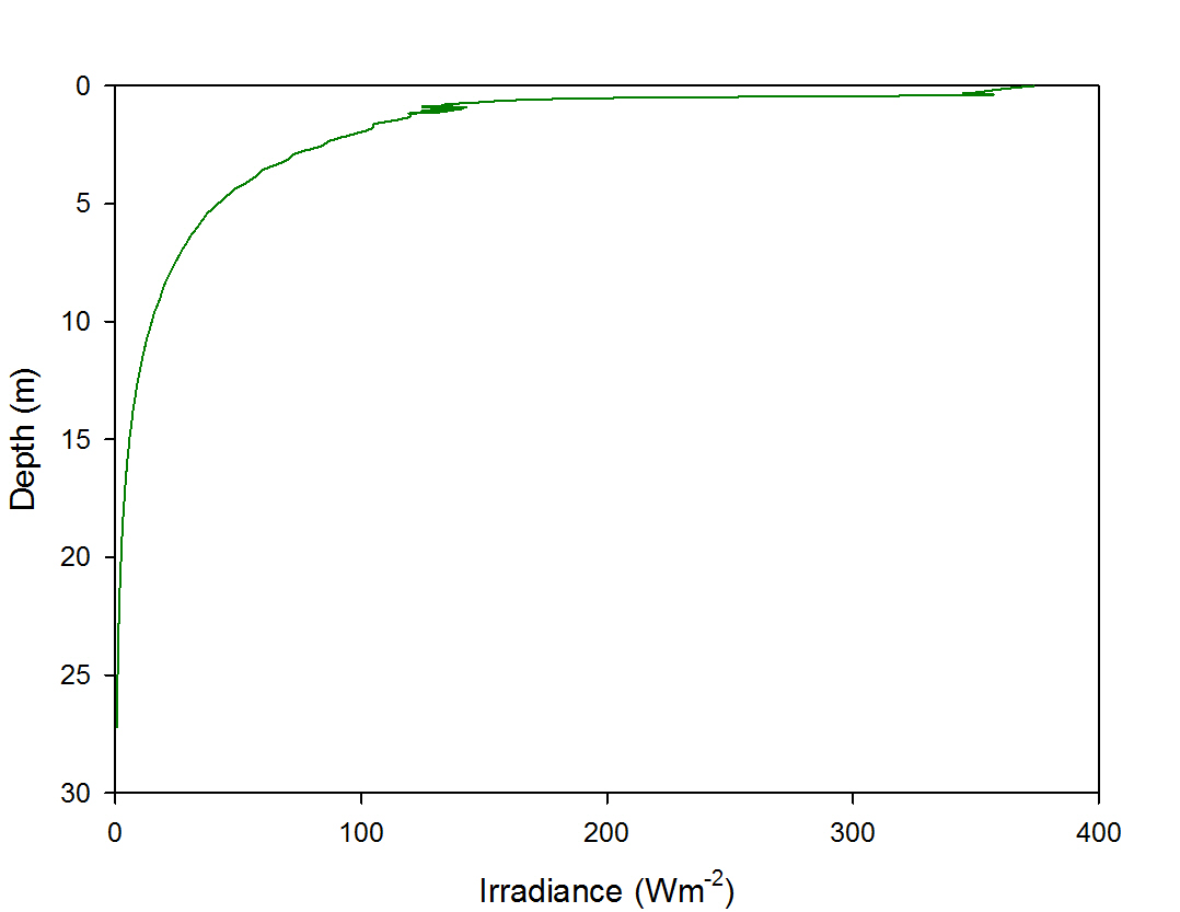
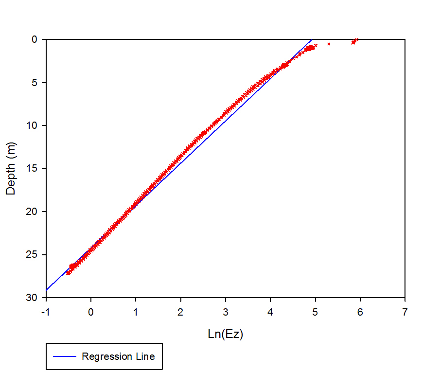
Station 1 has a surface light irradiance of ~375m^-2, (Figure 3.5) as depth increases light irradiance decreases exponentially, a significant decrease in irradiance is shown over the surface 5m, with light irradiance values of ~40Wm-2 at 5m depth.  1% of surface light irradiance is found at ~17.5m depth.  The natural log of light irradiance against depth (Figure 3.6) follows a relatively straight line between depths of ~3m and the maximum depth of the profile, the top 3m of the water column show a greater Ln(Ez) value than expected.  The equation of the regression line shown in figure P, is shown in table T.  Using the negative reciprocal of the gradient of the regression line the attenuation coefficient can be calculated (K_sensor ). The attenuation coefficient calculated from the Secchi depth (K_secchi) is also shown in table T.  These two different attenuation coefficients appear to show a significant difference, with K_secchi being ~40% greater than K_sensor

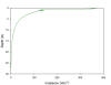
Figure 3.5: light irradiance curve from CTD data measured in Wm^-2 at Station 1 (Black Rock) at 07.45 UTC

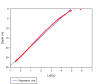
Figure 3.6: natural log of light irradiance(ln(Ez)) with depth from CTD data at Station 1 (Black Rock) at 07.45 UTC

Table T Station 1 light attenuation information. The equation of the regression line and negative reciprocal of the gradient of the line. From this gradient Ksensor is calculated. Secchi depth is recorded in meters. This sechi depth is used to calculate a second light attenuation coefficient (KSecchi).  The final column shows the range between these two light coefficient values.

CHEMICAL

The Station 1 chemical data was recorded from two depths. The Oxygen saturation profile decreased from 107% saturated at 2m to 99% saturated at a depth of 10m .Dissolved silicon levels also decreased with depth, a concentration of 1.02 µmol/l at a depth of 2m was recorded. This then decreased to 0.79 µmol/l at 10m. Phosphate levels showed an increase from 0.037 µmol/l of phosphate recorded at 2m to 0.067 µmol/l at 10m.

BIOLOGICAL

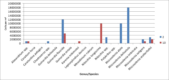
Figure 3.4: Shows a larger abundance of phytoplankton at 2m than 10m. Guinardia flaccida, Rhizosolenia alata and Rhizosolenia delicatula are the most abundant species present in the water column at this time. With cell count estimates of 1.2 x 107, 1.8 x 107 and 1 x 107 per m3 respectively. Species diversity is low at this time.

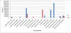
Figure 3.4: phytoplankton cell count from water samples taken at 2 and 10m depth measured in cells per m³ at Station 1 (Black Rock) at 0745 UTC

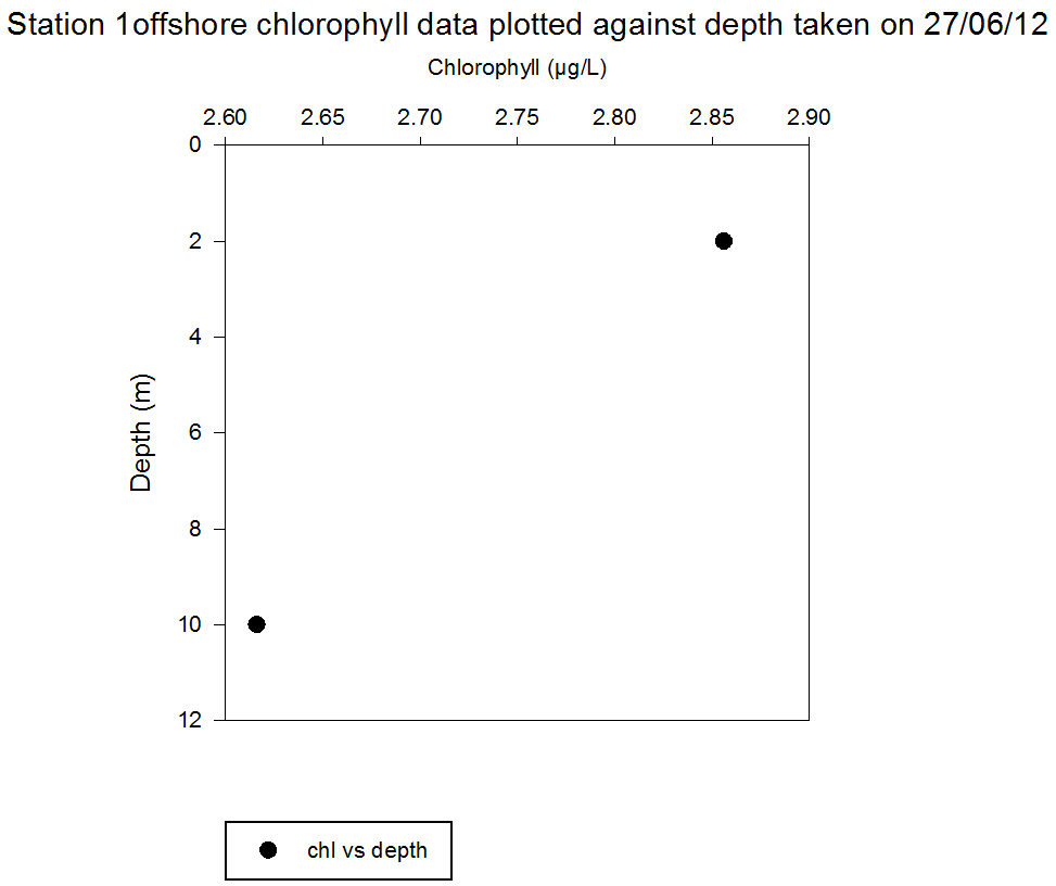
Figure 3.7 illustrates that the highest chlorophyll measurements taken at both a shallow depth of 2m and the deepest depth of 10m were taken at the first station at Black Rock.

Figure 3.7 Chlorophyll (µg/l) measured in the lab by Fluorometer from Niskin bottle samples at Station 1 (Black Rock) at 07.45 UTC

DISCUSSION

The weak thermocline and strong halocline indicates a shallow cold less saline surface layer of the water column. These physical gradients occur within the first 5m. In the Western English channel a weak seasonal thermocline occurs due to deep waters and relatively low tidal mixing (Mathews, 1911) This is supported by the Richardson number data, which shows laminar flows in the surface 10m.  The halocline is formed by output of less saline so therefore less dense water from the River Fal. This is more buoyant than the cooler, more saline waters of the Western English Channel and creates a strong salinity gradient.

The 2m sample collected water from above the apparent thermo and haloclines, the 10m sample retrieved from below.  The shallow water sample indicated low phosphate, high dissolved silicon levels. The CTD fluorescence data (Figure 3.7) depicts the surface waters to be relatively low in chlorophyll compared to data collected at depth. However phytoplankton cell counts taken at 2m and 10m illustrates phytoplankton abundance to be greater in the surface water than further down the water column.  The chlorophyll concentration calculated from the water samples, support the fluorescence data collected by the CTD, as it shows a greater concentration at 10m than 2m. This supports the theory that phytoplankton growth becomes limited by the depletion of nutrients (Hooligan & Harbour, 1977).

Figure 3.7 illustrates that the highest chlorophyll measurements taken at both a shallow depth of 2m and the deepest depth of 10m were taken at the first station at Black Rock.

TIME SERIES (STATION 2)

PHYSICAL RESULTS

ADCP

The ADCP data at Station 2 (Figure 4.1) shows velocities ranged between 0.001 m/s and 0.250 m/s throughout the times series. The layer of water between 2.59m and 3.00m exhibits faster flow velocities of up to around 0.400m/s throughout the time series.

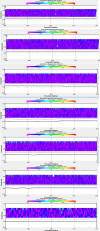
Figure 4.1: ADCP flow rate profiles (m/s) taken between 0815 and 1115 every half hour at Station 2

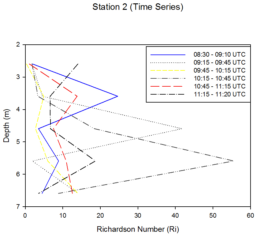
RICHARDSON NUMBER

The Richardson number is a dimensionless number used to evaluate the mixing conditions in the water column.

The Richardson number was calculated using averages over the course of every half hour at Station 2 and once at Station 1.

At 0845 the Richardson number remained under 0.2500 for most of the water column with the only exceptions at 2.59m (Ri=0.2787) and 6.59m (Ri=0.4348). This was also true for the water column at 0915 with the only exception being 0.3032 at 2.59m. At 0945, Ri increased with depth beginning at 0.0404 at 2.59m and increasing to 0.7860 at 6.59m, however, Ri did not surpass 1.0000. At 1015, the Richardson number remained above 0.2500 for the entire water column apart from at 2.59m and 4.59m where Ri was 0.1359 and 0.1057 respectively. The Richardson number at 1045 was lowest at 3.59m at a value of 0.0461 and the maximum Ri was 13.9767 at 6.59m. At 1045, Ri increased with depth. At 1115, Ri was over 1.0000 at depths of 3.59m and shallower however, this rose rapidly to 3881.3185 at 4.59m and then proceeded to drop again to 0.6661 at 5.59m and then again to 0.0592 at 6.59m (Figure 4.2).

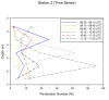
Figure 4.2: Time series of Richardson numbers (Ri) taken between 0830 and 1120 calculated using ADCP data at Station 2

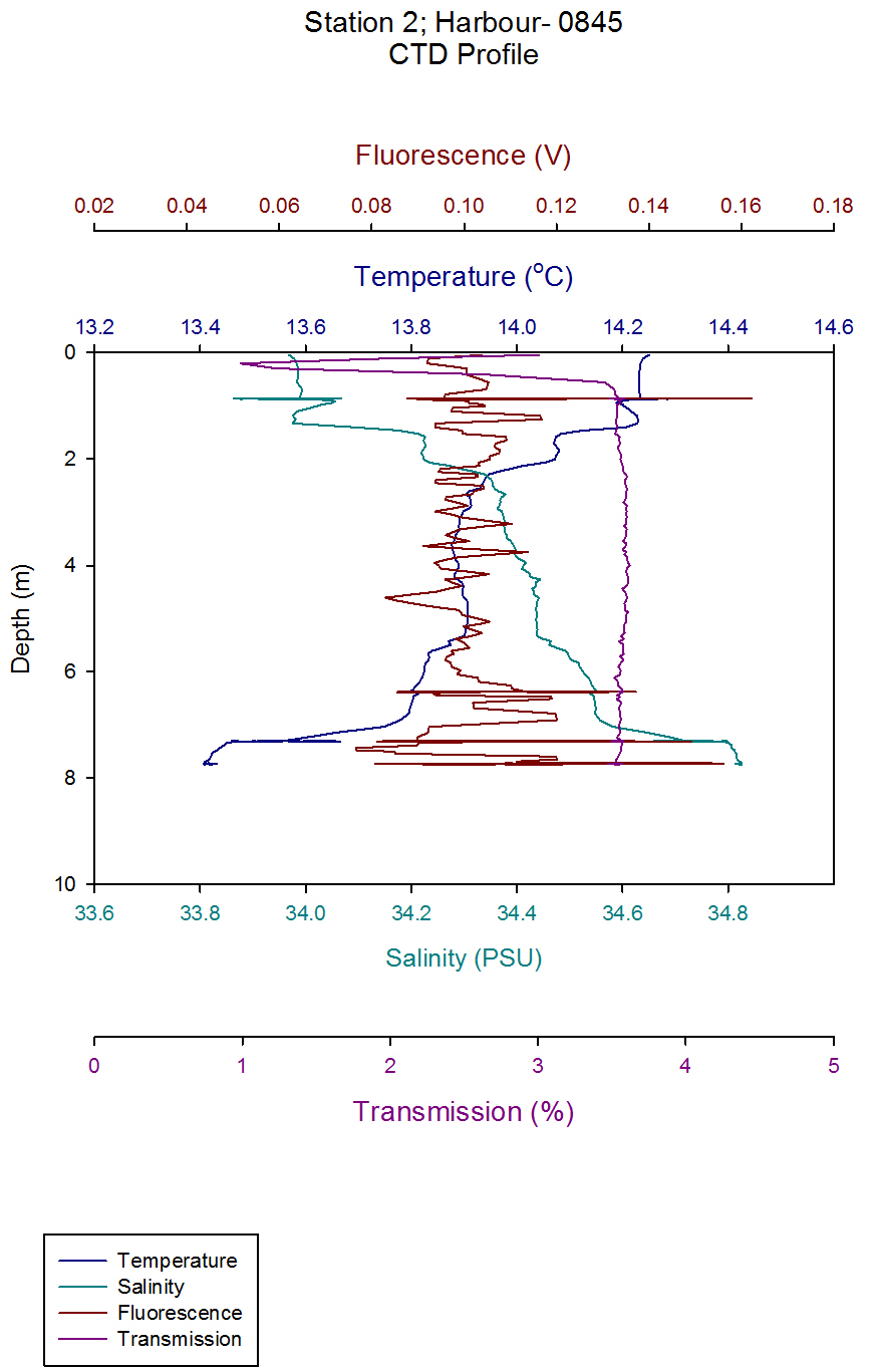
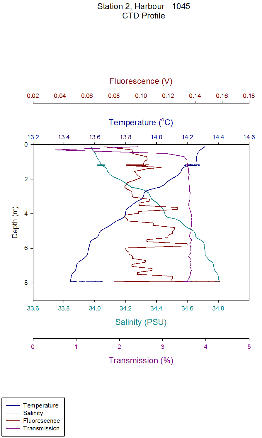
CTD

Note:  in order to gain accurate results with the CTD profiler, it was necessary to lower the sampler to just below the surface (commonly around 1.00m depth) for a few minutes, allowing it adjust to the condition of the water column. It is for this reason that there may be horizontal 'lines' of data in places, where the CTD was adjusting. Transmission values are also high upon entering the water which is a result of the instrument adjusting to the transition from the air to the water.

A 1.25m thick fresher surface water layer was evident in Figure 4.3, with a salinity of 34.00. Below this depth was a halocline, extending to 2.45m depth with salinity increasing to 34.35. Below the halocline, salinity increased gradually to 34.55 by 6.79m depth. Another sharp increase in salinity was noted at the bottom of the profile, increasing to 34.82 by 7.59m depth. The temperature data also indicated a different surface layer 1.25m thick with a temperature of 14.2⁰C. Below this layer a thermocline was evident, extending to a depth of 2.60m and decreasing to 13.91⁰C. The temperature stayed fairly stable for the remaining depths; however, it decreased rapidly from 13.79⁰C to 13.42⁰C between depths of 6.79m and 7.64m. Transmission increased to 3.45 by 0.55m depth, and remained between 3.50%-3.60% as depth increased. Fluorescence fluctuated greatly throughout the water column but remained within a range of 0.09V and 0.11V, with the exception of the large peaks at the depths 0.87 m, 7.31m and 7.68 m, which reached values of 0.16V.

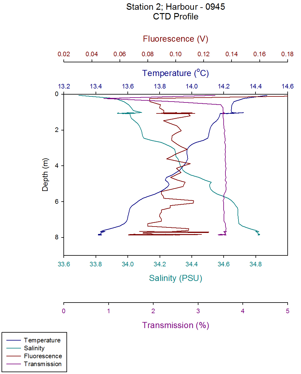
Figure 4.4 shows the physical parameters of Station 2 at 0915. A surface layer of water 1.75m thick had a temperature of around 14.15⁰C. By 2.2m depth temperature had rapidly decreased to 13.95⁰C, representing a thermocline. Below this depth, temperature remained fairly constant, until a sharp decrease from 13.83 to 13.55⁰C between 6.38m and 7.36m depth. The surface layer was also characterised by a lower salinity than the rest of the water column, of around 34.00 in the top 1.75m. Below this depth, salinity gradually increased to 34.73 at 7.36m depth. Fluorescence fluctuated from 0.07V to 0.12V throughout the water column. Transmission increased to 3.58% by a depth of 0.60m, and beyond this depth remained constant

.

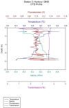
 Figure 4.4: CTD data measuring temperature (⁰C), fluorescence (V), salinity and transmission (%) measured at Station 2 at 0915

Data acquired at 0945 displayed in Figure 4.5 appeared to show no distinctive surface layer as seen in previous time-series profiles. Salinity increased fairly steadily from 33.69 to 34.81 over the 7.78m profile. Temperature also decreased steadily over this depth, from 14.47⁰C to 13.43⁰C. After an initial increase in the top 0.50m of the water column, transmission remained close to 3.61% throughout the whole profile. Fluorescence fluctuated between the values 0.08V and 0.12V with the lowest value at the surface of 0.08V and a peak at 7.88m depth with a value of 0.13V.

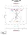
Figure 4.5: CTD data measuring temperature (⁰C), fluorescence (V), salinity and transmission (%) measured at Station 2 at 0945

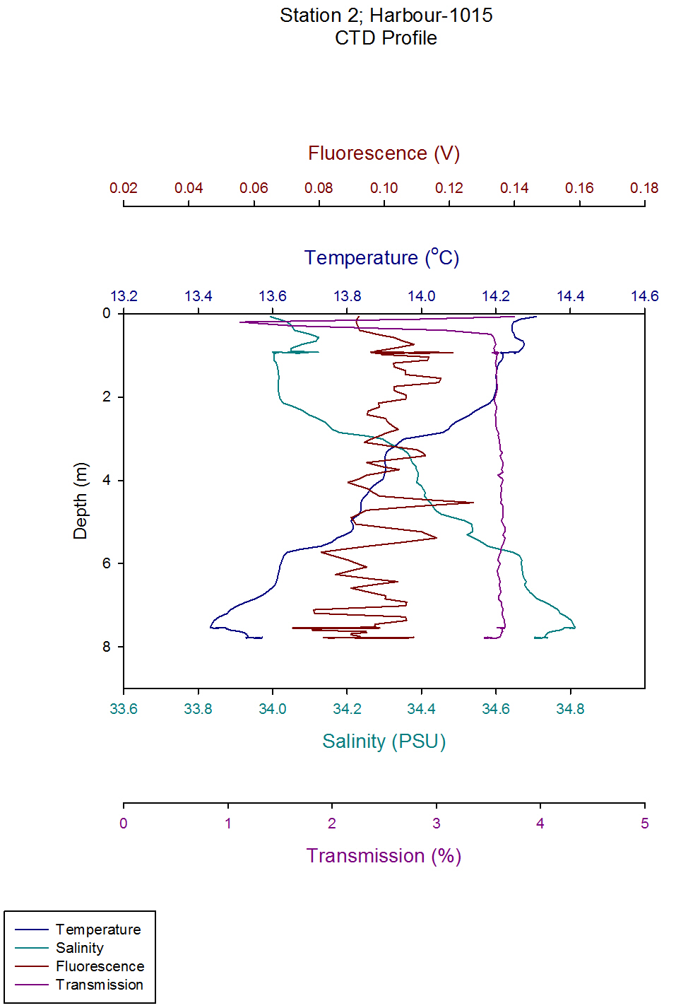
The time-series profile of Figure 4.6 (recorded at 1015) appeared to show a distinct surface layer, despite this stratification not being present in the profile acquired 30 minutes prior (Figure 5.5).  Salinity data suggested a surface layer thickness of 2.04 m, with a salinity of 34.02. Below this depth, salinity increased to 34.81m at 7.45m. Interestingly, below this depth until 7.78m salinity decreased to 34.72. Temperature showed an inverted distribution to salinity, with a 1.98m thick surface layer of 14.19⁰C. Below this depth, until 7.45m, temperature decreased gradually to 13.44⁰C, before increasing to 13.56⁰C by 7.78m. Again, fluorescence greatly fluctuated with depth, remaining within the range of 0.09V and 0.11V. The greatest peak occurred at a depth of 4.53m with a value of 0.13V. Transmission increased to a value of 3.52% by 0.49m depth, then remained fairly constant throughout the profile with the exception of a slight decrease at 7.78m.

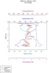
Figure 4.6: CTD data measuring temperature (⁰C), fluorescence (V), salinity and transmission (%) measured at Station 2 at 1015

In Figure 4.7 temperature decreased steadily from 14.30⁰C to 13.44⁰C over the entire 7.88m of the profile. Salinity increased steadily with depth throughout the profile from 33.98 to 34.81. Transmission increased to 3.50% in the top 0.69m, and remained close to 3.60-3.70% for the remainder of the profile. Fluorescence fluctuated within the range of 0.09V and 0.13V with the smallest fluorescence value of 0.07V recorded at the surface and the greatest at 7.95m depth of 0.16V.

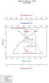
Figure 4.7: CTD data measuring temperature (⁰C), fluorescence (V), salinity and transmission (%) measured at Station 2 at 1045

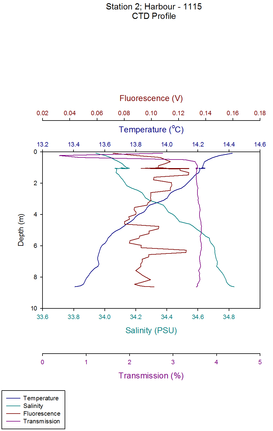
Figure 4.8, showing a profile taken at 1115, illustrates that temperature decreased from 14.43⁰C at the surface to 13.42⁰C at 8.62m depth. Salinity increased from 33.95 to 34.83 from the surface to 8.62m depth.  Transmission increased to 3.56% rapidly within the top 0.88 m, and remained constantly near this value for the remainder of the profile. Fluorescence values fluctuated from 0.07V to 0.13V throughout the whole profile.

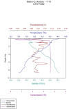
Figure 4.8: CTD data measuring temperature (⁰C), fluorescence (V), salinity and transmission (%) measured at Station 2 at 1115

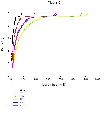
The greatest surface irradiance was found at times 0945 and 1015 (Figure 4.9).  It is also appears that very little light was absorbed in the surface ~30cm of the depth profiles,  as here the gradient of the light irradiance curve is near vertical. This could be due to the sensor being located at the highest point on the rosette sampler,  and the depth reading being taken from the bottom of the sampler.  At most depths the natural log of Ez followed a near straight line (Figure 4.10).  In surface waters the linear relationship was altered, which could again be due to the location of the CTD on the rosette sampler.

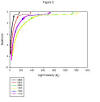
Figure 4.9: time series of light intensity (Ez) measured using a fluorometer at Station 2 between 0845 and 1115

The attenuation coefficients calculated from the light sensor on the CTD (Ksensor) showed a greatest value of 0.461m^-1 at 1015, and a lowest value of 0.334m^-1 at 0845. The range between these is equal to 0.127m^-1, which is over 25% of the value at 1015. This showed a significant change between stations, however there appeared to be little relationship with time.   The three attenuation coefficients calculated with the Secchi disk depths showed a maximum value of 0.36m^-1 at 0845, and a minimum value of 0.29m^-1 at 1045. The range here was also significant as it was equal to ~20% of the KSecchi value at 0845. There appeared to be an inverse relationship, as the attenuation coefficient decreased as time increased.

Table 4.1: Includes the equation of each regression line shown in Figure 4.10, the gradient of these lines multiplied by -1, The equation used to calculate Ksensor, as well as the Ksensor value. Also shown is the Secchi disk depth for those times where a Secchi depth had been recorded.  This is then used to calculate another attenuation coefficient KSecchi, this is done by dividing 1.44 by the secchi depth (m). The final column shows the range between the two attenuation coefficients calculated

Figure 4.1: ADCP flow rate profiles (m/s) taken between 0815 and 1115 every half hour at Station 2 

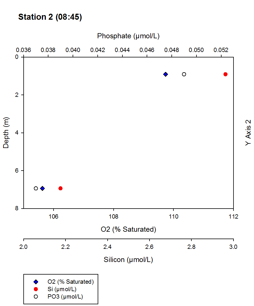
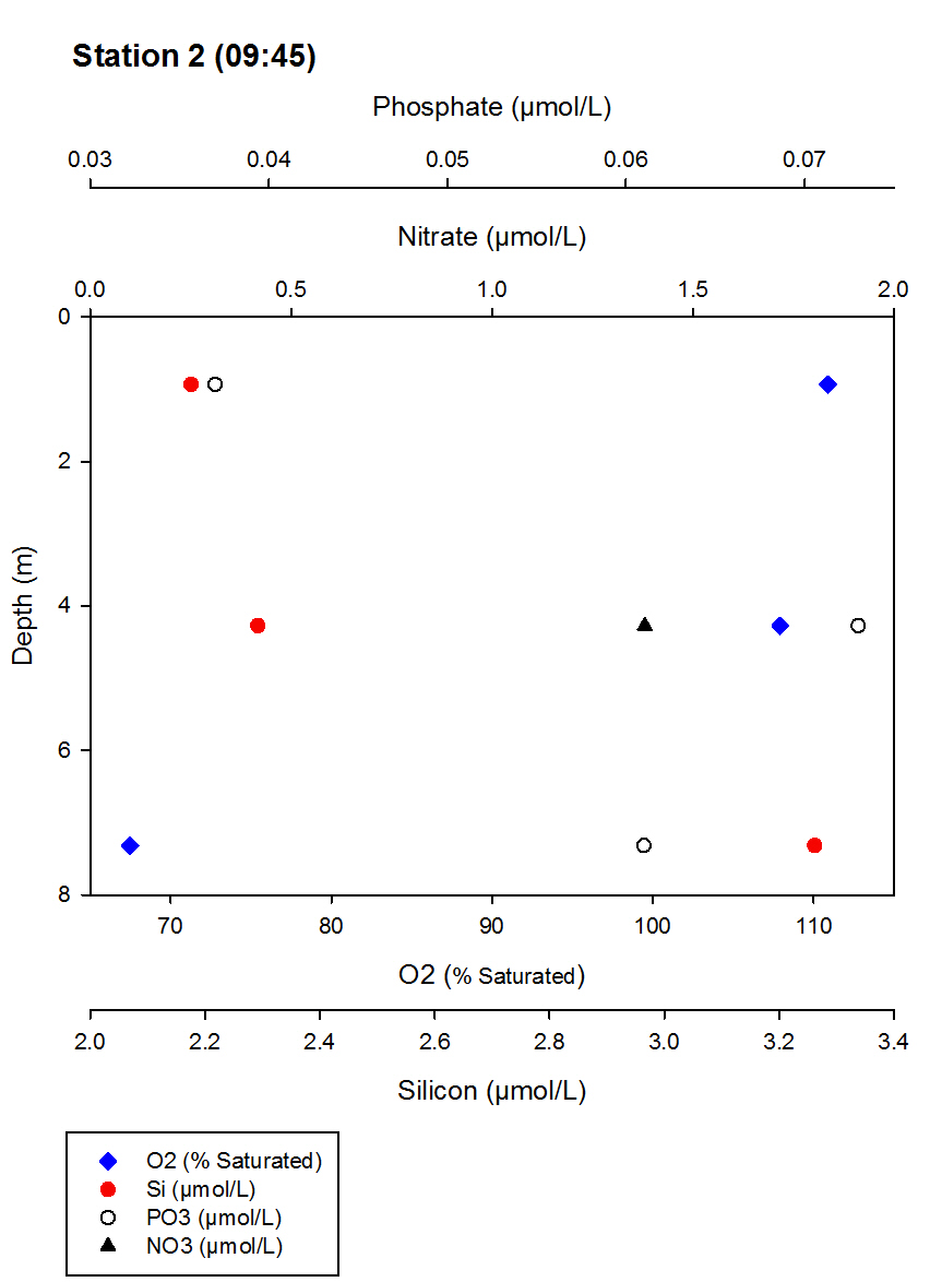
CHEMICAL RESULTS

At 0845 dissolved oxygen decreased from 109% saturation at a depth of 0.91m to 105% saturation at 6.94m. Dissolved silicon levels also declined from 2.96 µmol/l at 0.91 to 2.18µmol/l at 6.94m. Phosphate levels decreased from 0.049 µmol/l to 0.037µmol/l over the same depth range (Figure 5.1).

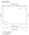
Figure 5.1: Phospohate (µmol/L), Silicon (µmol/L) and 02 (% saturation) profiles at Station 2 at 0845

At 0945, dissolved oxygen dropped from 110% saturation to 67% over 7.32m, with the steepest drop from 107% at 4.27m to 67% at 7.32m. Dissolved silicon levels increased from 2.18µmol/l at 0.93m to 2.29 µmol/l at 4.27m and then 3.26 µmol/l at 7.32m. Phosphate concentrations increased from 0.037 µmol/l at 0.93m to 0.073µmol/l at 4.27m, and then decreased slightly to 0.061 µmol/l at a depth of 7.32m (Figure 5.2).

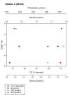
Figure 5.2: Phospohate (µmol/L), Silicon (µmol/L) and 02 (% saturation) profiles at Station 2 at 0845

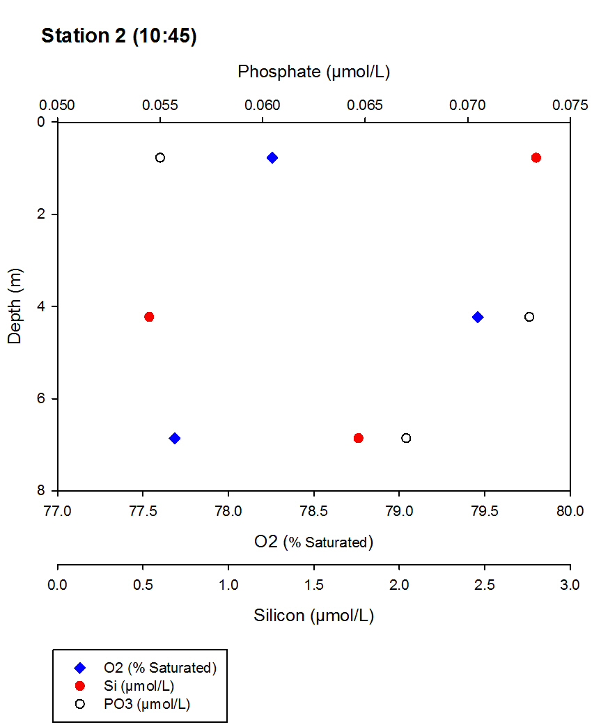
At 1045, the oxygen concentration rises from 78% at 0.77m depth to 79% at 4.23m. It then declined slightly to 77% at 6.86m. Dissolved silicon levels decreased from 2.80µmol/l at 0.77m to 0.54µmol/l at 4.23m, then increased slightly to 1.76µmol/l at 6.86m. Phosphate levels at 1045 Station 2 followed a similar pattern to oxygen concentration with a slight increase of 0.055µmol/l at 0.77m to 0.073µmol/l at 4.23m, then decreasing to 0.067µmol/l at 6.86m (Figure 5.3).

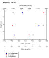
Figure 5.3: Phospohate (µmol/L), Silicon (µmol/L) and 02 (% saturation) profiles at Station 2 at 10.45

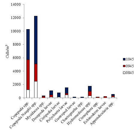
BIOLOGICAL RESULTS

Figure 6.1 shows there are 2 groups which were dominant throughout the time series, Copepoda and Copepoda Nauplii, with Copepoda numbers varying from 1191 cells/m³ to 4546 cells/m³ whilst Copepoda Nauplii numbers varied from 2490 cells/m³ to 7144 cells/m³. It can be seen that the majority of groups increased in number from 0845 to 1045; and groups that increased over the time series included Copepoda, Copepoda Nauplii, Decapoda Larvae, Cirripedia Larvae, Hydromedusae and Appendicularia. Groups that were not present at the start of the time series but were by the end include Ctenophora and Echinoderm larvae.

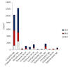
Figure 6.1: Zooplankton cell counts collected by vertical trawl measured in cells/m³ for 0845,0945 and 1045 for station 2

Figure 6.2 showed a larger abundance of phytoplankton at 7.00m than 1.00m. A greater number of species were seen to be present in deeper waters. Rhizosolenia alata, Rhizosolenia stegera, Rhizosolenia stolterfothii and Eucampala spp. were all observed at 7.00m but not 1.00m. Rhizosolenia setigera was the most abundant species with cell counts of 14 cells/mL.

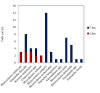
Figure 6.2: Phytoplankton cell counts in cells per ml at 1 and 7m sampled at Station 2 at 0845

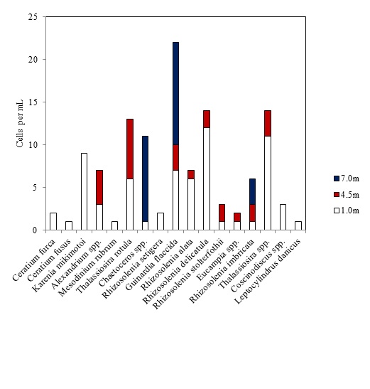
Figure 6.3 showed the greatest abundance of phytoplankton in the water column at 1.00m. Species diversity at 0945 was high. Guinardia flaccida, Thalassiosira spp. and Rhizosolenia delicatula were the most abundant species in the water column with more than 13 cells/mL. Guinardia flaccida and Rhizosolenia imbricata were present at all depths in the water column.

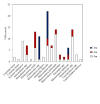
Figure 6.3: Phytoplankton cell counts in cells per ml at 1, 4.5 and 7m sampled at Station 2 at 0945

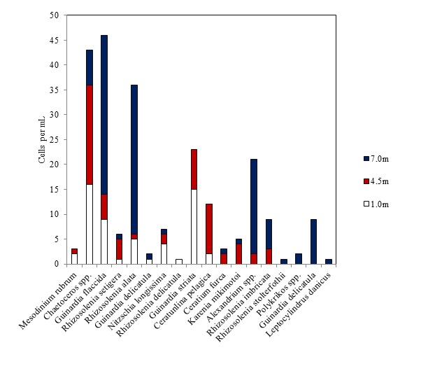
Figure 6.4 showed greatest abundance of phytoplankton at depths of 7.00m. Species variety was large across all depths of the water column. Guinardia flaccida was the most abundant species with over 45 cells/mL, and this species was present at all depths of the water column. At 7.00m there were three species with large observed cell counts, Alexandrium spp., Guinardia flaccida and Rhizosolenia alata.

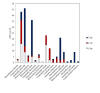
Figure 6.4: time series of chlorophyll (µg/l)  calulcate in the lab at station 2 between 0845 and 1045

The chlorophyll samples at Station 2 that were taken around 0.90m had a higher chlorophyll level than at 7.00m, but when samples were taken at intermediate depths such as at 0945 and 1045 there appeared to be a non-linear relationship with depth.  At 0945 there was a chlorophyll maximum with a value of 2.27 µg/l at 4.30m, whereas at 1045 there was a chlorophyll minimum of 1.65µg/l at 4.20m. At Station 2 there were fluctuations in chlorophyll concentration throughout the time series which appeared to exhibit no clear trend (Figure 6.5).

DISCUSSION

The tide was flooding the harbour for almost the entirety of the sampling period (high tide was at 1020, Table 2.1). This explains the layer of fresher water present in the top 1.20m until 0915. Because the tide was still flooding the estuary, freshwater still dominated the top layer and maintained a stratified system in the harbour. This was further supported by the temperature gradient at 0845 that exhibited a sharp drop at 1.30m, at almost exactly the same location as the halocline. As the morning progressed and more saline water entered the harbour, the stratification created by differing densities of fresh and salt water was broken down. This can be seen from 0945 until 1145 where temperature decreased steadily rather than exhibiting a sharp drop at 1.20m as seen at previous times. Even though high tide occurred at 1020, the direction of tidal currents had yet to change for sampling points 1045 onwards due a delay in the tidal height between the mouth of the estuary and the harbour. In all of the profiles there was an increase in salinity with depth and a decrease in temperature with depth. This is expected because the more saline, colder water flowing in from offshore is denser than the fresh-water inputs.

The breakdown of stratification over the course of the sampling period was further supported by the general increase in Ri number. As the morning progressed, the number of points in the water column where Richardson number exceeded 1.0000 increased. This indicates that the water column is unstable and encourages mixing of previously stratified layers.  This was further supported by the chlorophyll maximum present at 4.20m at 0945 (phytoplankton inhabited the waters just below the thermocline) whereas at 1045, there was a chlorophyll minimum at around the same depth. This shows that the stratification is beginning to break down and it is no longer beneficial for the plankton to concentrate themselves at this particular depth.

There was no particular trend spatially or temporally with respect to chlorophyll; this is consistent with our transmission and fluorescence data and is due to enough light and nutrients being available over the entire water column for the phytoplankton to use. However, in order to make a definitive conclusion, more data must be acquired. It can be assumed that any variation in transmission, chlorophyll and fluorescence data was due to small scale temporal and spatial changes in currents and nutrient availability.

The harbour in which we conducted the time series has a flushing time of around 2.4hours (IST and Falmouth Harbour Commissions, 2012). This leads to extremely regular replenishment of nutrients to support high levels of phytoplankton. By looking at our data, a decline in the concentrations of nutrients and dissolved oxygen with depth is evident,  indicating an uptake of these nutrients by plankton deeper in the water column.

The overall number of zooplankton species increased over the course of the day. This is due to more nutrient rich, salt water flooding the harbour and because light levels increase as we approach noon. This is supported by a depletion of oxygen and nutrients over the course of the day as numbers of respiring plankton rise. Both light levels and high nutrient concentrations in the water column contribute to more phytoplankton and therefore, more for the zooplankton to consume.

DISCUSSION OF OFFSHORE PRACTICAL

ESTUARINE PRACTICAL - Bio - Physical - Chemical - Summary - Back to top

INTRODUCTION

How does the estuary behave as a transition zone between the freshwater riverine and ocean environments?

Due to the enclosed nature of estuaries, their properties with respect to nutrient concentrations, oxygen availability, plankton abundance and light attenuation sometimes vary wildly. They tend to differ from the conditions found in both saline and riverine environments and do so in a graded manner over short spatial scales. Furthermore, they are often home to abnormal build-ups of pollutants. Our objective is to sample over a range of salinities whilst travelling down the estuary in order to observe these changes and make conclusions based on the results collected.

FIELD METHODS

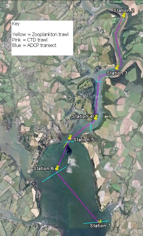
Fieldwork was carried out on the 3rd of July 2012, aboard the RV Bill Conway. Figure 7.1 shows a map of sampling stations and routes taken on the day, and exact positions are recorded in table 7.1. Times of high and low tides are displayed in table 7.2, along with local weather information and depths of the water column. At each station, CTD profiles and water samples at different depths were taken, ADCP transects across the estuary at each station were also recorded. When leaving Stations 2, 5 and 7, zooplankton trawls (using a 45.8cm diameter net) were carried out for 5 minutes and the volume of water flowing through the net was measured by a revolving flow meter. The CTD available did not have Niskin bottles attached therefore; water samples could only be taken using a hydroline and messenger system. This meant that samples were limited to 9m depth. Sampling was limited by the number of lugols bottles (for phytoplankton) and oxygen bottles we had available as there were only 5 bottles filled with lugols iodine available, and so decided to use two at Station 2, two at Station 4, and one at Station 7. There were sixteen oxygen bottles available, out of which five were used at Station 5 as this was a specific site of interest. Underway water samples (pumped on board from the surface of the water column) were collected at increasing salinity values whilst travelling between stations with the intention to measure dissolved silicon, chlorophyll and nitrate concentrations later on in the lab. The temperature, salinity, latitude and longitude were also recorded for each corresponding underway sample.

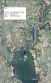
Figure 7.1: map of sampling stations and transects of the estuarine survey taken on 03/07/2012

Date: 3/07/2012

Figure 7.2

LAB METHODS

Samples were prepared in the wet lab ready for on-shore lab analysis as stated in the “Wet Lab Methods”

Physical - CTD data was managed and graphed using ‘Sigmaplot’. All Salinity data taken from the CTD had to be multiplied by 0.95 due to calibration issues. ADCP data was displayed using Winriver.

Chemical - Samples collected were analysed to quantify dissolved silicon, dissolved oxygen, chlorophyll and, nitrate and phosphate. Methods of analysis are stated in “Lab Methods”.

Biological - Both zooplankton and phytoplankton species were identified and counted. The exact method is stated in “Lab Methods”.

PHYSICAL RESULTS OF ESTUARINE PRACTICAL

ADCP

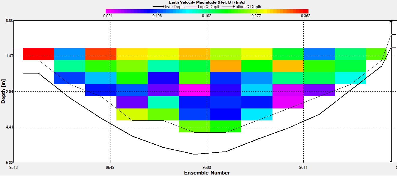
STATION 2

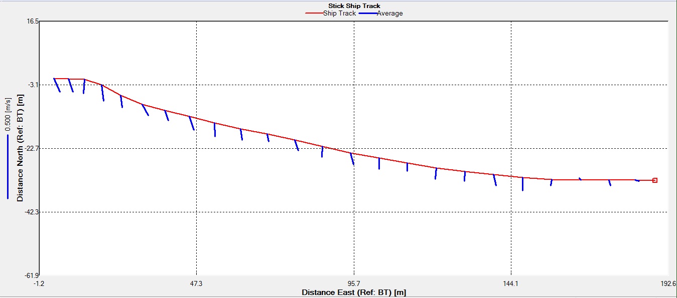
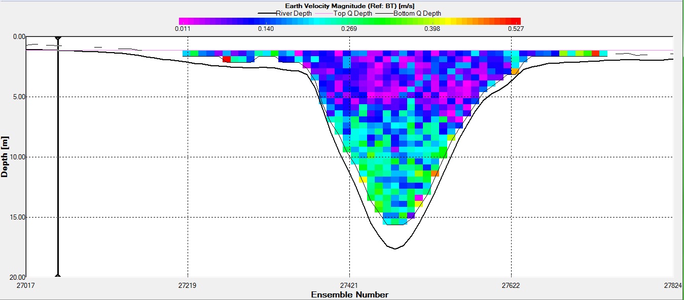
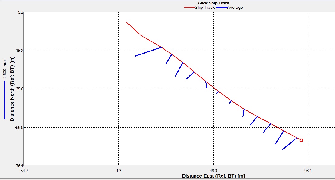
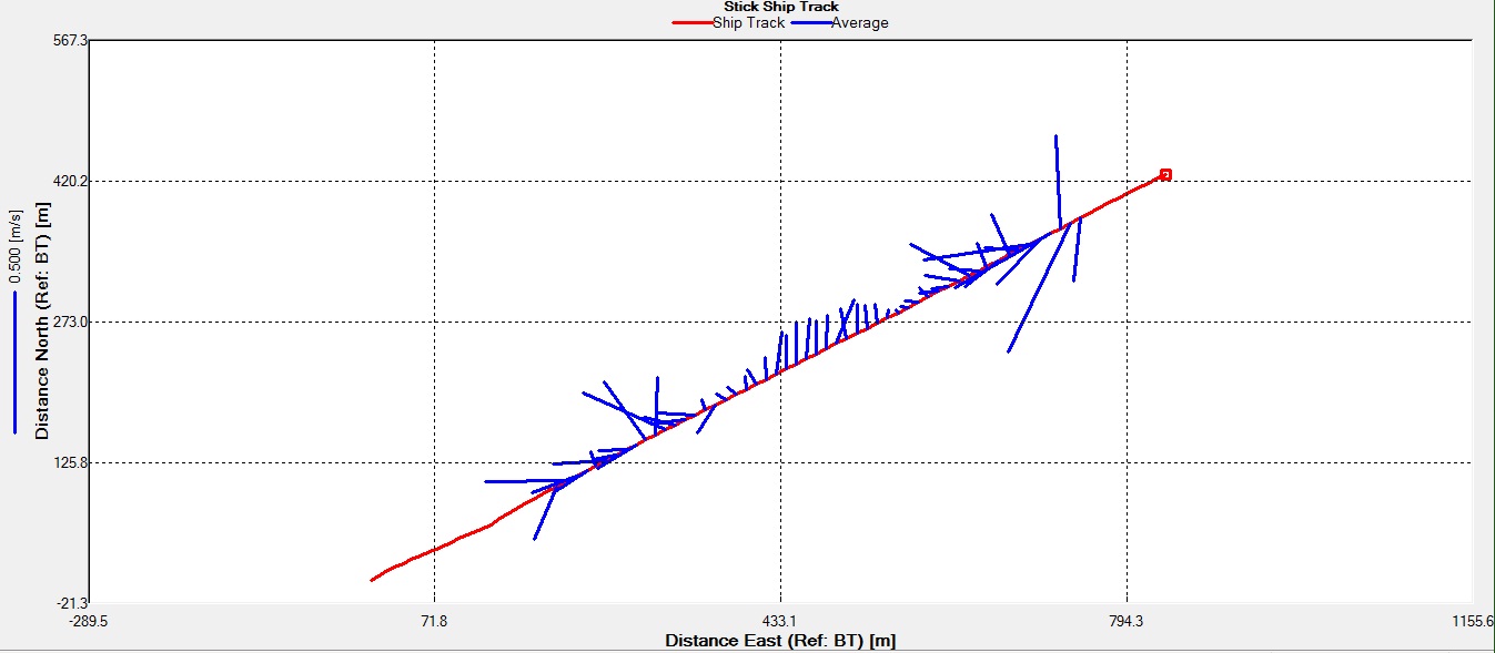
Maximum velocities were reached in the surface waters above 1.89m (Figure 8.1), with a maximum velocity of 0.362ms^-1 in the far west of the estuary. Velocities decreased with depth, minimum velocity was at 2.89m at 0.021 ms^-1. From the stick ship track, the dominant flow observed was south westerly, with a maximum velocity of 0.275 ms^-1(Figure 8.2).

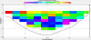
Figure 8.1 ADCP flow rate profiles (m/s) for station 2 taken at 0908

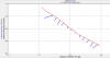
Figure 8.2: ADCP ship track for station 2 taken at 0908

STATION 3

The maximum flow velocity was found in the surface waters at the centre of the channel at 0.398 ms^-1(Figure 8.3). In the centre of the channel, velocity of the surface waters above 5m was greater than velocity of the water below 5m.  The minimum velocity recorded was 0.004 ms^-1 at 7.39m. The surface flow either side of the main channel was considerably lower than the surface flow in the channel.  The shallow waters to the west of the velocity plot, flow was low with no velocities recorded above 0.200 ms^-1.  The velocities on the eastern side of the transect regularly reached  velocities of over 0.200 ms-1 with a maximum velocity of 0.246 ms^-1. The stick ship track plot indicated weak southerly flows with no velocities over 0.15ms^-1(Figure 8.4).

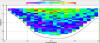
Figure 8.3 ADCP flow rate profiles (m/s) taken for Station 3 at 1009

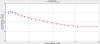
Figure 8.4: ADCP ship track for Station 3 taken at 1009

STATION 4

The maximum flow velocities were found within the centre of the channel up to 0.304 ms^-1 (Figure 8.5). Waters either side of the channel were found to have lower velocities.  Generally, velocities increased towards the centre of the plot. Velocities did not vary with depth. The stick ship track plot showed an easterly flow direction with a maximum velocity of 0.124 ms^-1 (Figure 8.6).

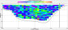
Figure 8.5: ADCP flow rate profiles (m/s) at Station 4 at 1054

Figure 8.6: ADCP ship track for Station 4 at 1054

STATION 5

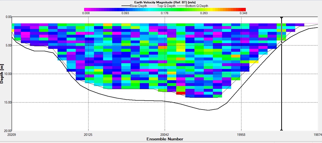
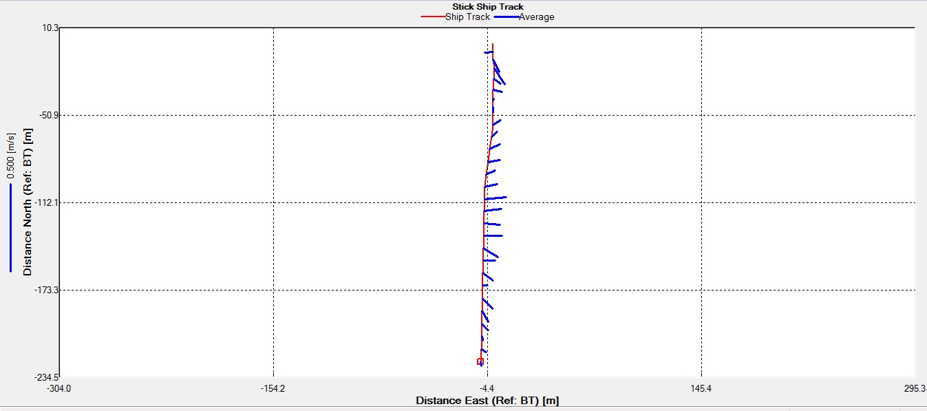
Low velocities were consistently observed throughout the water column. The eastern side of the transect showed slightly greater velocities reaching up to 0.447 ms^-1 at 1.39m(Figure 8.7). However, the far west of the transect showed a maximum velocity of 0.250 ms-1.The centre of the channel showed no significant variation with depth. However, the four largets velocities (0.24 ms^-1 ,0.241 ms^-1 ,0.268 ms^-1 ,0.248 ms^-1) were found between 4.89m and 9.89m. From the stick ship track plot  a northerly flow was observed, with greatest velocities towards the east of the channel which reached 0.447 ms^-1 (Figure 8.8). Some eddying was present in the far west of the channel, with a velocity of 0.121 ms^-1 flowing southwards.

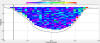
Figure 8.7: ADCP flow rate profiles (m/s) taken at Station 5 at 1119

Figure 8.8 ADCP ship track for Station 5 at 1119

STATION 6

In the surface waters the velocities were greater either side of the channel than the centre of the channel.  Within the centre of the channel, below a depth of 6.89m, a large area of high velocities was seen to extend down to the bottom of the water column with a maximum velocity of 0.47 ms^-1 (Figure 8.9).  In water shallower than 6.89m, in the centre of the channel, the greatest velocity recorded was 0.25 ms^-1. The flow in the centre of the channel was slow and northerly (Figure 8.10).

Figure 8.9: ADCP flow rate profiles (m/s) for Station 6 at 1212

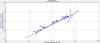
Figure 8.10 ADCP ship track for Station 6 at 1212

STATION 7

Interpretation of data from station 7 has been omitted, due to the depth of the channel being too great for the ADCP to accurately determine the velocities present in the water column.

RICHARDSON NUMBER

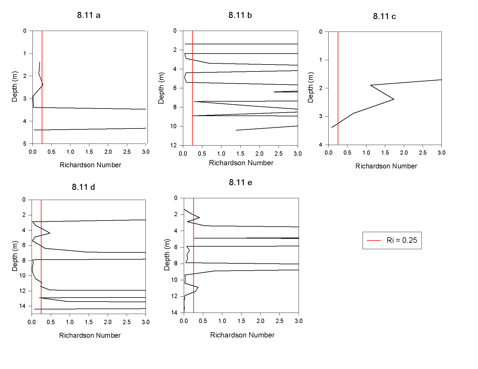
Figure 8.11: Richardson numbers for estuary stations, red line where Ri=0.25, a=station 2, b=3, c=4, d=5, e=6

In the top 6m at station 3 (Figure 8.11b), Richardson number readily fluctuated above and below 0.2500. However at depths greater than 6m, Richardson number was only lower than 0.2500 at one depth, 8.89m.

Richardson number at station 4 (Figure 8.11c) was greater than 0.2500 at the majority of depths.

Station 5 (Figure 8.11d) shows a region of the water column, between 2.89m and 11.89m where Richardson number is predominantly below 0.2500. However, Richardson number was above 0.2500 between 3.89m to 4.39m and ,6.89m to 7.39m. Below 11.89m, Ri was lower than 0.25 at two depths, 12.89m and 14.39m.

The station 6 depth profile (Figure 8.11) showed 3 main regions where Ri was lower than 0.25. The first of these was the surface waters down to a depth of 3.39m, here the Ri was greater than 0.2500 for only a small period at 2.39m.  The second of these regions was from 5.89m to 7.89m, where Richardson number was consistently lower than 0.2500. Richardson number increased above 0.2500 until 9.39m where it remained below 0.2500 for a further meter. The final region where Ri was lower than 0.2500, was from 11.89m to the maximum depth, where Ri was permanently below 0.25. 

CTD

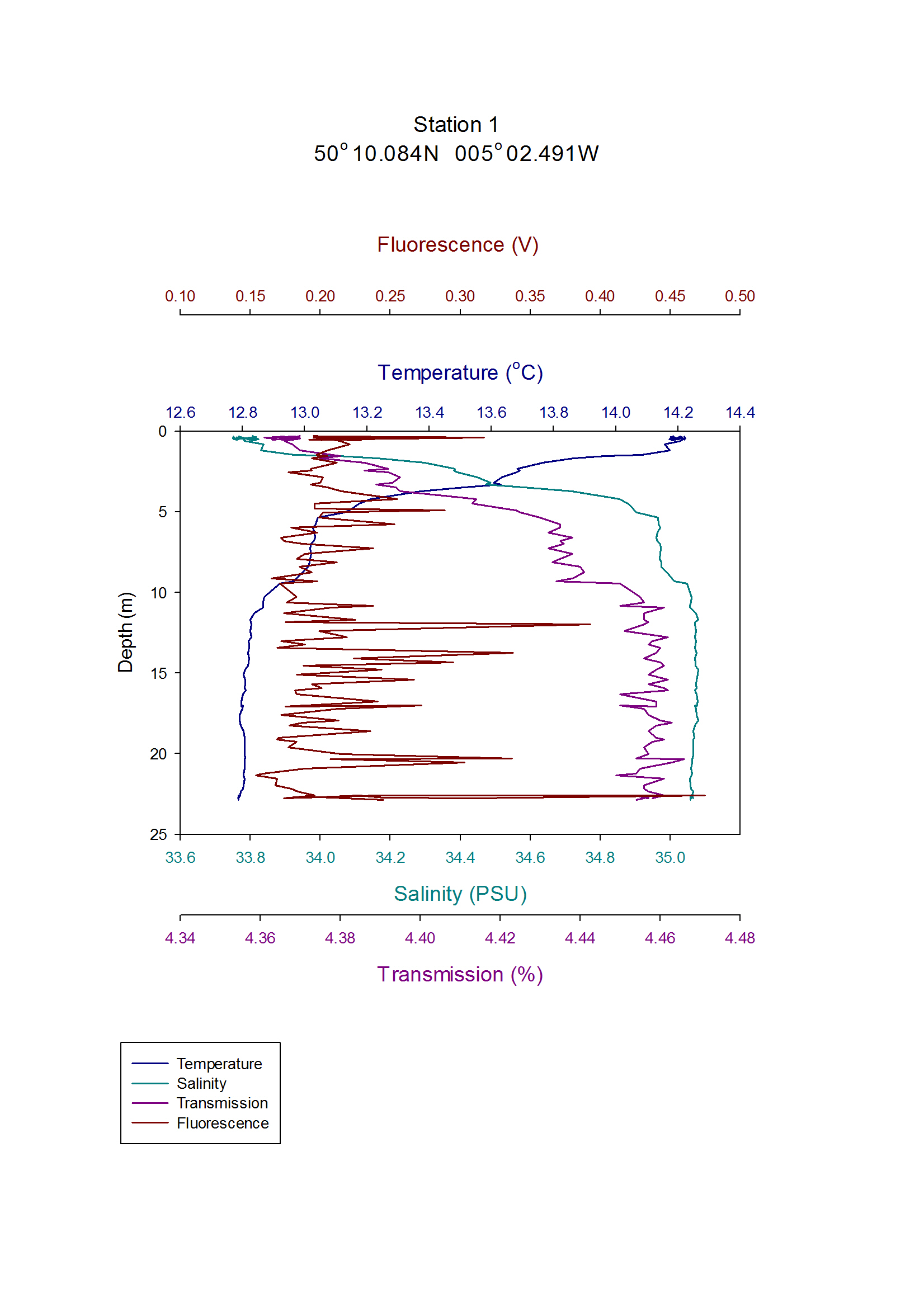
Figure 8.12 shows CTD data for station 1. The temperature was 14.18^oC at an uppermost depth of 0.40m. This decreased steadily to 13.04^oC by 5.34m depth. The temperature remained constant from 5.34m to 8.12m at around 13.02^oC, before it decreased to 12.80^oC by 11.26m, and remained near this value for the rest of the water column. Salinity increased steadily from 33.77 at the surface to 34.97 at 5.34m depth. The salinity remained at 34.97 until 8.39m depth. By 9.45m, salinity increased to 35.05, and stayed near this value for the remainder of the profile. Transmission, whilst fluctuating, increased from 4.35% at the surface to 4.45% by 11.26m, where it remained fluctuating around this value with increasing depth. Fluorescence fluctuated widely throughout the whole profile, generally about 0.21 mg/m^-3, ranging from 0.15 to 0.43 mg/m^-3.  The two biggest peaks occurred at 12.06m and 22.69m, with values of 0.48 and 0.39 mg/m^-3 respectively.

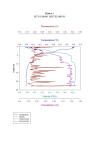
Figure 8.12: CTD data measuring temperature (⁰C), fluorescence (V), salinity and transmission (%) measured at Station 1

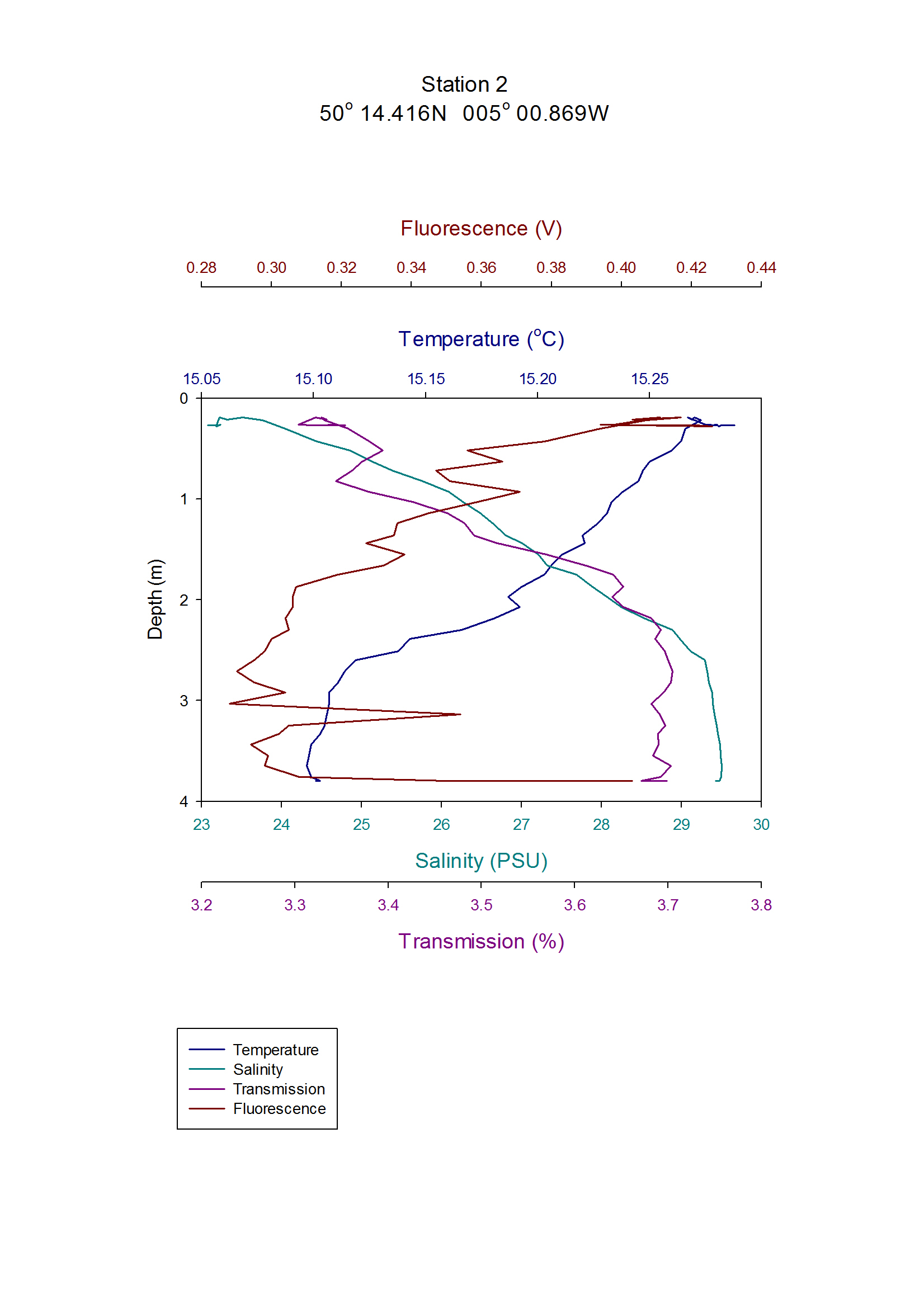
The temperature of the column at station 2 (figure 8.13) decreased steadily from 15.26^oC to 15.11^oC in the surface 2.92m, as shown in figure 2. For the remainder of the profile to a depth of 3.80m the temperature remained close to 15.10^oC. Salinity increased from 23.22 to 29.29 from the surface to 2.60m. Beyond this depth, salinity values remained fairly constant at 29.4. Fluorescence decreased from 0.42V at the surface to 0.29V at 2.71m depth, and exhibited fluctuations. Below this depth, values remained close to 0.29V, with the exception of a peak of 0.35V at 3.15m and 0.40V at 3.80m. As a general trend, transmission increased from 3.33% to 3.69% from the surface to 2.23m depth, with the exception of increasing to 3.39% at a depth of 0.52m.  Values remained close to 3.69% for the remainder of the profile.

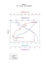
Figure 8.13: CTD data measuring temperature (⁰C), fluorescence (V), salinity and transmission (%) measured at Station 2 at 0945

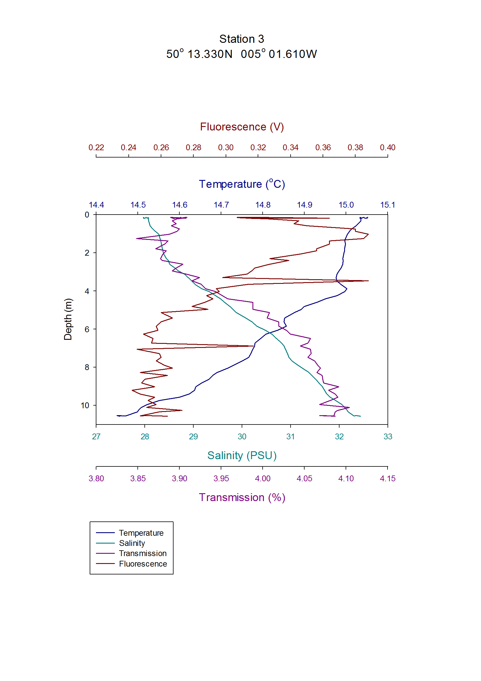
Figure 8.14 shows the CTD profile for station 3. There was a temperature of 15.05 ^oC at the surface, this dropped gradually to around 15.00 ^oC at 4.03m then decreased steadily from there to around 14.46 ^oC at 10.56m. Salinity increased steadily as depth increased starting at 27.97 at the surface and then rose to 32.44 at 10.56m. Transmission dropped from around 3.91% at the surface to 3.90% at 0.16m. It then increases steadily with depth and reached a maximum of 4.10% at 10.10m. Transmission followed the same pattern as salinity, however, a small fluctuation existed where rate of transmission rose from 3.94% at 4.03m to 4.01% at 5.12m. Fluorescence exhibited a decline with increasing depth. The surface fluorescence was around 0.32V and showed a sharp increase to 0.39V at 1.02m. This then declined steadily to 0.26V at 6.06 m, it remained at this approximate voltage for the remainder of the water column. Sharp peaks were present at 3.47m and at 6.88m to 0.39V and 0.32V respectively.

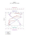
Figure 8.14: CTD data measuring temperature (⁰C), fluorescence (V), salinity and transmission (%) measured at Station 3 at 1020

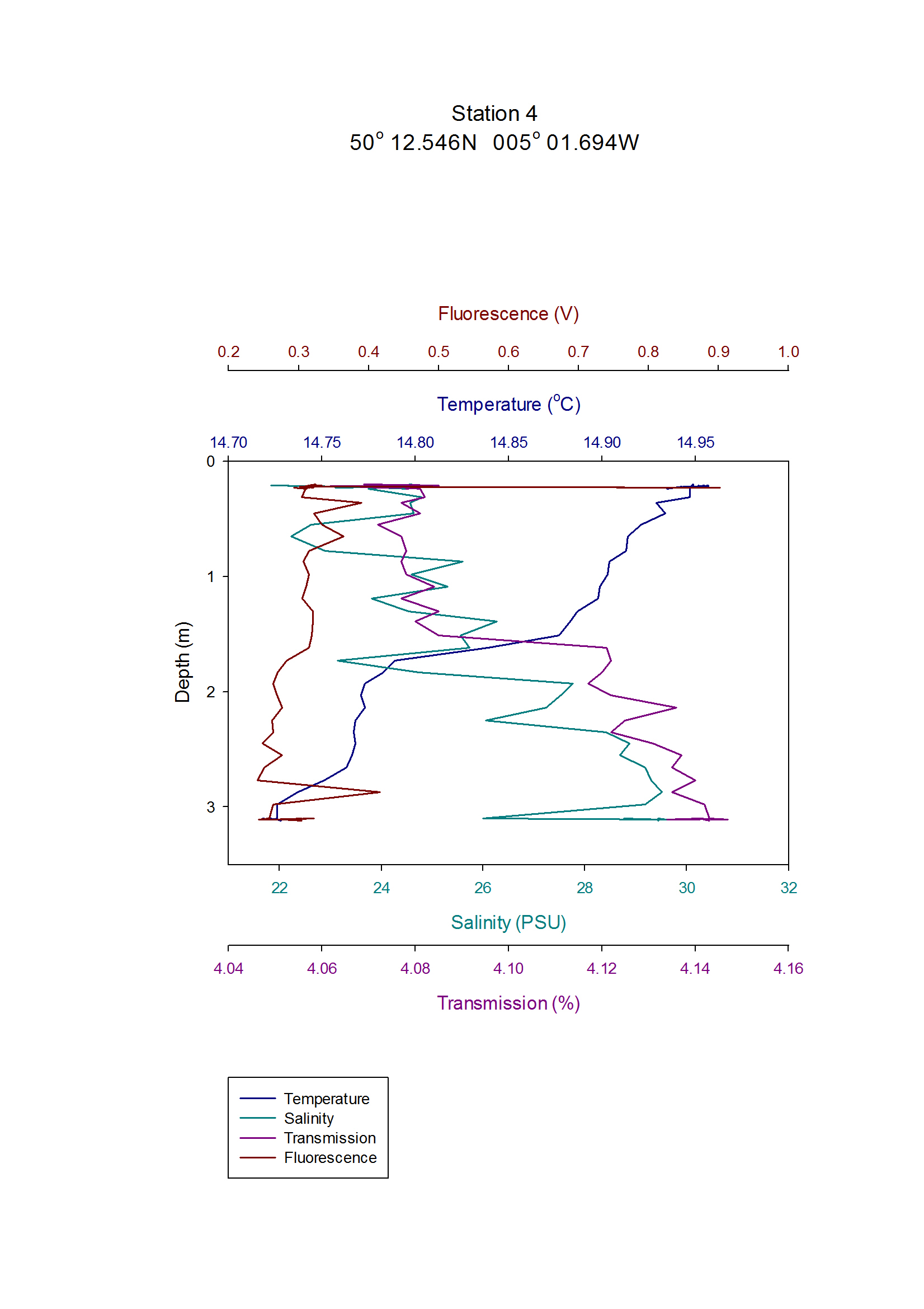
Figure 8.15, displaying data for Station 4, showed a general increase in salinity from 21.83 to 29.00 over the whole 3.11m profile, which fluctuated widely compared to other profiles. Temperature decreased steadily from 14.95^oC at the surface to 14.88^oC at 1.51m depth.  This was followed by a more rapid decrease in temperature to 14.79^oC  by 1.73m depth. The decrease in temperature then slowed, reaching 14.76^oC by 2.66m depth, before decreasing more rapidly again to 14.72^oC at 3.10m depth. Omitting two large peaks in fluorescence, one at the very surface (at 0.90V) and a peak of 0.42V at 0287m, fluorescence remained between 0.24V and 0.39V for the whole profile, decreasing gradually throughout. Transmission values were between 4.07% and 4.08% for the top 1.51m of the water column, before increasing rapidly to 4.12% by 1.62m. Below which, transmission increased gradually to 4.15% at 3.11m depth with values fluctuating slightly.

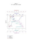
Figure 8.15: CTD data measuring temperature (⁰C), fluorescence (V), salinity and transmission (%) measured at Station 4 at 1104

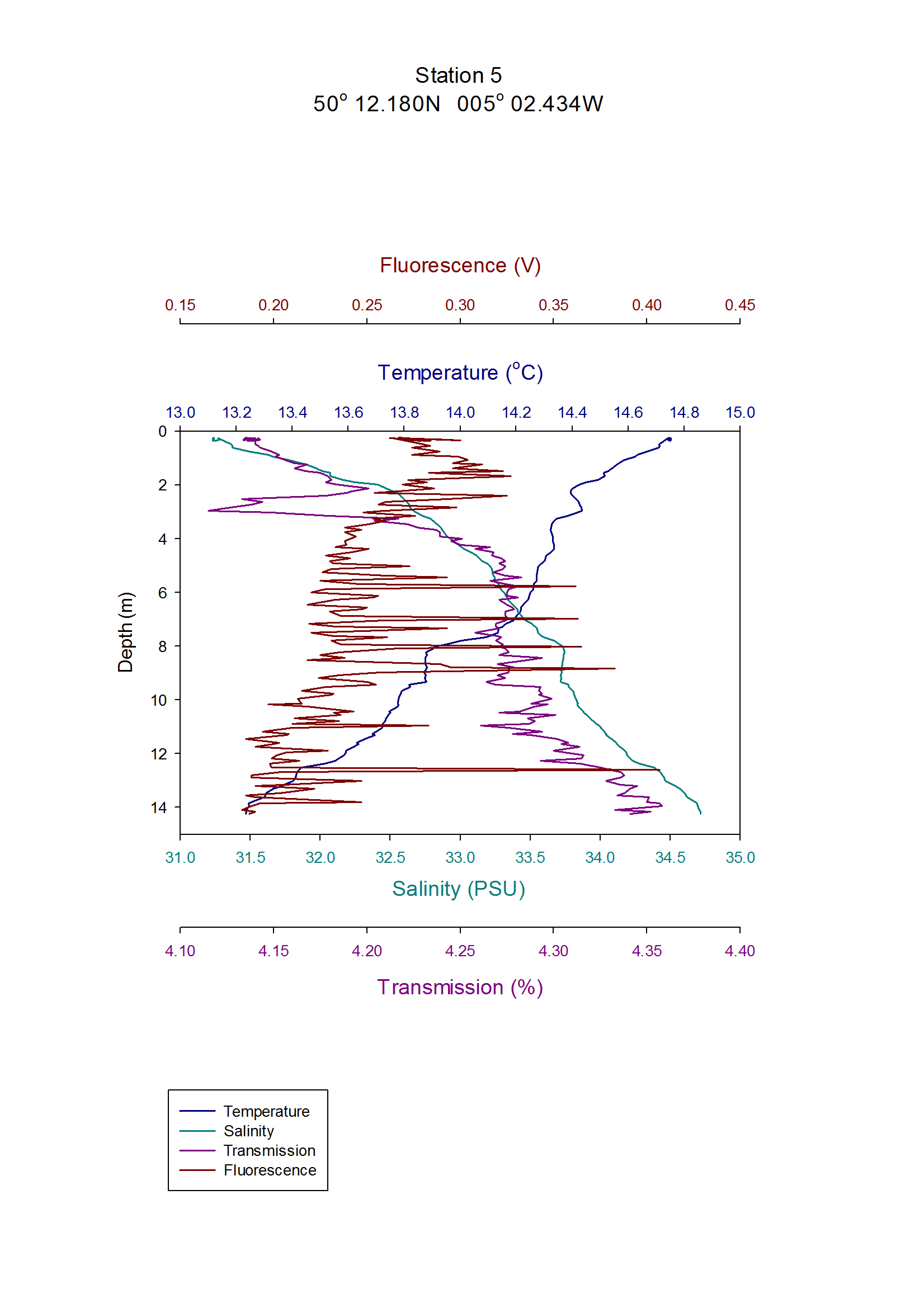
Temperature declined steadily with depth from 14.75 ^oC at the surface to 13.23 ^oC at 14.24m at station 5, as shown in Figure 8.16. Salinity, on the other hand displayed a steady increase with depth from 33.83 at the surface to 34.72 at 14.24m. The rate of increase in salinity was slightly quicker in the top 2m of the water column. Fluorescence, showed large fluctuations throughout the water column, particularly under 4m where there were peaks of 0.41V, 0.38V and 0.37V at 12.59 m, 8.83m and 8.01m respectively. Larger peaks in fluorescence occurred deeper, despite these peaks a general decline in fluorescence with depth was seen from 0.29V at 0.30m to 0.18V at 14.10 m, it then exhibited a rise as water depth increased, this increase was rapid between 0.30m and 2.13m where transmission rose from 4.14% to 4.20%. A sharp decline in transmission was seen at 2.96m to 4.12%. It increased rapidly between 2.96m and 5.02m from 4.12% to 4.27% where it remained until 9.42m, transmission then increased gradually to 4.35% at 14.16m.

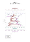
Figure 8.16: CTD data measuring temperature (⁰C), fluorescence (V), salinity and transmission (%) measured at Station 5 at 1143

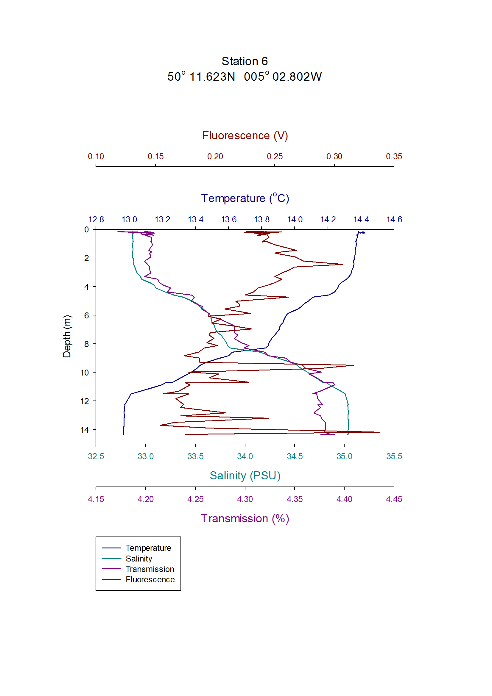
Data for station 6 is displayed in Figure 8.17. Temperature was 14.39 ^oC at the surface and remained relatively constant until 4.07m where there was a sudden decrease to 14.08 ^oC at 5.01m. This then decreased steadily to 13.82 ^oC at 8.29m and then rapidly to 13.01^oC at 11.50m. Temperature remained at this approximate level as depth increased. Salinity increased with depth. It remained at around 32.87 until 2.62m then rose to 33.85 at 8.29m. A rapid increase to 35.00 at 11.49m then occurred, and remained relatively constant for the rest of the water column. Fluorescence fluctuated greatly between around 0.15V and 0.30V, however, a slight decline with depth was present with fluorescences of 0.23V at 0.21m and 0.19V at 13.98m. Transmission followed the same pattern as salinity with two rapid increases in % transmission at around 5m and 10.5m from 4.21% at 3.47m to 4.26% at 5.87m, then, from 4.36% at 10.09m to 4.40% at 10.87m. Transmission then remained at approximately 4.40% from 10.87m to 14.35m. 

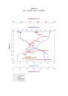
Figure 8.17: CTD data measuring temperature (⁰C), fluorescence (V), salinity and transmission (%) measured at Station 6 at 1157

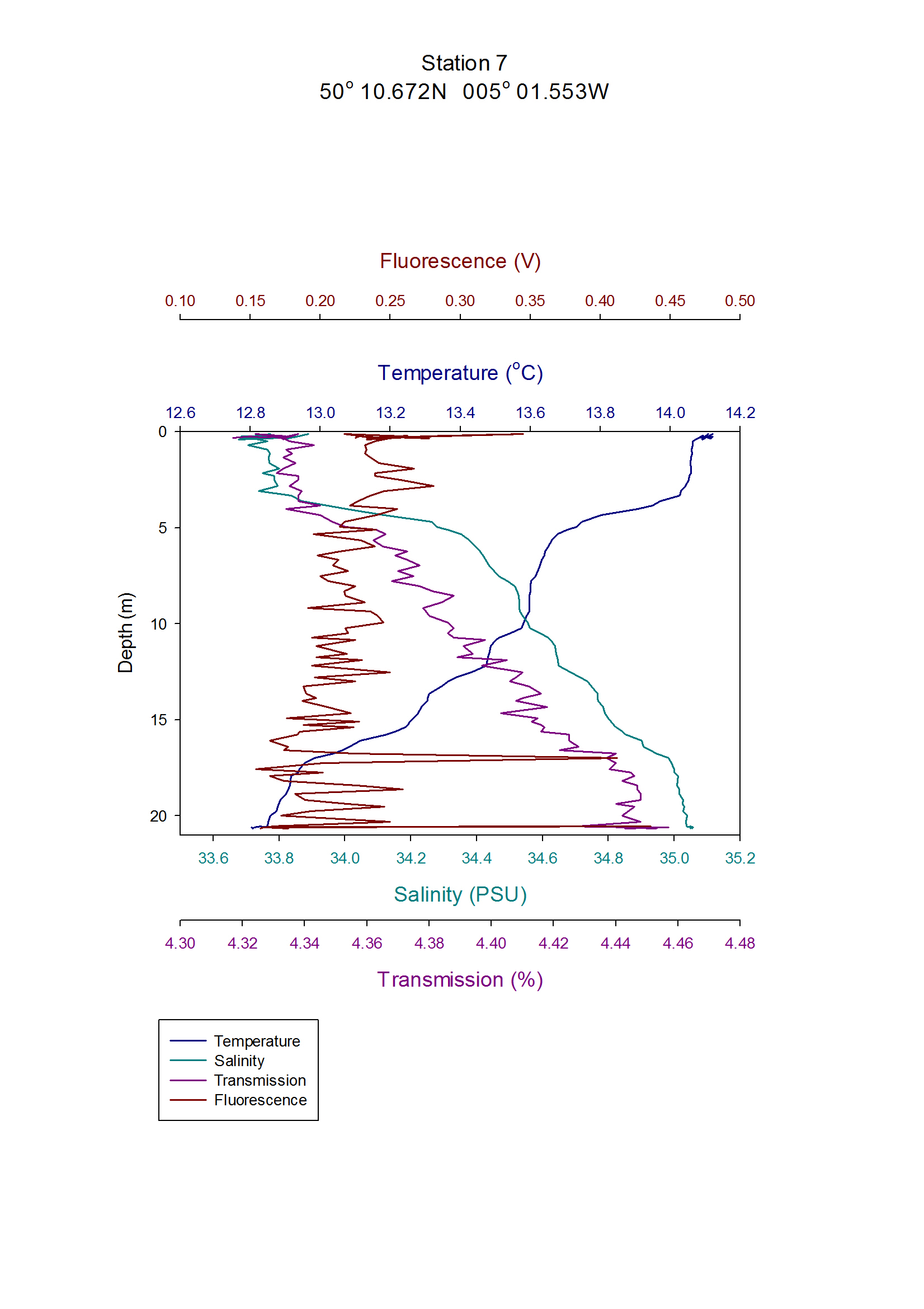
The temperature at station 7 (Figure 8.18) declined from 14.11 ^oC to 12.81 ^oC from the surface to 20.67m. A sharp decrease in temperature was seen between 3.33m and 5.98m from 14.03 ^oC to 13.63 ^oC. Salinity remained steady around 33.75 from the surface to 3.84 m, a rapid increase then occured to 34.41 at 4.35m. Salinity rose steadily for the remainder of the water column until a maximum of 35.04 at 20.67m. Transmission remained constant around 4.33% until a depth of 4.6m where it then increased rapidly to 4.37% at 6.23m. A steady decline in % transmission with minor fluctuations then occurred until a minimum value of 4.42% was reached at 20.55m. Fluorescence declined slightly over the entire water column from around 0.25V at the surface to 0.16V at 20.67m. As also seen at Station 5, we saw large peaks in fluorescence at depth. These occurred at 20.55m and 16.99m with voltages of 0.44V and 0.41V respectively, both of these values were larger than any other in the entire water column.

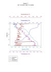
Figure 8.18 CTD data measuring temperature (⁰C), fluorescence (V), salinity and transmission (%) measured at Station 7 at 1233

CHEMICAL RESULTS OF ESTUARINE PRACTICAL

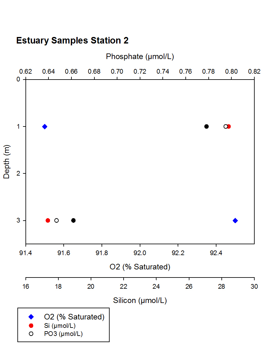
At Station 2 of the estuarine sample set (Figure 9.1), data was recorded from 1m and 3m depths. Between depths of 1 to 3m oxygen saturation percentages only increased by 1 per cent, from 91% to 92%. Dissolved silicon levels decreased over the depths, from 28.43µmol/l to 17.36µmol/l. Phosphate levels showed a relative decrease of 0.149µmol/l, from 0.795µmol/l to 0.647µmol/l over the depth increase.

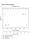
Figure 9.1: Phospohate (µmol/L), Silicon (µmol/L) and 02 (% saturation) profiles at Station 2 at 0945

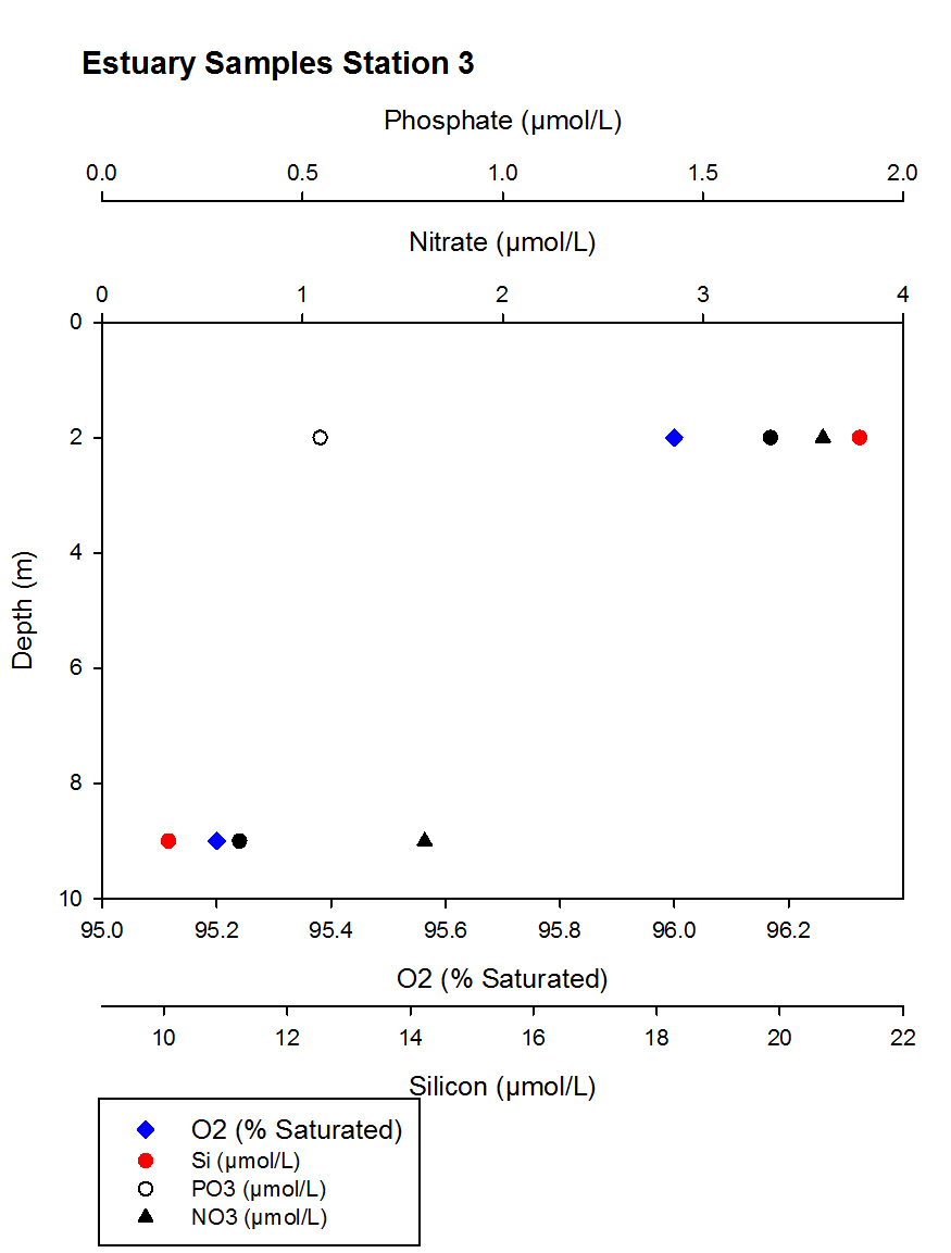
At Station 3 of the estuarine sample set (Figure 9.2), data was recorded from 2 different depths, 2m and 9m. Oxygen saturation percentages decreased over the depth change from 96% to 95% saturated. Dissolved silicon and nitrate levels also decreased from 21.29µmol/l to 10.08µmol/l and 3.60µmol/l to 1.61µmol/l consecutively. Only one result for Phosphate could be recorded due to low levels of sample solution. The single Phosphate sample showed a value of 0.544µmol/l.

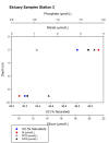
Figure 9.2: Phospohate (µmol/L), Silicon (µmol/L) and Nitrate (µmol/L)  and 02 (% saturation) profiles at Station 3 at 1020

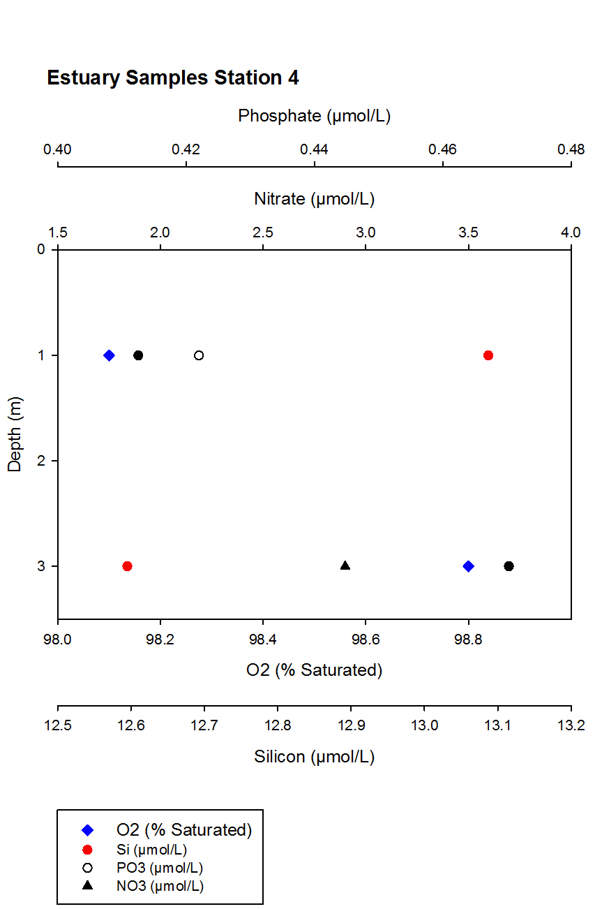
At Station 4 of the estuarine sample set (Figure 9.3), data was recorded from 2 different depths, 1m and 3m. Oxygen saturation percentage values did not change between these depths. Dissolved silicon levels decreased from 13.09µmol/l to 12.60µmol/l with the decrease in depth. Both phosphate and nitrate levels only have single data points due to lack of low levels of sample solution and limited laboratory equipment.

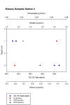
Figure 9.3: Phospohate (µmol/L), Silicon (µmol/L) and Nitrate (µmol/L)  and 02 (% saturation) profiles at Station 4 at 1104

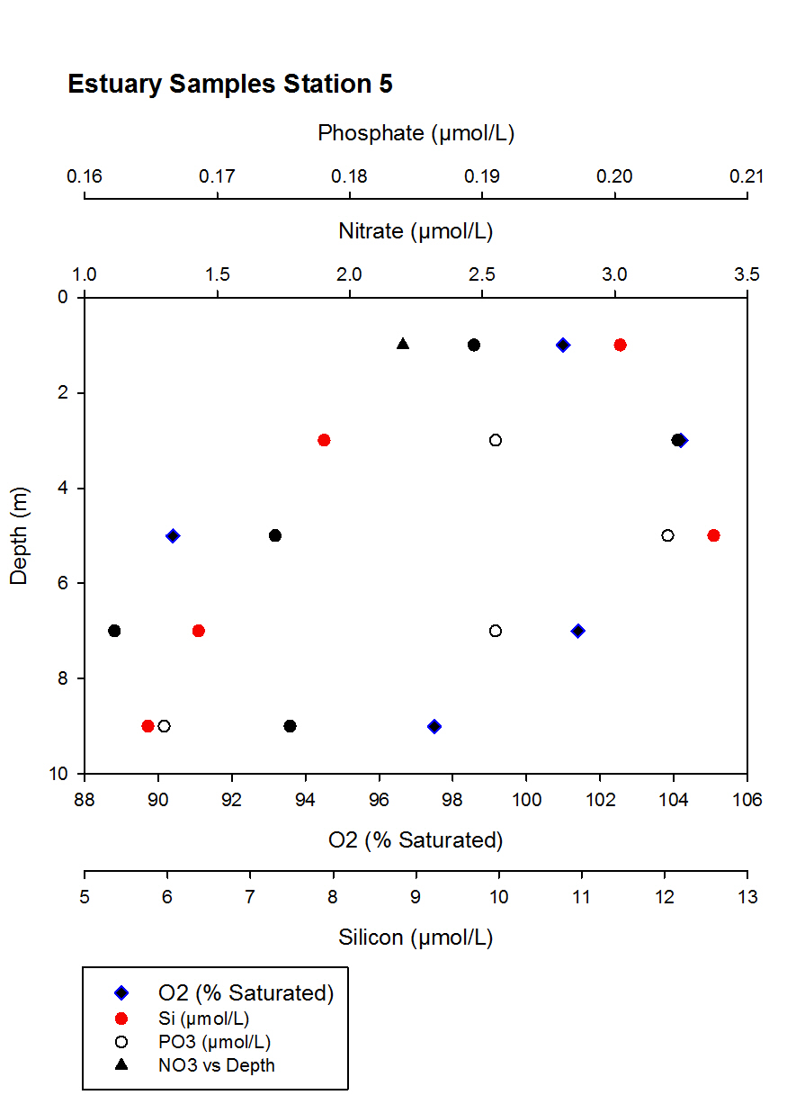
At Station 5 of the estuarine sample set (Figure 9.4), data was recorded from 5 different depths, 1, 3, 5, 7 and 9m. A slight increase in oxygen saturation was seen from 1m to 3m from 101% to 104%, and then an intermediate drop was recorded at 5m to 90% saturated. At 7m another increase in oxygen saturation was recorded at 101% which decreased to 97% at 9m. Dissolved silicon levels followed a similar pattern to oxygen levels, however an increase was recorded from 11.47µmol/l to 7.89µmol/l at depths of 1m and 3m. Dissolved silicon levels then increased to 12.60µmol/l at 5m and dropped down to 6.37µmol/l and 5.77µmol/l at 7m and 9m consecutively. Phosphate levels were recorded for 3, 5, 7 and 9m. Phosphate concentration increased from 0.191µmol/l to 0.204µmol/l at depths of 3 and 5m and then decreased to 0.191µmol/l and 0.166µmol/l depths of 7 and 9m. Only one sample of nitrate was processed at this station at a depth of 1 metre, the value recorded was 2.20µmol/l.

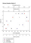
Figure 9.4: Phospohate (µmol/L), Silicon (µmol/L) and Nitrate (µmol/L)  and 02 (% saturation) profiles at Station 5 at 11.43

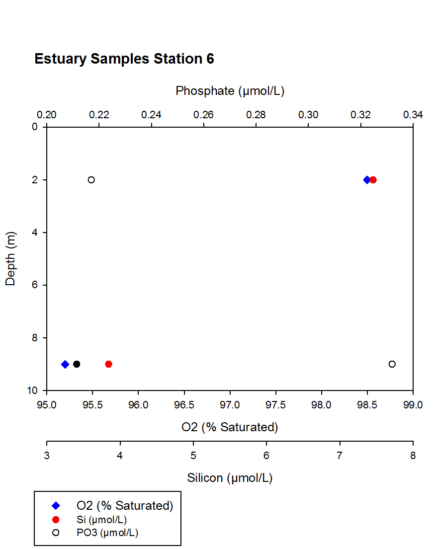
At Station 6 of the estuarine sample set (Figure 9.5), data was recorded from 2 different depths, 2m and 9m. Oxygen saturation percentage values decreased from 98% saturated to 95% saturated between the two depths. Dissolved silicon levels also decreased with increasing depths, from 7.45µmol/l to 3.85µmol/l. Phosphate increased relatively with an increase in depth, from 0.217µmol/l to 0.332µmol/l.

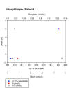
Figure 9.5: Phospohate (µmol/L), Silicon (µmol/L) and 02 (% saturation) profiles at Station 6 at 1157

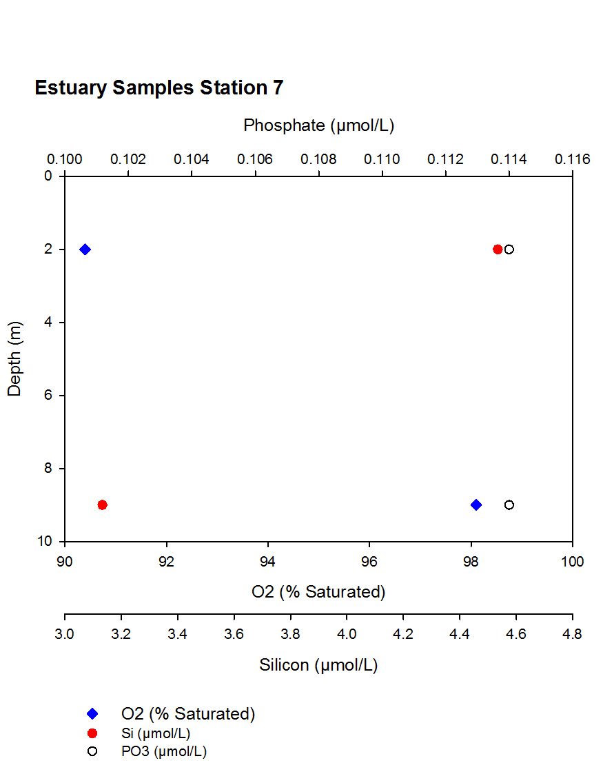
At Station 7 of the estuarine sample set (Figure 9.6), data was recorded from 2 different depths, 2m and 9m. Oxygen saturation percentage values increased from 90% to 98% saturated between 2 and 9m. Dissolved silicon concentrations decreased from 4.53µmol/l to 3.13µmol/l with the increase in water depth. Phosphate levels stayed current between the two depths at a concentration of 0.114µmol/l.

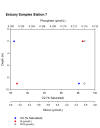
Figure 9.6: Phospohate (µmol/L), Silicon (µmol/L) and 02 (% saturation) profiles at Station 7 at 12.33

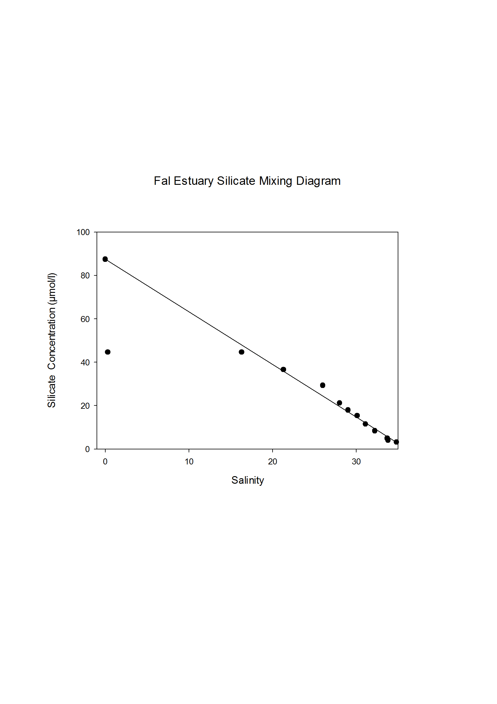
THEORETICAL DILUTION LINE

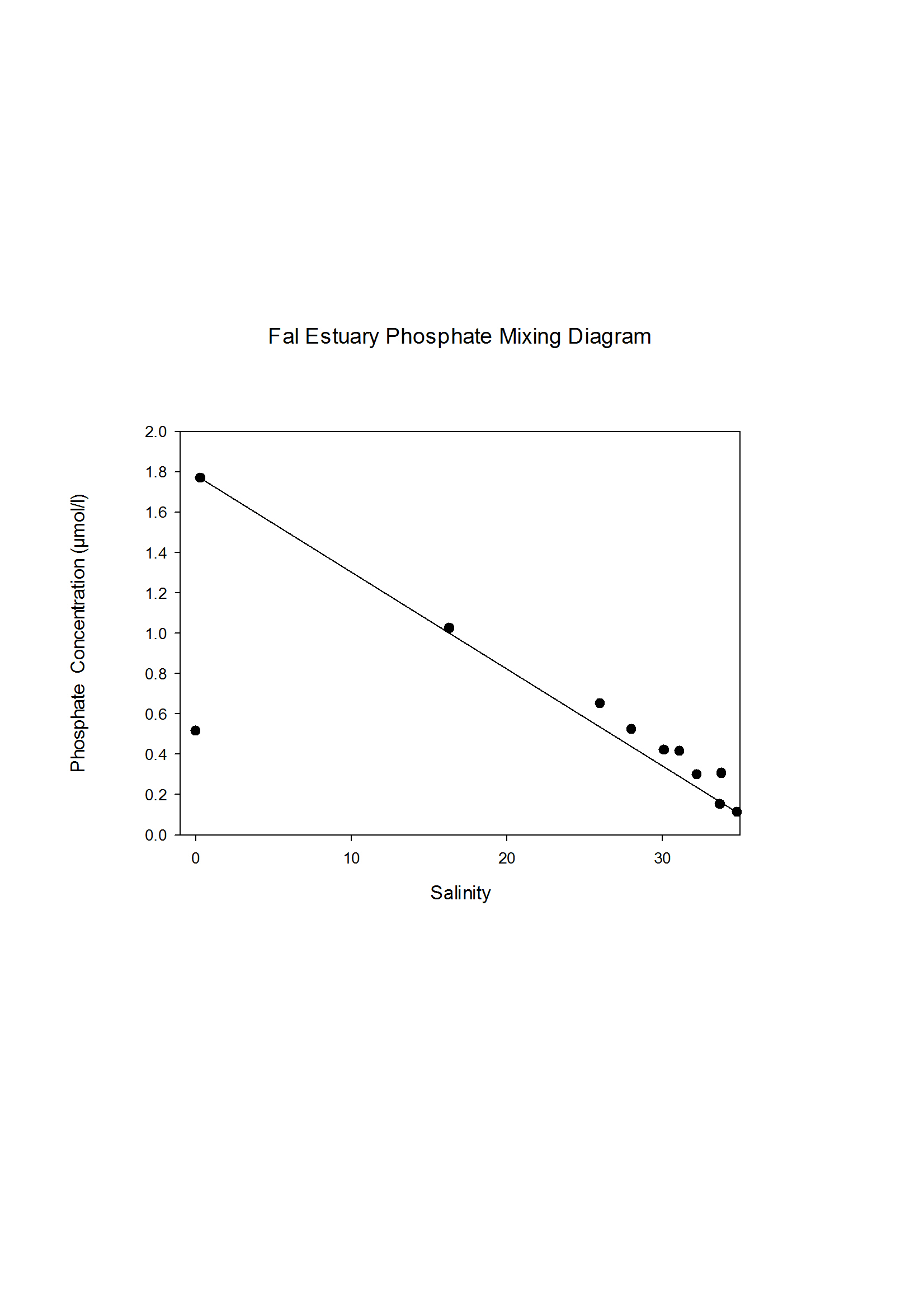
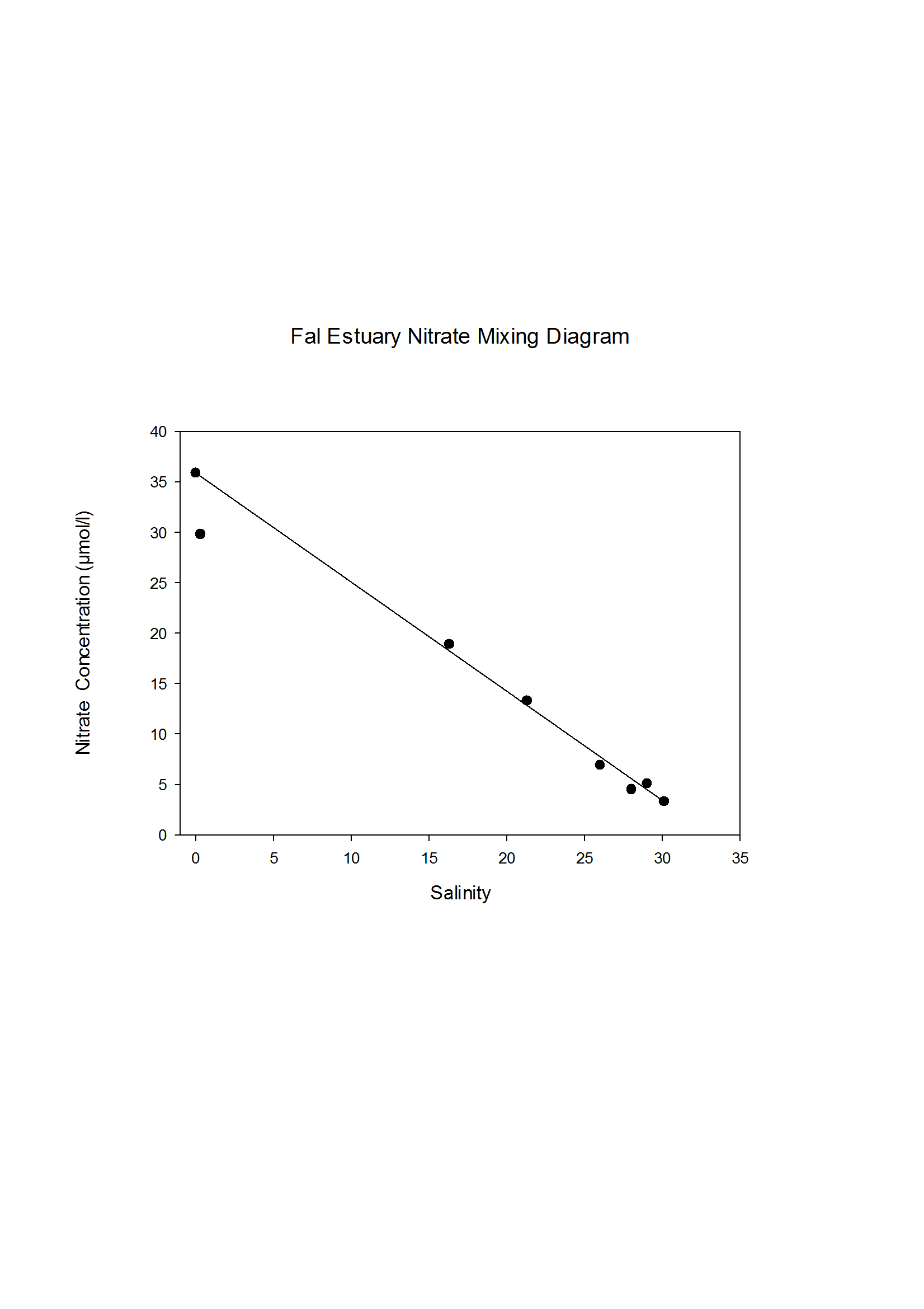
In Figures 9.7-9.9 the theoretical dilution line (TDL) joins the two end members. The seawater end member was obtained from the deepest sample (9.00m) at the last station (7) as this was the highest salinity sample collected;  with a salinity of 34.8 and silicate concentration of 3.13µmol/l (Figure 9.7) phosphate concentration of 0.140 µmol/l (Figure 9.8), and nitrate concentration of 3.31 µmol/l (Figure 9.9) . The river water end member was calculated by taking an average of the 3 nutrient concentrations;  87.50, 0.520 and 35.90 µm/l respectively (Figure 1-3) obtained from the River Allen and Kenwyn, both of which had 0 salinity.

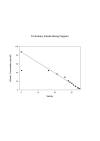
Figure 9.7: Estuarine mixing diagram showing Silicate concentration against salinity, the theoretical dilution line joins the 2 end members

Figure 9.8: Estuarine mixing diagram showing Phosphate concentration against salinity, the theoretical dilution line joins the 2 end members

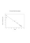
Figure 9.9: Estuarine mixing diagram showing Nitrate concentration against salinity, the theoretical dilution line joins the 2 end members

The silicate concentrations plotted on Figure 9.7 generally plot along the theoretical dilution line (TDL) between the salinity 28.0 and 34.8 towards the mouth of the estuary which is an indication of conservative behaviour however there are 3 points which fall either above or below the theoretical dilution line. A concentration of44.7 µm/l was calculated at a salinity of 0.3, which fell well below the TDL suggesting a net removal from the estuary, similarly to the concentration of 44.60 µm/l recorded at a salinity of 16.3, however this was only a slight deviation from the TDL. A silicate concentration of 29.30 µm/l plotted above the TDL suggesting a net gain of silicate.

In Figure 9.8 a negative correlation of increased salinity with decreased phosphate concentration decrease is shown. However, it appears that phosphate behaved non-conservatively, with values plotting well above the TDL at intermediate salinities. For example, at salinity 16.3 the nitrate concentration is 1.03 µm/l, suggesting that addition of phosphate is occurring.

The estuarine mixing diagram for the nitrate shown in Figure 9.9, showed a positive linear relationship between salinity and nitrate concentration, as an increase in salinity is reflected by an increase in nitrate. This relationship and the fact that the sample points plot along the TDL with little fluctuation indicates that only nitrate was behaving conservatively in the estuary, with little addition or removal occurring.

ESTUARINE RESIDENCE TIME

The residence time of the estuary was calculated using the equation below, and this was chosen rather than the tidal prism method because most of the stations were in the upper Fal estuary where tidal influences are less dominant.

Tres= ((1- Smean/Ssea)*Vtotal)/R

Where;

Tres= Residence time (s)

Smean= average salinity 

Ssea= Salinity of the sea

Vtotal=Total volume of the estuary (m3)

R=Riverine flux (m3s-1)

The average salinity of 28.84 was calculated using the underway sample data collected on 3/07/12 (between stations 2 and 5, which were the transects used to calculate volume) to ensure that the salinity values used to calculate the average were taken from the same depth along the estuary and the salinity of the sea 34.8 was taken at station 7 as this was approximately the salinity of the sea. The value of the riverine flux was taken from the Tregony-Fal data station operated by NERC (www.ceh.ac.uk/datanrfa/data/station.html). This station covers a catchment area of 87km2 and the mean flow 0f 2.028 m3s-1 is averaged over the period 1978-2010. The total volume of the estuary was calculated using both the ADCP data and Google Earth. The ADCP data was used to work out the cross sectional area of  the horizontal transects (Table 1) however we only used data from the transects 2,3,4 and 5 as 6 and 7 did not span the full width of the estuary therefore the data was incomplete. Google Earth was used to plot the horizontal transects taken at each station (Figure 1) and the distance between each transect was calculated, therefore the area could be calculated using the equation 1/3(a2 + ab + b2)h. The volume calculated of 7005522.83m3 is only a rough approximation as the calculation assumes that the estuary is straight and the channel depth increases at a constant rate. Due to the incomplete ADCP data the full volume of the estuary could not be calculated and so the residence time calculated may have been effected.

Tres=((1-28.84/34.8)*7005522.83)/2.028)=591615.6s = 6.85 days

It should be noted that the Riverine flux measured at Tregony station may not be a true representation of the Fal Estuary as it is located towards the upper Fal River, a great distance from where the samples were taken and the River Fal is also not the only freshwater input into the estuary. Secondly the R value taken was averaged over the period 1978-2010, but within the month proceeding the sample date there has been a significant amount of freshwater input from rainfall therefore due to a combination of factors it is likely that R is an underestimation and this could have accounted for the high residence time.

BIOLOGICAL RESULTS OF ESTUARINE PRACTICAL

ZOOPLANKTON

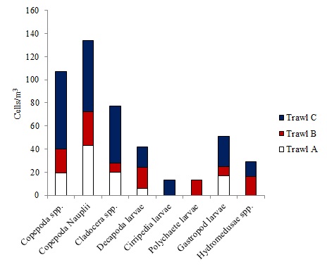
Figure 10.1 indicates that there was a higher abundance of zooplankton at Trawl C with 248 indivuals per m3 in total. This is followed by Trawl B at 113 individuals per m3and then Trawl A with 105 individuals per m3. The number of species present in trawl B was highest followed by C then A with 8, 7 and 5 species respectively.  Copepoda Nauplii were most abundant in all trawls followed by Copepoda spp. Species that were not present in trawl A that were present in trawls B and C were Polychaete larvae and Hydromedusae spp. Cirripedia larvae didn’t appear at all until trawl C.

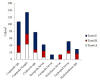
Figure 10.1: Zooplankton abundance in cells/m³ from the 3 trawls taken at Stations 2 (trawl A), 5 ( trawl B) and 7 (trawl C) 

PHYTOPLANKTON

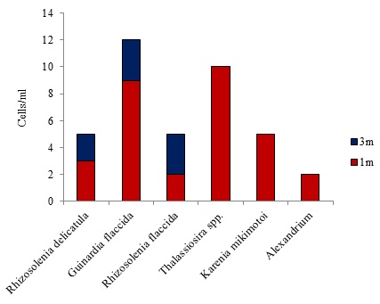
Phytoplankton abundance was highest at Station 2 (Figure 10.2), not only was there a higher diversity, there was also a higher number of cells per ml at a total of 39cells. Only R. delicatula, G. flaccida and R. flaccida were present at both 3m and 1m with G. flaccida being most abundant over the water column at 12cells/ml. Thalassiosira spp was most abundant at 1m at 10cells/ml.

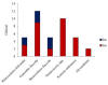
Figure 10.2: phytoplankton abundance in cells/ml of each recorded species taken at the sample depths of 3m and 1m

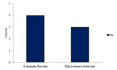
At station 4 (Figure 10.3), no cells were present in our sample at 3m, however, the number of G. striata exceeded the number of any cells found at all other depths and sites with 18cells/ml. Station 7 (Figure 10.4) exhibited the lowest number of cells and the lowest diversity with only G. flaccida and R. imbricate at 4 and 3 cells/ml respectively.

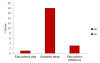
Figure 10.3: phytoplankton abundance in cells/ml of each recorded species taken at the sample depths of 3m and 1m

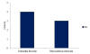
Figure 10.4: phytoplankton abundance in cells/ml of each recorded species taken at the sample depth of 9m

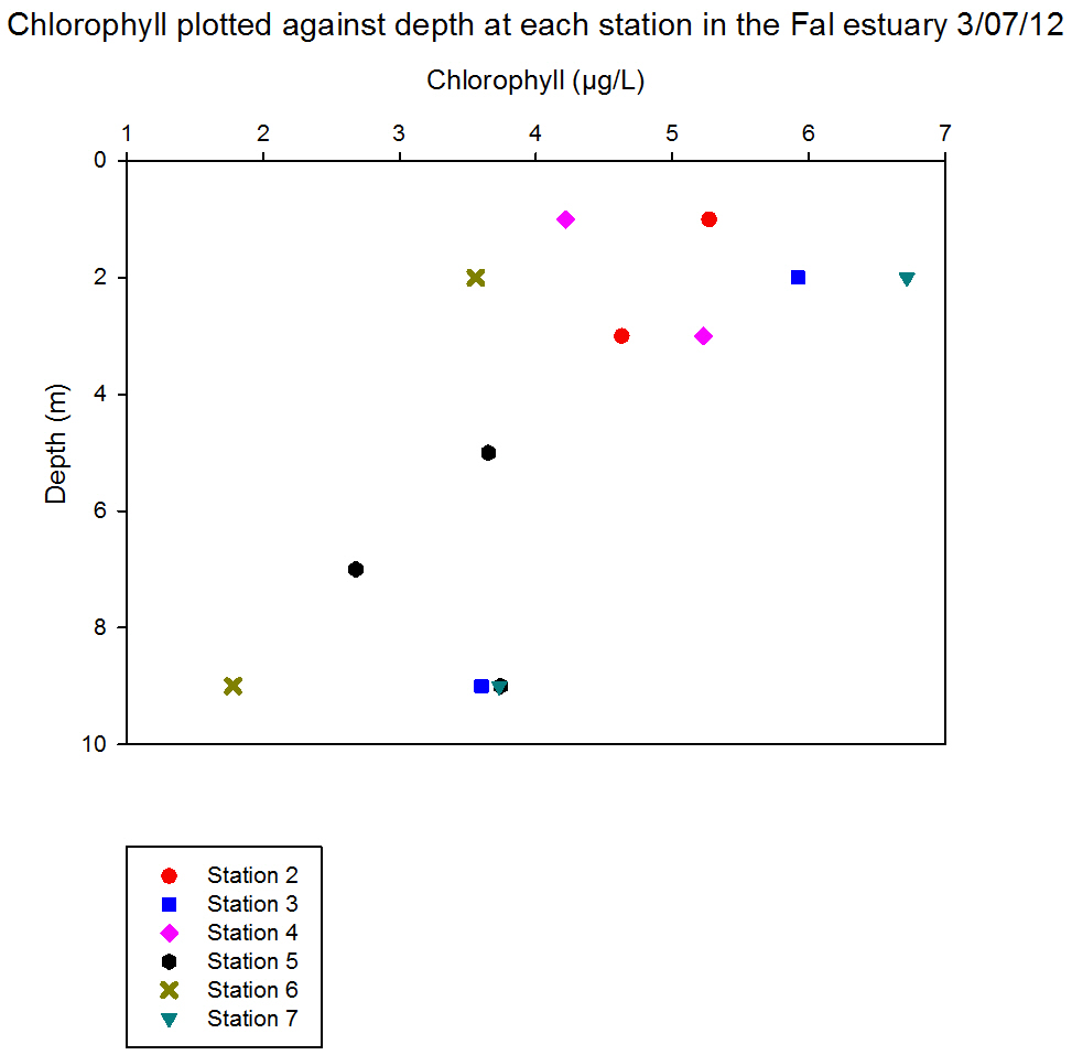
CHLOROPHYLL

Figure 10.5 indicated that the highest chlorophyll concentration recorded was at station 7 at the mouth of the estuary at 2m depth. The lowest was recorded at station 6 at 9m depth. At all stations sampled at, with the exception of station 3, the chlorophyll concentration recorded decreased with depth. At Station 3, the chlorophyll concentration recorded increased from 4.22 µg/l at 1m depth to 5.22 µg/l at 3m depth. There appeared to be no clear trend between chlorophyll concentrations and position along the estuary, more samples would need to be collected from a range of positions.

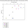
Figure 10.5: Chlorophyll plotted against depth from station 2 to station 5

PONTOON REPORT

INTRODUCTION 

Date: 05/07/2012

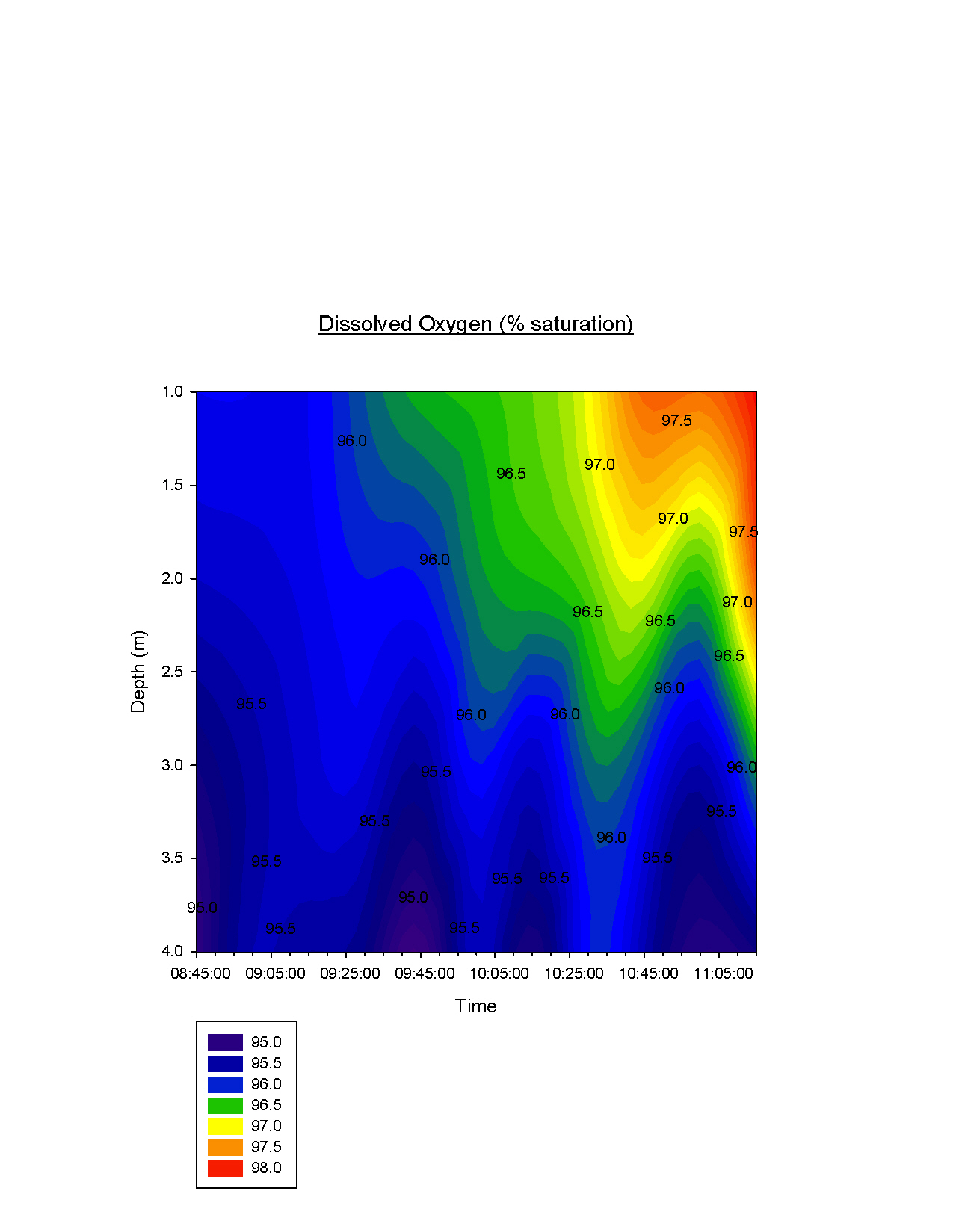
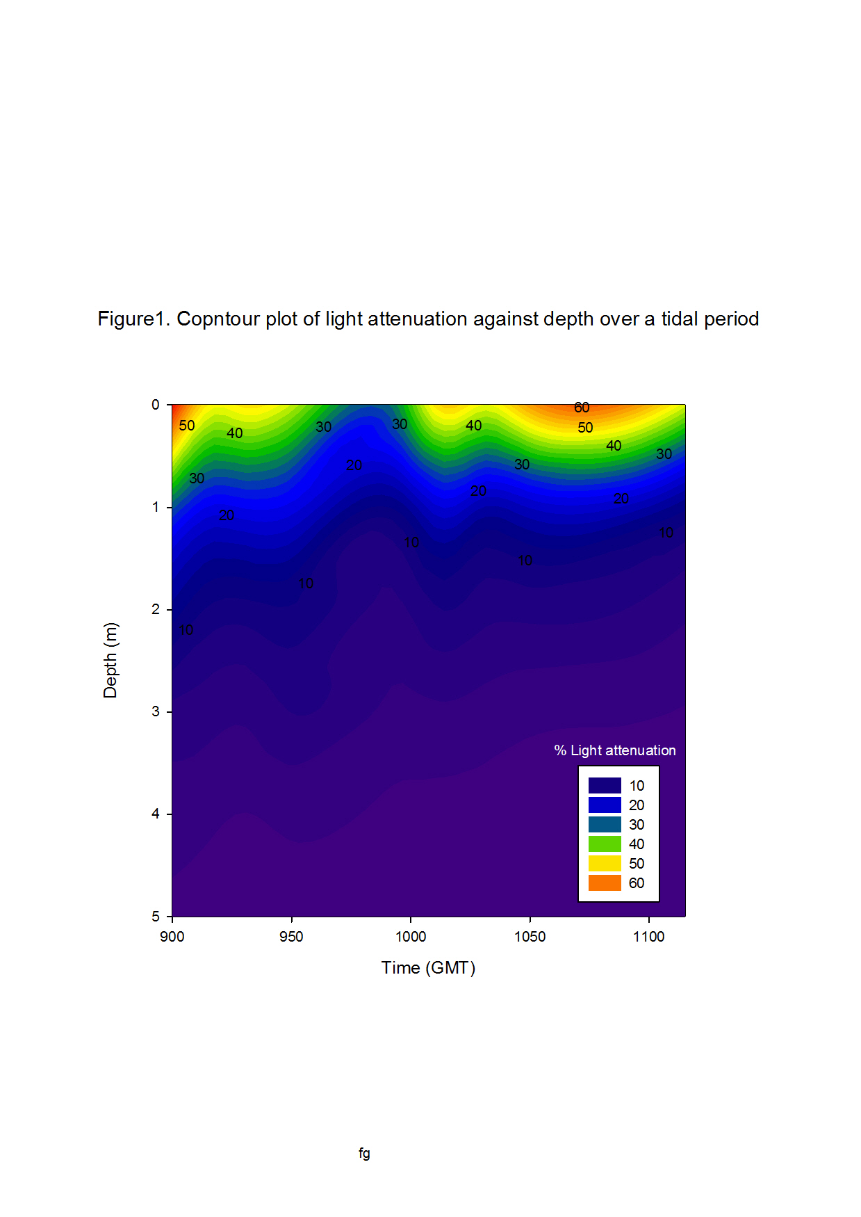
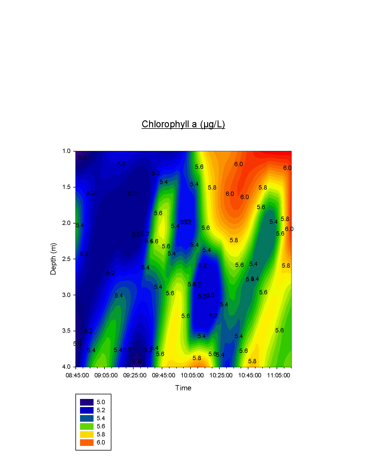
The aim of our research at the pontoon in the Fal estuary was to collect data for a time series within a fixed point of the Fal estuary during a tidal cycle. The equipment we used included a YSI multiprobe and a light sensor. A YSI multiprobe collects data on the temperature (°C), salinity, depth (m), acidity (pH), chlorophyll a (µg/L) and dissolved oxygen (% saturation). The light sensor detects irradiance levels in air and water in order to calculate light attenuation. We were unable to use to current meter due to technical difficulties.

METHODS

Measurements began at 0845 and were taken every 15 minutes until 1145 to give an idea of changes during the tidal cycle. Measurements were taken using a YSI multiprobe and a light sensor. The instruments were lowered into the water column at 1m intervals, until 4m depth and then recorded back up the water column as well. The data below has been plotted in contour plots to show the parameters in a 2D graphical manner.

YSI MULTIPROBE

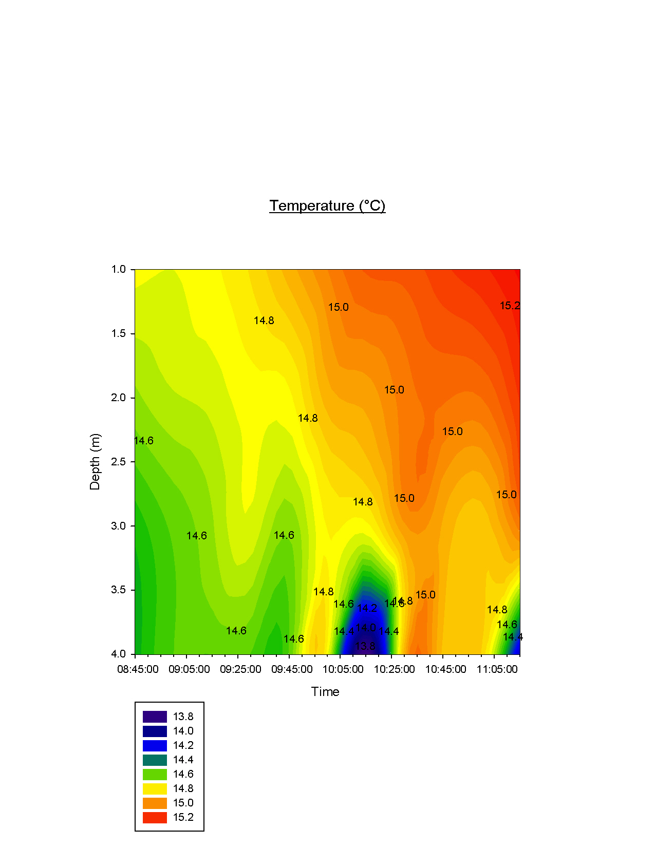
Figure 11.1. Temperature – Between 8:45-11:15 GMT it is clear that the surface waters get gradually warmer. When we first measured the temperature at 08:45 the surface waters were 14.6°C. By 11:15°C the water was 15.2°C. There is also a temperature gradient between the surface waters and the bottom waters, with the surface waters being much warmer. The temperature gradient intensified with time; at 08:45 the surface waters were 0.2°C warmer than the deeper waters, however by 11:45 the surface waters were 1.2°C warmer than the bottom waters.

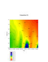
Figure 11.1: Temperature (⁰C)  plotted with depth showing changes over time from 08:45-11:15GMT.

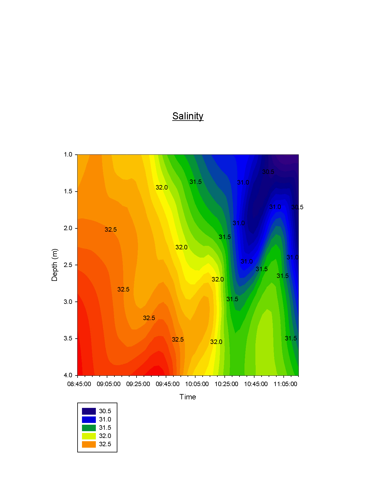
Figure 11.2. Salinity – The salinity at the fixed point in the estuary appeared to change in layers. At 08:45 the salinity was around 32.5 in the surface layers and was slightly higher in the bottom waters. By the end of the time series the salinity had decreased to 30.5 as the time approached low water (13:35). Throughout the series the deeper bodies of water remained more saline. This is because the more saline a body of water is, the greater it’s density. At the beginning of the time series the halocline was much more intense with a salinity difference of around 2.5 units whereas at 11:45 the difference is around 1.5 units.

Figure 11.2: Salinity plotted against depth showing changes over time from 08:45-11:15GMT.

Figure 11.3. – As the tidal cycle continued it appeared that the water column became more alkaline. At 08:45 the pH was 8.66 in the surface waters and by 11:45 it had risen to 8.70. This could also be because there was a period of rain at 10:15, diluting the water column and therefore increasing the pH. The pH was higher and therefore more alkaline in the surface layers of the water column. However, throughout the period of time we were sampling the pH only varied by 0.04. There was little difference between the pH of the surface waters and the bottom waters of the water column, usually only varying by 0.01pH.

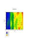
Figure 11.3: Acidity(pH) plotted against depth showing changes over time from 08:45-11:15 GMT

Figure 11.4 – At the beginning of the times series the levels of phytoplankton (chlorophyll a) were greater in the bottom levels of the water column. However as the day continued and the temperature and dissolved oxygen levels began to increase, the levels of chlorophyll a began to rise as well, especially in the surface layers. In the surface layers at 08:45 the levels of chlorophyll a were 5.0µg/L but by 11:15 they had increased to 6.0µg/L.  This could possibly be due to migratory patterns of the phytoplankton, for example diel migrations.

Figure 11.4: Chlorophyll a (µg/L) plotted against depth showing changes over time from 08:45-11:15GMT.

Figure 11.5 – The levels of dissolved oxygen increased throughout the time series. At 08:45 the levels of dissolved oxygen were around 95%, whereas they increased to 97.5% in the surface of the water by 11:15. At the beginning of the time series the levels of dissolved oxygen showed little variation throughout the vertical profile, remaining at 95% dissolved oxygen. However, by the end of the time series the levels of dissolved oxygen were greatest in the surface levels at 97.5% and lowest at the bottom of the water column, remaining at 95.0% dissolved oxygen. This is most likely due to changing of the tides aerating the water column and increased phytoplankton activity (refer to figure 4), photosynthesising and adding oxygen to the surrounding water.

Figure 11.5: Dissolved Oxygen (% saturation) plotted against depth showing changes over time from 08:45-11:15GMT.

Light Sensor

The contour plot (fig5) for light intensity shows a high percentage light attenuation at 50-60% in the surface depths above 1m. After 2m depth the percentage light attenuation decreased rapidly to less than 10% light attenuation. At 09:45 GMT there was a heavy rain shower, this is clearly visible at this time as % light attenuation at the surface is greatly reduced to less than 20%. This is due to increased turbidity of the surface water due to rain.

Figure 11.6 shows a decrease in percentage light attenuation as the ebbing tide progresses to low tide.  At 08:45 the percentage light attenuation was 62.6% at 0m and at 4m was 4.98%. By 11:15 the percentage light attenuation was 44.84% at 0m and 4.0% at 4m. When the water level decreased during ebbing tide the light sensor could only be deployed to 4m because the sea floor was reached. As the ebbing tides reached low water the velocity of the outgoing tides increase which may have increased turbidity of the water column as you move towards low tide. However, as the current meter was not working on the day this is not definitive.

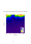Figure 11.6: A contour plot showing changes in light attenuation against depth over time from 08:45-11:15GMT

Back to top

GEOPHYSICS

OVERVIEW

The aim for the geophysics investigation was to generate a benthic habitat survey map with the use of sediment grabs, an ROV and side scan sonar. However, due to legal reasons, technical problems with the equipment and the relatively rough conditions, it was not possible to use this equipment. Instead we resorted to using a drop camera and inherited data to produce a habitat map of the Carrick Roads section of the Fal estuary.

Geophysics poster

Back to top