|
Falmouth, 2012 |

| Group 1 |
| INTRODUCTION |
| EQUIPMENT |
| OFFSHORE |
| GEOPHYSICS |
| ESTUARY |
| CONCLUSION |
| REFERENCES |
| Click on the links above to navigate the site |
| Veronica Madsen |
| Hanae Matsui |
| Chris McEntee |
| Cathryn Quick |
| Alice Trevail |
| Grace Verity |
| Eric Wade |
| Annie Allen |
| Colleen Bove |
| Melissa Brandner |
| Mat Cobain |
| Laura Dell |
| Chris Driver |
| Emmeline Gray |
| Danja Höhn |
|
Falmouth, 2012 |
| INTRODUCTION |
|
Although several conservation efforts have been taken, the long term input of heavy metals such as Sn, Cu, Pb, Fe, and Ag from mining activities, has polluted the area. The previous study of the Fal Estuary showed that some species in the estuary contain abnormally high concentrations of heavy metals (Bryan and Gibbs, 1983). The flooding of East Wheal Rose mine in 1846 and the now-closed Geevor Tin Mine in 1992 polluted the area severely. In recent years, industrial use of the port has increased pollution impacts due to the growing number of moored vessels, as well as discharge of pesticides from agricultural land. From the 25th of June to the 6th of July 2012, 15 marine biology and oceanography students from the University of Southampton investigated biological, chemical, and geophysical processes of the Fal Estuary and the surrounding waters. Studies of the estuary and coastal waters were carried out to collect data for analysis. The Falmouth field course is an applied learning opportunity for students to use the methods and skills obtained during the previous years. Throughout the course, the students aim to gain a better understanding of the overall impacts to the estuarine community and reach a consensus on how nature takes its course. This web page summarizes the boat work and lab results from Group1 during the Falmouth excursion. |


| EQUIPMENT | ||
| VESSELS | ||
|
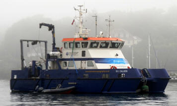
R.V. Callista |
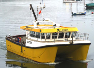
Xplorer |
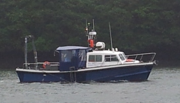 R.V. Bill Conway |
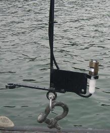
| IN-SITU INSTRUMENTS | ||
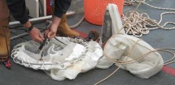 Plankton net |
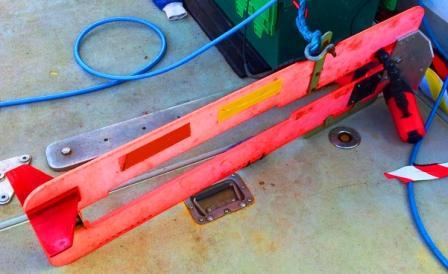
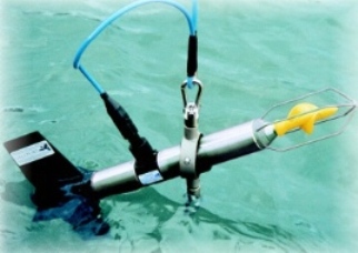
Sidescanner |
 Drop camera |
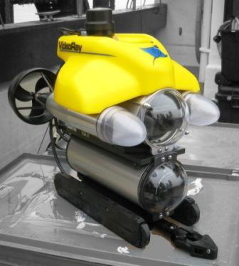 ROV REX (Remotely operated vehicle for Education and eXploration) Twitter: @rov_REX |
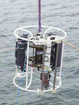 CTD frame with a rosette of Niskin bottles |
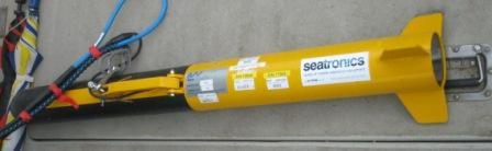
 ADCP (Acoustic Doppler Current Profiler) |
|
Irradiance meter |
Current meter |
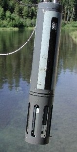 YSI probe |
| OFFSHORE | |||||||||||||||||||||||||||||||||||||||||||||||||||||||||||||||||||||||
| INTRODUCTION | |||||||||||||||||||||||||||||||||||||||||||||||||||||||||||||||||||||||
|
In the coastal shelf sea of the Western English Channel, light and nutrients vary with depth and time of year (Al-Moosawi et al., 2009). Offshore of Falmouth during the summer months deep thermal stratification can be seen, due to an increase in irradiance levels as the incidence angle of the sun increases (Pidwirny, 2006) and a decrease in tidal mixing. The extent of the stratification is determined by water depth and tidal strength. Closer to the estuary the water column stratification may be determined by density structure of the water column, by input of freshwater and wind strength. A coastal front forms in the water column where well mixed cooler water meets thermally stratified water from offshore (Pingree et al., 1978). It is a region of larger than average horizontal gradient. The vertical mixing of the water column has an effect on the physical, chemical and biological properties of the surface layer of the ocean. Phytoplankton populations may be altered by factors affecting their growth (light and nutrients) and mortality (predation by zooplankton), whereas zooplankton species will be affected by food (phytoplankton) and predation. Dissolved oxygen distribution is an indicator of the balance between autotrophy and heterotrophy. Summer stratification leads to the depletion of surface nutrients and nutrient-rich deep waters, therefore the rate of upward mixing of nitrate, phosphate and silicate is important for phytoplankton species. The transition zone between two zones at the front also provides optimal conditions for phytoplankton growth. Our aim is to collect data and evaluate it in order to determine the direct and indirect effects of vertical mixing processes, in the waters off Falmouth, on the chemical and physical structure of the water column and structural and functional properties of plankton communities. On the 25th June 2012 at 0930 GMT, the offshore survey was undertaken. Data were collected at 4 stations along a transect with a bearing of 160°. High tide for the day of the survey was at 0835GMT with a height of 4.6m and low tide was at 1504GMT with a height of 1.1m. The details of the 4 stations can be seen in table 1. Samples were collected at stations 1, 3 and 4; station 2 was used as a reference to determine the water structure and the position of the coastal front relative to the vessel, however no samples were collected. Due to spring tides on the day of the survey, the coastal front was further offshore than expected because of stronger tidal mixing, and station 2 was a necessary reference. An ADCP profile was taken throughout the survey and used to determine the locations of the stations, dependent on water column structure analysis from backscatter profiles. The depths of samples were determined from a CTD profile at each station. The instruments used within this survey were: Vertical plankton net, CTD with a rosette of Niskin bottles, ADCP, Secchi disk. |
|||||||||||||||||||||||||||||||||||||||||||||||||||||||||||||||||||||||
| CTD PROFILES | |||||||||||||||||||||||||||||||||||||||||||||||||||||||||||||||||||||||
|
Station 1 was the furthest inshore station that was sampled; this meant it was the shallowest, down to around 35m. The CTD cast (Figure 1.1) shows a relatively well mixed water column with a slight increase in salinity and decrease in temperature with depth. The thermocline is at around 12m. At the surface the water temperature is 13.1°C. In the first 5m this drops to 12.6°C. By 12m depth the temperature has dropped to 12.4°C. It then stays constant down to 31m. At the surface the chlorophyll concentration is 0.08mg/m3. Between the surface and 10m depth it increases to 0.14 mg/m3. The highest level of chlorophyll is above the thermocline. By 32m depth it has decreased to 0.16mg/m3. The chlorophyll values fluctuate a lot but only within 0.02mg/m3. The 1% light level is at 22.42m. The least saline water is at the surface because it is less dense, although the changes in salinity are less than 0.5 in total. At the surface the salinity is 34.95. In the first 5m it increases to 35.22. Between 5m and 12m it increases to 35.25. It then stays constant down to 32m when is drops to 35.22 again. Station 3 was further out than station 1 which allowed a deeper CTD cast (Figure 1.2) to be taken, down to around 65m. The temperature dropped fairly steadily but there is a thermocline at around 15m after which the temperature continues to decrease but less rapidly. At the surface the water temperature is 13.0°C. In the first 10m this drops to 12.5°C. It then decreases fairly constantly until it reaches 12.25 at around 65m depth. There is a chlorophyll maximum at station 3. At the surface the chlorophyll concentration is 0.12mg/m3. It increases to 0.18 mg/m3 by 7m depth. It then decreases fairly constantly down to 20m depth where it is 0.10 mg/m3. The chlorophyll value fluctuates a lot but within 0.02 mg/m3. The bottom of the chlorophyll maximum coincides with the thermocline at 15m. This is above the 1% light level, which is at 26.74m. The salinity is lower at the surface than at depth because less dense river water floats on denser sea water. This is shown by the changes in salinity shown on the depth profile even though the changes are very small. At the surface the salinity is 35.36. In the first 10m it increases to 35.40. It then increases fairly constantly down to 30m when it is 35.41 before decreasing fairly constantly until it reaches 35.40 at around 65m depth. Station 4 was the furthest offshore station and allowed the deepest CTD cast (Figure 1.3)to be taken, down to around 75m. The temperature dropped in steps until the thermocline at 20m depth. At the surface the temperature is 13.2°C. It then decreases rapidly to 12.8°C at 5m depth. It then stays fairly constant down to 20m depth when it decreases rapidly to 12.5°C. It then continues to drop gradually until it reaches 12.4°C at 70m depth. There is a clear subsurface chlorophyll maximum at station 4. At the surface the chlorophyll is 0.11mg/m3. It then increases rapidly to 0.20 mg/m3 by 5m depth. It then stays constant down to 20m before decreasing rapidly to 0.09 mg/m3 by 25m. This is the bottom of the chlorophyll maximum. The bottom of the chlorophyll maximum coincides with the main thermocline and the 1% light level. The 1% light level is at 26.45m. A secchi disk was used at station 4 which gave an SD depth of 9m; from this the 1% light level is calculated as 27m. The salinity is lower at the surface because less dense river water will sit on top of more dense sea water. This is shown by the lower salinity water at the surface and the higher salinity water below 5m depth even though the salinity change is minute. At the surface the salinity is 34.35. It increases to 35.40 by 5m depth. It then increases gradually to 35.41 by 70m depth.
Comparison of all three stations: Irradiance decreases exponentially with depth. Each of the three stations was warmer at the surface than at depth. Each of the stations was more saline at depth than at the surface. In the top 5m of each station there is less saline water. Below this it is fairly uniform. The greatest change in salinity was at station 4 which had an increase of 1.06 between the surface and bottom values. There are subsurface chlorophyll maxima above the 1% light level at all the stations; the bottoms of these chlorophyll maxima coincide with the thermoclines. Station 4’s is the most pronounced, then station 3’s, then station 1’s.
|
Figure 1.1. Depth profiles from the CTD for station 1. Arrows on the depth axis show the depths, at which Niskin samples were taken. Horizontal dashed line shows the depth of 1% of surface light irradiance. |
||||||||||||||||||||||||||||||||||||||||||||||||||||||||||||||||||||||
|
Figure 1.2. Depth profiles from the CTD for station 3. Arrows on the depth axis show the depths, at which Niskin samples were taken. Horizontal dashed line shows the depth of 1% of surface light irradiance. |
|||||||||||||||||||||||||||||||||||||||||||||||||||||||||||||||||||||||
|
Figure 1.3. Depth profiles from the CTD for station 4. Arrows on the depth axis show the depths, at which Niskin samples were taken. Horizontal dashed line shows the depth of 1% of surface light irradiance. |
|||||||||||||||||||||||||||||||||||||||||||||||||||||||||||||||||||||||
| ADCP PROFILES | |||||||||||||||||||||||||||||||||||||||||||||||||||||||||||||||||||||||
|
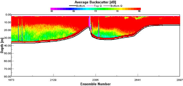
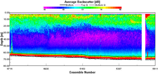
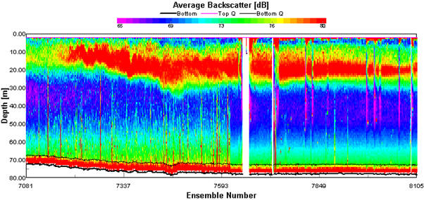
Backscatter plots from the ADCP can be used to analyse biological factors in the water column. High backscatter can be seen where there are areas of high particulate matter in the water column which could be due to a high abundance of plankton (Flagg & Smith, 1989). Phytoplankton can be found in high abundance at water mass boundaries and along thermoclines. During the survey, the in-situ backscatter profiles were monitored to determine changes in water structure, the location of a frontal system and thermal stratification. The ADCP was run for the duration of the survey. Transect 1 backscatter plot (Figure 1.4) shows the transect from Falmouth harbour to the coastal waters around Blackrock. The waters were shallow, reaching a max depth of 32.68m at station 1. Estuarine inputs result in higher nutrient inputs in this area and high backscatter of 80dB can be seen throughout the water column in the shallowest waters at the start of the transect. The high backscatter could be because of increased suspension of particulate matter from the seabed and abundance of plankton. As depth increases along the transect there is a stratification between high backscatter at the surface down to 18m then lower backscatter below this depth of 74dB. At around the same depth as the decrease in backscatter, the light levels become too low for photosynthesis to occur. The water column in this area is well mixed, therefore light is likely to be the determining factor in phytoplankton distribution, and subsequently zooplankton distribution as a result of grazing control, hence why backscatter is higher at the surface. Transect 2 (Figure 1.5) shows the water column from station 1 to station 2. There was high backscatter of 80dB at the surface during this transect, but low backscatter throughout most of the plot, which correlates with a well-mixed water column. The ADCP plot between station 2 and 3 (Figure 1.6) shows a well-mixed water column, which is consistent along the 897m transect. High backscatter at the surface of 76dB to 80dB signifies high plankton abundance. High plankton abundance at the surface is due to the limiting factor for growth being light and the highest light levels being at the surface. The amount of backscatter at the surface has decreased from the previous transect. This may be because of a decrease in nutrients as depth and distance from the coast increases. The ADCP profile from stations 3 to 4 (Figure 1.7) shows the development of a frontal system and thermal stratification in the water column. High backscatter is a proxy for plankton. The change in backscatter from the surface to 20m depth is from 69dB to 80dB, showing an increase in particles in the water column. The transect shows the passing of a front as backscatter increases though out the water column at 150m along the transect into offshore waters with stratification which is seen at the end of the transect. At the end of the transect which correlates with our station 4 there is high backscatter between 15m and 20m, which could indicate a thermocline if the increased backscatter is because of increased plankton. This can be confirmed by other forms of data collected. At frontal systems, nutrients are brought to the surface by upwelling, resulting in an increase in phytoplankton abundance. |
Figure 1.4. ADCP plot showing the average backscatter throughout the water column along the ships path from Falmouth Harbour to Blackrock (50˚08.738 N, 005 ˚01.4721 W). |
||||||||||||||||||||||||||||||||||||||||||||||||||||||||||||||||||||||
|
Figure 1.5. ADCP plot showing the average backscatter throughout the water column along the ships path from Station 1: Blackrock (50˚ 08.738 N, 005 ˚01.4721 W) to Station 2 (50˚ 03.133 N, 004 ˚ 58.587 W). |
|||||||||||||||||||||||||||||||||||||||||||||||||||||||||||||||||||||||
|
Figure 1.6. ADCP plot showing the average backscatter throughout the water column along the ships path from Station 2 (50˚ 03.133 N, 004˚ 58.587 W) to Station 3 (50˚ 00.406 N, 004˚ 57.766 W). |
|||||||||||||||||||||||||||||||||||||||||||||||||||||||||||||||||||||||
|
Figure 1.7. ADCP plot showing the average backscatter throughout the water column along the ships path from Station 3 (50˚ 00.406 N, 004˚ 57.766 W) to Station 4 (49˚ 56.142 N, 004˚ 56.922 W). |
|||||||||||||||||||||||||||||||||||||||||||||||||||||||||||||||||||||||
| RICHARDSON NUMBER | |||||||||||||||||||||||||||||||||||||||||||||||||||||||||||||||||||||||
|
The Richardson number (Ri) is a dimensionless number, which, when applied to oceanography, can be used to compare the stabilisation of the water column as a result of buoyancy with the destabilisation from shear current flow. From looking at the depths of laminar or turbulent flow within the water column, it can give an indication of stratification. Richardson number can be calculated as follows:
Ri =
Where: g = gravity (9.81m/s2) ρ = density (kg/m3) from CTD profiles u = velocity (m/s) from ADCP profiles If the calculated Richardson number is less than 0.25, then it can be assumed that horizontal shear is significant enough to overcome stratification, and mixing can occur. If Ri is calculated to be above 1, horizontal shear is not significant, and vertical stratification can develop. If Ri falls between 0.25 and 1, then it is considered to be in an intermediate state, either stratification or mixing may be developing. For all stations, most Richardson numbers calculated were less than 0.25 (Figure 1.8, Figure 1.9, Figure 1.10), therefore the majority of the water column can be assumed to be well mixed. Stations 1 and 3 showed stable flow at some depths, however only over a range too small to allow stratification, as can be confirmed by the CTD profiles, which showed only a small amount of difference between temperature and salinity over the entire water column (Figures 1.8 - 1.10). There is less correlation between the sets of data at station 4 however. The CTD profile indicated a higher degree of stratification (Figure 1.10), however all values of Richardson number calculated were less than 1. Any miscorrelation in data may be due to the location of the velocity values from the ADCP not correlating exactly with the location of the density values of the CTD. This is because the boat may have drifted between the time the ADCP was turned off at each station and the time the CTD profile was taken.
|
Figure 1.8. Richardson numbers calculated for the offshore station 1 |
||||||||||||||||||||||||||||||||||||||||||||||||||||||||||||||||||||||
|
Figure 1.9. Richardson numbers calculated for the offshore station 3 |
|||||||||||||||||||||||||||||||||||||||||||||||||||||||||||||||||||||||
|
Figure 1.10. Richardson numbers calculated for the offshore station 4 |
|||||||||||||||||||||||||||||||||||||||||||||||||||||||||||||||||||||||
| CHEMISTRY | |||||||||||||||||||||||||||||||||||||||||||||||||||||||||||||||||||||||
|
Niskin bottles attached to the CTD Rosette were fired at depths throughout the water column at each of the three stations measured. Depths were not selected at random, but were selected based on findings of the CTD downcast, so as to achieve the most useful and interesting results. Samples were collected both at depth and at the surface of the water column, and also a sample at the peak of and just below the halocline or thermocline, whichever was most prevalent. For Station 1, only three samples were collected because the water column was relatively well mixed (Figure 1.11, Figure 1.12, Figure 1.13). All nitrate values were too low for detection, hence exclusion of any results. At station 1 (Figure 1.11), both nutrients (silicate and phosphate) were present in a higher concentration at depth than at the surface. Silicate presented a constant increase from 0.875mmol/l at 1.106m depth to 1.424mmol/l at 32.68m depth. Phosphate presented a slight subsurface maximum. It increased from 0.123mmol/l at 1.106m depth to 0.242mmol/l at 8.251m depth, and then decreased again to 0.236mmol/l at 32.68m depth. Dissolved oxygen increased from 49.8% saturation at 1.106m depth to 95.3% saturation at 32.68m depth. Chlorophyll was lower at depth (0.77mg/m3) than at the surface (1.44mg/m3) however presented a sub-surface maximum (1.74mg/m3) at the bottom of the well-mixed layer (8.251m). At station 3 (Figure 1.12), both nutrients (silicate and phosphate) were present in a higher concentration at depth than at the surface. Silicate presented an increase from 0.678mmol/l at 1.021m depth to 1.597mmol/l at 64.4m depth. Phosphate increased from 0.130mmol/l at 1.021m depth to 0.260mmol/l at 64.4m depth. Despite an overall increase in concentration with depth, both nutrients were lowest at 5.951m depth (silicate concentration: 0.590mmol/l, phosphate concentration: 0.106mmol/l). Dissolved oxygen increased overall with depth from 89.37% saturation at 1.021m, to 116.6% saturation at 64.4m, however also was lowest at 5.95m (84.6%). Chlorophyll was lower at depth (0.78mg/m3) than at the surface (2.45mg/m3) however presented a sub-surface maximum (2.51mg/m3), which corresponds with the sub-surface minima of nutrients and dissolved oxygen. At station 4 (Figure 1.13), both nutrients (silicate and phosphate) were present in a higher concentration at depth than at the surface. Silicate presented an increase from 0.514mmol/l at 1.083m depth to 1.400mmol/l at 68.47m depth. Phosphate increased from 0.177mmol/l at 1.083m depth to 0.283mmol/l at 68.47m depth. There was no surface measurement of dissolved oxygen at station 4, however it increased from 97.7% saturation at 11.04m depth to 122.8% saturation at 68.47m depth. Chlorophyll was lower at depth (0.610mg/m3) than at the surface (5.616mg/m3). Discussion Concentration of all nutrients measured were very low, which agrees with the findings of other studies in the western English Channel in June, compared to other times of year (Butler, Knox & Liddicoat, 1979). The hydrodynamics of the coastal region off Falmouth favour considerable spring phytoplankton blooms, in particular of diatoms, which are very efficient at utilising the nutrients available. As a result of this nutrients are significantly depleted in the summer months. Nitrate levels were too low to measure, indicating that nitrogen is the limiting nutrient for phytoplankton growth in the coastal region around Falmouth (Armstrong, Butler & Boalch, 1970). At stations 1 and 3 (Figures 1.11 and 1.12, respectively) chlorophyll exhibits a sub-surface maximum. This is often found as a result of photo-inhibition at the highest light levels at the surface, and possibly as a response to lower light levels deeper in the water column. For all stations, chlorophyll was significantly higher at the surface than at the deepest point, showing that a higher biomass of photosynthesising organisms are located at the surface, as a pose to at depth, corresponding with the higher light levels at the surface to facilitate this (Sathyendranath and Platt, 2008). Although no sub-surface maximum was found at station 4 (Figure 1.13), surface chlorophyll levels were significantly higher than at the other two stations. This may be related to the position of station four on the oceanic side of the front, within thermally stratified waters. At station two, high levels of chlorophyll in the peak of the halocline (i.e. at the point of most change) correspond with lowest nutrient levels and the lowest saturation of dissolved oxygen. This indicates that highest biomass of both phytoplankton and zooplankton is located at the base of the upper mixed layer. At depth at all stations, lower chlorophyll levels correspond with higher nutrient levels and less that 1% of surface light levels. |
Vertical depth profiles of the nutrient concentrations (phosphate and silicate), chlorophyll concentrations and dissolved oxygen saturation at station 1 (Black rock: 50° 08.738 N, 005° 01.4721 W). Samples were collected at 10:30 GMT (HW+2). |
||||||||||||||||||||||||||||||||||||||||||||||||||||||||||||||||||||||
|
Figure 1.12. Vertical depth profiles of the nutrient concentrations (phosphate and silicate), chlorophyll concentrations and dissolved oxygen saturation at station 3 (50° 03.133 N, 004° 58.587 W). Samples were collected at 12:15 GMT (HW+4). |
|||||||||||||||||||||||||||||||||||||||||||||||||||||||||||||||||||||||
|
Vertical depth profiles of the nutrient concentrations (phosphate and silicate), chlorophyll concentrations and dissolved oxygen saturation at station 3 (50° 00.406 N, 004° 57.766 W). Samples were collected at 13:10 GMT (HW+5). |
|||||||||||||||||||||||||||||||||||||||||||||||||||||||||||||||||||||||
| BIOLOGY | |||||||||||||||||||||||||||||||||||||||||||||||||||||||||||||||||||||||
|
Phytoplankton samples were taken at 3 stations using Niskin bottles attached to a CTD: 3 samples at Station 1 (Blackrock Latitude: 50˚08.738 N Longitude: 005 ˚01.4721 W) (Table1), 4 samples at Station 3 (Latitude 50 ˚00.406N Longitude 004 ˚57.766W) (Table 2) and 4 samples at Station 4 (Latitude 49 ˚56.142N Longitiude 004 ˚56.922W) (Table 3.) 100ml of each water sample was transferred to a glass bottle containing an iodine solution and later analyzed under a microscope by counting individual cells. Chlorophyll samples and replicates filtered from seawater were taken at each station as well and stored in an acetone solution until analysis. Zooplankton samples were taken at the 3 stations using a net with a 50cm diameter and a 200μm mesh filter size and preserved with formalin until analysis. The individual cells were counted from 10ml samples and converted to total per m3. The highest concentration of phytoplankton was found at Station 1 (388 total), followed by Station 3 (265 total) and then Station 4 (168 total). The five most common species were Rhizosolenia setigera (64 total), Chaetoceros sp. (76 total), Rhizosolenia delicatula (106 total), Leptocylindius danicus (163 total), and Guinardia flaccida (166 total.) With the exception of Rhizosolenia setigera, which was mainly found at Station 1, all of these species were not only found in high numbers, but throughout most of the samples at all of the stations. Overall, around 92% of the phytoplankton found at the three stations were diatoms. This suggests a mixed vertical distribution though most of the samples (Holligan et al., 1984).
Table 1. Comparing the data from phytoplankton counts and chlorophyll levels against depth from Station 1.
Table 2. Comparing the data from phytoplankton counts and chlorophyll levels against depth from Station 3.
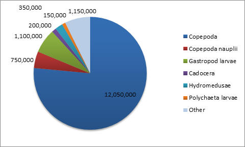
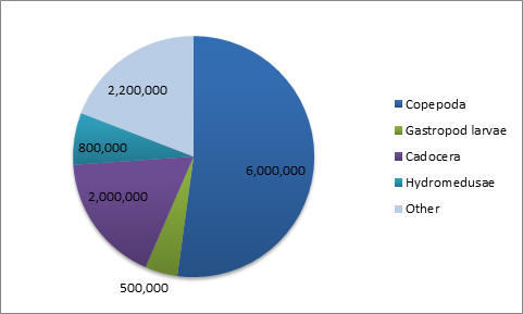
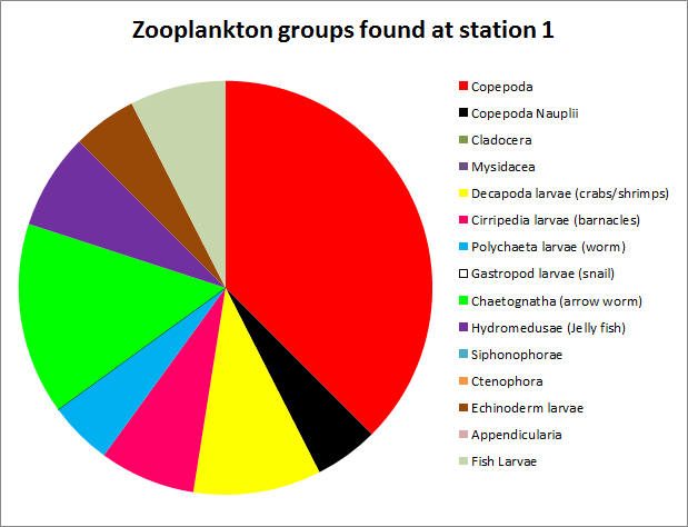
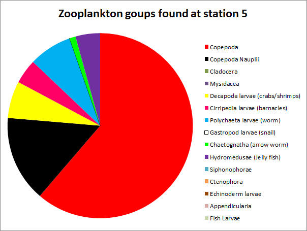
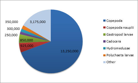
Table 3. Comparing the data from Phytoplankton counts and chlorophyll levels against depth from Station 4. The tables above compare phytoplankton counts and chlorophyll levels against depth. At Stations 1 and 3, phytoplankton were found in high numbers at the surface (samples 3 and 4 respectively). The surface sample at Station 4 had very low phytoplankton numbers, contradicting the very high chlorophyll concentration from the physical water sample. There were two samples taken in the middle of the thermocline (Station 3–Sample 3 and Station 4–Sample 3). The Station 3 thermocline sample did not have a high phytoplankton count, but this did contradict the chlorophyll levels in both the physical water samples and the CTD scan. The Station 4 thermocline sample had a very high total phytoplankton count and high chlorophyll levels for both the physical water samples and the CTD scan. Samples taken at the bottom of the thermocline were significantly higher in phytoplankton concentrations at Station 1 (Sample 2), and relatively high at Station 3 (Sample 2). They were very low at Station 4 (Sample 2). The deeper samples were less consistent over the three stations. At Station 1 (where the deepest depth was half as deep as the other two stations) the phytoplankton concentration was high, contradicting the chlorophyll levels in the physical water samples, but corresponding with the CTD chlorophyll levels. At Station 3, the phytoplankton count of Sample 3 (5.95m) appears to be anomalously low and, if excluded, the samples would correlate better with the two chlorophyll measurements. The phytoplankton concentrations at 68.47m of Station 4 were extremely low, which contradicts the chlorophyll levels in the physical water samples, but correlates with the CTD chlorophyll levels. In Figure 1.14, the manual phytoplankton counts from all samples at Station 1 were compared to the temperature and irradiance levels found using the CTD scanner. The phytoplankton and temperature follow a similar pattern. Phytoplankton increases around the thermocline and drops around the same depth as temperature does. Phytoplankton and irradiance also follow a similar pattern. As irradiance starts to fall, phytoplankton totals begin to drop. In Figure 1.15, the manual phytoplankton counts from all samples at Station 3 were compared to the temperature and irradiance levels found using the CTD scanner. The drop in phytoplankton clearly coincides with the drop in temperature, but there is also a strong, unexpected drop in phytoplankton in the middle of the thermocline. This was not found at any of the other stations. The phytoplankton and irradiance levels follow the same pattern as from Station 1, with the exception, again, of the drop in phytoplankton around 10m. In Figure 1.16, the manual phytoplankton counts from all samples at Station 4 were compared to the temperature and irradiance levels found using the CTD scanner. In Figure 5, temperature and phytoplankton coincide very well. There is a rise in phytoplankton around the thermocline, as was seen at Station 1 and the levels drop just as the temperature does. In Figure 6, the phytoplankton total follows the drop in irradiance quite closely and almost disappears entirely when irradiance nears zero. Zooplankton numbers (Figures 1.17 – 1.20) followed the pattern seen in phytoplankton. The highest concentration of zooplankton was found at Station 1 (19,100,000 total), followed by Station 3 (15,800,000 total) and Station 4 (3,800,000 total). By far the most widely found group of zooplankton was Copepoda (36,300,000 total), which could be due to the large number of diatoms present in our samples, which are a prominent group in the copepod diet (Kleppel, 1993). (Other includes: Decapoda larvae, Cirripedia larvae, Chaetognatha, Siphonophorae, Echinoderm larvae, Appendicularia, Fish larvae, Phoronida, Bryozoae)
|
CLICK TO ENLARGE Figure 1.14. Phytoplankton numbers against temperature, irradiance and depth at Station 1 |
||||||||||||||||||||||||||||||||||||||||||||||||||||||||||||||||||||||
|
Figure 1.15. Phytoplankton numbers against temperature, irradiance and depth at Station 3 |
|||||||||||||||||||||||||||||||||||||||||||||||||||||||||||||||||||||||
|
Figure 1.16. Phytoplankton numbers against temperature, irradiance and depth at Station 4 |
|||||||||||||||||||||||||||||||||||||||||||||||||||||||||||||||||||||||
|
CLICK TO ENLARGE Figure 1.17. Zooplankton species at station 1 |
|||||||||||||||||||||||||||||||||||||||||||||||||||||||||||||||||||||||
 CLICK TO ENLARGE Figure 1.17. Zooplankton species at station 3 |
|||||||||||||||||||||||||||||||||||||||||||||||||||||||||||||||||||||||
 CLICK TO ENLARGE Figure 1.17. Zooplankton species at station 4A |
|||||||||||||||||||||||||||||||||||||||||||||||||||||||||||||||||||||||
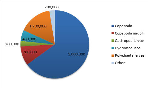 CLICK TO ENLARGE Figure 1.17. Zooplankton species at station 4B |
|||||||||||||||||||||||||||||||||||||||||||||||||||||||||||||||||||||||
| CONCLUSION | |||||||||||||||||||||||||||||||||||||||||||||||||||||||||||||||||||||||
|
From all of the data collected and analysed during this survey the results show that vertical mixing processes can influence the structure and functional properties of plankton communities. As the distance from the shore increased there was a visible change in water column structure, which reflects a change in vertical mixing processes. At the estuary mouth the shallow waters were tidally well mixed. The surface nutrients were highest at this location due to the influence of riverine input. The higher abundance of phytoplankton counted and the higher concentrations of chlorophyll recorded at the surface reflects the well-mixed water column structure. The ADCP data showed that plankton concentrations were high throughout the water column to roughly 20m deep, which roughly corresponds with the depth of the 1% light level. The vertical gradients in nutrient and chlorophyll concentration and dissolved oxygen saturation were more prominent than the horizontal gradients away from the shore. At all stations, chlorophyll concentration was restricted to above the 1% light level, which leads to the conclusion that vertical light attenuation is a key determining factor in phytoplankton distribution, in particular at station 1 where gradients of physical factors were slight. With distance from the shore, the thermocline had a higher degree of influence on phytoplankton distribution, and these parameters were closely linked. Zooplankton distribution follows phytoplankton distribution showing that the main control or limitation is food supply. Although no vertical profile or samples were taken, there was a clear front observed on the ADCP profile. There was a significant increase in backscatter over a large portion of the water column, likely to be caused by plankton and facilitated by upwelling of nutrients. Station 4 was located past the front. Stratified conditions were expected, however not observed. This may be as a result of the bad weather preceding the sample date; therefore temperatures were not sufficient for strong thermal stratification to occur. More prominent thermal stratification may be found in deeper waters offshore. |
|||||||||||||||||||||||||||||||||||||||||||||||||||||||||||||||||||||||
| GEOPHYSICS | |||||||||||||||||||||||||||||||||||||||||||||||||||||||||||
| AIM | |||||||||||||||||||||||||||||||||||||||||||||||||||||||||||
|
The aim of the geophysical survey in the Fal Estuary is to create a benthic habitat map of a small section. The Saint Mawes Harbour is currently being considered as a dredging location and therefore being the point of our data collection. Therefore, we are mapping the benthic habitat to determine the loss and risks associated with the potential habitat destruction. |
|||||||||||||||||||||||||||||||||||||||||||||||||||||||||||
| INTRODUCTION | |||||||||||||||||||||||||||||||||||||||||||||||||||||||||||
|
Marine habitat mapping is a fairly new industry that has taken off over the past decade. In creating a map of the seafloor physical distributions of habitats can be interpreted. Benefits of benthic mapping include: i. Supporting sustainable use of seabed resources ii. An eco-system based appeal to manage human activities iii. Monitoring the geographic context on a global scale iv. Identification and protection of Marine Protected Areas (MAPs) v. Understanding of marine ecosystems and processes, such as hydrography, water columns, species communities and climate. Only small sections can be sampled, but when several techniques are combined- habitat boundaries begin to appear. In the Saint Mawes Harbour, data was collected twice along three transects, once in the morning and again in the afternoon:
|
|||||||||||||||||||||||||||||||||||||||||||||||||||||||||||
|
Group 1 - AM Date: 28/06/2012 Location: Saint Mawes Harbour, Fal Estuary, Cornwall [50°03.04 N, 005°01.447 W] Sea state: calm in the morning getting more rough in the afternoon Wind: light breeze Cloud cover: 8/8 okta Vessel: MV Explorer Tide: Between neap and spring (moving toward neap). Low water: 05.29 GMT, 1.3 m Hight water: 11.26 GMT, 4.4 m Range: 3.1 m
|
Group 1 - PM Date: 28/06/2012 Location: Saint Mawes Harbour, Fal Estuary, Cornwall [50°03.04 N, 005°01.447 W] Sea state: Rough water with sea state 4 moving to 5 later in the day. Wind: moderate breeze Cloud cover: 5/8 okta with occasional sunshine Vessel: MV Explorer Tide: Ebbing tide, neap tides Low water: 06.29 BST, 18.15 BST, 1.3 m High water: 12.26 BST, 4.4 m Range: 3.1 m
|
||||||||||||||||||||||||||||||||||||||||||||||||||||||||||
The instruments used within this survey were: |
|||||||||||||||||||||||||||||||||||||||||||||||||||||||||||
| METHOD | |||||||||||||||||||||||||||||||||||||||||||||||||||||||||||
|
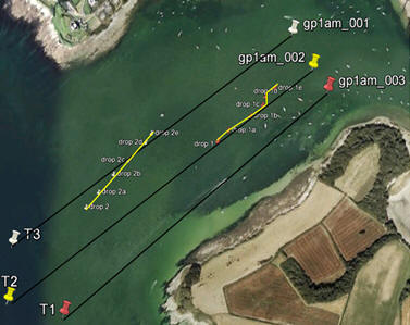
Video Analysis The video analysis of the bottom habitat was carried out by a Remotely Operated Vehicle (ROV) on Thursday June 28th, 2012. When the location was found, it was attached to a line and deployed into the water. The video was being monitored on board and recorded for further observations. In the lab, the video was observed to identify different features on the sea floor. Side Scan A tow fish was attached to the vessel to provide a subsurface dual frequency side scan sonar of the marine environment at frequencies of 114 kHz (am) and 410 kHz (pm). The signals are directly digitised in the tow fish and transmitted via a digital connection over a coaxial cable. The side scan was carried out along three parallel transect lines, with 100m spacing (Figure 2.1, right). The conditions in the morning were not optimal for the side scanner, however in the afternoon the conditions favoured sonar conduction. The frequency emitted from the sonar was either absorbed or reflected back to the transmitter. The signals obtained from the side scan were relayed back on board to the side scan sonar and quantified. The quantified data was displayed on a black and white scale, with the darker colours indicating higher reflectance and greater density and the white colours indicating lower reflectance and lower density. Some white areas may actually be caused by shadows on the sea bed, such as a rock standing up from the bottom, and thus obstructing the path of the sonar. The output from the sonar was printed out and analysed to create a suitable habitat map of the sea floor. Producing two scans of the same section at different frequencies allowed us to produce a more accurate representation of topography and bed type. |
Figure 2.1. An overlay of the three primary transects (black) onto a map of the survey area, also showing the video survey tracks of REX |
||||||||||||||||||||||||||||||||||||||||||||||||||||||||||
| RESULTS | |||||||||||||||||||||||||||||||||||||||||||||||||||||||||||
|
Side Scan From the side scan sonar results 7 boundaries were observed, all displaying markedly different textures on the side scan sonar trace. Although the composition of these habitat boundaries can be estimated, only those that had been confirmed using the ground-truthing can be definitively described. As sediment grabs could no longer be done due to licensing needed for the SAC area, ground-truthing was done using the ROV video and the drop camera video drifts. The zone that were identified are as follows: - - Zone 1 : Maerl and Sand (confirmed using video data) - - Zone 2: Maerl (confirmed using video data) - - Zone 3: Estimated to be similar to zone 5 using side scan data (not confirmed) - - Zone 4: Kelp (confirmed using video data) - - Zone 5: Unknown - - Zone 6: Patchy seagrass (confirmed using video data) - - Zone 7: Seagrass (confirmed using video data) The equation used to calculate the horizontal range from the side scan sonar was : Rh(m) = Rs(m)2 – Hf(m)2 This equation was helpful in that it gave an idea of where an object was located in the sea bed. The relationship between the distance of the side scan sonar and the track plot was: Hf(m)/Hf(cm) = r(m)/r(cm) The start time, end time and location of each of the sidescan transects are recorded in the table below:
Figure 2.2 shows a mosaic created from the paper output of the sidescan data. The side scan sonar produced results on a white and black colour scale that indicates the varying densities of the seafloor. The transects were plotted in a co-ordinate system and the identifiable zones were also marked on this, based on measurements taken from the sidescan data. This is shown in Figure 2.3. |
Figure 2.2. A mosaic of sidescanner paper output, showing varying seabed density according to a black/white colour scale |
||||||||||||||||||||||||||||||||||||||||||||||||||||||||||
|
Figure 2.3. A plot of zones identified from the sidescan data onto a co-ordinate system, showing the three principal transects of the survey |
|||||||||||||||||||||||||||||||||||||||||||||||||||||||||||
|
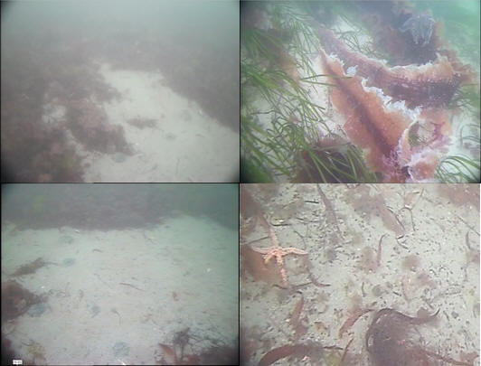
Video The benthic area surveyed by the video was complimentary to the side scan, providing a method of ground-truthing for the side scan sonar trace. The different video recordings were conducted using the REX ROV as well as a using a normal drop camera; these two systems produced high definition images as well as low moderate resolution images respectively. There were two camera drops conducted in the afternoon. The first camera drop started at 50°9’10.13N, 5°1’0.39 and ended at 50°9’16.08N, 5°0’52.42; the second camera drop was at 50°9’2.05N, 5°1’19.90W and ended at 50°9’10.07N, 5°1’11.02W. The ROV drop was at 5°00’55.5378W, 50°09’08.527, during its deployment, the recordings on board displayed coarse sand, seagrass, snakelock anemones and peacock worms. .The area surveyed by the video was used to confirm the findings of the side scan sonar results to create suitable habitat boundaries. Figure 2.4 shows some video stills from the ROV recording. The images obtained from the video results illustrate the different boundaries on the sea floor (see Figure 2.4; top left) as well as some fauna that were observed. From both the ROV and the camera drop, several different flora and fauna were observed. These ranged from maerl to seagrass beds; echinoderms, cuttle fish, small fishes and Arenicola marina mounds. |
Figure 2.4. Video stills from an ROV recording showing different sediment types, flora and fauna. |
||||||||||||||||||||||||||||||||||||||||||||||||||||||||||
| DISCUSSION | |||||||||||||||||||||||||||||||||||||||||||||||||||||||||||
|
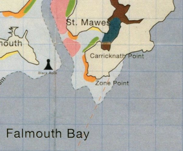
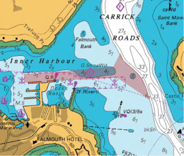
Maerl is a collective term for calcareous Rhodophyta, found in somewhat turbid waters of the European continental shelf, with different species dominating at different depths; Blunden et al. (1981) found that the species Lithothamnion corallioides and Phymatolithon calcareum predominate at up to 6m and from 6-10m respectively in the maerl beds at Falmouth. Maerl occurs in areas sheltered from intense wave action to prevent damage and dispersal into deeper waters, but a moderate water flow is needed to prevent burial by sedimentation (Hall-Spencer, 1998). The rhodoliths of maerl have incredibly slow growth rates of 0.1-1.0 mmy-1 in temperate waters, which means any damage to the habitat takes many years to recover (Bosence & Wilson, 2003). The complex nature of the rhodoliths and their skeletons provide multifaceted habitats harbouring high biodiversities of epifauna and infauna, which means they are comparable to seagrass beds for this reason (Grall & Hall-Spencer , 2003). The maerl provides an ideal sheltered nursery ground for many commercial species and broodstock bivalves, for example juvenile cod, king and queen scallops and juvenile pollack (Kamenos et al., 2004a; Kamenos et al. 2004b, Hauton et al., 2003; Hall-Spencer et al., 2003). Destruction of these habitats will therefore have a big impact on the local fishing industry as it decreases the number of juvenile fish restocking inshore areas, and so both maerl and eelgrass beds are in most need of conservation (Birkett, 1998). Falmouth Bay including the Fal and Helford, is designed a special area of conservation (SAC). SACs are strictly protected areas designed under the EC Habitat Directives. Maerl beds cover the mouth of the St Mawes harbour, whereas eelgrass beds such as Zostera marina beds cover the southern side of St Mawes harbor (Figure 2.5). In the Fal and Helford the largest maerl beds of England are found (Birkett, 1998). Fishermen have been dredging the sea floor of the Fal for oysters and scallop for centuries although both Maerl and Zostera are known to be easily damaged by dredging and ship anchors; as a result dredging has been restricted in certain areas of the Fal (Wathen, 2010). The Falmouth Cruise Project is a controversial new plan proposing to dredge a deeper and straighter new navigation channel from a depth of 5m depth at low tide to 8.5m at high tide. The channel from Carrick Roads to the Queens and Northern Wharves will create a continuous deep water berth to allow cruise ships into Falmouth bay (Figure 2.6). So far the plan has been blocked by the Marine Management Organisation (MMO), but slackening by the government of how the EU habitat directive is applied could mean that this project (along with other similarly environmentally destructive plans) could be implemented. The ramifications of this project going ahead will mean a significant loss of viable maerl habitat, with a net maerl bed loss of a predicted 4 hectares (Falmouth Cruise Project, 2008). Computational modelling has predicted that the sediment plume created from the silt curtain dredging will move west of the dredging area and therefore should not affect the live maerl bed and seagrass beds to the east and north of the channel. However, any mistakes in the dredging might have a significant impact on the seagrass and live maerl beds to the east, and so habitat mapping is vital in these areas to monitor the possible impact of the dredging project. De Grace et al. (2000) stated that the slow growth rate of maerl beds means that any sedimentation impedes recolonization and growth. As both maerl and seagrass require a large amount of light to photosynthesise efficiently, the likely impact of the plume would devastate these important community structuring elements. Maerl is also important to monitor as it contributes significantly to the global distribution of calcium carbonate budgets and is one of the fastest carbonate producing marine organisms, depositing large amounts of biogenic calcium carbonate (Vecsei, 2001; Bosence, 1980). The generated benthic habitat map that was created using a combination of the side scan data, complimented by the ROV and camera trawl ground-truthing, and provided a good insight into the different habitat types in the St Mawes area. Our habitat map generated 8 different habitat zones, 5 of which could be confirmed using video data, and each of 5 matched the proposed St.Mawes area of the Fal & Helford Marine SAC habitat map (Figure 2.5). Both our generated map and the Fal & Helford Marine SAC Habitat map indicate a heavy amount of eelgrass bedding to the east of the surveyed area (confirmed using the ROV high definition video). This is because of the metamorphic rock bedrock outcropping close to the shore, which provides a substrate for the eelgrass to attach to (Leveridge et al., 1990). The time viewed on the video at which the transition from maerl to maerl and sand at around 184,325m E, 32,325m N, then to patchy seagrass at around 184,400 E, 32,350 N matched the transition locations on the sidescan data, again in the same area to the Western side of the transects described by the Fal & Helford Marine SAC habitat map. At the point around 184,700 E, 32,400 N, on the northern side of the transect area there was a transition to macroalgae, with a marked change in texture on the side scan trace matched by the change observed in the camera trawl. There were several limitations during the benthic habitat process, namely, the lack of sediment grabs which would have provided a far greater insight as to the habitats living in the benthos. Many species cannot be identified by a simple video trawl, especially infauna such as polychaetes and smaller species that may not have been visible at the resolutions used, and so the ground-truthing would have been far more effective with the inclusion of this data. Although sediment grabs are damaging to the maerl environment, these could have been replaced by an exploratory dive, to preserve the live maerl but also identify a wider variety of species. The turbidity of the water had a marked effect on the video trawls which again made identification difficult. Another limitation of the benthic habitat mapping process was the quality of data provided by the side scan – there were artefacts in the side scan trace which may have meant distinguishing between bedform and habitat types was difficult, as some differences in texture of the side scan trace were generated by the side scan itself. |
Figure 2.5. SACs in St. Mawes harbour and Falmouth Bay |
||||||||||||||||||||||||||||||||||||||||||||||||||||||||||
|
Figure 2.6. Location of proposed new navigation channel (purple) |
|||||||||||||||||||||||||||||||||||||||||||||||||||||||||||
| BACK TO TOP | INTRODUCTION | EQUIPMENT | ESTUARY |
|
| BACK TO TOP | INTRODUCTION | EQUIPMENT | OFFSHORE | REFERENCES |
| ESTUARY | ||||||||||||||||||||||||||||||||||||||||||||||||
| AIM | ||||||||||||||||||||||||||||||||||||||||||||||||
|
To develop an understanding of how the Fal estuary acts physically, chemically and biologically as a temporal and spatial transition zone between the freshwater inputs and the coastal seas. |
||||||||||||||||||||||||||||||||||||||||||||||||
| INTRODUCTION | ||||||||||||||||||||||||||||||||||||||||||||||||
|
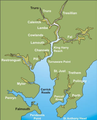
In estuarine systems, a balance is struck between the input of fresh water from the riverine end and extent of tidal mixing from the seaward end. In many estuaries, the water tends to be stratified to varying degrees due to less dense freshwater sitting above the higher density seawater. The extent of this stratification depends on many variables including but not limited to: the strength and direction of tidal currents, the fresh water flux and the amount of turbulence in the water column (wind driven mixing etc.). Nutrient inputs into an estuarine system include river water inputs, addition of aerosols and ground water, all of which can have both natural and anthropogenic sources. For some nutrients, estuaries simply behave as a chemically conservative mixing interface between rivers and the ocean. For others, chemical and biological reactions may take place within the estuary to either add or remove certain constituents (Loder and Reichard, 1981). It is therefore important to understand the processes involved during the transportation of nutrients through an estuary as the consequences affect phytoplankton growth, local production as well as chemical cycling. The area of interest - Fal estuary is known as a ‘ria’, or drowned river whereby a rise in sea level causes the valley to become flooded (Figure 3.1). The freshwater inputs of the estuary include the River Truro, the River Kennal, the River Penryn and the River Carnon. The seaward end of the estuary is connected to the Western English channel, a shelf sea that commonly shows frontal systems. |
Figure 3.1. Diagram illustrating how the local geography of the Fal area has changed over the last 18,000 years. Left: the Devensian per glacial conditions when sea levels were much lower. Right: the end of the ice age after sea levels rose to present levels and the Fal valley system was flooded forming the estuary seen today (Bird E, 2000) |
|||||||||||||||||||||||||||||||||||||||||||||||
| METHOD | ||||||||||||||||||||||||||||||||||||||||||||||||
|
The fieldwork was carried out on the 2nd of July 2012 and involved periodic time series measurements from a pontoon at King Harry Passage (50°12’57.97 N, 005°01’39.52 W) as well as spatial measurements taken from aboard the R.V. Bill Conway starting at Woodbury Point at the head of the river and ending at Saint Just Pool near the end of the estuary. On the pontoon, samples were taken about every fifteen minutes beginning at 09:00 UTC until 11:15 UTC then again from 12:05 UTC to 15:15 UTC using 3 different instruments. First a YSI multiprobe which gave a measure of depth, temperature, salinity, fluorescence, pH, and oxygen saturation. Second, a current meter was used to give current velocity and direction at depth. Velocities were recorded on both the down and the up casts and averaged due to the variability in the values given by the sensor. Finally, an irradiance meter was used to measure light levels at depth. This gave a spectrum of measurements across low tide, the flood and high tide. Separate chlorophyll samples were taken directly from the water using filters. While onboard R.V. Bill Conway, a total of eight transects were taken using the ADCP, Acoustic Doppler Current Profiler. The first four transects were taken at between the head of the river down to the location of the pontoon. Transect five was taken at the site of the pontoon then the final three transects were taken in the lower end of the estuary. A total of five CTD; conductivity, temperature and depth, vertical profiles were made along the entirety of the path of the vessel. The CTD recorded the depth, temperature, salinity, fluorescence, and transmission but no Niskin bottles were attached to the system due to fault in the launching mechanism. Because the CTD could not launch Niskin bottles, bottles were deployed from a hydroline to retrieve discrete water samples for phosphate, nitrate, silicon, dissolved oxygen and chlorophyll. Attached to the niskin bottle on the hydroline was a TS probe and depth sensor for accurate recording. Three plankton samples were also taken by dragging a plankton net consisting of a mesh size 200microns for five minutes behind the vessel. |
||||||||||||||||||||||||||||||||||||||||||||||||
|
|
|||||||||||||||||||||||||||||||||||||||||||||||
| CONTOUR PLOTS | ||||||||||||||||||||||||||||||||||||||||||||||||
|
Contour plot of current velocities (Figure 3.2): The graph shows a peak in current velocity of around 0.4m/s between 12:00 and 14:00gmt, in the middle of the high and low tides at 15:50 and 10:05gmt respectfully. This is indicative of a standing tidal wave where current velocities tend to their maximum a quarter of a period after high / low tide due to the summation of the wave and its reflection. Contour plot of Temperature (Figure 3.3): The graph shows homogeneity with respect to temperature throughout the water column at the pontoon across time, however as it progresses from low to high tide, the temperature decreases from around 15.5°c to 14.0°c . This is due to the cooler seawater moving up the estuary with the tides. Contour plot of salinity (Figure 3.4): Around low tide, the water column appears to be stratified with fresher water on top at around 25psu and denser saltier water at depth of around 30psu, possibly due to the flux of freshwater being relatively high compared to the tidal mixing. As it approaches high tide the water column salinity increases to 34psu and becomes more homogenous. This is as sea water is pushed up the estuary and tidal mixing increases which acts to increase mixing between the relatively decreasing freshwater flux and the seawater being pushed up the estuary. Contour plot of chlorophyll (Figure 3.5): Higher chlorophyll concentrations of >6.0mg/m^3 appear mainly above 2m indicating that the phytoplankton maintain denser populations at the surface for photosynthesis. However the dense areas are patchy, reflecting the natural variability in biological data. Contour plot of oxygen saturation (Figure 3.6): Across the recorded period, oxygen saturation is less at depth where it is consumed by heterotrophic activity than at the surface, where oxygen can readily diffuse in from the atmosphere, a difference of around 2-4%. With respect to the tides, oxygen saturation increases as high tide approaches. This is because the tide carries well mixed sea water with higher oxygen levels then riverine water up the estuary, increasing oxygen saturation by around 4%. |
Figure 3.2. Current velocity contour plot |
Figure 3.3. Temperature contour plot |
||||||||||||||||||||||||||||||||||||||||||||||
|
Figure 3.4. Salinity contour plot |
Figure 3.5. Chlorophyll contour plot |
|||||||||||||||||||||||||||||||||||||||||||||||
|
Figure 3.6. Oxygen saturation contour plot |
||||||||||||||||||||||||||||||||||||||||||||||||
| CTD | ||||||||||||||||||||||||||||||||||||||||||||||||
|
The CTD profiles from Station 1 show that in general temperature decreases with depth. There is a thermocline at around 1.5m, where the temperature decreases from around 15.4˚C to just above 15˚C at a depth of 14m. There was a more gradual increase in salinity from around 20 at the surface to around 30 at depth. This decrease is gradual, apart from at between the depths if 0.25-0.75m, where the salinity does not appear to change. The higher temperature waters, lower salinity waters in the upper layer of the water column are less dense than the colder, saltier water below it. This less dense water may be the river water sitting above seawater. The seawater signal will be the weakest at this station, as it is the furthest from the mouth of the estuary. Furthermore, the seawater entering the upper part of the estuary will be less saline, due to mixing with the upper freshwater layers.
The
fluorescence peaks at the surface, and then generally decreases
slightly with depth. The data is however quite erratic. The peak in
fluorescence may be caused by large numbers of phytoplankton in
surface waters caused by higher irradiance. The general patterns at station 4 are similar to previous stations, however there is a clear thermohalocline at 2m, due to a layer of river water above the seawater. At these four stations, the thermocline is mainly caused by differences in salinity. At station 5, temperature still decreases at depth, but there is a thermocline between 4m and 8m. Salinity appears to be fairly constant throughout the water column. The fluorescence peak is deeper, between 2m and 4m. This roughly corresponds to the thermocline , which is where nutrients are present, and where a high enough level of sunlight is present to allow photosynthesis. At site 6 (no discrete water sampling for chemical analysis was conducted here), temperature decreases with depth and salinity increases, with two thermohaloclines, at 4m and 9m. Fluorescence values remain relatively constant throughout the water column. Stratification at these two sites is mainly due to temperature differences. |
 CLICK TO ENLARGE Figure 3.7. Station 1 |
 CLICK TO ENLARGE Figure 3.8. Station 2 |
||||||||||||||||||||||||||||||||||||||||||||||
 CLICK TO ENLARGE Figure 3.9. Station 3 |
 CLICK TO ENLARGE Figure 3.10. Station 4 |
|||||||||||||||||||||||||||||||||||||||||||||||
 CLICK TO ENLARGE Figure 3.11. Station 5 |
 CLICK TO ENLARGE Figure 3.12. Site 6 |
|||||||||||||||||||||||||||||||||||||||||||||||
| PHOSPHATE | ||||||||||||||||||||||||||||||||||||||||||||||||
|
Station 1 was the northern most sample site in the Estuary and follows a general pattern of increasing Phosphate concentrations with decreasing depths, only being the more severe than the other stations. This trend with increasing concentration in the upper water depths, slowly weakens as the stations moved down the estuary. Eventually ending at station 5, that displays a Phosphate concentration that is almost equal within the water column. Phosphate is generally higher in fresh water because it comes mostly from the organic matter of decaying plants and other run-off sources. Being so, it can be determined that the further North within the estuary, should have the highest phosphate levels. Data began recording at the top of the estuary at low tide and ended at the bottom at high tide. When data initially began, there is very little mixing occurring and a high source of phosphate input therefore it is expected to see a higher degree of changes with depth as in stations 1 and 2. As the day went on and the tide came in, mixing began to occur leading to a more evenly distribution of phosphate concentration in the water column. |
CLICK TO ENLARGE Figure 3.13. Phosphate depth profile |
|||||||||||||||||||||||||||||||||||||||||||||||
| DISSOLVED OXYGEN | ||||||||||||||||||||||||||||||||||||||||||||||||
|
In general, the dissolved oxygen level should be the highest near water surface and decrease with depth due to increase of space in the water column and biological respiration. The O2 saturation of station1, 2, 3, and 4 are around 100% at the water surface. From that point, O2 saturation of each station behaved differently. In shallow water station 1, dissolved oxygen level decreased with depth. Similar behaviour was observed at station 5, but O2 saturation level is significantly higher than all other station. This maybe due to the strong tidal mixing at the frontal line providing ideal environment for plankton species. At any depth of any station, the increase of O2 saturation indicates an increased number of phytoplankton in the water column. This is observed at station 3 at the depth of 2m, and at station 5 at the depth of 4m. Phytoplankton data does not correlate with oxygen saturation level. This maybe due to grazing and rainfalls observed on the sampling day. |
CLICK TO ENLARGE Figure 3.14. Dissolved oxygen profile |
|||||||||||||||||||||||||||||||||||||||||||||||
| PLANKTON | ||||||||||||||||||||||||||||||||||||||||||||||||
|
Phytoplankton (Figure 3.15) All three stations measured were dinoflagellate and diatom dominated. Station three has a much higher concentration in phytoplankton, suggesting that this area is more productive at the time of data collection. Ciliates are almost completely absent from all three stations, possibly indicating that high motility is not as advantageous in this environment. At station one, dinoflagellates were dominate suggesting that mixing of the estuary was occurring. Whereas stations three and five had a majority of diatoms. Zooplankton (Figures 3.16 - 3.19) Zooplankton abundance should be compared to phytoplankton abundance as they each are reliant upon the other. Zooplankton feed upon phytoplankton, therefore theoretically following the same trends. However, there are fewer zooplankton at station one than at station three and five. Station three has greater equitability. Copepods are the most dominant in all three stations as they are the most abundant species on Earth. |
Figure 3.15. Phytoplankton taxa occurring in the estuary |
|||||||||||||||||||||||||||||||||||||||||||||||
 CLICK TO ENLARGE Figure 3.16. Zooplankton species abundance |
 CLICK TO ENLARGE Figure 3.17. Zooplankton species at station 1 |
|||||||||||||||||||||||||||||||||||||||||||||||
 CLICK TO ENLARGE Figure 3.18. Zooplankton species at station 3 |
 CLICK TO ENLARGE Figure 3.19. Zooplankton species at station 5 |
|||||||||||||||||||||||||||||||||||||||||||||||
| CHLOROPHYLL | ||||||||||||||||||||||||||||||||||||||||||||||||
|
The chlorophyll graph (Figure 3.20) displays the concentration with depth in the estuary at all five stations. Station one was taken at the northern most point while station five was nearest to the mouth of the estuary. Station one through four are very similar results of the highest chlorophyll concentrations at surface waters with a decreasing concentration with increasing depth. |
CLICK TO ENLARGE Figure 3.20. Chlorophyll depth profile for stations in the estuary |
|||||||||||||||||||||||||||||||||||||||||||||||
| CONCLUSION |
|
The Falmouth Field Course took place over a two week period where students underwent three different disciplines related to the Fal Estuary. These disciplines included geophysics, offshore and estuary. Students were then task to take the raw data obtained from these practicals and transformed them into useable data for a final report. For the offshore discipline, students were tasked with testing the different concentrations of nutrients within the water column. The surface nutrients were found to be higher at the mouth of the estuary due to the influence of the riverine input. Also, it was revealed that there was a higher plankton concentration in the upper water column which roughly corresponds to the 1% light depth. From the data analysed, it showed that the vertical mixing processes can have some influence on the structure and functional properties of plankton communities. Lastly, the zooplankton distribution followed the phytoplankton distribution showing that the main control or limitation is food supply. From the estuary data provided it was revealed that the estuary behaved as per a normal estuary. The nutrients levels were noticeably higher because it was a riverine end member as compared to the offshore data. There were some nutrients in the estuary that were behaving both conservatively and non-conservatively throughout the estuary. This could have been due to their addition and removable from the estuary as a result of various processes mainly for their use as food resources. For the geophysics practical, this was done through the use of side scan sonar technology, drop cameras and a remotely operated vehicle. However, despite the use of such technology to get a view of the benthic habitats, there were some limitations in confirming what was being recorded. The main limitation, lack of sediment grabs, was prohibited due to new laws that require a permit for such activities. Since of the sediment grab could not be used it limited the identification of many flora and fauna on the seafloor. Also, a major limitation was the results produced from the side scan, this discrepancy in results meant that the benthic habitat mapping process would be hinder. Despite these limitations however, a suitable map was created that displayed to the best possible idea of the benthic community. The Fal Estuary is protected under the new conservation policy by Join Nature Conservation Committee. Due to this new registration, we were not able to use grab sampling method. Our habitat mapping was carried out mainly by utilizing GeoAcoustic Digital Side Scan Sonar and ROV REX, which provided us high resolution image of the seafloor. 10um nitrate and 10um nitrate sample through FLA, all Nitrate was successfully reduced to Nitrite. However, due to problems with the sampling injection technique into the spectrophotometer (air bubbles caught in the tubing cause huge deviations in results produced) along with the very low nitrate levels being mainly below the detection level of the standards provided, nitrate data was not recorded for the samples provided. As we design this webpage, we decided to keep the website as simple as possible to highlight the important information. Therefore, our website does not describe the specific feature of each equipment and vessel. THE VIEWS AND OPINIONS EXPRESSED ON THIS WEBPAGE DO NOT REPRESENT THE VIEWS OF THE UNIVERSITY OF SOUTHAMPTON OR THE FALMOUTH MARINE SCHOOL |


.JPG)
.JPG)