![]()
![]()
![]()
![]()
![]()
![]()
![]()
![]()
![]()
![]()
![]()
![]()
![]()
![]()
![]()
![]()
![]()
![]()

|
James Fay Denise Herrera Alex Martin Marcus Militello Davey Peyton |
 |
Sion
Roberts Bryony Snooks Ellie Stacey Emma Whelan |
| Introduction | |||||||||||||||||||||||||||
|
Falmouth is located at the mouth of the river Fal, on a headland (the Roseland peninsula) in South Cornwall. The river Fal has many tributaries, including the Truro river as its main tributary, leading into the estuary with varying amounts of anthropogenic impact, such as the extreme levels of pollution, which can be seen at Restronguet creek. The pollution at Restronguet creek can mainly be attributed to the Wheal Jane tin mine at Chacewater, which leaked “50 million litres of acidic metal laden water into Restronguet creek” in 1991 (Exeter University, n.d.). The Fal estuary itself is a ria system covering about 2500ha of which about a third is intertidal and has a tidal range of more than 5m placing it in the macrotidal (Pirrie et al, 1997). It is one of the largest natural harbours in the world and so experiences a large amount of shipping every year with large container ships reaching high up into the river. Due to its picturesque setting and the natural harbour it is an asset to the local economy through tourism (Macadam et al, 2003). The Fal and Helford estuaries together form a special area of conservation covering various habitats from marine habitats to tidal river habitats and a total area of almost 6400ha (JNCC, 2000). All times are in GMT, all grid references WGS84. |
|
||||||||||||||||||||||||||
| Vessels | ||||||||||||||||||||||||||||||||||||||||||||
| Callista |
Bill Conway |
Grey Bear | ||||||||||||||||||||||||||||||||||||||||||
|
The R.V Callista is a 19.75m research catamaran. It can operate for a maximum of 30 hours at economy speed up to a maximum of 60 miles offshore. It has dry and wet labs and a large aft deck. The rear A-Frame has a max lifting limit of 4 tonnes.
|
The Bill Conway is an 11.74 m research vessel based at the National Oceanography Centre, Southampton. It has a maximum range of 60 miles offshore.
|
The Grey bear is a manoeuvrable and stable boat able to perform in a multi-role capability with a range of 20 miles.
|
||||||||||||||||||||||||||||||||||||||||||
| Equipment | ||
| Name | Description/Uses | Image |
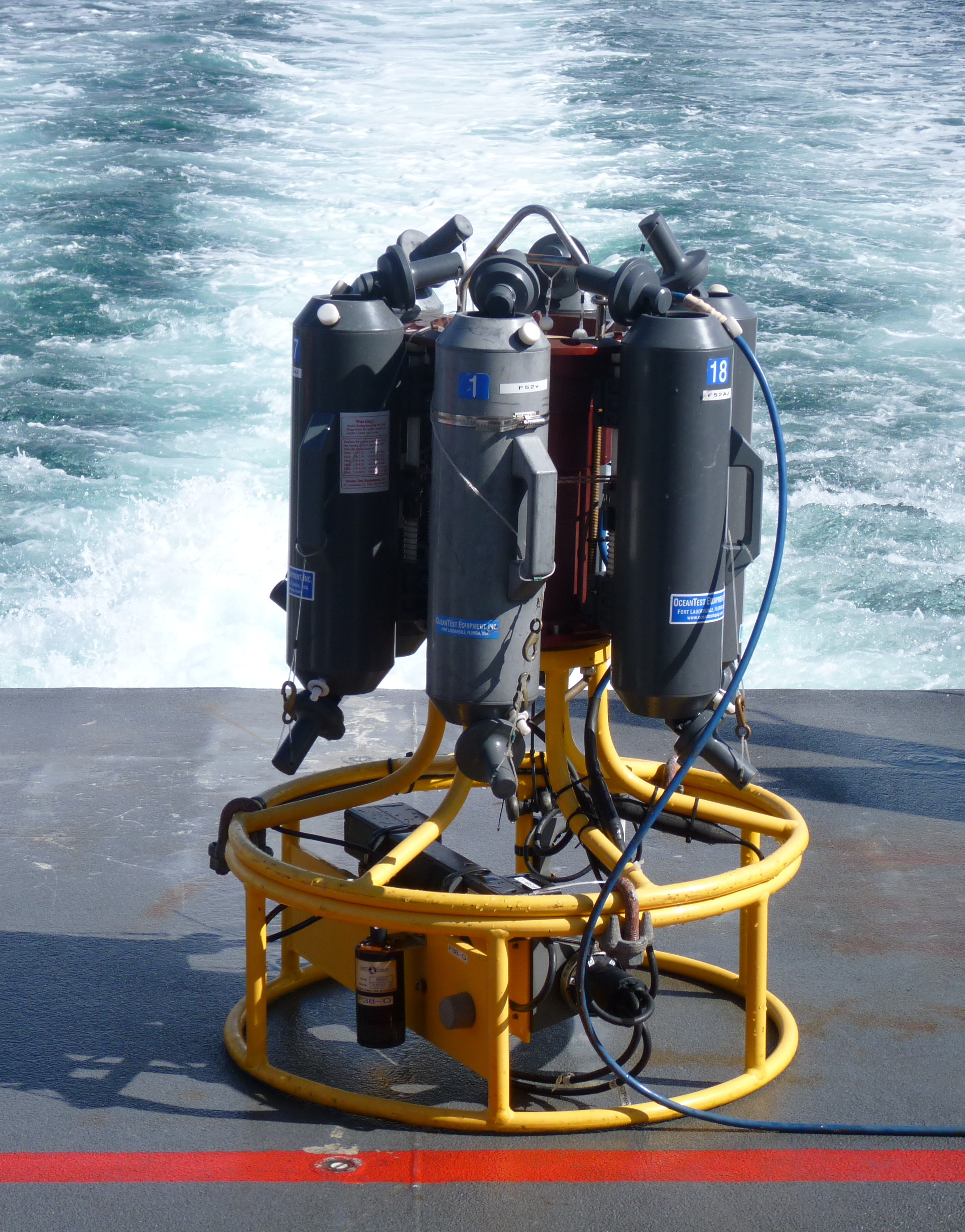
| CTD |
A CTD is an instrument package which can measure the conductivity (salinity) and temperature of seawater and record the depth at which it is sampling. The CTD can house a variety of sensors and a water bottle rosette in addition to measuring temperature and salinity. The CTD used for our offshore boatwork supported a 6 Niskin bottle rosette and a range of sensors including a fluorometer, transmissometer, platinum resistance thermometer and a light sensor. Data is sent electronically to the ship via a conducting cable which is attached to the top of the CTD. |
 |
| Niskin Bottle | A Niskin bottle is a plastic bottle which has a spring loaded mechanism to shut both ends of the bottle at a required depth. In our offshore practical work, six 6-litre Niskin bottles were attached to a CTD rosette and were shut electronically via the conducting cable connecting the ship to the CTD. Niskin bottles allow water samples to be taken from a variety of depths during a CTD vertical profile. The bottles were shut at depths of interest, which were determined by looking at the temperature and salinity measurements recorded by the CTD. | |
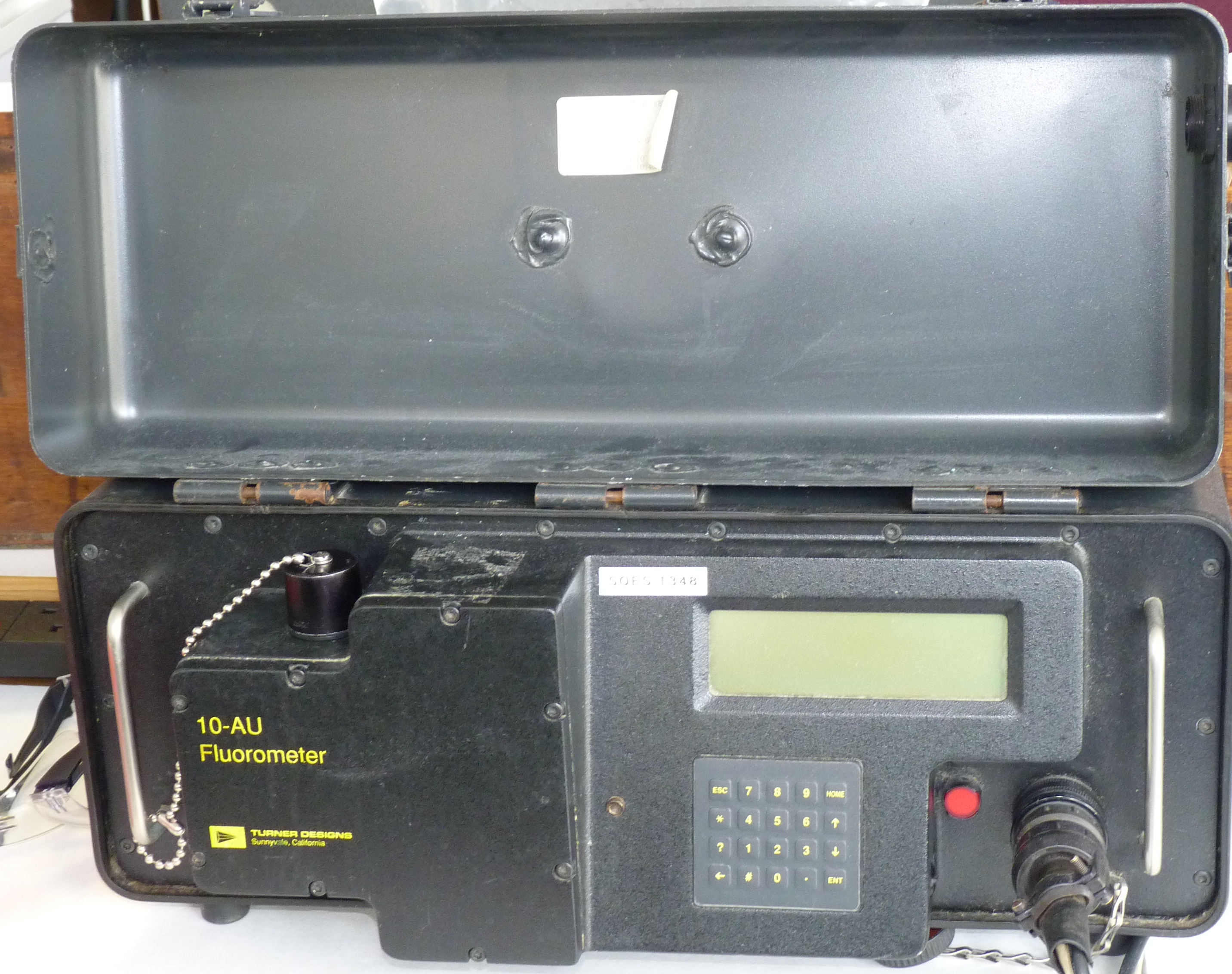
| Fluorometer |
A fluorometer is an instrument to measure chlorophyll concentration by transmitting a blue light excitation beam which causes the chlorophyll to fluoresce and the instrument outputs a value of fluorescence in voltage. In both offshore and estuarine practicals it was attached to the rosette frame on the CTD, making it possible for us to get a vertical profiles of chlorophyll concentration. |
|
| Transmissometer |
A transmissometer measures the attenuation of a light beam which is shone from one end of the instrument to the other. The distance between the output end and the receiving end varies with the type of water body being sampled. For example, in very turbid estuaries, the distance between the two ends is shorter i.e- 10cm as it is a very turbid environment and the light attenuates quickly. The opposite is true for very clear, calm waters such as those found in the tropics. |
|
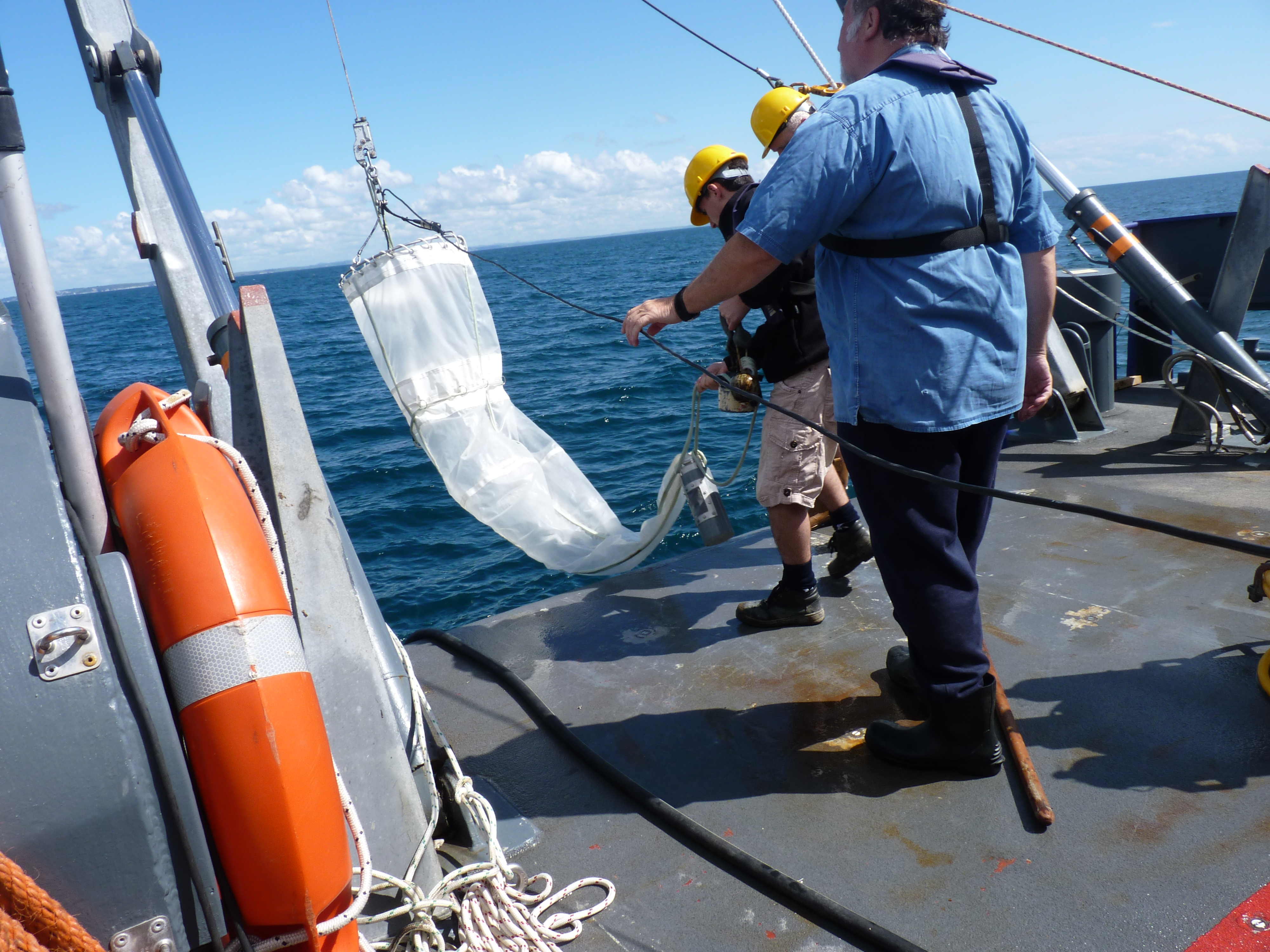
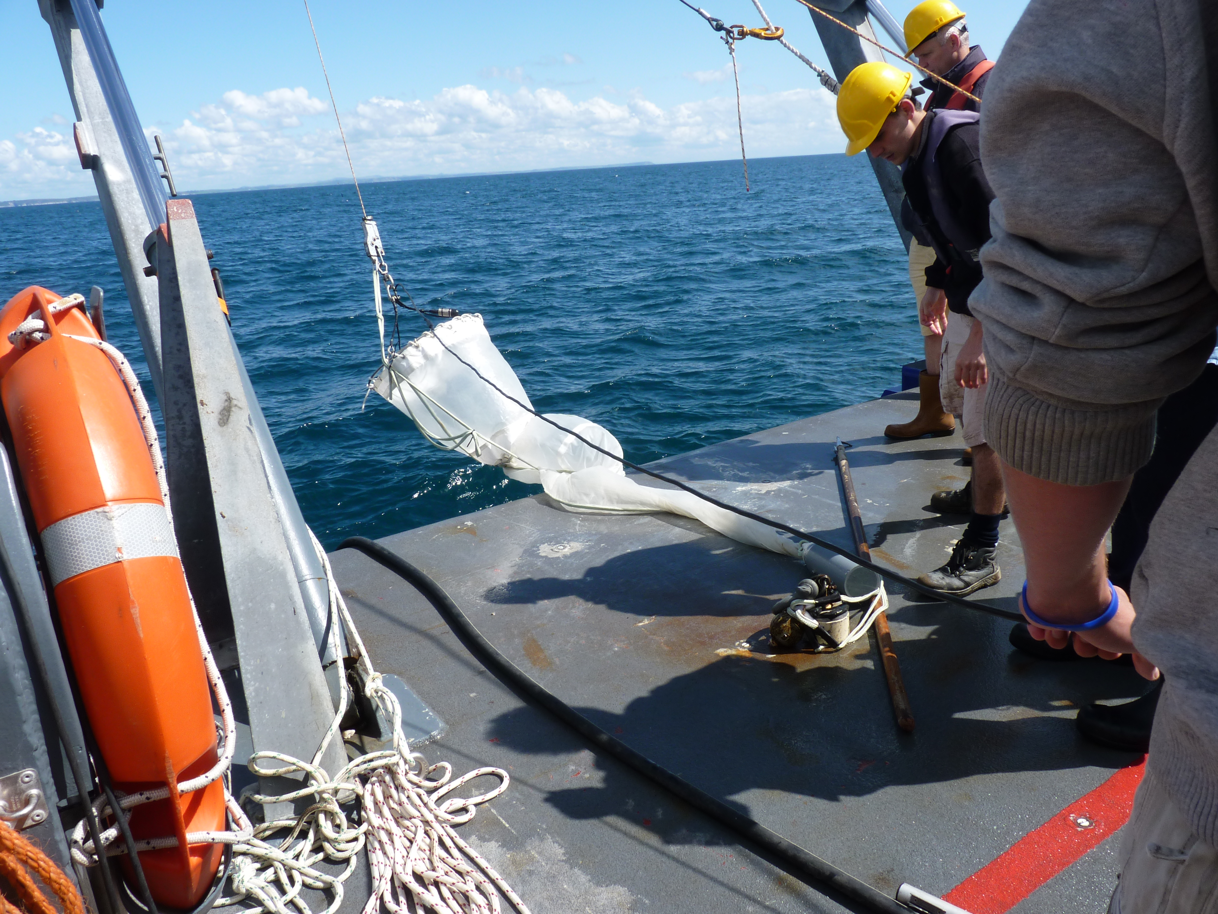
| Plankton Net |
Plankton nets are net funnel structures designed to collect planktonic organisms intact which are towed behind research vessels. Often, flow meters are attached to the net to give an indication of the volume of water funneled. The size and type of specimens collected can be dictated by the mesh size. In our offshore experiment, a ring plankton net was used with a 200micron mesh size and 0.6m diameter. At the end of the net there is a collection bottle, in which plankton smaller than the mesh size are collected. |
 |
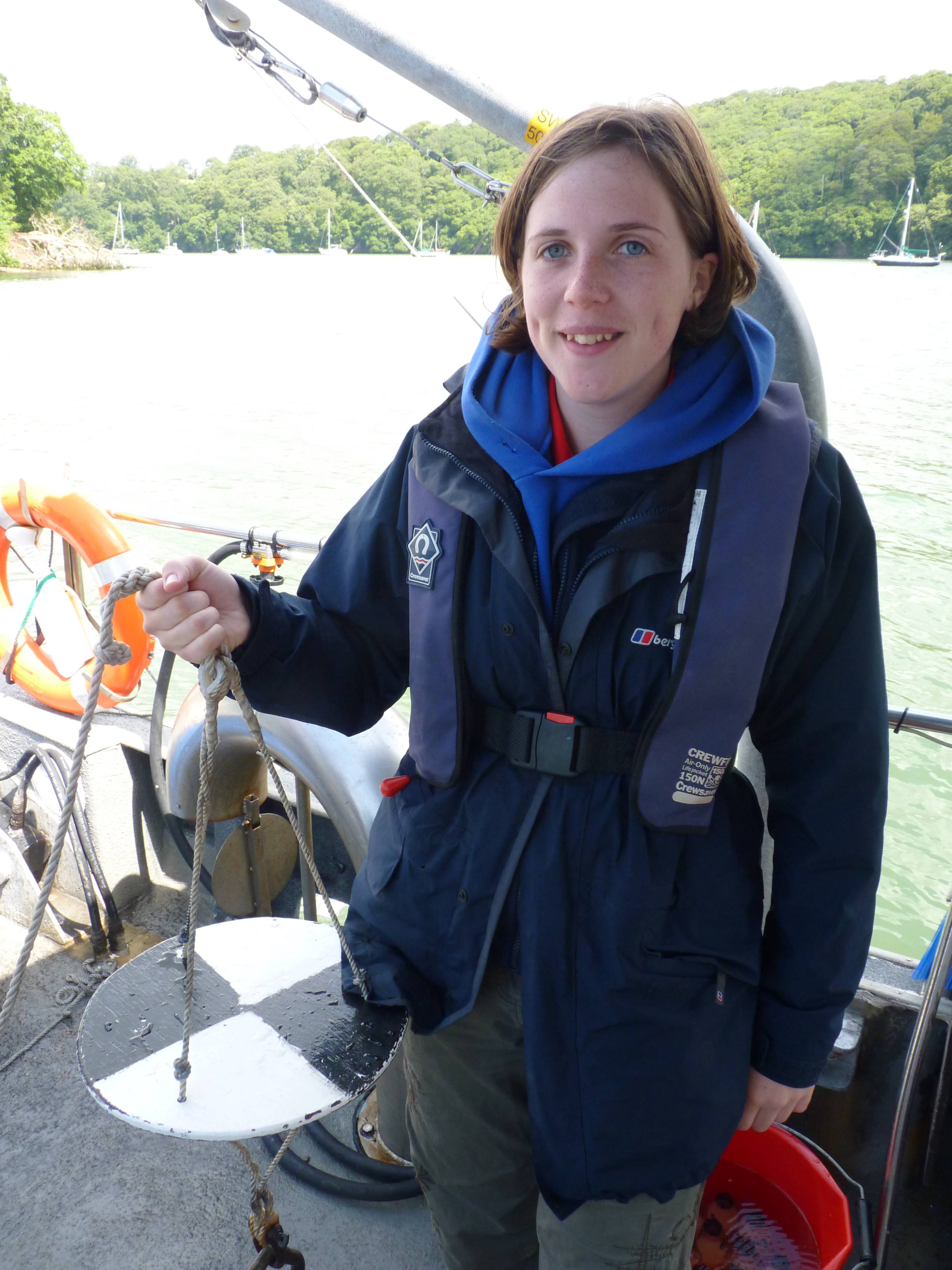
| Secchi Disk |
A Secchi disk is a weighted circular black and white plate that estimates quantitatively the amount of light at different depths within the water column. From these measurements, the light attenuation co-efficient, k, and an estimate of the euphotic zone (three times the Secchi disk depth) can be calculated. The Secchi disk is a very subjective method and judgment of when the disk can no longer be seen can differ. Factors such as amount of suspended particulate matter, both organic and inorganic, can increase light attenuation, as well the angle of incident light, the amount of phytoplankton and turbidity. |
 |
| Sidescan Sonar |
Sidescan sonar equipment is deployed on a towfish which is towed behind the research vessel. Sidescan sonar works on the principal of sonar pulses being released from a transducer on the towfish at a particular frequency. In our geophysics practical the towfish pulsed at a 110 kHz which is a low frequency. High frequency sonar can also be used (315 kHz), which outputs a very high resolution trace, but the swath is smaller and hence the range is limited. Once the pulses have been outputted by the receiver, the receiver on the towfish receives return pulses where the sonar has been reflected from objects. Pulses are returned from the water column, benthic flora and fauna, bedform features, anthropogenic and natural objects. The strength of the return pulses and the time lag between the pulse being sent and received allow a Sidescan trace to be produced. From this trace, the height of bedform features, the water column, sediment type and characteristics, anthropogenic features such as moorings, anchorings and ship wrecks can also be identified. |
 |
| Video Camera |
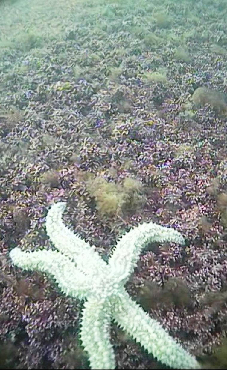
Video cameras can act as complimentary equipment to Sidescan surveys or can be used extensively to map large areas of benthic habitats. They can be towed behind a moving vessel or lowered down through a vertical profile of the water column. The video cameras allow accurate taxonomic identification of species, which might otherwise be missed or damaged in VanVeen grabs. Another advantage is the video camera can accumulate data over a larger area compared to grabs. The cameras can also have an integrated scale so when the footage is replayed accurate size estimates of the flora and fauna can be attained. |
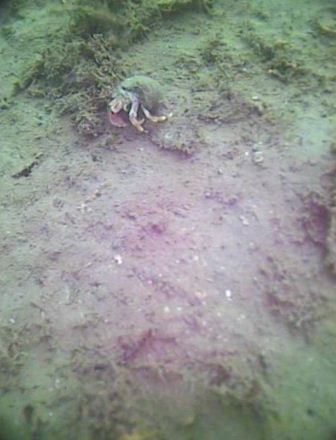
Image from video of sea floor at grab site 2 showing Pagurus bernhardus. |
| T-S Probe |
T-S (Temperature and salinity) probe measures the conductivity of the water to give us a salinity reading and uses a thermistor to measure the temperature of the water column. The sensors are positioned at the base of the probe and data is sent back electronically to the vessel via an electronic cable. T-S probes are predominantly lowered vertically down through the water column, so the water column thermohaline structure can be identified. The main aim of our offshore boatwork was to sample on either side of the thermal front. A T-S probe was kept permanently submerged in a bucket, supplied with surface water. The probe was used predominantly as an indicator of which side of the front we were and to indicate places of interest where we may need to sample. |
|
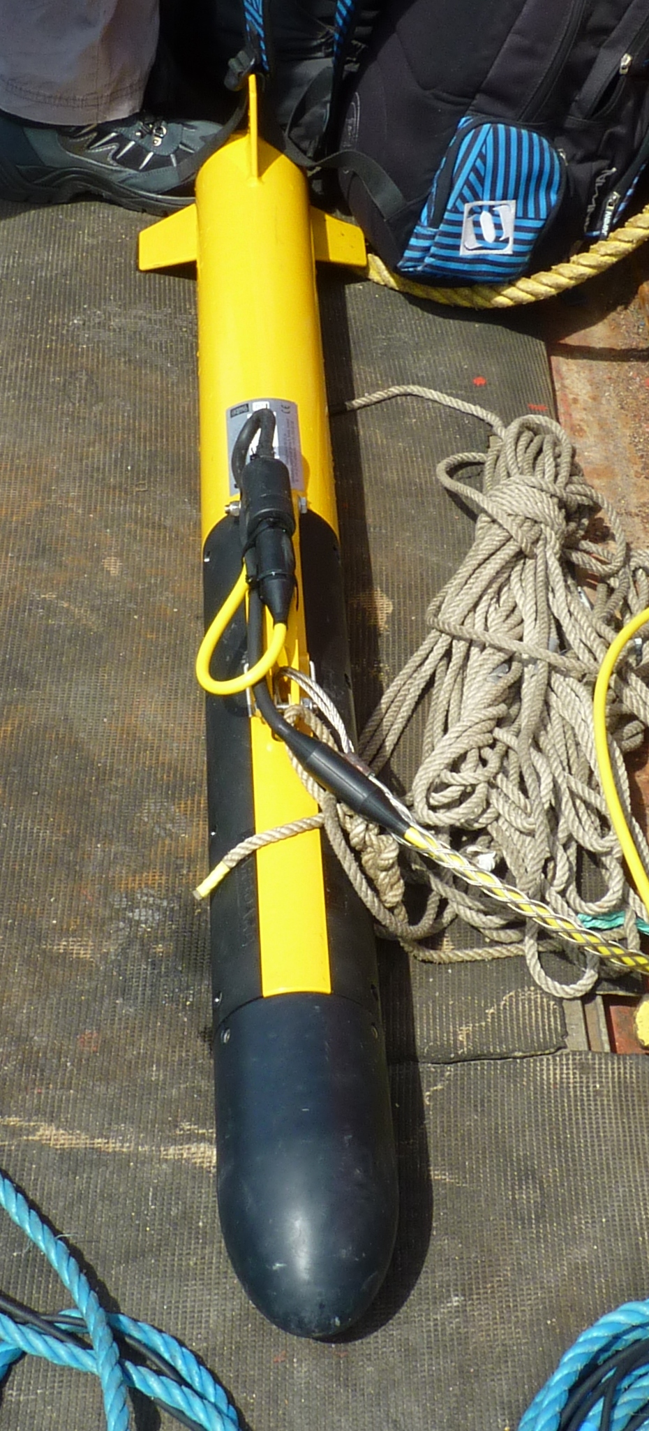
| ADCP |
An Acoustic Doppler Current profiler uses sound to quantify water velocities, magnitude shear, backscatter and current direction at different depths in the water column. The ADCP has both a transducer which sends out the pulses and a receiver which receives the returned pulses. By using four beams and the concept of the Doppler shift, all the listed parameters can be measured. |
 |
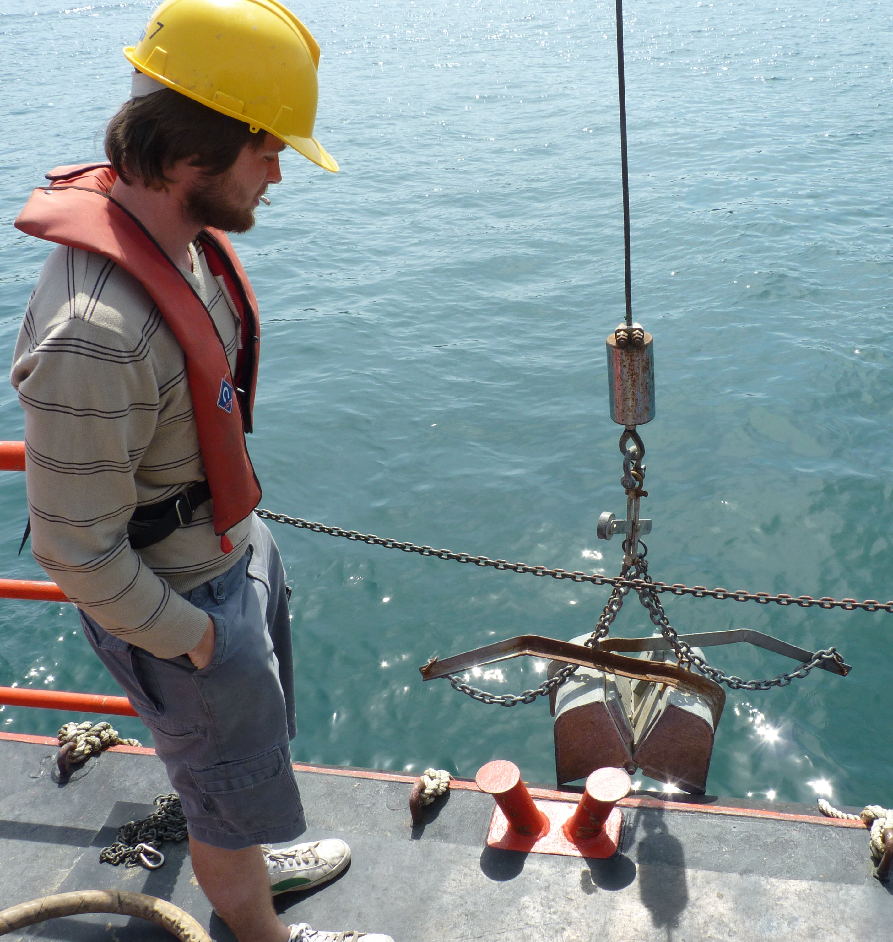
| Van Veen Grab |
The grab is connected to a crane which deploys the grab vertically down the water column. When the grab hits the seafloor, a change in tension initiates a mechanism to close the grab. This encloses both benthic flora and fauna and benthic sediments. Once the grab has been recovered, sediment type and characteristics can be measured and organism identified. The grab acts as a qualitative estimate of organic and inorganic characteristics of the benthos. |
 |
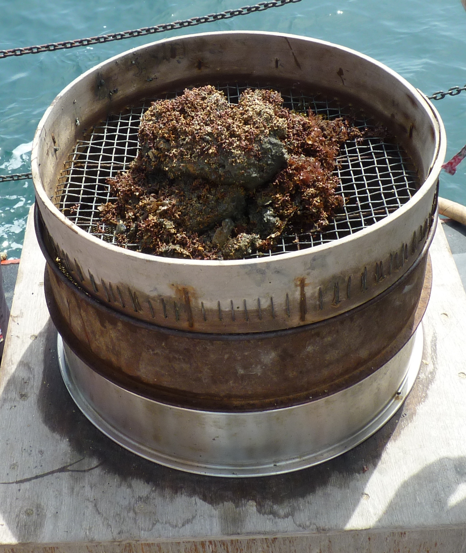
| Sieve Stack |
Sieve stacks were used on the offshore boat to aid separation of the grab material collected. We used three sieves in a stack with decreasing mesh size down the stack: 10mm,2mm and 1mm. |
 |
| YSI probe |
The YSI probe is a multi-parameter probe that simultaneously measures dissolved oxygen, pH, conductivity and temperature. On our estuarine practical, the YSI probe was used to measure the temperatures and salinities of the water collected in the Niskin bottles from the CTD at specific depths at each station. This data allowed calibration of the CTD thermometer outputs and also was used to calculate % oxygen saturation using the Winkler method.
|
image from www.ysi.com |
| Lab & Collection Methods | ||
| Collection & Wet Lab Based Preparation on Boats | ||
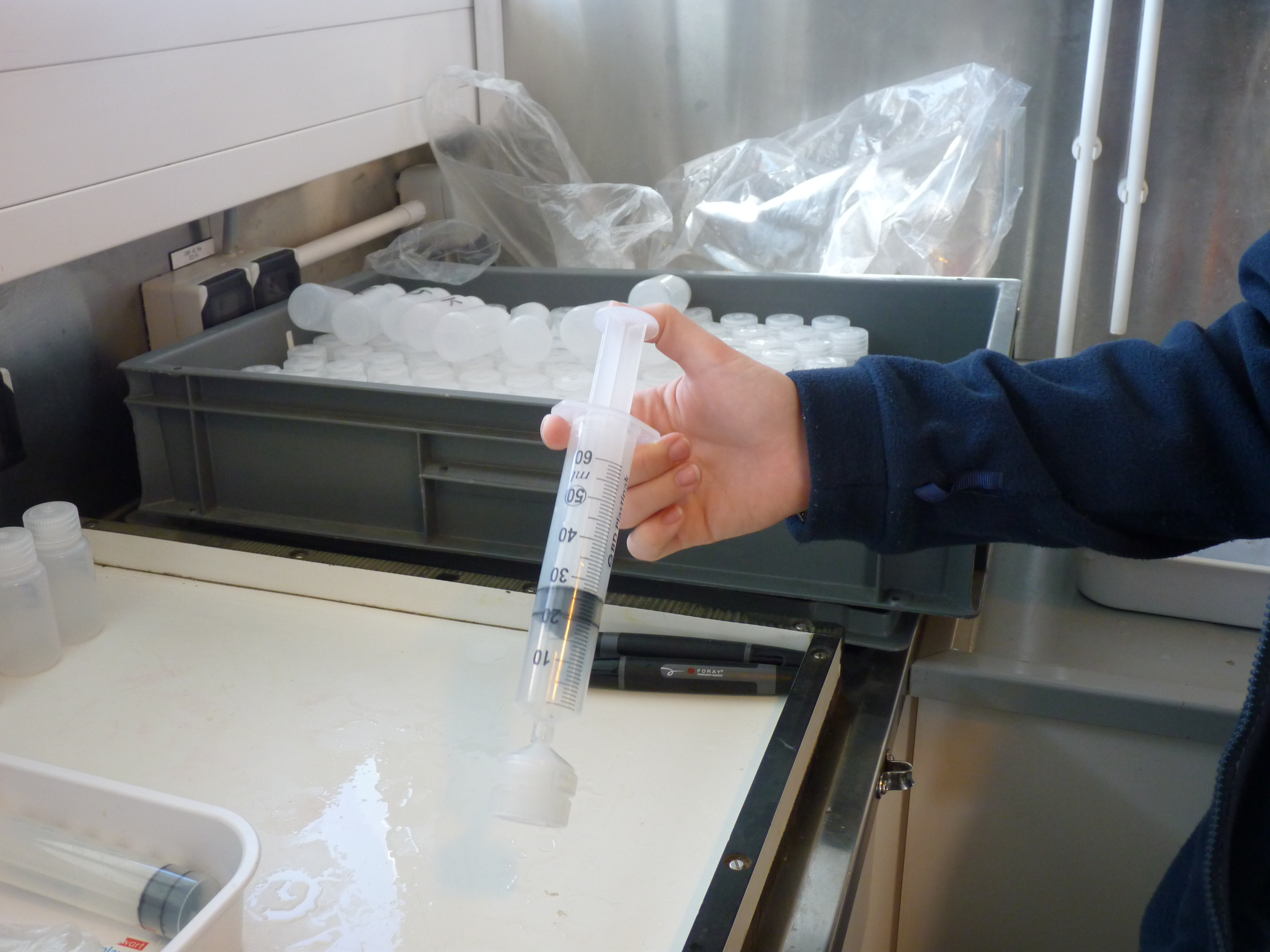
| Dissolved Oxygen | Once the CTD was recovered from the vertical profile, dissolved oxygen samples were decanted from a Niskin bottle to a glass vial. Care was taken to ensure that the vial overflowed to eliminate any air bubbles within the sample. 1ml of Winkler reagents (manganese chloride and alkaline iodide) (Winkler, 1888) were then added to each sample, shaken and stored in a temperature controlled container. |
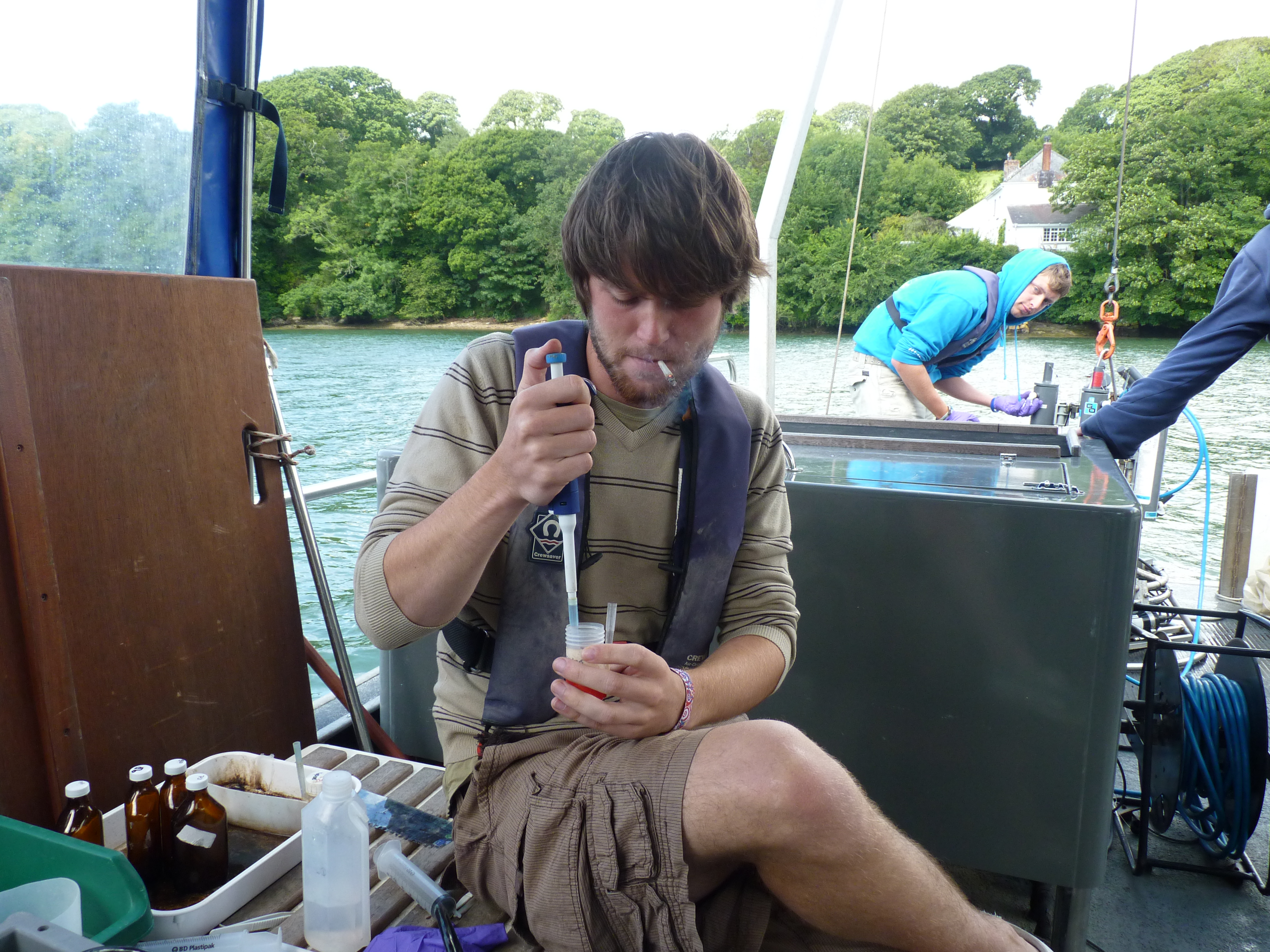 |
| Phosphate |
The water samples were collected from the Niskin bottles from the CTD cast by a plastic tube draining the water into a rinsed plastic container. A volume of 100ml from the water bottles was placed into brown glass bottles and placed into cold storage to preserve the sample until laboratory analysis. |
 |
| Phytoplankton | 100ml of seawater from the plastic container was siphoned off and 1 ml of Lugols iodine was added to it before storage in brown glass bottles. | |
| Zooplankton | Zooplankton were collected using a 200µm mesh and 0.6m diameter plankton net trawled vertically through the water column on Callista. The nets were closed using messengers to collect species for analysis from a specific depth range. On Conway the nets were trawled horizontally along a transect for 5 minute intervals, using a flow meter to calculate the volume of water being trawled. The samples were placed into sample bottles and formalin was added to preserve the sample. |
 |
| Chlorophyll |
50ml of raw seawater was filtered through a glass fibre filter. The filter paper was then put in a plastic vial containing 6ml of 90% acetone and stored in the fridge. |
 |
| Silicon | The 50ml of filtered water produced in chlorophyll preparation was decanted into a plastic bottle for laboratory silicon analysis. | |
| Sidescan collection & Ground truthing |
The sidescan sonar towfish was towed at a constant speed of four knots on a 2.5m cable behind the Grey bear vessel within the top 1m of the water column. We carried out four parallel 1300m transects and one 600m transect north of the previous four. The sonar frequency was low resolution (110 kHz) but the first four transects had high spatial resolution with 50m between each transect. Ground truthing was done by the use of a Van Veen Grab, where flora and fauna caught was identified and sediment grain size estimated.
|
 |
| Cloud Cover- Okta units |
Okta units are a method of describing cloud cover. The sky is hypothetically divided into four sections, and then an estimate is made whether each section has half or full cloud cover. With the four sections combined, a value out of eight is recorded to describe the cloud cover at each station. Cloud cover is important when sampling, as it affects the amount of irradiance hitting the sea surface, and will hence affect the distribution of phytoplankton and depth of light penetration.
|
 |
| Land Based Laboratory Methods of Analysis | ||
| Zooplankton |
The samples taken and preserved on the boat were taken to the lab where samples were mixed and 10ml placed in a measuring cylinder. This was then transferred, using a pipette, into a Borgorov chamber 5 ml at a time until 10ml had been processed. The Borgorov chamber containing the zooplankton sample was studied under a light microscope and the classes of zooplankton were identified and counted. |
 |
| Phytoplankton | The Lugols treated plankton samples were transferred into settling tubes to allow the phytoplankton to sink to the bottom and 90% of the solution was removed by a vacuum pump and u-bend tube system to concentrate the samples. Each sample was transferred to a 2ml Sedgewick-Rafter chamber and observed under a 400x magnified microscope lens. Five columns were viewed and the phytoplankton observed in these columns were counted and identified. The final count was then multiplied by 10 to give the total count in the chamber.
|
 |
| Silicon |
The silicate concentration for the filtered seawater samples was calculated by calibrating spectrophotometer readings of the samples after mixing with a reagent against readings from standards of known concentrations. Stock Si solution of 35.6 mmol/l was diluted 10 times for the estuarine samples (working standard A), and diluted 25 times to make up a working standard for the offshore samples (working standard B). 10, 25, 50, 75 and 100µl of stock solution were added to 5ml of MQ water. These then gave working standard A values of 7.1, 17.8, 35.6, 53.4 and 71.1 µmol/L, and working standard B values of 2.8, 7.1, 14.2, 21.4 and 28.5 µmol/L. Triplicated blanks (MQ water only) were also included. 5ml of the filtered seawater sample was added to each empty 13ml tube with a 5ml hand pipette. Replicates were taken of 1 sample in every 5, randomly selected. 2ml of ammonium molybdate reagent was added to each tube. The tubes were shaken and left to stand for 10 minutes. After the 10 minute standing period 3ml of the Mixed Reducing Agent was added to all of the samples, standards and blanks. The contents were mixed and the tubes were left to stand for 2 hours. The Mixed reducing agent was made from Metol sulphite, Oxalic acid, sulphuric acid (50% v/v) and MQ water in a ratio of 10:6:6:8. The absorbance of the samples, standards and blanks were measured using a U-1800 spectrophotometer set at 810 nm, and a 40mm cell. |
|
| Phosphate |
10ml from each sample taken and preserved on boat was place in individual sampling tubes, with 3 replicates randomly selected. Standards were made up by diluting a known concentration of phosphate to concentrations of 0.07µmol/l, 0.15µmol/l, 0.3µmol/l, 0.75µmol/l and 1.5µmol/l as well as including blank standards which were formed of milli-Q water. A mixed reagent was then made in a 2:5:2:1 ratio of ammonium molybdate, sulphuric acid, ascorbic acid and potassium antimonyl tartrate and 1 ml was added to each sampling tube and each standard. These were then left for 1 hour for the colour to develop. A U-1800 spectrophotometer measuring at 882nm using a 40mm cell was used to calculate the phosphate concentration of the samples. Each sample was poured into the cell and the spectrophotometer gave a reading. The concentration of the standards was plotted against the reading obtained by the standards to give a calibration curve used to convert the spectrophotometer readings into concentrations in µmol/l. |
|
| Dissolved Oxygen |
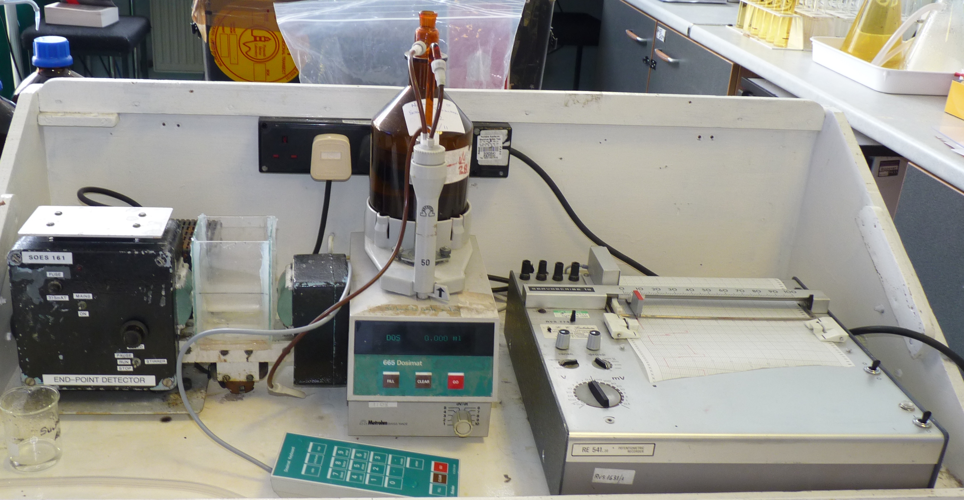
The samples had been collected and fixed in situ using winkler reagents. 1ml of sulphuric acid was added to re-dissolve the precipitate. Then the samples were then titrated in the lab against the neutralizing compound, sodium thiosulphate, which results in a colour change from yellow to colourless. The volume of sodium thiosulphate (normality of 0.22) added with an auto-burette used to reach this “endpoint” colour change relates stoichiometrically to the concentration of dissolved oxygen in the sample (Strickland and Parsons 1968).
|
 |
| Chlorophyll |
The filters prepared on the boats were placed in a freezer overnight to break open the cell membranes meaning that a sonication stage was not necessary. This lessened the risk of free radical generation which can react with the molecules and alter their chemical composition. The acetone-chlorophyll solution was then poured into a cuvette and allowed to settle before being placed into a fluorometer, which gave a measure of chlorophyll concentration (µg/L). The concentration may be corrected using the equation:
|
 |
| Offshore | |||||||||||||||||||||||||||||||||||||||||||||
|
Introduction |
|
||||||||||||||||||||||||||||||||||||||||||||
|
Offshore boat work was carried out on Callista on 30/06/2011. The aim of the offshore study was to look at differences in stratification and plankton distribution around a front, contrasting the differences between the more well mixed coastal waters and thermally stratified open shelf waters.
Five full stations, where a CTD profile, ADCP transect and water samples for analysis of phosphate, silicate, chlorophyll, phytoplankton and dissolved oxygen were taken at depths of interest, namely below, at and above the thermocline as indicated by the CTD readings. From the phytoplankton and zooplankton samples, species composition and
abundance could be investigated.
Using initial data from the CTD and ADCP, depths of interest were trawled vertically using a 200micron plankton net to get zooplankton samples. The water samples were later analysed in the laboratory.
Between each of the full stations a CTD was deployed so that the structure of the water column could be assessed. The vertical distributions of temperature and salinity, as well as the ongoing monitoring of the ADCP backscatter data was used to judge the presence of the front which was to be studied. The ADCP ran constantly but was used most effectively between stations 4 and 5 where the speed of the vessel was reduced to 4 knots.
The light meter was malfunctioning and strong currents meant that the secchi disk data is unreliable and therefore light attenuation data cannot be utilised in our evaluations. |
|||||||||||||||||||||||||||||||||||||||||||||
| Results & Discussion | |||||||||||||||||||||||||||||||||||||||||||||
|
Nutrients: Phytoplankton require both light and nutrients to grow. The nutrients available to the phytoplankton are partially dictated by the extent of water column mixing. In areas where phytoplankton is abundant, nutrient levels become depleted if there is not sufficient mixing bringing up nutrient rich waters from depth. Phosphate is one of the essential nutrients required by all phytoplankton groups. However, phosphate is not needed in huge concentrations, and is therefore not usually the limiting factor upon phytoplankton growth. Dissolved silica is utilised by diatoms to construct their silica frustule: Therefore, in areas where diatoms dominate, dissolved silica often becomes quickly depleted after the spring bloom and can limit diatom growth, resulting in succession during the summer months in temperate regions to different phytoplankton groups, predominantly dinoflagellates (Widdicombe et al. 2010). Nitrate is also an essential nutrient required universally for phytoplankton species, however, nitrate levels were not analysed on the offshore boat practical. The water samples collected on board the Callista were analysed in the laboratory for dissolved nutrients, using methods detailed in the Laboratory Methods section. At station 1, the depths water samples were taken were very shallow (surface, 4.2m, 8m) as this station was well mixed and the largest temperature change, caused by surface heating, was in the top 4m of the water column. Throughout the 30m deep water column sampled using the CTD there was less than 0.6°C temperature change. Laboratory data shows a chlorophyll peak at 4.2 m of 2.91µg/l (see figure 1), which corresponds to a lower value of dissolved silica at this depth of 1.75µM (see figure 2). This suggests the presence of diatoms, supported by the phytoplankton analysis where the marine diatom species Thalassiosira nordenskioeldii was the dominant type in the Lugol’s iodine preserved phytoplankton sample (see figure 3). The phosphate data for station 1 shows a decrease in phosphate concentrations with depth for the depths sampled, dropping from around 38µmol/l to under 20µmol/l in the top 8m of water. Station 1 was the only well mixed station sampled, having been on the inland side of the thermal front. Station 2 (figure 4) shows a lower concentration of dissolved silica at 32m than 5m depth. The chlorophyll data for these depths shows an opposite pattern. This suggests that the silica was being taken up by the increasing phytoplankton numbers. The phytoplankton data shows that at each depth, diatom species were the most abundant, with the 5.1m depth sample dominated by Thalassiosira constricta, the 17.5m sample dominated by Cerataulina pelagica and the 32m sample by Guinardia striata. The phosphate concentration was lowest at and above the thermocline, and higher below it. This shows that there was a high enough phosphate concentration to support increasing phytoplankton numbers. At station 3 (figure 5) silica increased with each depth sampled down to 32m. The chlorophyll concentration decreased with depths sampled to 19m then increased towards 32m, supported by the CTD flourometer voltage reading which indicates a relative chlorophyll maximum at around 35m. The phosphate decreases in concentration down to 19m then remains at a very low level (close to 0µmol/l) down to 32m. This suggests that the increased chlorophyll concentration, indicating an increased number of phytoplankton cells, used up the phosphate at this depth. At stations 4 (figure 7) and 5 (figure 5a) the silica concentration generally increases with depth, although there is a decrease in silica concentration at station 4 at a depth of around 18m. The chlorophyll data for station 5 shows a maximum at 18m and the phytoplankton data show that the dominant species were diatoms, which could account for the decreased silica value. The phosphate concentrations at stations 4 and 5 decreased with depth, although a maximum was observed at 18m for the phosphate at station 5. The phosphate values, as expected, generally decreased with depth, as it was utilised by the phytoplankton. However, there were some exceptions to this trend; a possible reason for this is that the phosphate samples were not filtered on the boat. As a result of this some phosphate uptake by phytoplankton could have occurred whilst the samples were stored prior to laboratory analysis. Silica distributions were also as expected. Where diatoms dominated the phytoplankton, silica levels decreased indicating utilisation by the diatoms. Concentrations of phosphate and silicate were only measured at 3 discrete depths at each station, so any inference of trends from the data is difficult as the intermediate concentrations are unknown.
|
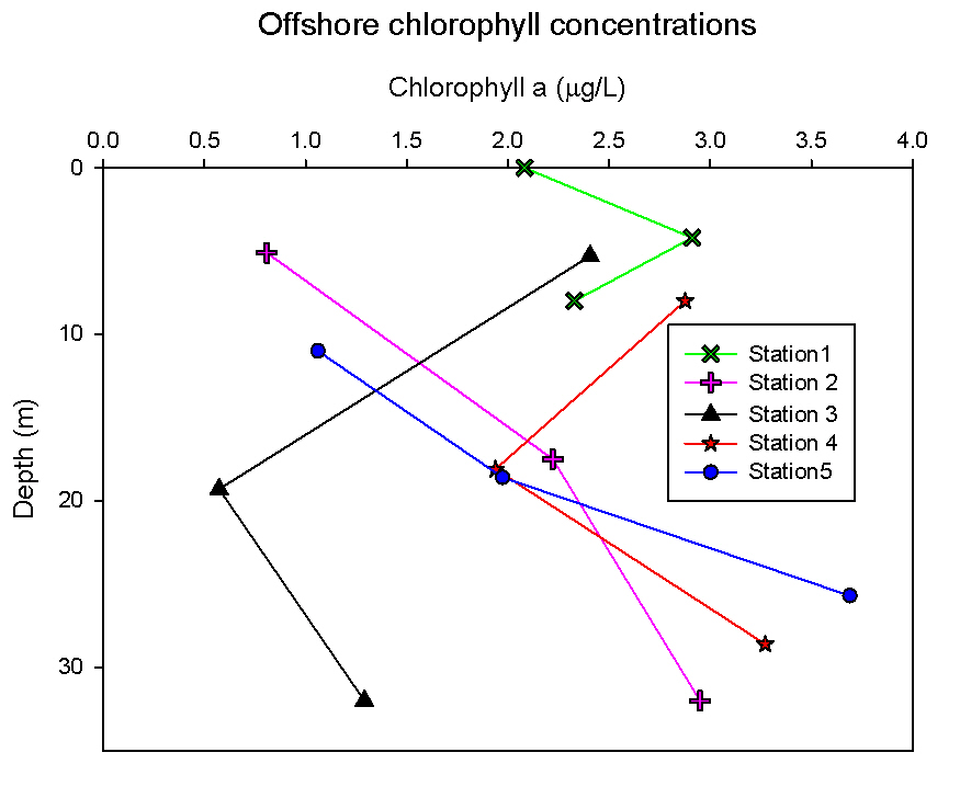
figure 1: Offshore chlorophyll concentration depth profiles for all stations.
figure 2: Station 1 CTD & nutrient depth profile
figure 3: Offshore phytoplankton species abundance and identification
figure 4: Station 2 CTD & nutrient depth profile
figure 5- Station 3 CTD & nutrient depth profile.
figure 5a- Station 5 CTD & nutrient depth profile. |
||||||||||||||||||||||||||||||||||||||||||||
| Dissolved Oxygen: When a body of seawater is fully saturated with oxygen, it is described as 100% saturated. If the seawater has a dissolved oxygen value of above 100% it is described as super-saturated, and in contrast, if below 100% the seawater is under-saturated. Any values which fall above 100% indicate an active input of oxygen to the environment, for example a high number of phytoplankton cells photosynthesising and releasing oxygen. Any number falling below 100% indicates that oxygen is being removed from the environment, for example a number of zooplankton exceeding phytoplankton and respiring, taking up oxygen. At station 1 the oxygen saturation is 259% at the surface, and this falls to 98.4% at 4m and 97.8% at 8m (see figure 6). The very high value for the surface sample could be a result of movement of oxygen at the water-air interface, with oxygen diffusing into the surface layer or being entrained by any choppiness. There is a decrease in both dissolved oxygen percentage and chlorophyll concentration are higher at 4m than 8m depth. Using chlorophyll as an indicator for phytoplankton, this suggests that the decreased photosynthesis, attributed to decreased phytoplankton resulted in a decrease of oxygen input to the surrounding water. The oxygen saturation at station 2 at 5m is 233.6%. At 17 m the saturation is 109.6% and then is higher at 32m with a percentage saturation of 111.5% (see figure 6). At station 3 the oxygen saturation at 5m is 100%. At 19m it rises to 106% and then falls to 89.8% at 32m. At station 4 at a depth of 8m the oxygen saturation is 103%. At 18m is rises to 125.3% then falls to 84% at 28m. The oxygen saturation at station 5 at 11m is 114.1%. This drops to 87.6% at 18m then rises slightly to 90.5% at 25m. To conclude, there is a general pattern of decreasing dissolved oxygen concentration with the depths sampled. However, stations 3 and 4 showed higher values of dissolved oxygen at mid depths, both at around 20m. At these stations, 20m was the base of the thermocline (see figures 5 and 7). These figures also show a fluorometer reading maximum below the base of the thermocline, indicating increased chlorophyll thus supporting this finding, as the phytoplankton associated with increased chlorophyll will increase the percentage saturation through increased photosynthesis. As the dissolved saturations were calculated only at 3 discrete depths per station, more detailed patterns than those observed were present.
|
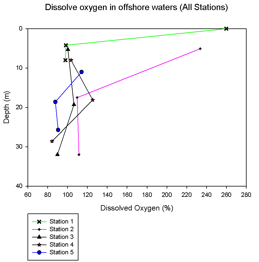
figure 6: Offshore Oxygen concentration depth profiles for all stations.
figure 7: Station 4 CTD and nutrient depth profiles. |
||||||||||||||||||||||||||||||||||||||||||||
|
Zooplankton The zooplankton data were graphed showing the variations in zooplankton composition at each station, showing variations in total zooplankton numbers as well as changes in composition between zooplankton groups. The numbers were calculated as a concentration to make data from different stations, where different volumes of water were sampled, comparable. At station 2, two plankton trawls were taken: 2b is from 30-15m and 2a is from 12m to the surface. Closer to the surface siphonophorae are the most abundant zooplankton whereas at depth copepods were most abundant (see figure 8). This can be explained by the fact that copepod numbers are dominant at the thermocline as they can maintain their position in the water column and their position in the water column is typically controlled by the hydrodynamic characteristics of the water column (Rodriguez et al, 2000). This shows that there is not only a variation of the zooplankton numbers at different depths but also a variation in their composition at this station. The greatest numbers of zooplankton were at station 5 where the depth of the thermocline was greatest and high numbers of phytoplankton were found at the depth of sampling. At station 3, 4 and 5 the dominant type of zooplankton were not copepods but hydromedusae; this can be partially explained by the fact that the dominant zooplankton type may be controlled by the sea surface temperature (Hawkins et al, 2003). At stations 3 and 4 the sea surface temperature was above 14.5°C compared to around 13.6°C at station 1, which could explain some of the change in these stations. Copepods are inhibited by the quality of food and the existence of G. aureolum in the water column (Harris, 1988) which could give rise to a dominance of hydromedusae. An increase in numbers of hydromedusae in the water column could be caused by the predation of these on copepods (Hirst, 2007). At these stations the types of phytoplankton were different to those found at stations 1 and 2, which are located further west. This could be due to differences in the strength of the thermocline which is strongest at station 3, 4 and 5. |
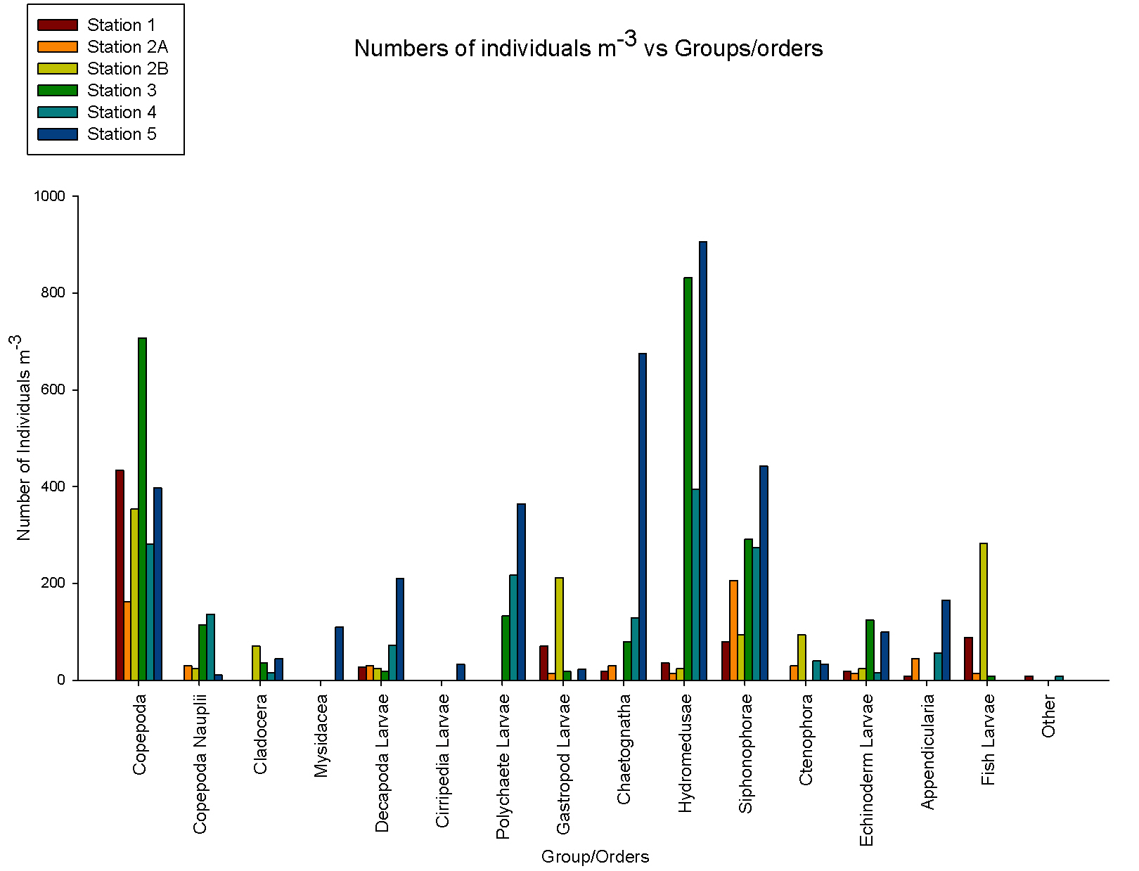
figure 8: zooplankton species & abundance at all offshore stations.
|
||||||||||||||||||||||||||||||||||||||||||||
|
Phytoplankton The changes in numbers of phytoplankton from three groups - diatoms, dinoflagellates and ciliates – were examined against depth in order to complement data showing the change in phytoplankton species across different stations and depths. This allows trends to be identified at the different stations and can give information relating to nutrient distributions. There is a continuous trend at all 5 stations with respect to total diatom numbers with total numbers increasing with depth (see figures 9,10,11,12,13). At all stations the dominant phytoplankton group was diatoms. At stations 1 and 2, Cerataulina pelagica and Guinardia striata were the dominant species (see figure 3). At stations 2 and 5 Thalassiosira constructa replaced C. pelagica but G. striata was still abundant. Station 4 Chaetoceros compressus and Thalassiosira angulate were dominant. There are differences in the dinoflagellate numbers between the more coastal stations (1, 2 and 5) and the more offshore stations. In the three more coastal stations dinoflagellate numbers are highest at the surface and non-existent at depth. This varies from 2 dinoflagellates ml-1 at station 1to 0.5 dinoflagellates ml-1 at station 2 and 12.5 dinoflagellates ml-1 at station 5. All of these stations have 0 dinoflagellates ml-1 at depth. At stations 3 and 4 this trend is mirrored with highest dinoflagellate numbers at depths of 32m and 28m respectively. At station 3 there are 7 dinoflagellates ml-1 and at station 4 there are 8.5 dinoflagellates ml-1. Ciliates vary greatly amongst the stations. There were no ciliates found in stations 1 and 2 but were found at station 3 at a depth of 32m, station 4 at around 18m and station 5 close to the surface. The most abundant dinoflagellate species, found at stations 3 and 4, was Dipslosalis lenticula. Karenia mikimotoi was a dinoflagellate found uniformly in low numbers across all stations sampled. This variation in the types of phytoplankton and where dinoflagellates were found can be used as an indicator of the location of a front. Dinoflagellates are controlled by where the front is and in midsummer exist in stratified waters at the thermocline, which explains their distribution in offshore waters. The dinoflagellate numbers at the more coastal stations are greater at the surface due to the effect of tidal mixing which brings nutrients to the surface. Since the tidal effect is greater at coastal stations this controls dinoflagellate numbers here whereas the thermocline explains dinoflagellate numbers at the more offshore stations (Holligan and Harbour, 1977). Total numbers of phytoplankton are seen to increase at all stations with depth. This relates to the depth of the thermocline where there is the highest abundance of nutrients as nutrients are quickly used up above the thermocline but recycled below it. |
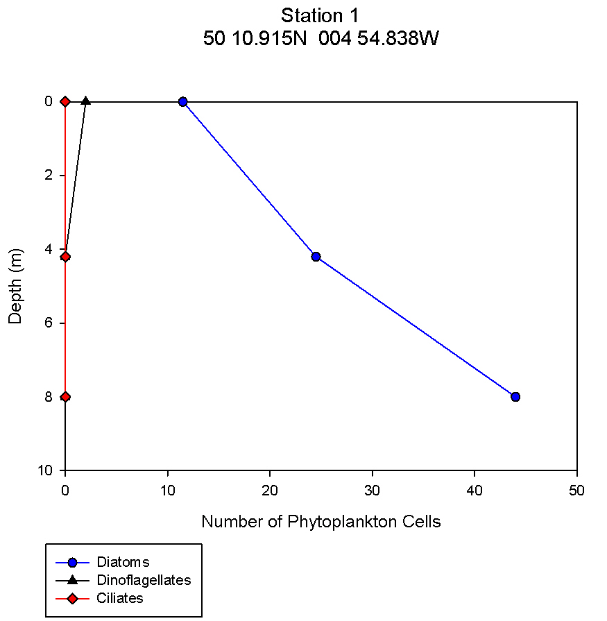
figure 9: Station 1 phytoplankton abundance depth profile.
figure 10: Station 2 phytoplankton abundance depth profile.
figure 11: Station 3 phytoplankton abundance depth profile.
figure 12: Station 4 phytoplankton abundance depth profile.
figure 13: Station 5 phytoplankton abundance depth profile.
|
||||||||||||||||||||||||||||||||||||||||||||
|
ADCP ADCP Transects Transect 1 was taken at Blackrock (50.08.660N 005.01.461W) at 7:57GMT in the middle of high and low water. The average flow direction was 152.34 degrees South south East in the upper part of the water column and was 220.21 degrees at the water sea floor boundary. The average velocity magnitude was 0.231m/s in the upper part of the water column comprising the top 15m in the deeper portion of the plot, where the deeper areas (the bottom 15m) had a lower average velocity of 0.051m/s (see figure 22). The backscatter received was concentrated from 5 to 10m with an average reading of 79dB. The backscatter indicated a high amount of mixing with signals being bounced back throughout the water column (see figure 23). This high average backscatter could be due to mixing of nutrients into the upper column of nutrient depleted water allowing greater plankton growth near the sea surface. Transect 2 was taken at Station 2 (50.01.898N 005.00.954W) at 9:30GMT, data for velocity and backscatter was interrupted by Callista engine bursts. The maximum backscatter was from 17m which showed an average of 80dB with a second line of backscatter seen at 32m with a value of 74dB. The velocity had increased from station 1 to with an average of 0.632m/s down to 35m below which the value fell to 0.402m/s. The velocity direction was South West on an average bearing of 210.20 degrees. This direction change from stations 1 to 2 corresponds with the ebb flow from the English Channel. Transect 3 was taken at station 3 (50.05.025N 004.54.862W) at 11:29GMT, 47 minutes after high water. The maximum backscatter was seen at 19m with an average of 78dB and a second line of backscatter was seen at 25m with an average value of 75dB. The velocity magnitude was 0.412m/s down to 20m and then dropped to 0.110m/s down to the sea floor. The velocity direction also changed with depth starting at an average of 230 degrees and changing to a mainly Westerly flow with a 268 degree average. Transect 4 was taken at station 4 (50.07.740N 004.49.010W) at 13:04GMT, with results of ADCP showing very little data was collected due to Callista engine interference . The average backscatter when visible showed two parallel lines of strong readings with the first occurring at 15m and the second at 25m. The shallower bar gave higher average backscatter results of 78dB compared to that of 75dB at 25m. There is evidence of some internal wave action resulting from gravity waves oscillating within the water column. These waves may be the result of river plumes from the Fal estuary as Nash and Moum (2005) have shown that internal waves can be generated by river plumes flowing as a gravity current into the open ocean. These can be seen in the backscatter readings causing the main lines of reflection within the water column to show peaks and troughs. The average velocity magnitude of the transect is 0.14m/s and due to poor quality readings along this transect it is not possible to discern the velocity direction. Transect 5 was taken at station 5 (50.10.672N 004.53.424W) at 14:44GMT, the greatest average backscatter recorded was between 7m and 25m. Two lines of high backscatter could be seen occurring at 8m and 15m both returning an average value of 79dB (see figure 24). The velocity magnitude remained constant throughout the water column at 0.125m/s (see figure 25) and the velocity direction showed a North East flow, 55.36 degrees, with increased activity and change below 13m. The readings indicate a greater degree of directional change and shear within the water column when compared to the previous transects. This may suggest the emergence of a front in the area that would appear in shallower conditions. The ADCP data for velocity and CTD data for density were used to calculate the Richardson’s number. The Richardson Number (Ri) is a dimensionless ratio between the change in density and velocity shear (magnitude and direction) with depth and can be calculated using the following equation (Knauss,1997):
Where g is gravity, ρ is density, dρ is the change in density, and du is change in velocity. The water column was divided into 1m layers for Station 1, and 5m layers for the deeper stations, in order to calculate the change in density and velocity. When Ri is small, below 0.25, then velocity shear will be of sufficient strength to overcome the stratification of a body of water and cause mixing to occur (Turner, 1973). Values falling between 0.25 and 1 show shear instability where mixing will continue at a lesser degree and values above 1 indicate a stable flow. Station 1 was taken at Blackrock with CTD values recording down to 27m which showed a mixed profile with low Ri values throughout the water column (see figure 14). Values at depths of 7m, 18m and 20m showed stable flow with the highest mixing values coming in the bottom 5m of the profile from 22m to 27m with an average value of 0.0494 indicating gravitational instability. Station 2 recorded CTD down to a depth of 60m. The Ri values indicated mixing occurred within the top 20m (average of 0.307) with a high Ri value occurring at 20m (15.368) signifying the start of the thermocline (see figure 15). The Ri values below 20m were all above 13.884. Station 3 recorded CTD data down to a depth of 55m. Ri values observed down to 20m were below 1 (average of 0.7258) suggesting mixing occurring in the upper layer of the water column (see figure 16). At 20m and below the values increased to above 1 with the highest occurring from 35m-40m (19.627 and 14.138 respectively) indicating a stable layer. Station 4 recorded CTD data to a depth of 56m. Ri values (see figure 17) calculated to 25m indicated mixing by shear instability with values falling between 0.25 and 1 (average of 0.538). Ri values, between 25m to 35m and 45m to 55m, were above 1 (average 3.697) signifying a stable flow at these depths. The Ri values observed at 35m, 40m and 55m all indicated unstable flow with the values at 35m and 40m were under 0.25 (0.0213 and 0.0481) therefore gravitational instability was assumed. Station 5 recorded CTD data to a depth of 29m. Ri values (see figure 18) observed to a depth of 15m indicated shear instability causing mixing with values <1 and >0.25 (average 0.911). Ri calculated values from 15m to 25m (average of 1.766) suggested stable flow and below this unstable shear and gravitational flow was observed 0.468 and 0.069 at depths 25m and 29m respectively. Coastal waters are generally areas of well mixed water due to low water column depths and increased tidal mixing. Moving offshore the profile of the water column will change due to alterations in the proportions of the forces acting upon it, the expected changes will be an increase in wind stress and a decrease in tidal mixing. The decrease in tidal mixing will be far greater proportionally when compared to the increase in wind shear which will lead to stratification. Due to the decrease in tidal mixing stratification can also be developed by solar heating. The shelf sea in Falmouth can be divided into seasonally stratified and mixed regions. The mixed regions are indicated by colder surface temperatures, seen on the CTD. At the frontier between these regions, which is known as a tidal mixing front (Simpson and Hunter, 1974), the change can also be seen on ADCP data as a front is accompanied by a sharp change in velocity. At station 1 the water column was well mixed (see figure 19) with the temperature remaining within a range of 0.5°C throughout the depth sampled. Stations 2, 3, 4 and 5are stratified by temperature showing clear thermoclines in the water column (see figure 20, 5, 7, 21). This is supported by the Richardson’s number calculations which show turbulent mixing throughout depths (see figure 14). At station 2 it is at a depth of 10m (see figure 20) and there is a second further thermocline at 13m. This second thermocline could be a result of downward mixing, supported by the Richardson’s number calculations which show turbulent mixing above about 11m (see figure 15). At station 3 the temperature drops from 14.5°C to 12°C with a steep thermocline at 15m (see figure 5). At station 4 a similar pattern is seen to station 2 with a second section of the thermocline appearing to be mixed downwards (see figure 7). Station 5 shows a temperature change of around 1.5°C between 14m and 17m which is again supported by the observed Ri values indicating stable flow from 15m to 20m. |
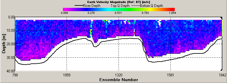
figure 22: ADCP velocity magnitude plot from mixed station.
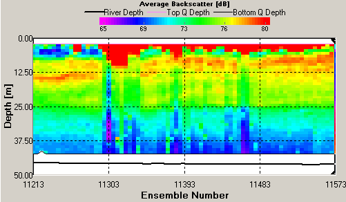
figure 23: ADCP backscatter plot from mixed station
figure 24: ADCP backscatter plot from stratified station.
figure 25: ADCP velocity magnitude plot from stratified station
figure 14: Station 1 Richardson number depth profile.
figure 15: Station 2 Richardson number depth profile.
figure 16: Station 3 Richardson number depth profile.
figure 17: Station 4 Richardson number depth profile.
figure 18: Station 5 Richardson number depth profile.
figure 19: Station 1 CTD depth profile
figure 20: Station 2 CTD depth profile
figure 21: Station 5 CTD depth profile |
||||||||||||||||||||||||||||||||||||||||||||
| Conclusion | |||||||||||||||||||||||||||||||||||||||||||||
|
Several clear patterns emerged from the offshore data: Diatoms were the dominant phytoplankton at all stations, and their abundance had an inverse correlation with dissolved silica concentrations. Silica was at its highest levels at deeper waters, below the thermoclines, where it is not being utilised by the diatoms. Chlorophyll generally had an intermediate peak, and then decreased above and below this depth. Phosphate appeared to decrease with depth at all the stations, indicating its utilisation by all phytoplankton groups. Dissolved oxygen concentrations mostly decreased with depth, although stations three and four had an intermediate maximum at the base of the thermocline. Zooplankton distribution had less of an obvious pattern; copepods tend to dominate the thermocline, whereas hydromedusae dominated the offshore stations. Richardson’s numbers and ADCP data were used to distinguish between the well mixed turbulent stations and the stratified offshore stations. Station one was the only well mixed station sampled and was on the landward side of the thermal front whereas stations two to five had obvious thermoclines and patterns of nutrients, dissolved oxygen, and showed different characteristics of flow and stratification. Data for the estuarine mixing diagram used salinities collected using a YSI30 probe (number F202). A calibration was applied to the data collected to ensure accuracy. No changes were made as the YSI30 measured temperature and salinity to one decimal place, and at this level of accuracy the calibrated values were identical.
|
|||||||||||||||||||||||||||||||||||||||||||||
| Geophysics | |||||||||||||||||||||||||||||||||||||
| Introduction |
|
||||||||||||||||||||||||||||||||||||
|
St. Mawes is located on the eastern side of the macrotidal Fal estuary, Cornwall UK. The Fal Estuary is a ria system which developed in response to Holocene sea-level rise (Bird, 1998).The estuary extends 18km inland from its mouth to its northern limit at Tresillian and has a total shore line of 127km (Pirrie et al., 2003).
The regional geology surrounding the estuary is mainly granite dominated (Leveridge et al., 1990). It is classified as a tide swept channel where the estuary acts as a funnelling system of seawater towards the coast. These tides can funnel nutrient rich waters into the estuary, meaning that there is opportunity for plentiful marine life. The Fal estuary has many conservation statuses protecting its biodiversity and ecosystem health.
At St. Mawes bay, there are extensive beds of calcareous red seaweed called maerl. There are also extensive meadows of eelgrass within in the estuary, which too, have warranted environmental protection. Maerl is slow growing and grows as rhodoliths, brittle pink nodules. The maerl is not attached to the seabed, which makes it even more susceptible to anthropogenic practices. These extensive seabeds provide a habitat for a wide range of phyla, including molluscs, anemones, worms and decapods crustaceans.
Bids to dredge the Fal estuary to accommodate larger shipping vessels have been declined due to the high biological status of the maerl beds: Dredging and increased shipping and hence changes in hydrographic conditions and an increase in anchoring are thought to have significant detrimental effects on the maerl beds.
Sidescan sonar is a geophysical marine technique that uses pulsed sonar to determine water column depth and the bathymetry, sediment characteristics, bedforms and even anthropogenic features such as anchor and dredge marks on the seafloor. The strength and return time of the sonar pulses allows these different features and characteristics to be analyzed.
The estuarine area around St. Mawes bank was surveyed using sidescan and 3 grab samples on the 4th of July 2011. Dominant winds were from the south, with mostly no cloud cover and sunny conditions. Due to the weak winds, seawater surface was calm. |
|||||||||||||||||||||||||||||||||||||
| Maerl | |||||||||||||||||||||||||||||||||||||
| Over the last century, maerl has stood as a small scale income source for European economies. Traditionally, it was dredged for its use as a soil conditioner. In the 1970s, France processed 600,000 tonnes of maerl per annum for this use. In Contrast, in the Fal estuary between the years of 1975-1991 only 30,000 tonnes has been extracted. Despite comparatively low harvesting, the slow growth rate of the organism makes the maerl beds a very fragile, susceptible and non-sustainable resource. Maerl beds act as a unique biotope, harbouring many endemic species and act as juvenile fish nurseries and are mainly threatened by extensive commercial extraction, heavy demersal fishing gear and degrading water quality. Maerl beds are awarded their international conservation significance as they create areas of high biodiversity .Anthropogenic practices such as scallop dredging has been shown to reduce maerl biomass by >70% (Hall-Spencer&Moore, 2000). A reduction in maerl abundance can have a detrimental cascade effect on its associated benthos, e.g. Limaria hians. Maerl is now the subject of a Habitat Action Plan under the UK Biodiversity Action Plan and occur in three demonstration SACs within the UK while the Fal and Helford candidate SAC includes the largest maerl bed in England. (http://www.ukmarinesac.org.uk/communities/maerl/m1_1.htm)
|
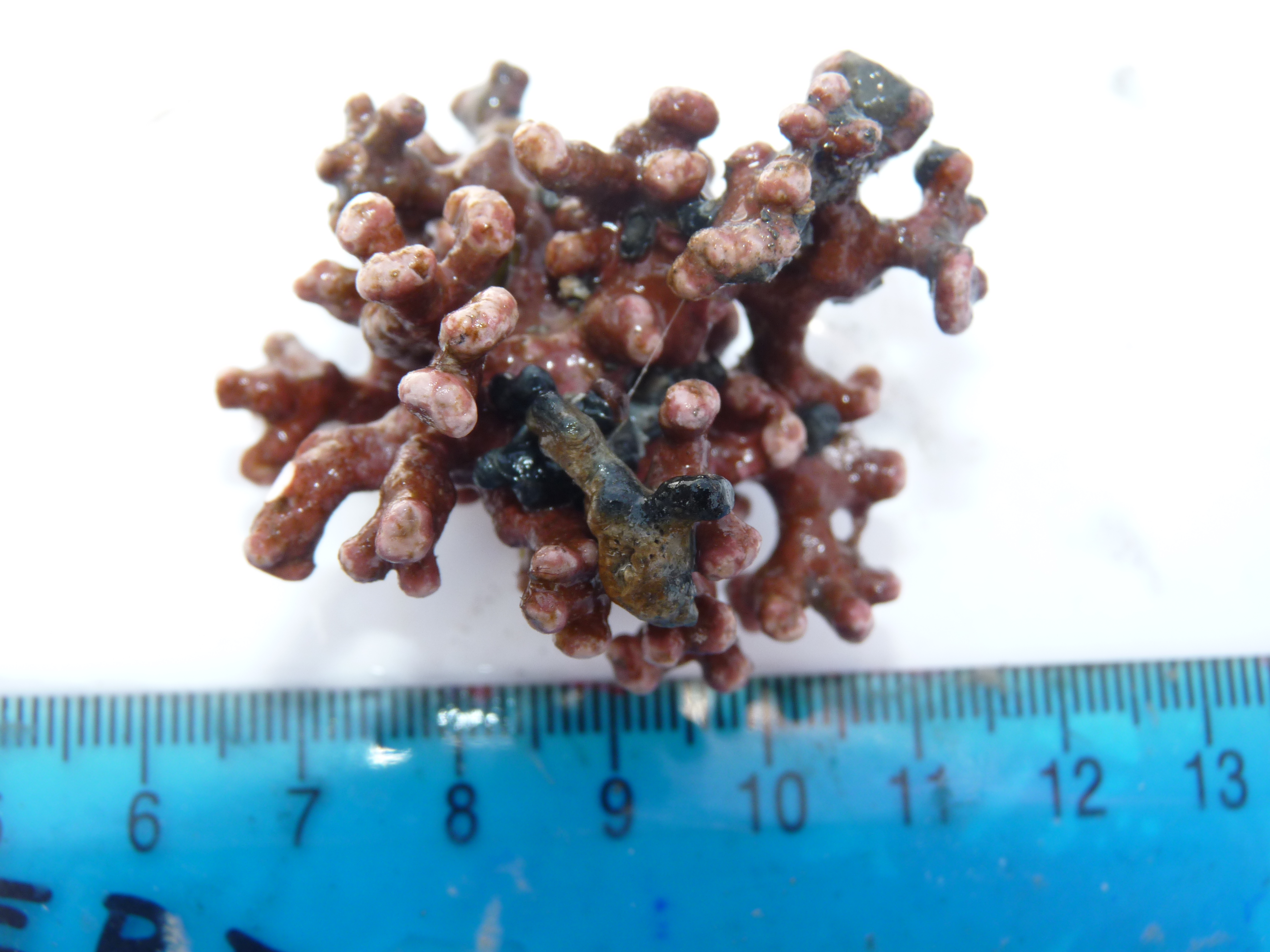
figure 22: maerl recovered from grab site 2. |
||||||||||||||||||||||||||||||||||||
| Grab Fauna | |||||||||||||||||||||||||||||||||||||
The main sediment type at grab-site 1 (figure 23) is silty clay, and fine sand with a covering of small (<5mm) shell pieces. The fauna present were bivalves and tubiculous polychates. Chlamys varia (figure 27) lives sublittorally down to 100m depth. It is usually found on rocky or firm sediments. Ostrea edulis (native oyster, figure 26) has a UK wide distribution, although it is mainly found in the Solent, the river Fal and west Scotland. It is associated with highly productive estuaries and shallow coastal habitats. It prefers firm bottoms of mud, rock or sand. Also found in the grab were various vagile and tubicolous polychates including Phyllochaetopterus anglicus. At grab site 2 (figure 24) the main sediment was fine silt and clay. 90% of the grab sample was made up of large (>40mm) clumps of pink maerl. Interspersed among the maerl on the seabed were patches of Calliblepharis cilrata. The fauna found in the grab sample included the crustaceans Galathea dispersa (squat lobster), Pisidia longicornis (porcelain crab) and carcinus maenas (shore crab). G. dispersa lives between 10 and 50m in the sublittoral zone, it has a European distribution from Norway in the north to Mediterranean in the South. Pisidia longicornis is a small (<10 mm) littoral crab with large claws with a distribution around the whole of the UK coastline. Carcinus maenus is the European shore crab that has a distribution around the whole of the continent, and has also invaded America and Oceania. It is euryhaline, and is able to tolerate salinities from 18-52%o. It can therefore live anywhere from the sea to the top of an estuary. The lugworm Arenicola marina was also found in the grab sample. At Grab site 3 (figure 25) the sediment that was found was predominantly clay, very fine sand and silt. This was accompanied by an abundance on young maerl, Sargassum and Himanthalia elongata as flora. In this part of the Fal estuary maerl is commonly found as there is a lack of wave action but a high water flow rate, providing the ideal conditions for maerl. The fact that the maerl is mainly young maerl can be attributed to an anthropogenic impact on the maerl in the estuary. At a depth of just over 10m there is sufficient light for healthy growth. Sargassum is not typically found in these areas as it usually grows on hard substrates and could have gotten into this grab by being washed along by strong bottom currents. Himanthalia elongata usually grows on hard substrates too and so again is uncommon to be found in this grab leading to the assumption that pieces of seaweed are washed off from harder substrates by strong bottom currents. The fauna found in this grab included the crustacean Carcinus maenas along with the molluscs Ensis arcuatus and Venerupis senegalensis the polychaetes Lanice conchilega, Nephtys caeca and Arenicola spp. Carcinus maenas is the common shore crab and can usually be found in shallow water estuarine habitats due to its ability to tolerate a wide variety of salinities and temperatures. This it is not uncommon to find it here. Both of the molluscs can commonly be found in the temperate estuarine environment but usually occur in a more sheltered environment and so may be a feature of the stronger bottom currents having washed them away. The polychaetes are more common to shallower sediments but not completely uncommon at a depth just over 10m. They are all tolerant to the stronger currents and the finer sediment types and so can be commonly found here.
|
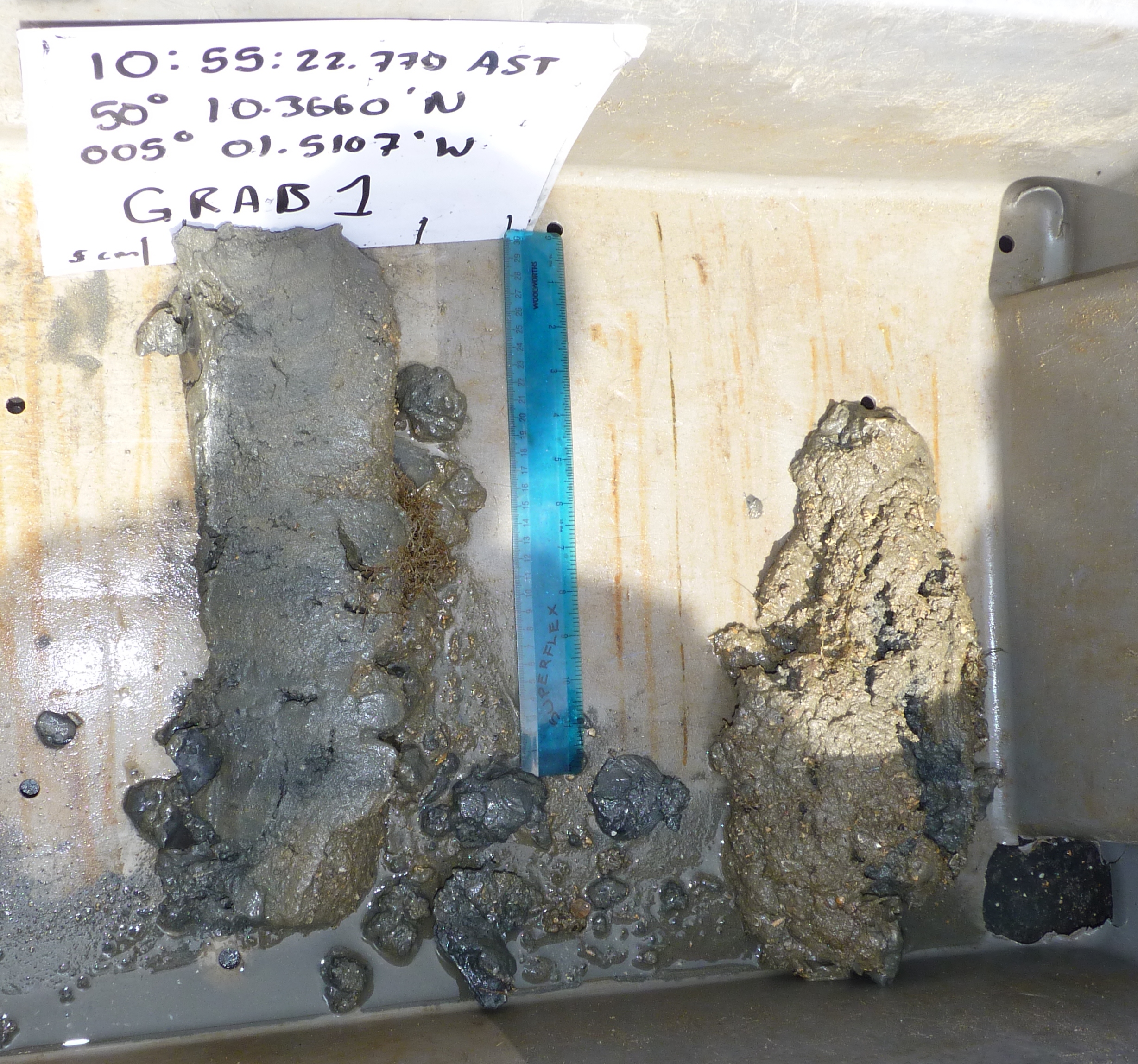
figure 23: Grab sample 1
figure 24: Grab sample 2
figure 25: Grab sample 3
figure 26: Ostrea edulis recovered from grab site 1.
figure 27: Clamys varia recovered from grab site 2.
|
||||||||||||||||||||||||||||||||||||
| Video Analysis of the seafloor at grab sites. | |||||||||||||||||||||||||||||||||||||
| In video recording 1 the dominant sediment type was a medium sandy bottom with empty bivalve shells. There are frequent patches of ulva lactuca. The observed fauna were Spiny Starfish (Marthasterias glacialis, figure 29),fanworms (Megalomma vesiculosum, figure 28), hermit crab (Paguras bernhardus) and shore crabs (Carcinus maenas). There was also an unidentified elasmobranch (probably a dog-fish, Squalus acanthius, figure 30) resting on the sea-bed.
At video site 2 the entire bottom was covered in maerl. This maerl ranged in size from ~3mm- >50mm. The maerl is inter-dispersed with patches of Dictyota dichotomy. The fauna included oysters (Ostrea edulis), along with 1 other unidentified bivalve. There were also snakelocks anemones (Anemonia viridis) and 2 spiny starfish (Marthasterias glacialis, figure 29).
The 3rd video recording showed a sandy bottom type with a covering of some immature maerl and some dead maerl. There was evidence of tubeworm burrows and razor clam shells. The dominant macroalgae was Rhodophyta. The invertebrate fauna consisted of snakelocks anemones (Anemonia viridis), sea squirt colonies (Ascidiella aspersa) and spiny starfish (Marthasterias glacialis, figure 29). There were also some adult and juvenile teleost fish.
|
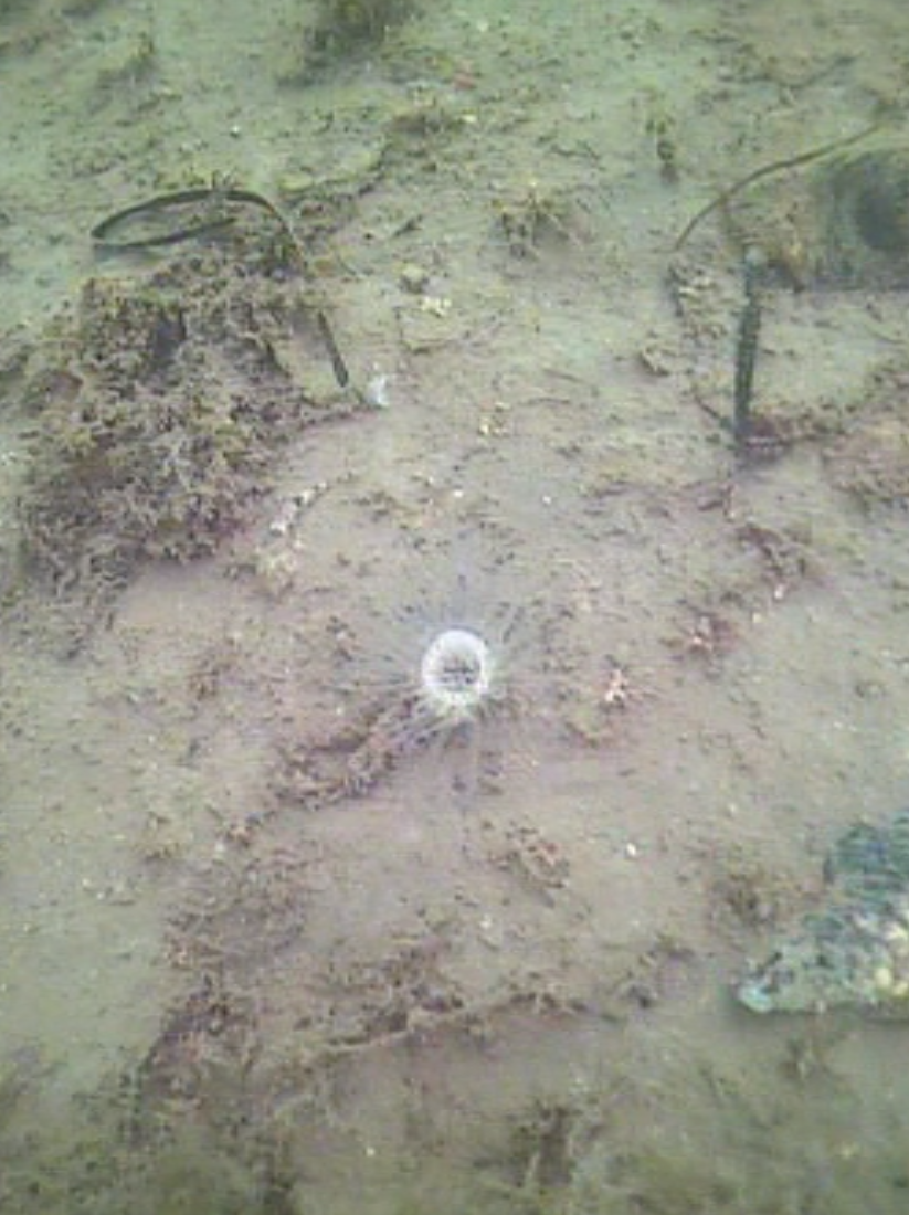
figure 28: Megalomma vesiculosum found in sea floor video at grab site 3.
figure 29: Marthasterias glacialis found in sea floor video at grab site 2
figure 30: possible Squalus acanthius found in sea floor video at grab site 1 |
||||||||||||||||||||||||||||||||||||
| Results and Discussion: | |||||||||||||||||||||||||||||||||||||
|
Transects 1 to 4 run from East narrows towards Shag rock (see figure 31): This ran into the channel towards the end of the 4 transects. Deeper water was the reason for fine sand at the time-tag of 08:38:34. This is because it is past the mouth of St Mawes harbour, therefore there is less water flow from tides in and out of the harbour, which allows finer sand to settle here (Jumars&Nowell 1984). In front of the harbour mouth the sediment type is coarser where there are higher currents and more boat traffic allowing for the movement of larger particles. Feature 4 is a steep downwards slope into the channel from two directions. Towards east narrows, the water is shallow; with the help of grab 3 (50 09.725N 005 01.762W) and the video analysis at this site, patches of maerl were found near shore. As the video recorder drifted offshore into the channel, a downward slope was seen, where the sediment changed from patchy maerl and fine sediment to medium sized sand. The edge of the deep water channel was identified by features 10, 8, and 6 (steep downward slopes, shown on figure 32) which ran the length of the survey area. Within the channel, the sediment type was medium sized due to the currents being greater causing the fine sediment to be stripped and washed out to sea by tidal flushing on. Where the water was shallow, fine sediment was present, with some maerl, as there are low currents allowing fine sediment to be deposited, this is not ideal for the maerl which prefers stronger currents and so not as much maerl was found here. Points 5, 3, 11 and 21 were anthropogenic, 3 being an anchor mark and 5 being a buoy mooring from the Saint Mawes harbour. Features 15 and 16 are believed to be sea mounds composed of medium sands that run beneath the ships track thus not having been measured for height. Transect 5, was located in a different survey area and runs from the East Narrows to Carclase point. The south end of the transect lies in the deep water channel, where coarse sand, labelled area 30 (shown on figure 33) on the track plot, is found. Coarser sediments are present in this area due to the strong bottom currents; where the threshold velocity for finer sediments is exceeded they are re-suspended into the water column and removed from the seabed. Coarser sediments, with a large median grain diameter, have a higher threshold velocity and require more energy to re-suspend allowing for their existence in this area. Area 31, which is further away from the channel and hence has a shallower water column, shows a change in sediment type to fine sand due to lower velocity currents in the more sheltered area of St. Mawes bank (Paterson & Black, 2008). As the depth of water column decreases near the middle of the survey area, thick maerl beds (approximately 800m length) can be seen. These were found in area 45and identified with the video analysis, which shows maerl surrounding the location of grab 2, (50 09.918N, 005 01.914W). Areas 32, 33, 35 and 36, which run, parallel to area 45 also are also likely to have maerl beds covering silt, clay and very fine sands; although there is some interference believed to be from noise in these zones, which is why they were designated as separate areas. Further north of the survey area towards Carclase point, the water column deepened and maerl abundance decreased, which can be seen at grab 1(50 10.367N, 005 01.491W). Here the grab sample showed a few smaller pieces of maerl with considerably less biomass than grab 2.At grab 1, the main sediment type was fine silt and clay which is due to low currents and input from the estuary. The decrease of maerl biomass could be a result of the change of sediment type, as clay and very fine sediments often smother the maerl and can restrict growth (Tyler-Walters and Hiscock, 2005) and the deeper water would mean that the amount of light available to the maerl would be reduced and hence could also limit growth (Grall&Hall-Spencer 2003). There are sand dunes located at area 48 on the track plot, a trench at area 50 and a mound at area 38. Bedrock was present at area 41 as the transect approached the headland and area 40 is also most likely bedrock from the headland that has been covered by a layer of sediment making the sidescan trace reading unclear of what it is but believed to be, by the nature of survey area, an area of exposed bedrock as well. Area 37 shows a slope going off the edge of the survey area and so cannot be measured.
|

figure 31: sidescan transects plotted onto navigational chart.
figure 32: chart and key illustrating sediment boundaries & bottom features of sidescan transects 1-4.
figure 33: chart and key illustrating sediment boundaries & features of sidescan transect 5.
|
||||||||||||||||||||||||||||||||||||
| Conclusion | |||||||||||||||||||||||||||||||||||||
|
The sidescan track plot shows that the area surrounding St.Mawes harbour has both fine and coarse sediment areas. The coarse sediments were generally found in the deeper water channel surrounded by shallower, fine sediment areas. The maerl was generally found in areas of coarser material as fine sediment was inferred to smother the maerl and restrict growth. i.e. - at grab site 2, where medium grain sized sand was found, the greatest amount of maerl was found compared to grab site one, which had negligible amounts of broken maerl which was grabbed from an area of fine sand and silt. The combination of video footage, ground truthing benthic grabs and the use of the sidescan sonar, a detailed conclusion of the benthic characteristics of the area have been drawn.
|
|||||||||||||||||||||||||||||||||||||
| Estuarine | |||||||||||||||||||||||||||||||||||||||||||||||||||||||||||||||||||||||||||||||||||||||||||||||||||||
| Introduction | |||||||||||||||||||||||||||||||||||||||||||||||||||||||||||||||||||||||||||||||||||||||||||||||||||||
|
The estuarine boat work was carried out on the 7th of July, 2011 in the upper part of the Fal estuary, towards Malpas. The aim of the estuarine boat survey was to investigate differences in the chemical, physical and biological properties as one moves further upstream on the Fal towards a riverine end member. To fulfil our aim we used 5 full transects across the estuary (figure 34) with a CTD rosette sample in the middle. The CTD rosette that was used was similar in the offshore boat work.
Similarly again a plankton trawl was decided on using the data from the CTD and the Backscatter off the ADCP (Acoustic Doppler Current Profiler) to decide on where to do the trawl. At station 1 this was done across the estuary and at stations 2 and 5 for a fixed time period, of 5 minutes whilst moving at a constant speed of 2 knots, perpendicular to the transect to sample the rough area of the transect. Using the rosette on the CTD rosette, water samples were collected into Niskin bottles at each station to be analysed for chlorophyll content, dissolved oxygen, phosphate and silicon whilst the CTD analyses the physical components of the water column. For the plankton trawl a 200micron mesh with a 60cm diameter opening was used. |
|
||||||||||||||||||||||||||||||||||||||||||||||||||||||||||||||||||||||||||||||||||||||||||||||||||||
| Results & Discussion | |||||||||||||||||||||||||||||||||||||||||||||||||||||||||||||||||||||||||||||||||||||||||||||||||||||
| Chlorophyll & Dissolved Oxygen On the estuarine station graphs, data points for dissolved oxygen have been plotted as yellow circles. These points have not been joined as there are not enough data points on the graph to warrant a line between them. For CTD station one, which was at Carrick roads, the surface dissolved oxygen measurement was the highest at 117% saturation. At 5 metres depth, this value decreased to 97% saturation (see figure 35). At the following depths of 10m, 16m and 24m the dissolved oxygen percent saturation stays fairly constant between 95% and 97%.It can be inferred from these values that the surface waters at station 1 are supersaturated with regards to dissolved oxygen, and then are slightly undersaturated below 5m. The supersaturation can be accounted for by active input of dissolved oxygen into the surface waters from the photosynthesising phytoplankton. Comparing the dissolved oxygen data points, to the fluorometers readings on the combined vertical profile graphs, it can be seen that chlorophyll values are maximum above the 1% light level line (the euphotic zone) and then decrease slightly below this line. From looking at the raw CTD data, the maximum fluorometer reading is from 0.27m depth. Therefore, it can be inferred that maximum chlorophyll levels were here, which is a proxy for phytoplankton biomass. However, it must be remembered that chlorophyll is a proxy only for phytoplankton, not a direct biomass reading, and chlorophyll concentrations in different phytoplankton can vary, and therefore the fluorometer reading may not exactly represent the amount of phytoplankton. The dissolved oxygen levels decrease below 5m, and this coincides with a decrease in phytoplankton. For station 2, which was further up the estuary at the mouth of Truro River, the water column is very homogenous with respect to dissolved oxygen: All three depth values, 0m, 4m and 11m differ no more than 0.8%. All three depths are slightly undersaturated, with values of 94.7%, 95.3% and 94.5% for the increasing depths respectively (see figure 36). The CTD fluorometer readings show a larger contrast with depth compared to station one: with a maximum reading for 3.35m. Estuaries are very turbid environments, and are less stratified the further up the estuary you go. Therefore, although there is not a homogenous phytoplankton distribution at this station, the dissolved oxygen is as it is a turbid and well mixed environment. At station 3, there is a clear correlation between dissolved oxygen and chlorophyll: Around 3m there is both a dissolved oxygen and chlorophyll maximum. The dissolved oxygen decreases dramatically below this depth and falls by 10.3% between 3m and 6m depth (see figure 37). This could be a result of an abundance of zooplankton at this depth grazing, and hence respiring which depletes dissolved oxygen levels. Although the collected zooplankton data shows that station 3 had the lowest zooplankton numbers of the three stations sampled (see figure 38), the zooplankton sample was collected along the surface, not at the depth of interest. At this station, therefore, the dissolved oxygen maximum is not at the surface, in contrast to station one which is. A possible mechanism for phytoplankton remaining slightly under surface waters is to avoid photobleaching. At station 4 (figure 39), the lowest dissolved oxygen value is at 1.5m depth, which is where the maximum chlorophyll value is. There are two possible explanations for this: Firstly, that it is an anomalous data point, and secondly, that there is a large abundance of zooplankton at this depth which are using up the dissolved oxygen for respiration. To distinguish which explanation is correct, zooplankton distribution data would be needed. At station 5, which is the most northern CTD vertical profile, and hence taken in the area with highest freshwater influence, there are only two dissolved oxygen readings; at the surface and at 2m depth. This is because as the research vessel progressed northwards up the Truro River, the water column depth decreased, and the CTD must be kept at least 5m away from the river floor when sampling so as to avoid damage to equipment. At the surface and 2m depth, the dissolved oxygen readings are very similar and differ by less than 2%, from 100 % (at 2m) to 98 % (surface) (see figure 40). Therefore, at this station, it can be inferred that the water column is saturated with respect to dissolved oxygen, or slightly undersaturated with increasing depth. Ideally, more measurements would be taken throughout the whole water column, close to the river bed to get a better idea of dissolved oxygen structure. Relative chlorophyll levels are highest at 1.5m, which explains the slightly higher dissolved oxygen reading at around this depth. At stations 6 and 7, which were taken in the mid-Truro River, between stations 3 and 4, CTD vertical profiles were done, but no Niskin water bottle samples. Therefore, no dissolved oxygen readings were taken. For the fluorometer, the CTD went no deeper than 3m for neither station and the fluorometer output was relatively constant with depth for both stations. To conclude, patterns of dissolved oxygen were very similar at all stations sampled. Maximums appeared where the highest fluorometer readings were, and most values were just under 100%, so therefore, slightly undersaturated with regard to oxygen. Figure 41 shows the plotted laboratory chlorophyll data values. The fluorometer output was used in preference to these values in the estuarine analysis as the fluorometer is a more accurate instrument and the chlorophyll laboratory data proved very inaccurate in the offshore practical. The fluorometer also gives a full vertical profile, whereas the line graph from the laboratory data contains fewer data points and trends and patterns cannot be as easily inferred. However, a brief analysis of the chlorophyll laboratory data follows for completeness. For station one, there is a clear chlorophyll maximum at 10m, and the other stations follow the same trend as the fluorometer output with slightly shallower chlorophyll maximums simply as a result of a shallower water column. In all stations apart from station 5, the maximum is at an intermediate depth and not at the surface. This could possibly be a mechanism to avoid photobleaching.
|
figure 34: chart showing transect positions in Fal estuary and up Truro river
figure 35: Station 1 CTD & Nutrient depth profile
figure 36: Station 2 CTD & Nutrient depth profile
figure 37: Station 3 CTD & Nutrient depth profile
figure 38: zooplankton species & abundance at all estuarine stations.
figure 39: Station 4 CTD & Nutrient depth profiles.
figure 40: Station 5 CTD & Nutrient depth profiles.
figure 41: Chlorophyll Lab data for all stations.
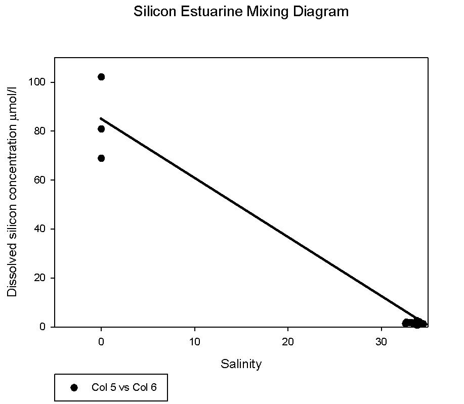
figure 42: silicon mixing diagram through estuary
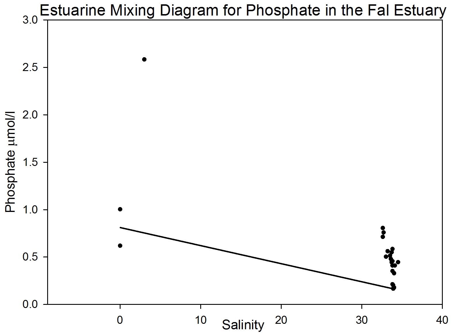
figure 43: phosphate mixing diagram through estuary.
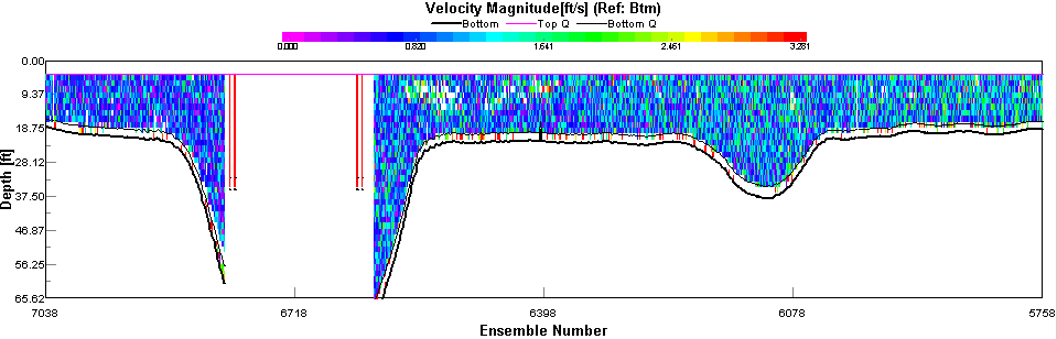
figure 44: velocity magnitude plot of first transect.
figure 45: backscatter profile of third transect.
figure 46: richardson numbers for station 2
figure 47: richardson numbers for station 3
figure 48 richardson numbers for station 4
figure 49: richardson numbers for station 5 |
||||||||||||||||||||||||||||||||||||||||||||||||||||||||||||||||||||||||||||||||||||||||||||||||||||
|
Silicon analysis At station 1 in the St. Just pool (50 10.597N, 005 01.543W) dissolved silicon which was sampled at five depths (surface, 5m, 10m, 16m and24m) can be seen increasing in concentration between 0 and 16m, from 0.80µmol/l to 1.83µmol/l, before again dropping to 0.8µmol/l at 24m depth. Salinities are fairly uniform with depth at this station only varying by 0.2. At station 2 three depths were sampled, surface, 4m and 11m. Silicate peaks at 2.0µmol/l at 4m suggesting that removal may take place by diatoms in the surface waters followed by recycling at around 4 m depth. Concentration then drops to 1.2µmol/l at 11m. Salinities vary from 33.8 at the surface to 34.5 at 11m, suggesting there is a slightly fresher, more nutrient rich layer overlying the more saline sea water below, which explains why nutrient levels at depth are lower. Station 3 was sampled at four depths, 0, 3, 6 and 12m. As with station 2 the highest concentration of silicate is observed in intermediate depths, increasing from 1.4 – 2.5 µmol/l between 3 and 6m depth. This corresponds to the CTD flouresence data which suggests a peak in chlorophyll between 3 and 4m depth (figure 37) before dropping to a minima between 6 and 7m depth. The lowest silicate value is again observed from the deepest sample. Station 4, in shallow waters was only sampled at 0, 1.5 and 3.4m. Concentration only varies by 0.13, suggesting total mixing throughout the water column which can be supported by the CTD data (figure 39). At station 5 only two samples were taken; surface and 2m depth. Silicate levels at the surface are lower (1.37µmol/l) than at 2m, (1.92µmol/l) implying that there is more removal by diatoms here. The estuarine mixing diagram for silicon, with a line plotted through an average of the contributing riverine end members, shows that silica behaves non-conservatively in the area of the estuary studied (see figure 42). The mixing diagram suggests that silica is being removed from the estuary as the points fall below the theoretical dilution line. This could be accounted for by biological activity in the estuary, such as uptake by diatoms which use silica to build their frustules. |
|||||||||||||||||||||||||||||||||||||||||||||||||||||||||||||||||||||||||||||||||||||||||||||||||||||
|
Phosphate analysis Estuarine systems are dynamic and have many factors influencing the chemistry of the water. For this reason, low concentration nutrient values such as those recorded for phosphate are very variable and show a large degree of scatter. The estuarine mixing diagram (figure 43) shows a theoretical dilution line linking an average of two Truro River tributary end members the river Allen and river Kenwyn to the saline end member. The Truro River end member was very high, possibly as a result of an anthropogenic input. However further down the estuary there is a sewage works with the possibility of sewage outfall from the sewage works on the west bank of the river Truro located at 50° 14′ 58.14″ N 5° 2′ 29.55″ W (www.Geolocation.ws). Other possible reasons for the differences in phosphate concentrations between the rivers include the catchment area – an urban area would be likely to have a low phosphate input into the river system than an area with lots of arable farmland where the use of fertilisers run off into the rivers causing a high input of phosphate. The saline end member used is not the value with the highest salinity but the one with the lowest phosphate concentration. The reason for this is that the phosphate concentration recorded for the most saline sample was unusually high and so was likely to have been influenced by some anthropogenic input as described above (pers. comm. P. Statham). Plotting the theoretical dilution line in this way indicates that there were inputs of phosphate to the estuary causing non-conservative addition to occur. Without further information and a more detailed survey it is difficult to state what inputs are active, but in an estuarine system anthropogenic inputs and biogeochemical processes are important. Resuspension of reducing sediments is one likely cause for elevated phosphate concentrations recorded at lower depths. As pore waters are resuspended they add phosphate to the water column and further mixing results in higher phosphate concentrations in the water column (Mortimer et al. 1999). Possible anthropogenic causes for this could be the movement of large vessels through the estuary which disturb and resuspend the sediment. Other natural causes could be due to wind and wave action causing resuspension through mixing. Phytoplankton distributions also have an impact on phosphate concentrations, although they take up phosphate and reduce the concentration they are an important factor in phosphate concentrations. For example looking at (figure 37) it shows a lower phosphate concentration where there is a high chlorophyll level, indicating that plankton are utilising the phosphate and reducing the concentration. Another process by which phosphate levels are reduced is adsorption onto particles such as iron oxides which removes the phosphate from the water column. With regards to phosphate distribution at station 1 (figure 35) the phosphate concentrations are lower at 10metres than the surface but are higher at 16m and then lower at 25m. This would indicate that phosphate has been utilised by plankton in the upper layer and then resuspension may have occurred at the seabed which means that phosphate may have been absorbed onto particles leaving a phosphate rich layer at 16m. Station 2 (figure 36) shows phosphate concentrations are relatively similar showing a slightly higher value at the seabed than the surface which can probably be explained by biological activity. At station 3 (figure 37) there is a lower phosphate concentration at the seabed than the surface but a higher phosphate level below the chlorophyll maximum. At station 4 (figure 39) phosphate concentrations are relatively similar with a higher concentration at 1.5metres this could be an anthropogenic input but without further detail it is difficult to explain this change. At station 5 (figure 40) phosphate levels are again relatively similar but the water was not deep enough to observe a substantial change throughout the column. In general moving up the estuary from station 1 to station 5 there is an increase in phosphate concentration. This is expected as the further inland the estuary is the more inputs of phosphate there are into the river. |
|||||||||||||||||||||||||||||||||||||||||||||||||||||||||||||||||||||||||||||||||||||||||||||||||||||
|
Zooplankton For the analysis of the zooplankton, we followed the same method of analysis as in the offshore survey. However, for the calculation of the volume of water that has been sampled a flow meter was used at all stations except at station 5. At station 5 the flowmeter got stuck and so the volume of water passing through the net was calculated using the ADCP transect velocity in combination with the vessel speed to calculate the flow past that point. At station 1 a plankton trawl was taken across the estuary, whereas at stations 2 and 5 a trawl was taken across the area of transect for a fixed amount of time. The tidal current at station 5 was strongest and so the most water was sampled here. All of the values indicated for zooplankton numbers were taken per m-3 and these were graphed to show the variation in zooplankton type between each of the stations. Station 1, which was located closest to the seawater end member, has the greatest amount of zooplankton per unit area whereas, station 5, which was located furthest away from the seawater, and so also had the lowest salinity. This could be explained by the lower salinities and so a lower tolerance at the top of the estuary. A greater tolerance to a range of salinities is exhibited by fewer species and individuals, according to Remane’s species salinity relationship, thus explaining the distribution of zooplankton up the estuary. At all stations the dominant zooplankton was copepod nauplii with only few adult individuals. This can be explained by the fact that copepod nauplii are associated with summer plumes of nutrients common in estuaries (Dagg and Whitledge,1991). At station 1, hydromedusae were relatively abundant as well with 43 individuals per m-3 (see figure 38). The abundance of hydromedusae here can be attributed to the fact that hydromedusae are common in estuaries in summer environments (Marques et al, 2007). A general shift in the type of zooplankton can be seen, from almost equal amount of hydromedusae and copepod nauplii at the bottom of the estuary, to copepod nauplii being by far the most dominant further up the estuary. Other types of zooplankton were in the minority and only existed in limited numbers or not at all in the estuary. This shows that due to the lower salinities, experienced in the estuary, only certain types of organisms can tolerate these conditions and exist here. |
|||||||||||||||||||||||||||||||||||||||||||||||||||||||||||||||||||||||||||||||||||||||||||||||||||||
|
ADCP Transect 1 (Start: 50 10.324N 005 02.671W Finish: 50 10.629N 005 01.259W) started at 07:42 and ended at 07:55GMT. The velocity magnitude ranged from 0.09m/s to 0.375m/s across the transect. The lowest velocities occurred at the mouth of the Restronguet Creek at the transect end (see figure 44). The velocity direction only changed at the estuary edges where shear occurred and the average direction changed from 17° to 183°. The backscatter taken from the ADCP indicated far greater biological activity or suspended sediment in the middle of the estuary (average of 75dB) when compared to the sides (average 68dB). Transect 2 (Start: 50 12.299N 005 02.239W Finish: 50 12.255N 005 02.138W) started at 08:50 and ended at 08:53GMT. The velocity magnitude changed with the depth of the estuary from 0.102m/s to 0.186m/s at 15m. The backscatter showed a small amount of reflection (71dB average) at 10m indicating plankton activity which coincided with the 1% light depth. Transect 3 (Start: 50 13.432N 005 01.580W Finish: 50 13.367N 005 01.430W) started at 9:42 and finished at 9:45GMT. The velocity magnitude remained constant throughout with an average of 0.142m/s. The velocity direction changed throughout the water column moving in all directions due to the shallow depth of the water causing shear. The backscatter values indicated suspended sediment and plankton to be equally distributed in the water column (see figure 45). Transect 4 (Start: 50 13.847N 005 00.962W Finish: 50 13.806N 005 01.075W) started at 10:06 and finished at 10:08GMT. The velocity magnitude remained constant at 0.173m/s. The flow direction was South West. The backscatter indicated the highest values 1m from the seabed with an average of 71dB signifying an abundance of suspended sediment. Transect 5 (Start: 50 14.347N 005 00.837W Finish: 50 14.361N 005 00.964W) started at 10:22 and finished at 10:24. The velocity magnitude was constant throughout the estuary with an average of 0.234m/s. The velocity direction was South West and the backscatter recorded values of 75dB throughout the water column signifying suspended sediment and plankton in high numbers. |
|||||||||||||||||||||||||||||||||||||||||||||||||||||||||||||||||||||||||||||||||||||||||||||||||||||
|
Richardson's Number The Ri numbers were calculated using the same formula as the offshore calculations (offshore). Station 1 was too deep for the ADCP to take any readings so no Ri number was calculated. Station 2 showed mostly unstable flow with 2 points of stability at 2m and 7m (see figure 46). This indicates a well-mixed area which is supported by the CTD data indicating no sharp changes in temperature or salinity (see figure 36). Station 3 was split in terms of stability with the water maintaining stable flow down to 4m when it became unstable, Ri 0.069. From 5-8m the Ri was greater than 1 and beyond that the flow became gravitationally unstable (see figure 47). The CTD data shows a small amount of stratification by salinity (an increase of 7), at the surface, where the flow was stable. Station 4 shows mixing throughout the water column with all Ri values below 1 (see figure 48). The CTD reflects this with no significant changes occurring in any of the data sets. Station 5 is entirely mixed and has gravitationally unstable flow (see figure 49) over the entire water column which is indicated by the CTD data which remains constant from surface to seafloor.
|
|||||||||||||||||||||||||||||||||||||||||||||||||||||||||||||||||||||||||||||||||||||||||||||||||||||
| Fal Estuary Residence Times Smean= averaged estuarine salinity from the 5 stations sampled, using a YSI probe Ssea= Salinity of marine end member from deepest point measured at black rock Vtotal= total volume of the Fal estuary water 1.36×10⁷ m3 (rough estimation from Admiralty charts 5602.5 and 5602.3). R= Annual average of daily river flow rates m3s-1. River Fal: 2.041 m3s-1 (1978-2009 average), River Kenwyn 0.38 m3s-1 (1968-2009 average) (CEH 2011). Tres= residence time in seconds Tres = ((1-33.6/35.2)*13600000)/2.421 = 255341.5s =70.93 hours The residence time calculated is an overestimate as flow rates of other tributaries and inputs, in particular the Tressilian and Allen rivers are not taken into account. The high mean salinity (33.6) shows that there is low freshwater content which is quickly flushed by tidal movements.
|
|||||||||||||||||||||||||||||||||||||||||||||||||||||||||||||||||||||||||||||||||||||||||||||||||||||
| Conclusion | |||||||||||||||||||||||||||||||||||||||||||||||||||||||||||||||||||||||||||||||||||||||||||||||||||||
|
From the estuarine analysis several conclusions can be drawn. Zooplankton showed a clear trend towards more tolerant species in the estuary, with a decrease in salinity showing a decrease in abundance as well. Chlorophyll has a less profound trend with a chlorophyll maximum at around 10m for all stations except station 5, which had the maximum at the surface; the Secchi depths, at stations 3, 4 and 5, tell us that there is sufficient light for all growth to the bottom of the estuary. The nutrient data helps in explaining these trends with dissolved oxygen accounting for higher numbers of chlorophyll and the lower numbers of silicate and phosphate accounting for the scavenging out of these nutrients by the phytoplankton. We can also see that the Fal estuary was well mixed. However, when looking at data for estuarine systems it is important to remember that the systems are transient and subject to a great deal of change over short time spans. For this reason care must be taken when considering patterns shown by the data, as they may not be permanent features. |
|||||||||||||||||||||||||||||||||||||||||||||||||||||||||||||||||||||||||||||||||||||||||||||||||||||
| Conclusion |
| On the Falmouth trip 2011 a range of data collection techniques were employed to build up a picture of the biological, chemical and physical processes active in the Fal Estuary and surrounding offshore waters. In the offshore survey, differences were observed between well mixed and stratified waters, fulfilling the aim of examining changes in parameters across a front. A benthic habitat map and information on benthic flora and fauna was collected as part of the geophysics survey. In particular, the St. Mawes maerl beds were sampled using grab samples and sidescan sonar. The limited salinity range of the estuary was one of the most noticeable factors of the estuarine survey. As a result of the many processes with the capacity to influence estuarine chemistry, further study into the nutrient distributions would be necessary to give a definitive reason for the chemical distributions. As further investigation, we would have found it interesting to be able to do more samples along the front to explore further the front characteristics. In addition, samples from further up the river at lower salinities would have been useful to extent the dissolved nutrient data collected, but this was not possible with the time and equipment available at the time. However, in combination the three studies undertaken give an overview of the area which can be compared to the work of other groups and that of previous years to give a more detailed picture.
|
| References |
| Introduction Exeter University, n.d.. The Wheal Jane incident and water quality. [online] available at: http://projects.exeter.ac.uk/geomincentre/estuary/Main/jane.htm [01/07/2011] JNCC, 2000. Fal and Helford: Natura 2000 data form. [online] available at: http://jncc.defra.gov.uk/ProtectedSites/SACselection/n2kforms/UK0013112.pdf[02/07/2011] Macadam, J.D., Edwards, T., Richards, H.V., Pine, R.J., 2003. The last 3 years out of 400 million: a progress report from Cornwall, UK. Geoparks conference Poster. Pirrie, D., Camm, G.S., Sear, L.G., Hughes, S. H., 1997. Mineralogical and geochemical signature of mine waste contamination, Tressilian river, Fal estuary, Cornwall, UK. Environmental Geology 29(1) pp.: 58-65. Lab Methods YSI. Accessed online at http://www.ysi.com, (no date), [08/07/2011] Strickland, j.d., and Parsons, t.r (1968). Determination of dissolved oxygen. Fisheries Research Board of Canada, Bulletin. 16: 71-75. Winkler,L.W. (1888). Die Bestimmung des in Wasser geolsten Sauerstoffen. Berichte Deutschen Chemischen Gesellschaft, 21: 2843-2855. Offshore Harris, R.P., 1988. ‘Interactions between Diel vertical migratory behaviour of zooplankton and the subsurface chlorophyll maximum’. Bulletin of Marine Science, 43, 3,663-674. Hawkins, S.J., Southward, A.J. and Genner, M.J., 2003. ‘Detection of environmental change in a marine ecosystem – evidence from the Western English Channel’. Science of the Total Environment, 310,1-3, 245-256. Hirst, A.G., Bonnet, D., Harris, R.P., 2007. ‘Seasonal dynamic and mortality rates of Calanus helgolandicus over 2 years at a station in the English Channel’. Marine Ecological Progress Series, 340, 189-205. Holligan, P.M. and Harbour, D.S., 1977. ‘The vertical distribution and succession of phytoplankton in the Western English Channel in 1975 and 1976’. Journal of Marine Biological Association U.K., 57, 1075-1093 Knauss, J.A., (1997). Introduction to Physical Oceanography. Waveland Press. Nash J. and Moum J. (2005) River plumes as a source of large-amplitude internal waves in the coastal ocean. Nature Vol. 437 pp. 400-403 Rodriguez, F., Fernandez, E., Head, R.N., Harbour, D.S., Bratbak, G., Heldal M., Harris, R.P., 2000. ‘Temporal variability of viruses, bacteria, phytoplankton and zooplankton in the western English channel off Plymouth’. Journal of Marine Biological Association U.K., 80, 575-586. Simpson, J.H., and J, Hunter (1974) Fronts in the Irish Sea. Nature 250, 404-406 Turner, J. S. (1973) Buoyancy Effects in Fluids. Cambridge Uni Press Widdicombe, C.E., Eloire, D., Harbour, D., Harris, R.P., Somerfield, P.J., 2010, ‘Long-term phytoplankton community dynamics in the Western English Channel’, Journal of Plankton Research, 32, 5, 643-655. Geophysics Bird, E. (1998). The Coasts of Cornwall. Alexander Associates, Fowey, Cornwall, 237 pp. Deeble.M &Stone.V (1985). A port that could threaten life in England’s Fal estuary.Oryx.19:74-78. Hall-Spencer J.M & Moore P.G (2000).Scallop dredging has profound, long term impacts of maerl beds.ICES journal of marine science. 57(5):1407-1415. Hayward,p.,Nelson-Smith,T.and shields, C.(1996) .Sea shore of Britian and Europe , Harper Collins Natural England. Accessed online at http://www.naturalengland.org.uk/ourwork/marine/protectandmanage/mpa/mcz/features/habitats/tide-sweptchannels.aspx [08/07/2011] UK Marine SAC. Accessed online at http://www.ukmarinesac.org.uk/communities/maerl/m1_1.htm [08/07/2011] Ocean Explorer. Accessed online at http://oceanexplorer.noaa.gov/explorations/08bonaire/background/auvs/auvs.html [08/07/2011] Leveridge, B.E., Holder, M.T. and Goode, A.J.J. (1990) Geology of the Country around Falmouth. British Geological Survey Memoir, Sheet 352. Pirrie.D, Power M, Rollinson G, Camm S, Hughes S, Butcher A, Hughes P (2003). The spatial distribution and source of arsenic, copper, tin and zinc within the surface sediments of the Fal estuary, Cornwall UK.Sedimentology. 50:579-595. Tyler-Walters, H. & Hiscock, K. (2006) Impact of human activities on benthic biotopes and species. Report to Department of environment, food and rural affairs: from the Marine Life Information Network (MarLIN). Plymouth: Marine Biological Association of the U.K. Estuarine Dagg, M.J. and Whitledge, T.E., 1991, Concentration of copepod nauplii associated with nutrient rich plume of the Mississippi river. Continental Shelf Research, 11(11) pp.: 1409-1423. Geolocation. Accessed online at http://www.geolocation.ws/v/W/4d792b4187865614d5024bf1/sewage-works-on-west-bank-of-truro-river/en [ 08/07/2011] Marques, S.C., Pardal, M.A., Pereira, M.J., Goncalves, F., Marques, J.C., Azeitero, U.M., 2007. Zooplankton distribution and dynamics in a temperate, shallow estuary. Hydrobiologia, 587 pp.: 213-223. Mortimer, R.J.G., Krom, M.D., Watson, P.G., Frickers, P.E., Davey, J.T., Clifton, R.J., 1999, ‘Sediment-Water Exchange of Nutrients in the Intertidal Zone of the Humber Estuary, UK’, Marine Pollution Bulletin, 37, 3-7, 261-279. The centre for ecology and hydrology. Accessed online at www.ceh.ac.uk [8/7/2011] |
| Disclaimer |
|
This website and its contents do not represent the views of the University of Southampton, the National Oceanography Centre Southampton or its staff. |
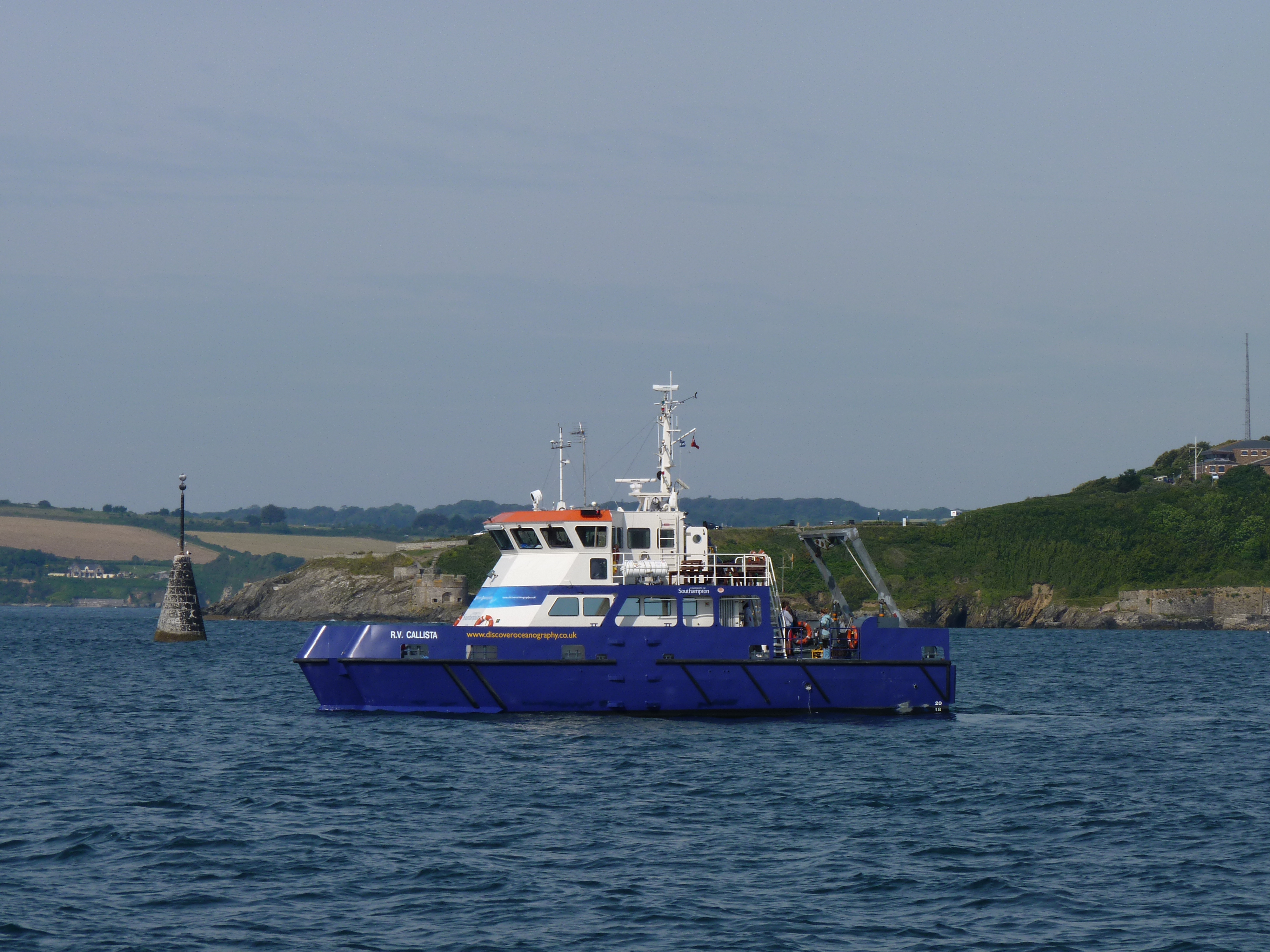
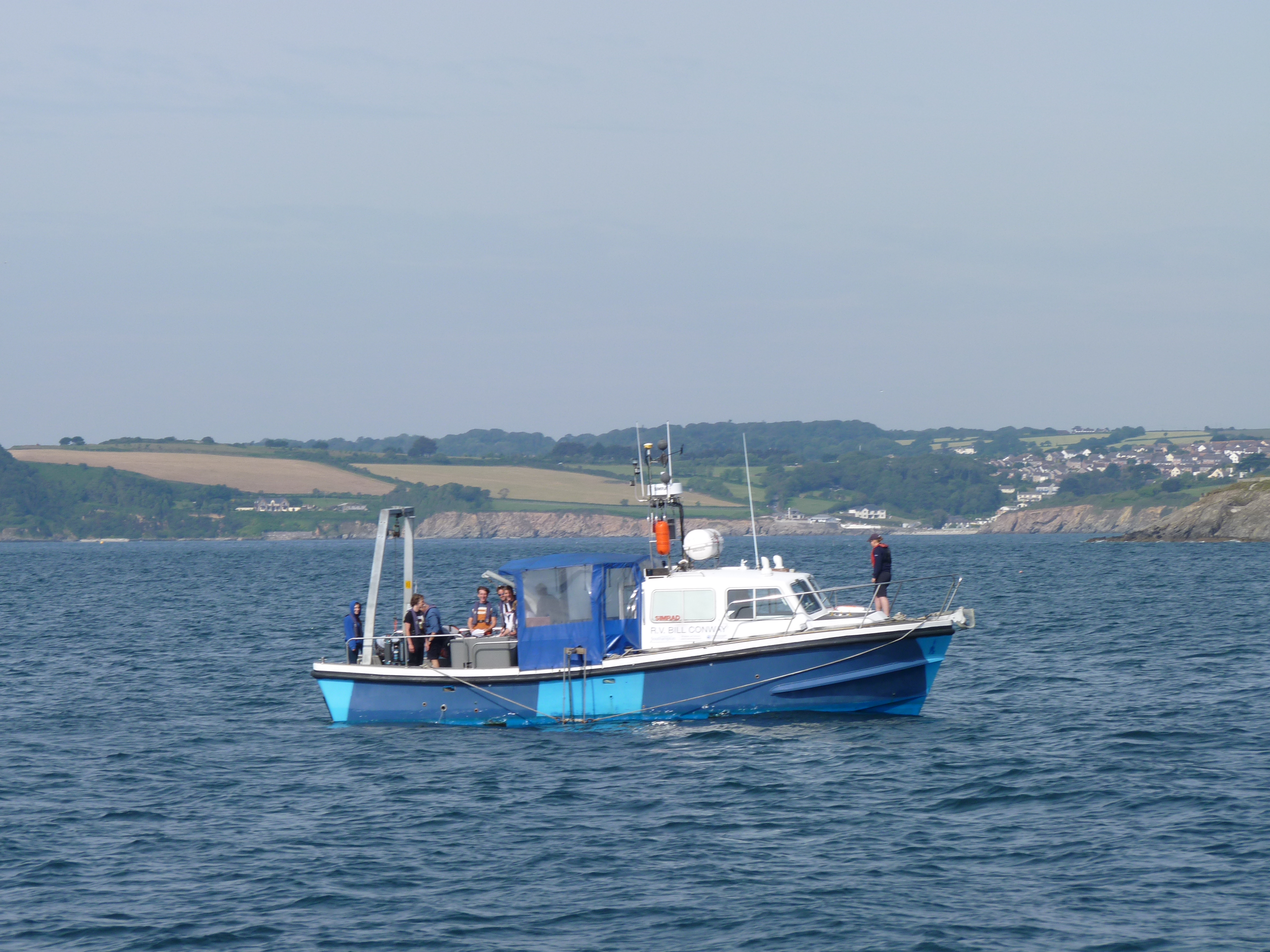
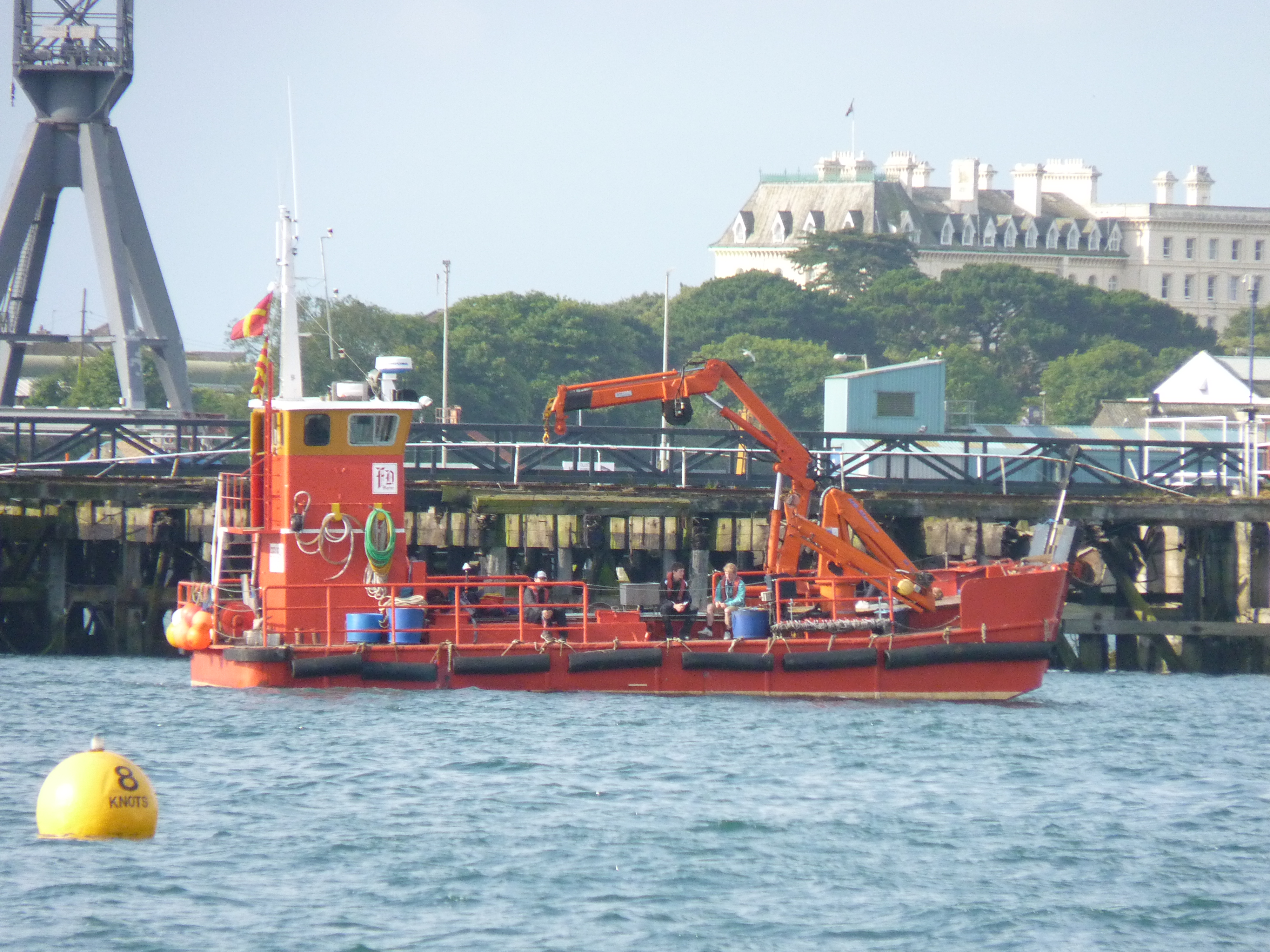
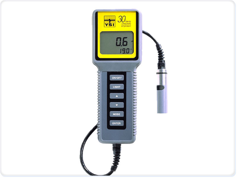
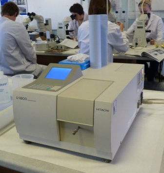
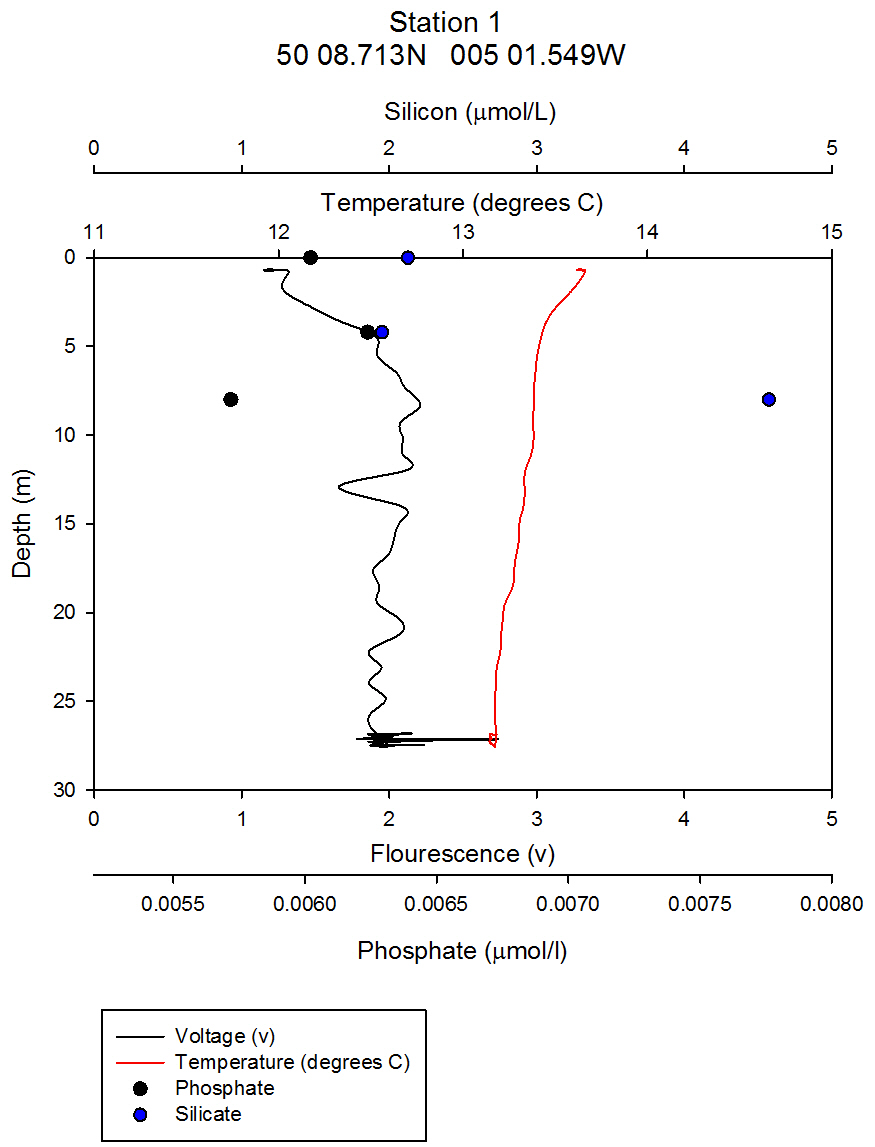
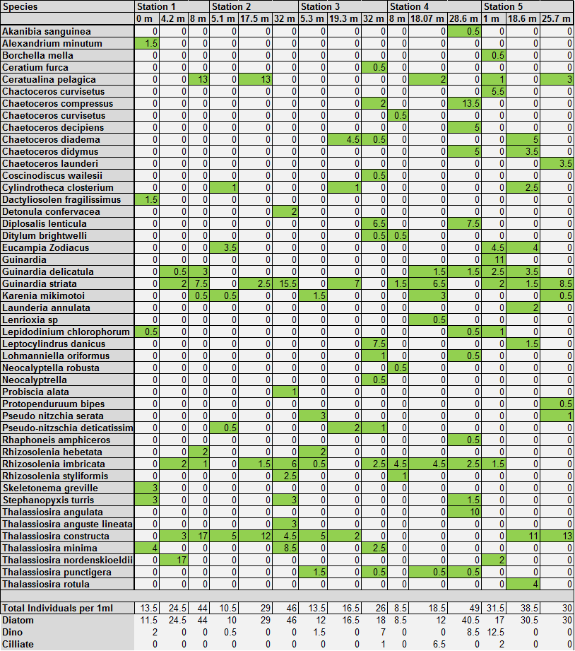
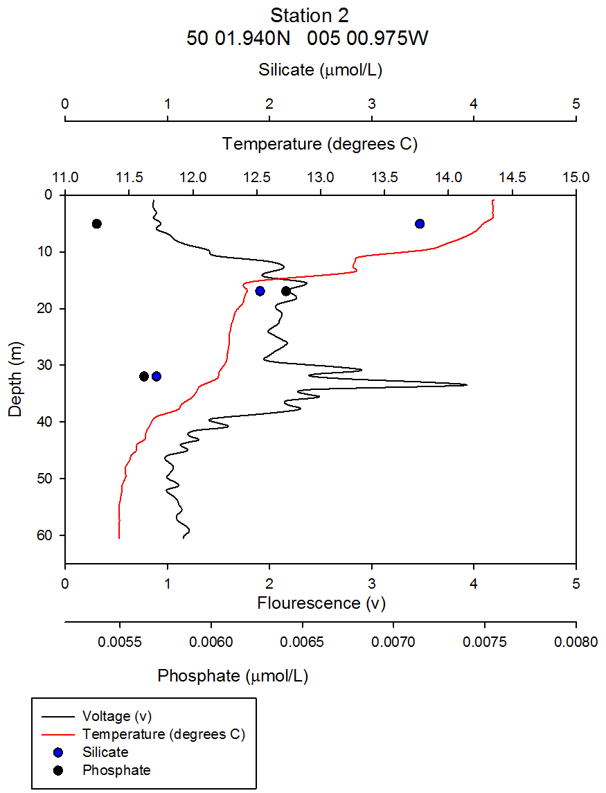
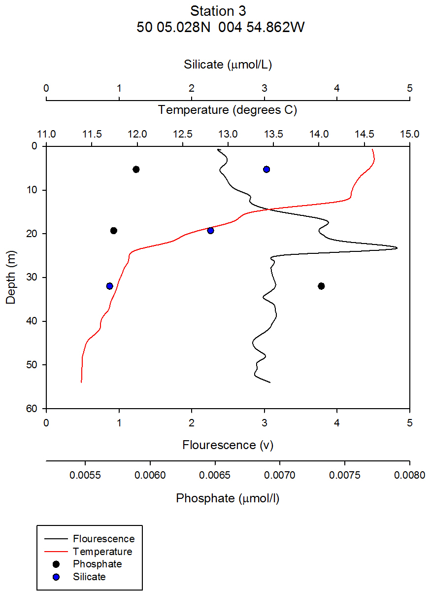
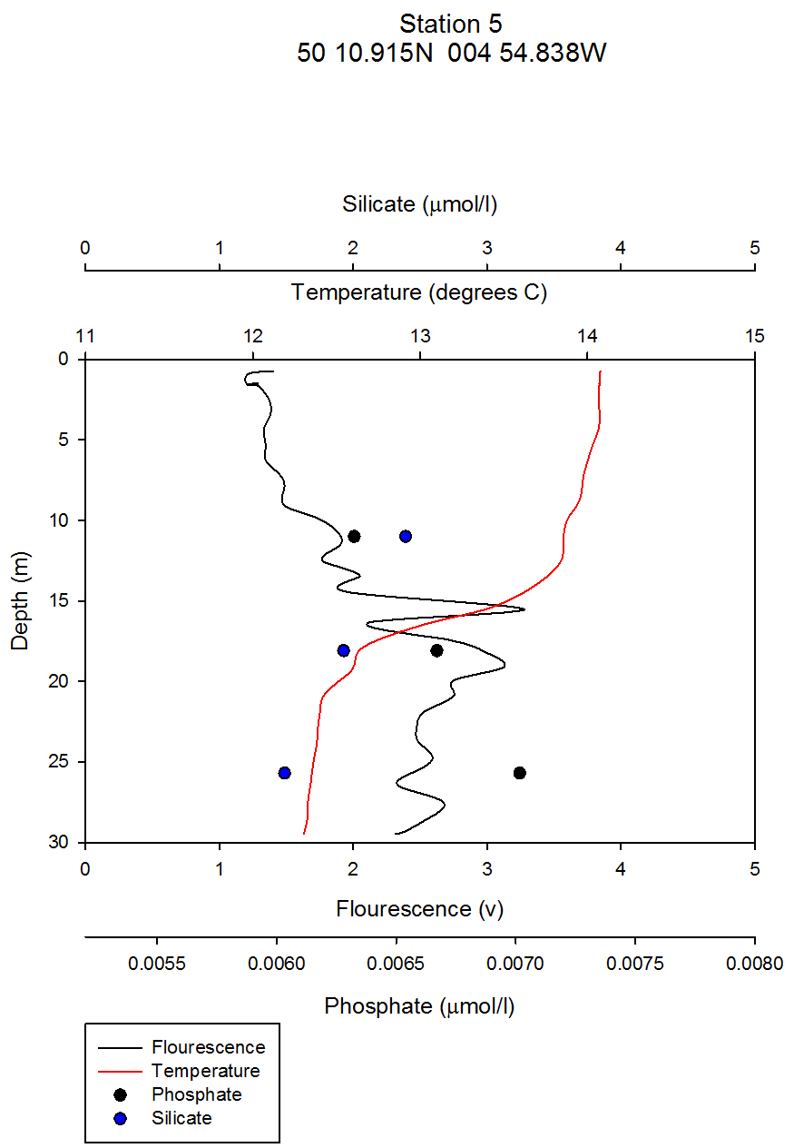
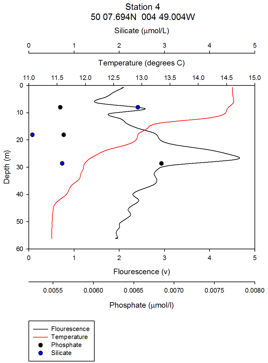
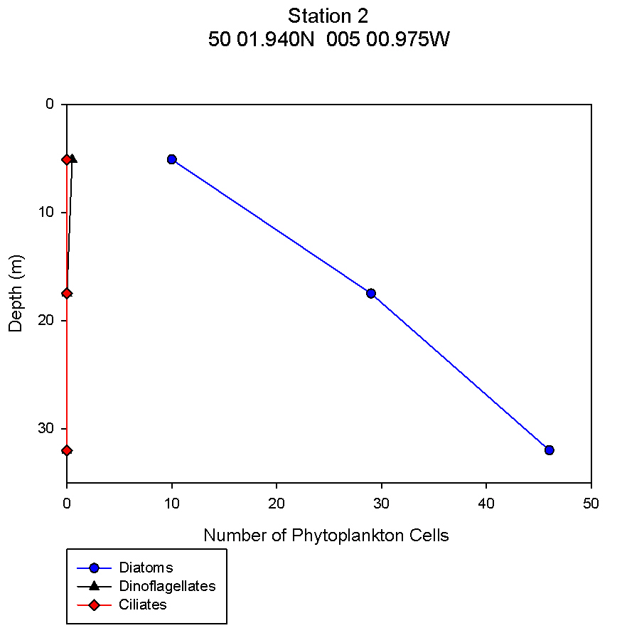
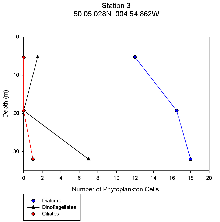
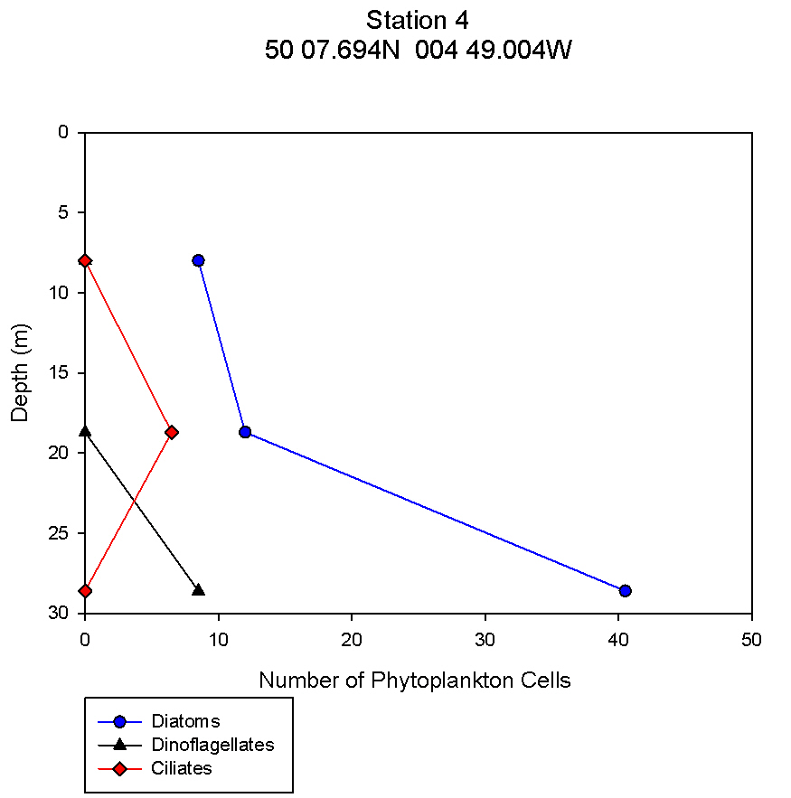
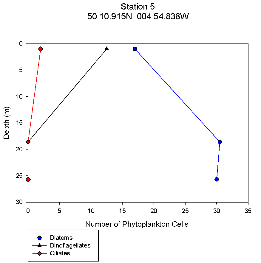
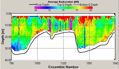
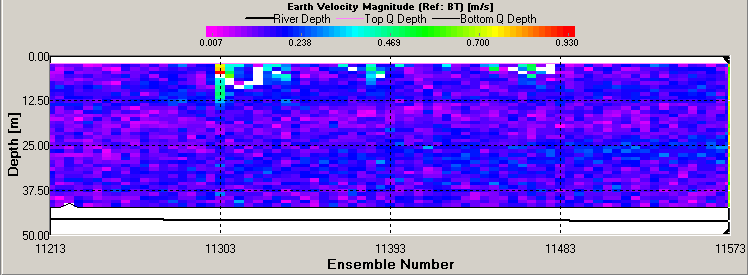
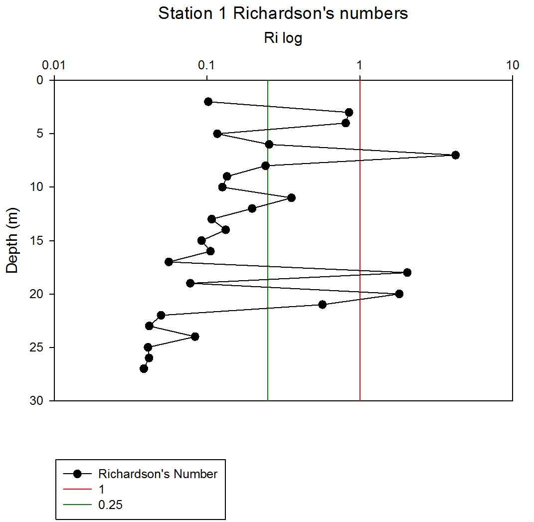
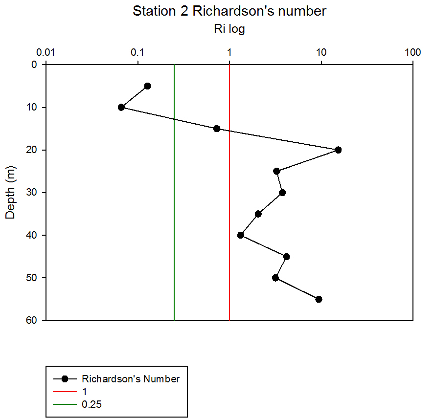
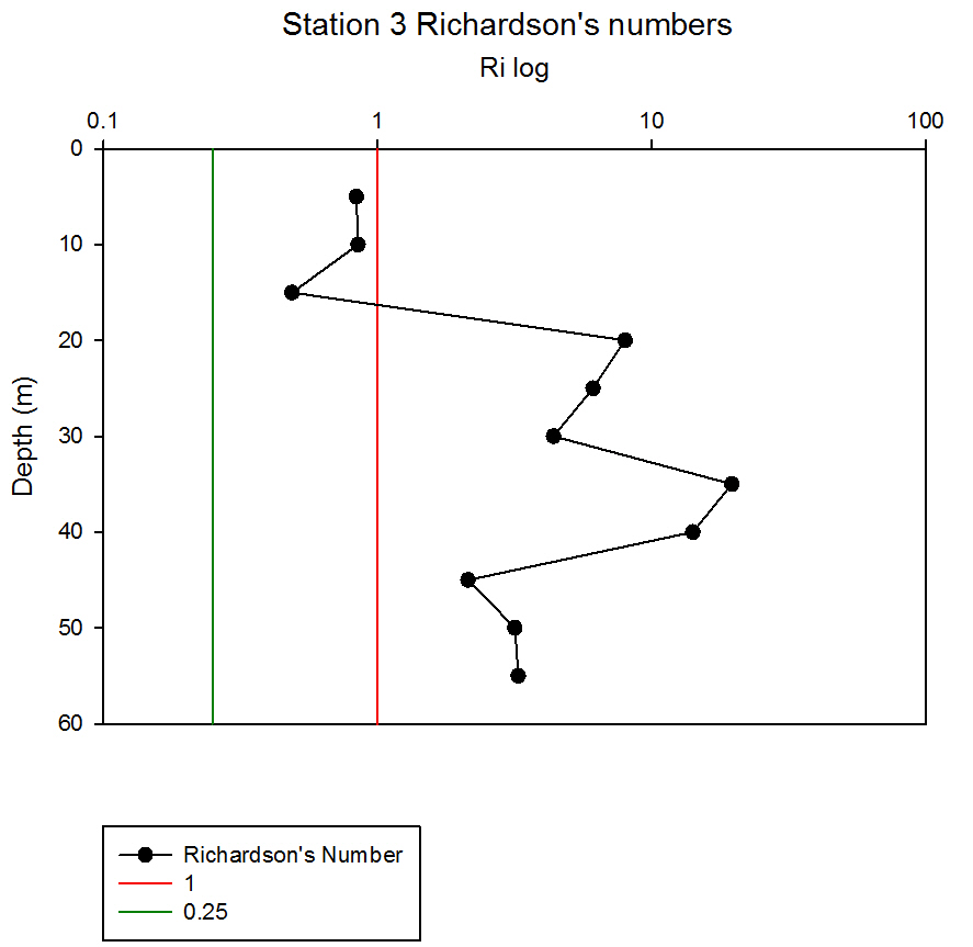
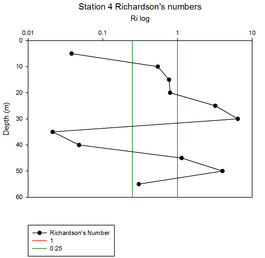
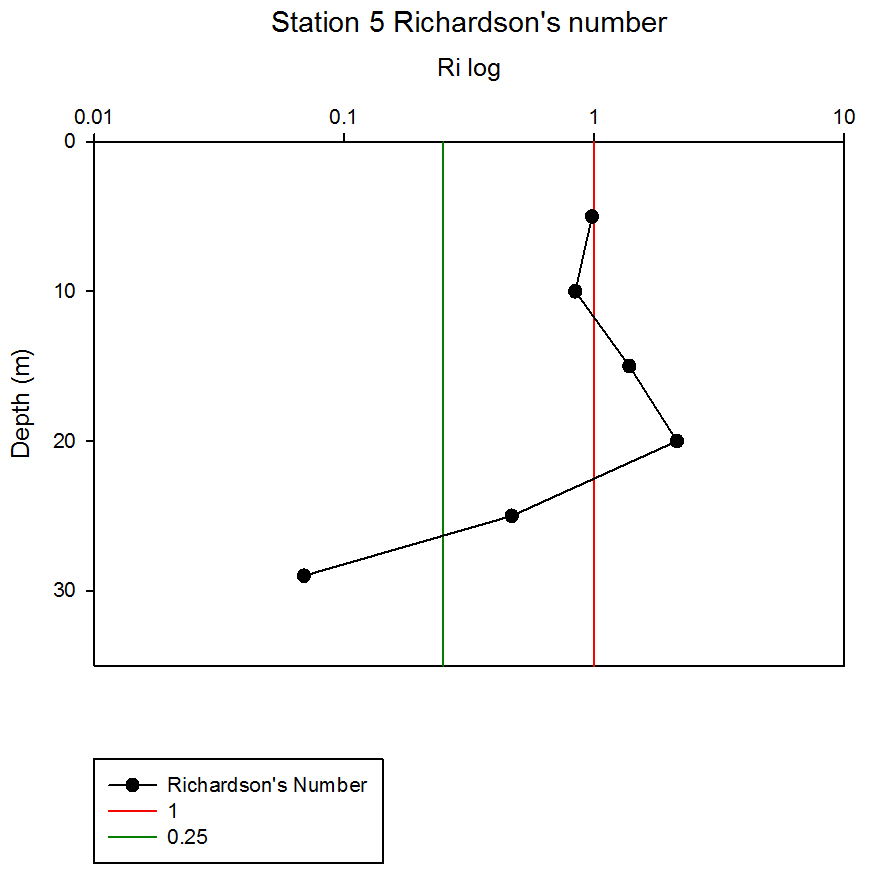
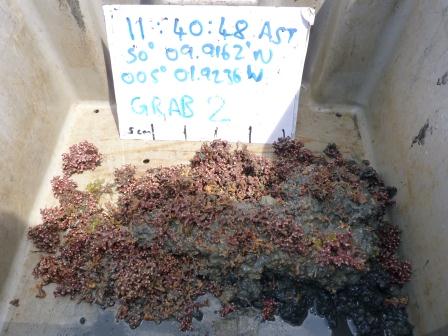
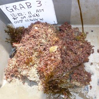
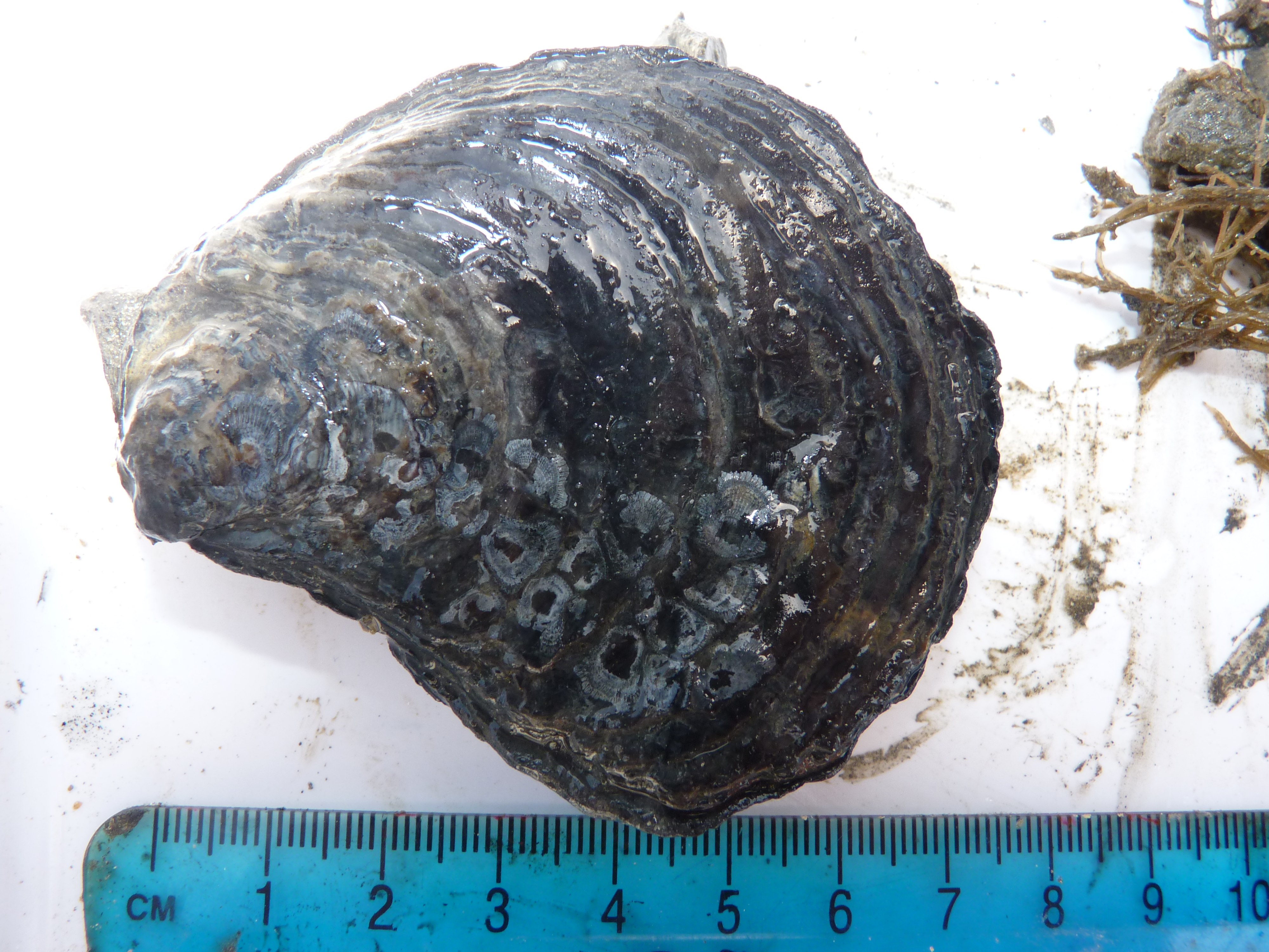

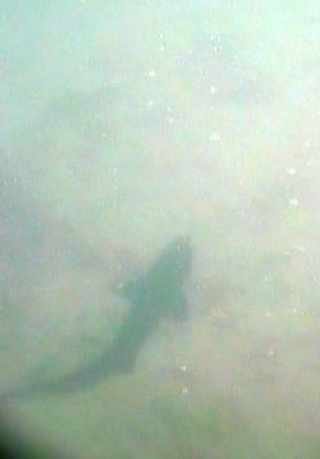
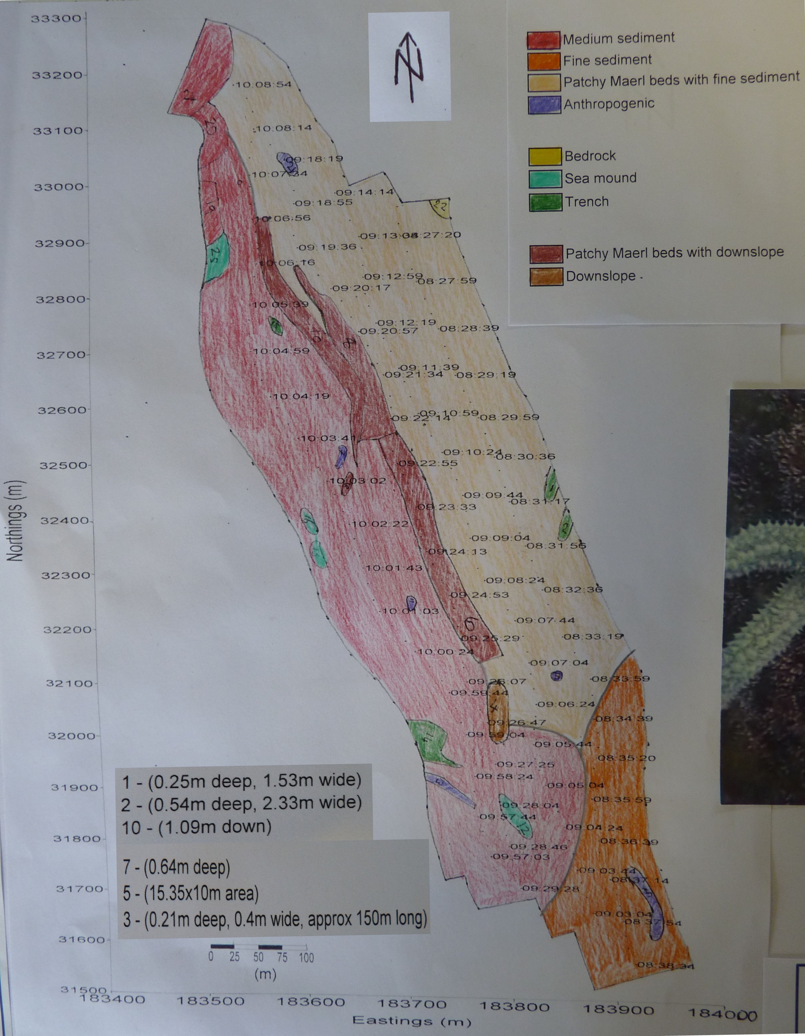
.JPG)
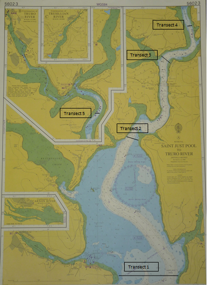
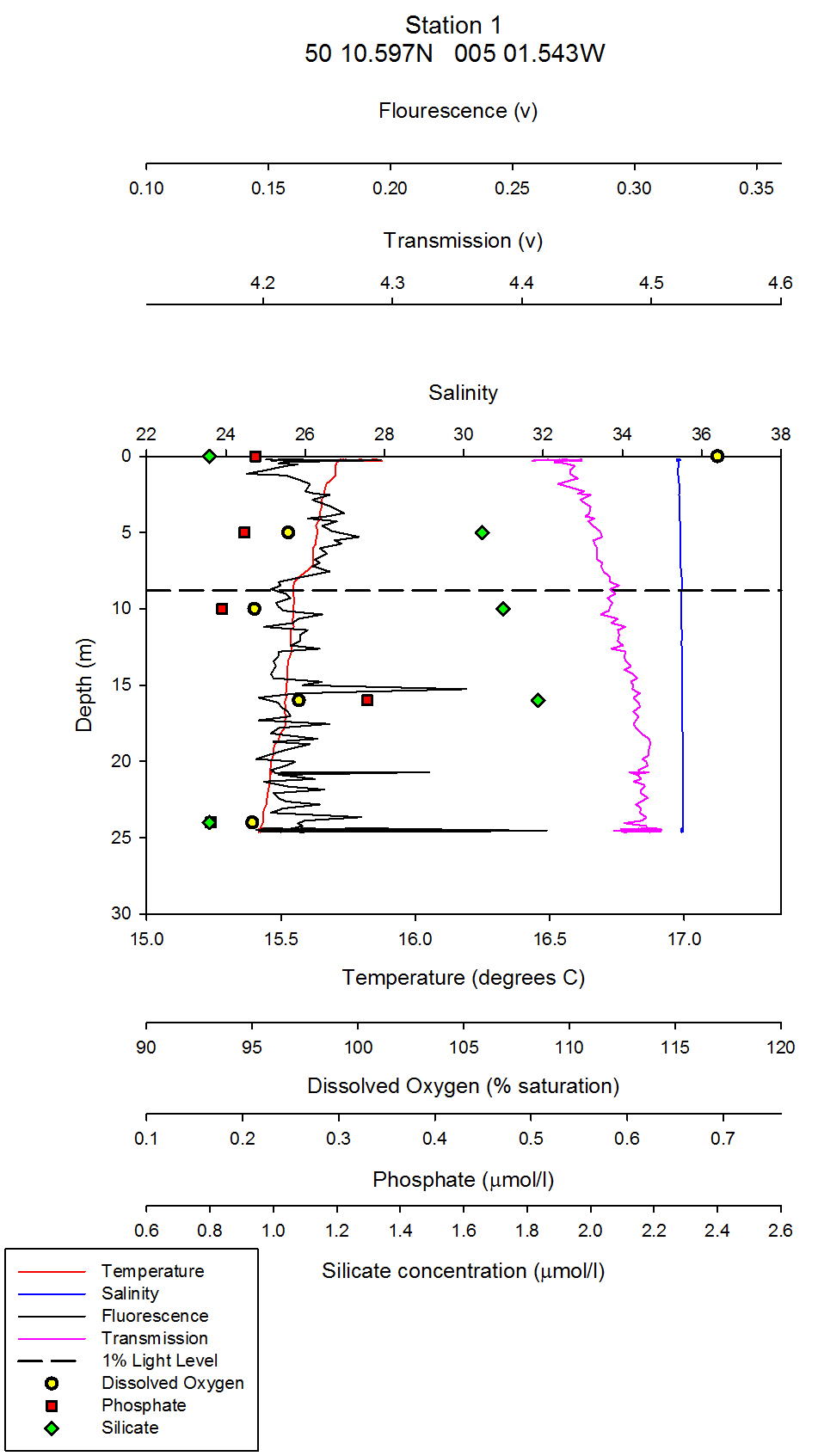
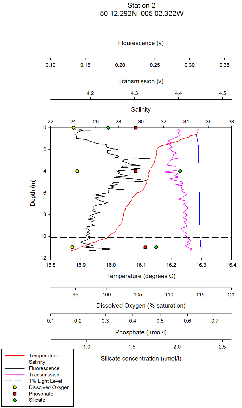
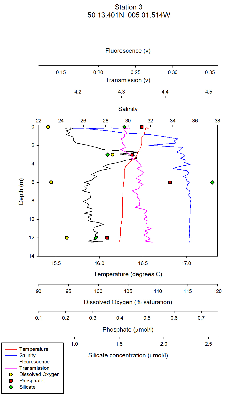
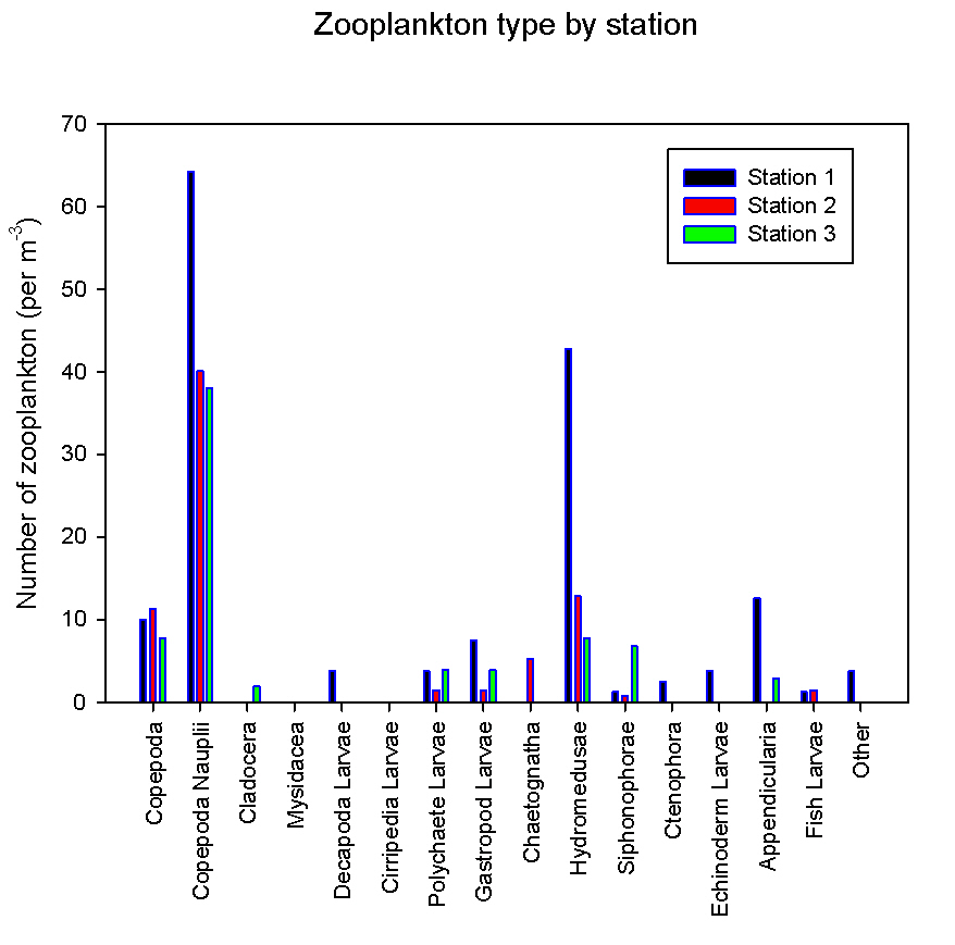
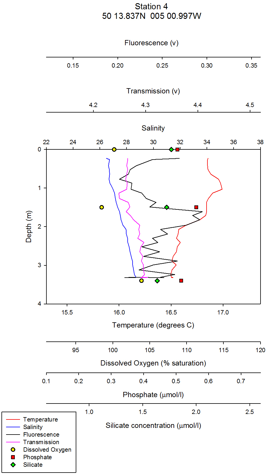
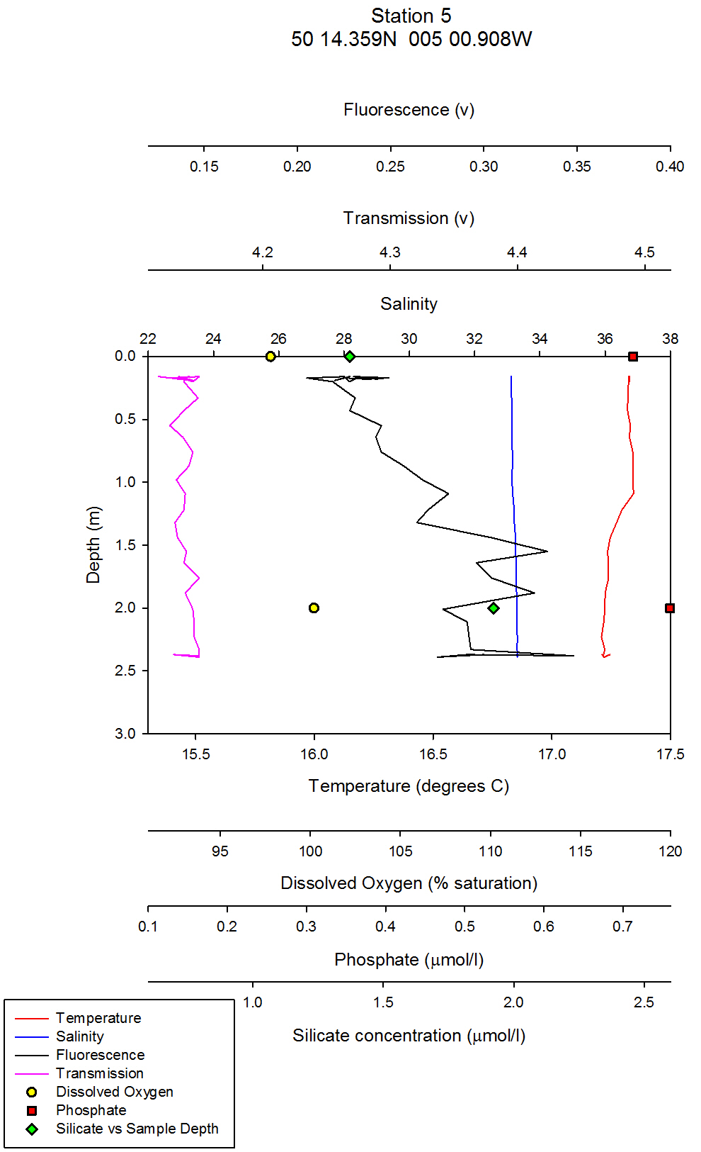

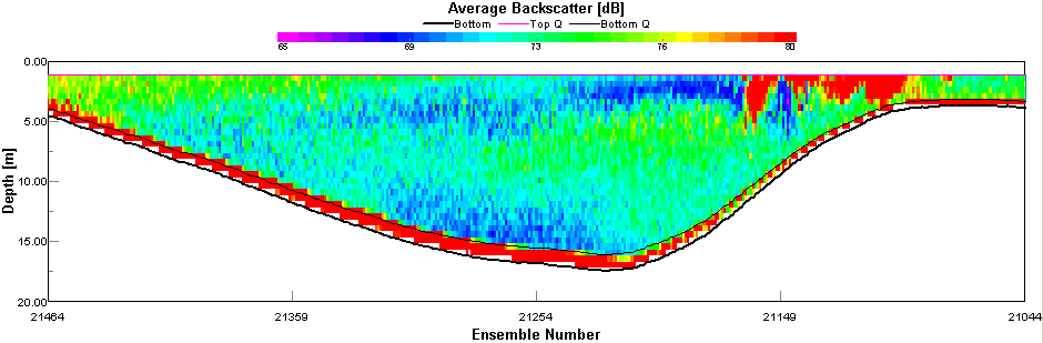
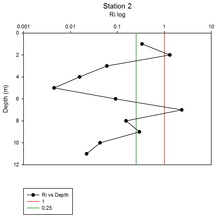
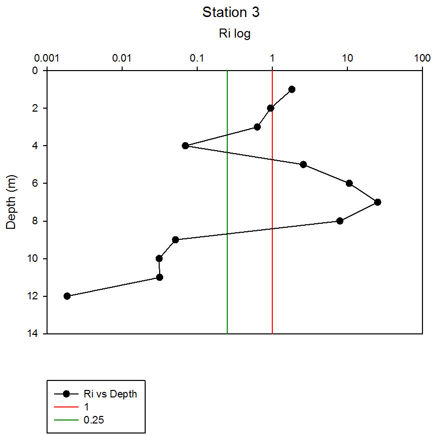
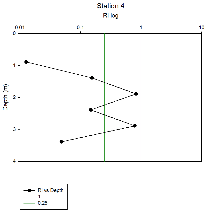
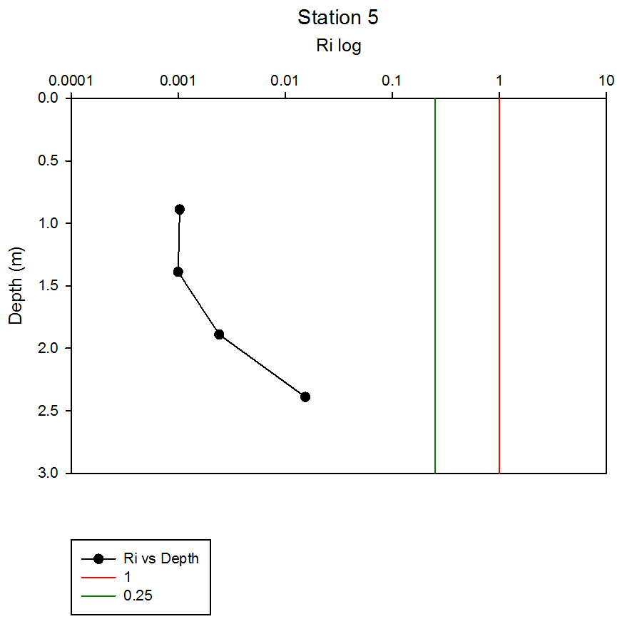
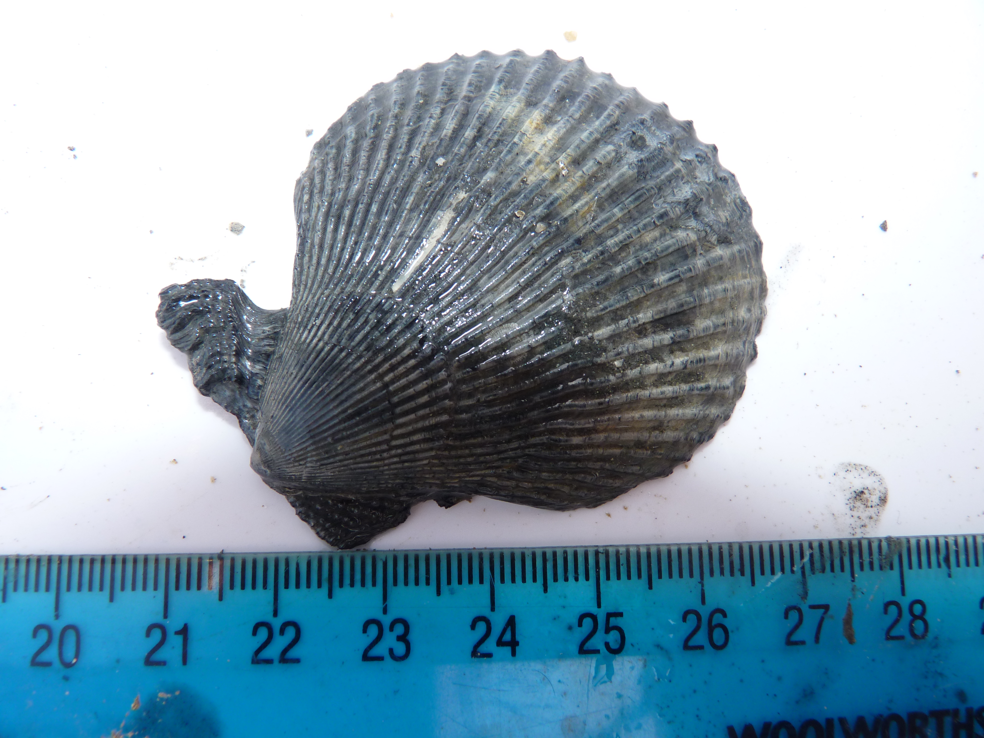
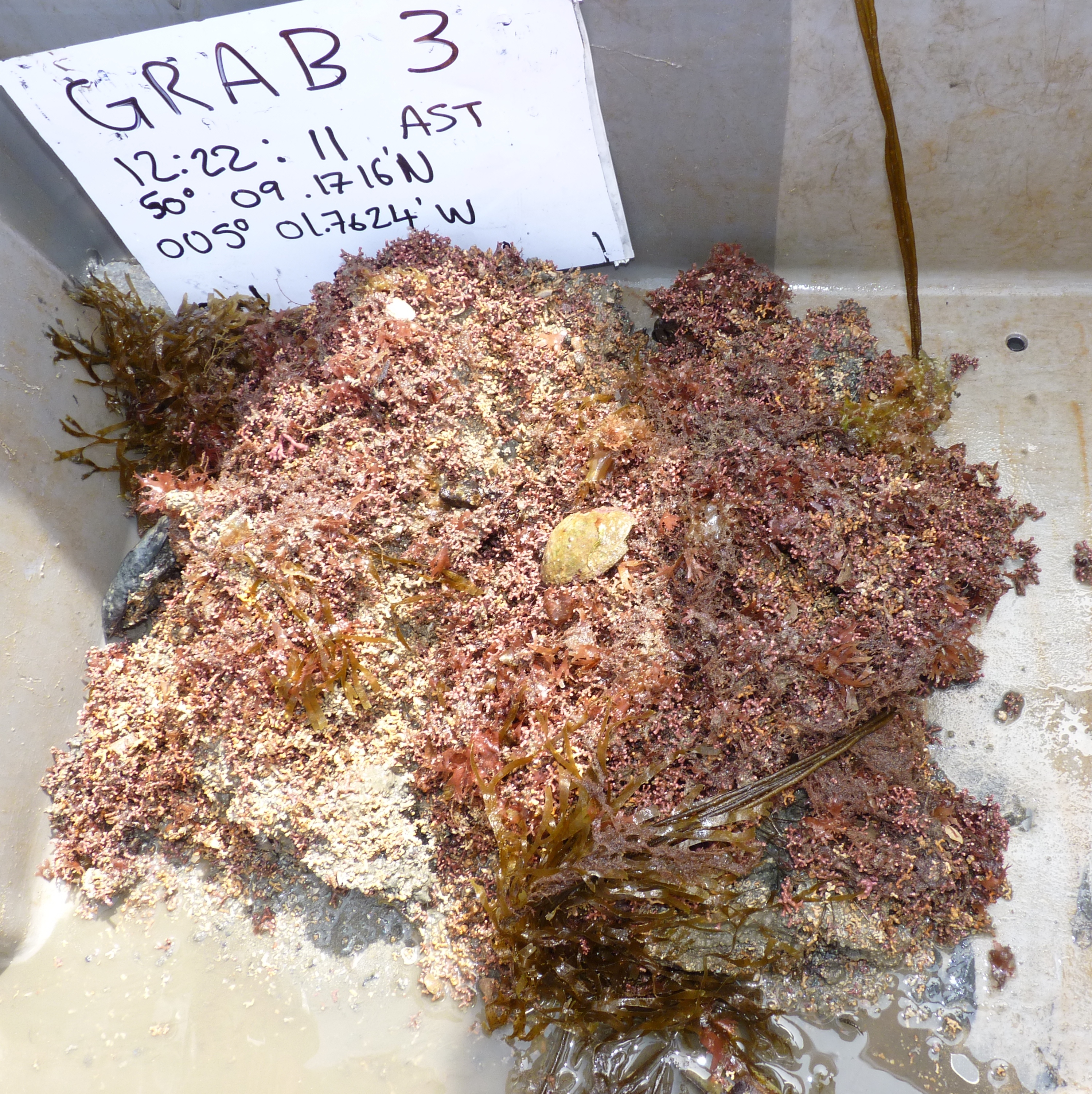