|
From Estuary To Open Ocean: Oceanographic Findings From Falmouth |
 |
|
|
Welcome to Group 6 |
| Gareth Bennett
Madeleine Brasier
Thomas Clarke
Freya Garry
Alex Kesser
|
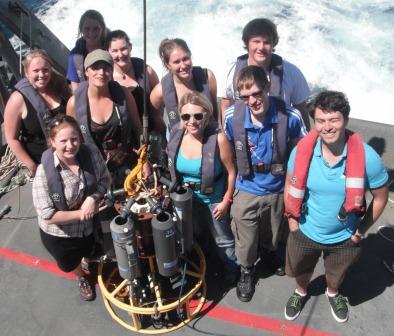
Figure 1.1 |
Lucy Martin
Louisa Payne
Michael Pownall Julia Robinson Suzie Tooke
|
|
|
Intro To Falmouth: Aims & Schedule |
|
This webpage
provides an overview of the scientific procedures and findings
undertaken by Group 6 (Figure 1.1) during a field course in the Falmouth Estuary.
The field course aim was to gain an overview of the physical
chemical and biological systems in the Falmouth area (Figure 2.1). Three boat practicals
were undertaken throughout the fortnight, one in the
Falmouth Estuary, one offshore and one side scan habitat
mapping exercise (Table 2.1). The physical, chemical and biological data
collected during the surveys are processed and integrated to give an
understanding of the estuarine and offshore systems. Particular aims of each
exercise are outlined in the relevant sections below.
The Fal
Estuary is an area of high conservation value with important
biological habitats, for instance maerl beds. The estuary was formed as the
river valley/ria became flooded. As a consequence there is a deep
channel in the centre of the estuary. The geology of the area which
principally comprises of Carnmellis granite and other metamorphic rocks
to the west of the Fal influence the characteristics of the estuary.
Due to the high levels of mining in the past, Restronguet Creek
-which leads onto the Fal Estuary- has become the most metal
polluted estuary in the UK and this has caused contamination of the
sediments in other parts of the Fal. The Wheal Jane mine discharge
in 1992 is a notable source of contamination, but residual drainage
and leakage from spoil heaps lead to contamination of Restronguet
and therefore the Fal (Langston et al. 2003).
The Fal Estuary, a
busy harbour economically and recreationally, is subject to various
pressures from pollution, for instance from organotin contamination
originating mainly from Falmouth Dockyard. Industry and dredging, as
well as sewage and contamination from tri-butyl tin, are additional
anthropogenic factors that affect the physical, chemical and
biological characteristics of the estuary. The Fal Estuary is
generally high in nutrients, leading to hyper nutrification and risk
of eutrophication in parts of the estuary (Langston et al. 2003).
Falmouth is
additionally an ideal base from which to conduct offshore surveys in
the Western English Channel. The vertical mixing processes in the
Channel can be studied whilst aiming to discover how this affects the
plankton communities in the region, with particular reference to the
change in stratification around tidal fronts. |
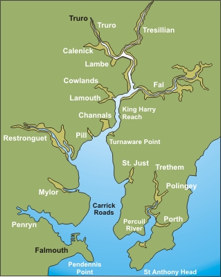
Figure 2.1 |
|
Date |
Description |
| 28/6/2011 |
Web Prep am |
| 29/6/2011 |
Estuarine Boat |
| 30/6/2011 |
Chem Lab am
Bio Lab pm |
| 1/7/2011 |
Data Lab |
| 2/7/2011 |
Offshore Boat |
| 3/7/2011 |
Catch Up Day |
| 4/7/2011 |
Bio Lab am
Chem Lab pm |
| 5/7/2011 |
Data Lab |
| 6/7/2011 |
Geophys boat |
| 7/7/2011 |
Geo Data |
| 8/7/2011 |
Data Lab |
| 9/7/2011 |
Submit Web page |
Table 2.1 |
|
|
Boats & Equipment
|
|
R.V Callista
|
R.V Conway |
L.C. Grey Bear |

Figure 3.1 |
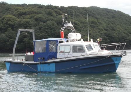
Figure 3.2 |

Figure 3.3 |
|
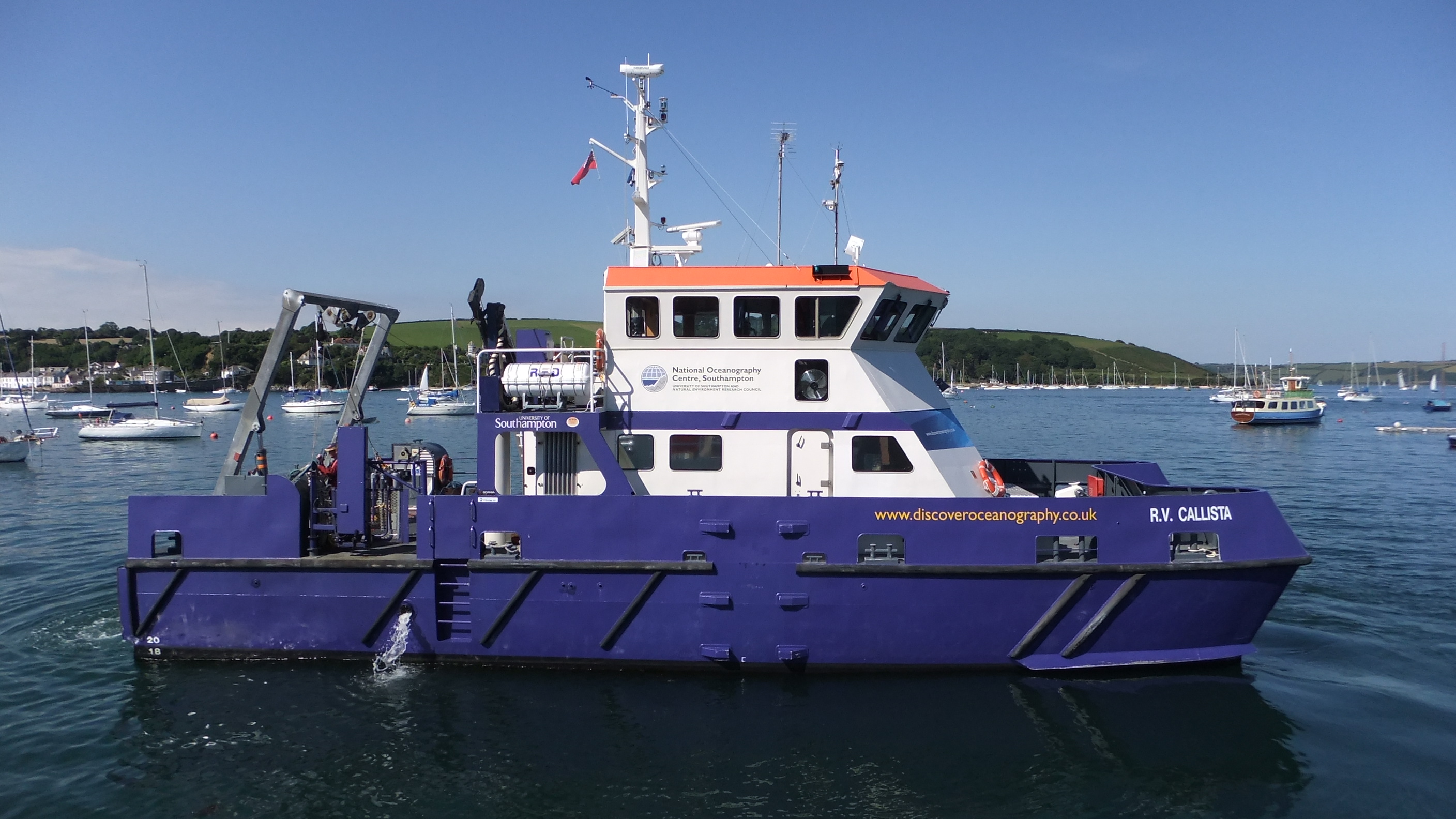
R.V.
Callista (Figure 3.1) is a twin hulled purpose built
scientific research vessel owned by the
University of Southampton. It has a large
rear deck and 3 separate deployment points
with on-board wet and dry labs enabling
chemical and physical data to be collected
and processed on the water.
Specifications:
Length:
19.75m
Breadth:
7.40m
Draft: 1.80m
Depth
Midship: 2.85m
Max Speed:
15 knots
Range: 400
Nautical Miles
Max Passengers: 30 + 4 crew
Equipment:
1 ‘A’ frame
with 4 tonne winch at stern.
2 Side
mounted Davits with 100kg capacity hand
winch.
1 Capstan 1.5 tonne pull
|
R.V. Bill Conway (Figure 3.2) is a small purpose built scientific
vessel owned by the University of Southampton. In
the cabin there is a small lab bench and a covered
area of the rear deck where data processing can take
place.
Specifications:
Length:
11.74m
Breadth: 3.96m
Draft: 1.30m
Depth Midship: 2.85m
Max
Speed: 10 knots
Range: 150 Nautical Miles
Max
Passengers: 12 + 2 crew
Equipment:
1 ‘A’ frame with
750kg winch.
2
Davits with 50kg capacity
|
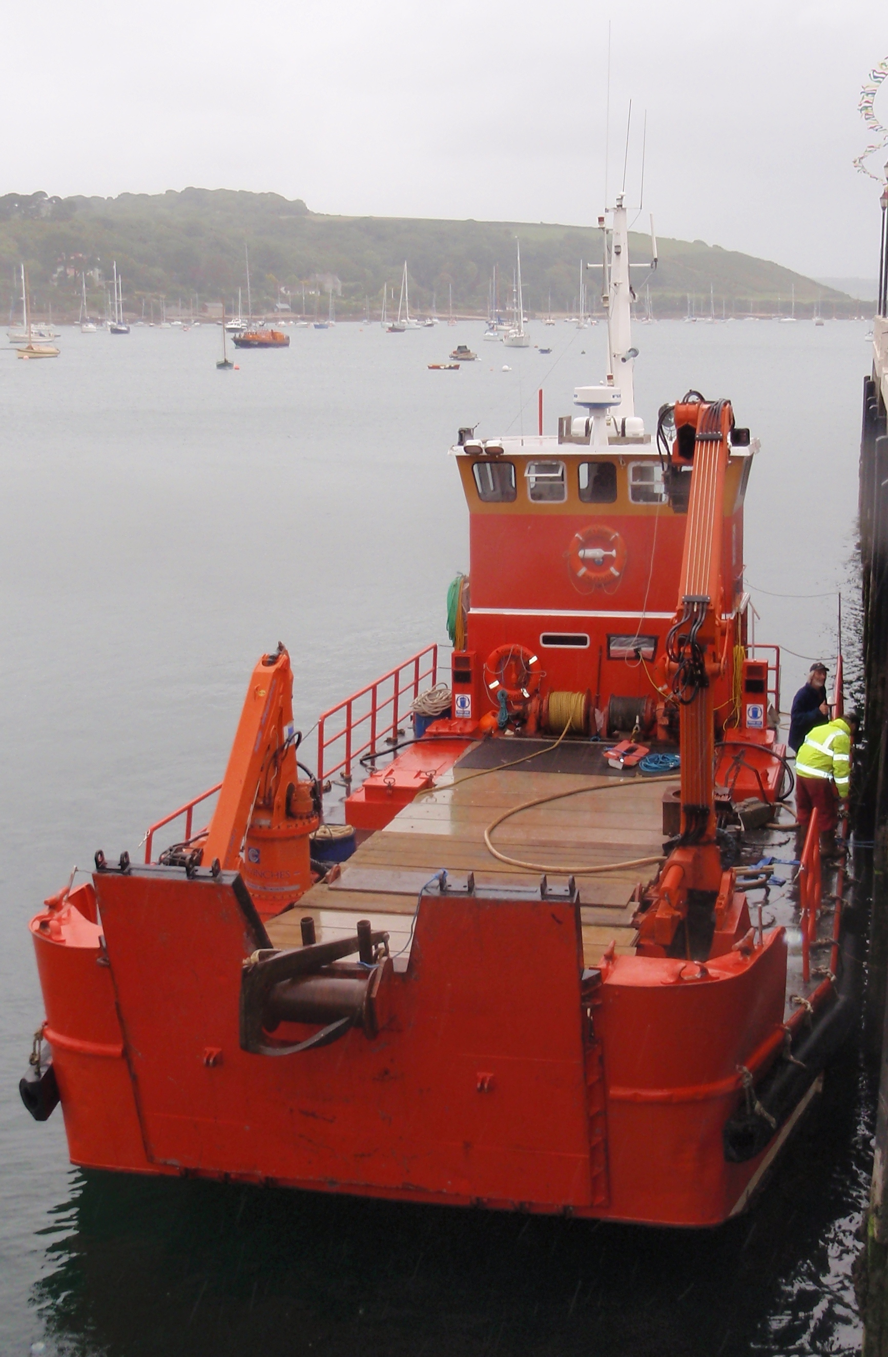
Grey Bear (Figure
3.3) is a
multipurpose, shallow draft vessel owned by FD
Marine Ltd. With its very large deck area it is
primarily used as a landing craft vessel. It is
able to go into shallower waters than most vessels
and so is highly suited for water front construction
projects, cable laying, salvage work and surveying.
Specifications:
Length: 15m
Breadth: 6.1m
Draft: 1.14m
Max Speed: 7.5 knots
Max
Passengers: 12 + 2 crew
Equipment:
1
port side Hiab 1250 crane fitted with a 2.5 tonne
winch.
1
starboard side HS Marine AK10 crane fitted with a
1.25 tonne winch.
1
stern side 3 tonne winch with roller.
2 Deck winches with 5 tonne capacity |
|
CTD |
FLUOROMETER |
TRANSMISSOMETER |
ADCP |
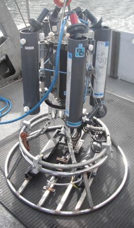
Figure 3.4 |
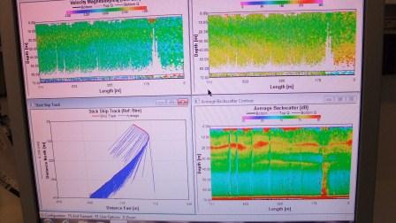
Figure 3.5 |
The CTD (Figure
3.4) is deployed from the
deck and measures
three vital physical parameters; conductivity,
temperature and depth. Salinity is then derived from
the known relationships of pressure, temperature and conductivity. Other parameters may also be measured by
instruments attached to the CTD, and sampling
bottles may be attached using a rosette system.
The CTD is attached to
the vessel by a conducting cable and data are
electronically uploaded to the vessel in situ
allowing scientists to sample based on data. |
A fluorometer was deployed on
the CTD rosette system. It emits light of a certain wavelength and
records the amount of light returned as a result of
fluorescence. It is therefore used to measure chlorophyll as
light excites the fluorophores. The data can then be used as an indication of the
phytoplankton biomass. |
A
transmissometer probe measures the amount of
suspended or particulate matter in the water column by the measurement of
attenuation of a laser beam (usually 660nm) through
a known volume. This provides a measurement of
turbidity in NTU. |
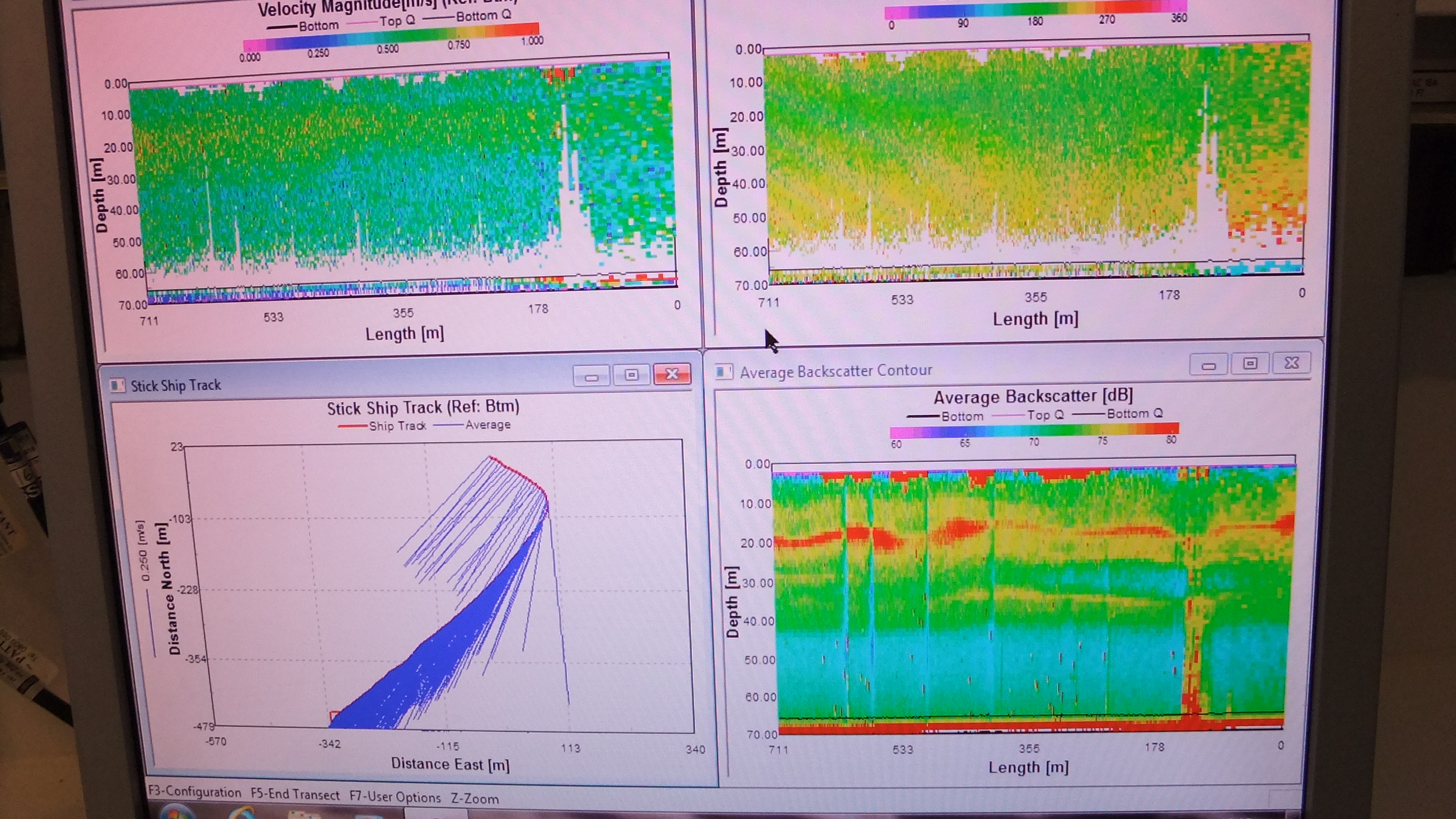
The Acoustic
Doppler Current Profilers aboard Bill Conway and Callista measure
the current speeds throughout the water column below the vessel.
An ADCP uses 3 or 4 sonar beams to measure any
non-perpendicular current. The acoustic Doppler
shift reflected by the sediment is removed from the
Doppler water shift to give an accurate reading of
current speed and direction. The ADCP also provides
an insitu measurement of the backscatter which can
be used to identify structure in the water column
and provides an indication of zooplankton
populations. The output data from the ADCP is
displayed on a screen as shown in
Figure 3.5. |
|
SECCHI
DISK |
NISKIN
BOTTLES |
HORIZONTAL
NISKIN BOTTLE |
YSI PROBE |
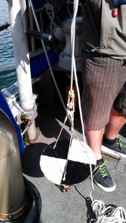
Figure 3.6 |
.jpg)
Figure 3.7 |
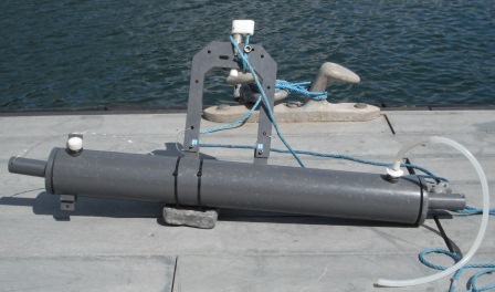
Figure 3.8 |
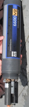
Figure 3.9 |
|
A Secchi disk (Figure
3.6) is used to
calculate the approximate depth of the euphotic
zone. The disk is circular with black and
white segments. It is lowered through the water
column at 1 metre intervals, until the disk can no
longer be seen - this is known as the Secchi depth. The
depth of the euphotic zone is calculated as 3 times
the Secchi depth. |
Water sampling
bottles such as the Niskin bottle (Figure
3.7) are deployed on a rosette
(often in conjunction with a CTD) and are used to
collect samples at a range of depths. The bottles
are deployed open so water can flow through them
reducing contamination such as biofilms and
ensuring an accurate representation of the water
column. |
A horizontal Niskin bottle (Figure
3.8) was
used for collecting water samples on the pontoon in
the Fal Estuary. It has a unique end stopper release
mechanism which allows the sampling bottle to be
used in a horizontal position.
|
A multiprobe (Figure
3.9)
measures a range of parameters including salinity, temperature (oC)
and depth (m). It may also possess probes that
measure pH, turbidity (NTU) and chlorophyll (mg g-1).
Readings are electronically transported from depth
through a conducting cable to the vessel's data
systems or
to a hand held logger. |
|
CLOSING NET |
VAN VEEN GRAB |
SIDE SCAN TOW FISH |
VIDEO CAMERA |

Figure 3.10 |

Figure 3.11 |
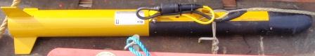
Figure 3.12 |
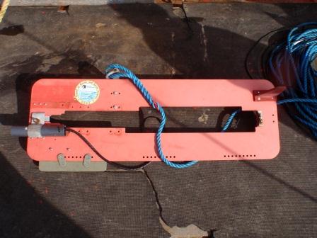
Figure 3.13 |
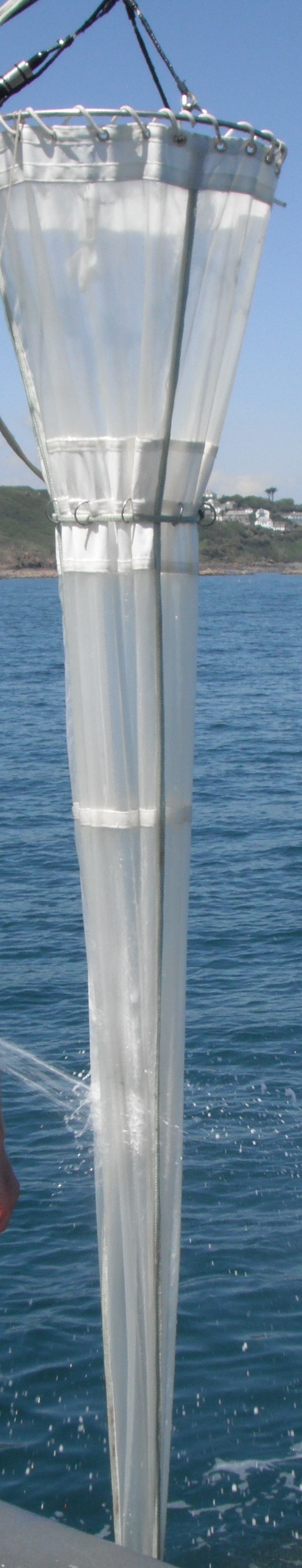
| A closing
net (Figure 3.10) allows specific sampling between two defined
depths. It is made up of a 200µm
mesh with a screw
on a vented collecting bottle. A weight keeps
the net vertical in the water column. After hauling
the net from the lower to the upper depth the
messenger weight is used to trip catch the primary
haul lines which transfer the load to a draw string
causing the closure of the net. This prevents
contamination of the sample during the recovery to
the surface. |
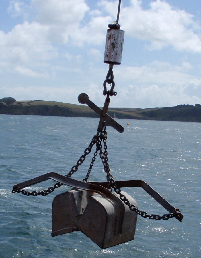
The Van Veen grab (Figure
3.11) is designed to take large sediment
samples and associated biota from areas of soft
sediment. The grab itself consists of two stainless
steel, weighted, sharp edged scoops positioned to
act like jaws. On the top of the scoops there are 4
lids which when opened allow subsampling of the
undisturbed sample in order to view stratification
of the sediment
of the sediment in its original setup before the
grab is emptied and the sediment mixes. |
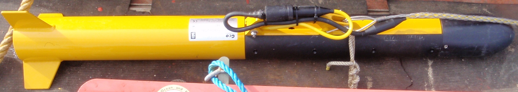
The Towfish (Figure
3.12) is the housing for the side scan sonar
transducer, which is towed through the water behind
the vessel. By towing the transducer the sonic wave
emissions can be emitted closer to the seafloor.
When the emitted acoustic signal reaches the
seafloor it is reflected back to the Towfish where
it is received, the time elapsed between emission
and reception of the signal allows for the
determination of the depth,
the images created using the
sonar are based upon the reflectivity of the
sediments, as different forms of material provide
different ranges of reflection. |
An underwater camera (Figure
3.13) allows a glimpse of the
seafloor through optical imaging. Deployed from the
vessel over the side, the camera provides real time
images of the seabed; this allows us to view the
ecosystem change beneath the boat. Submersible video
cameras are usually attached to an object that can
be controlled from the boat, and also a cable that
is attached to a small monitor. |
|
SIEVES |
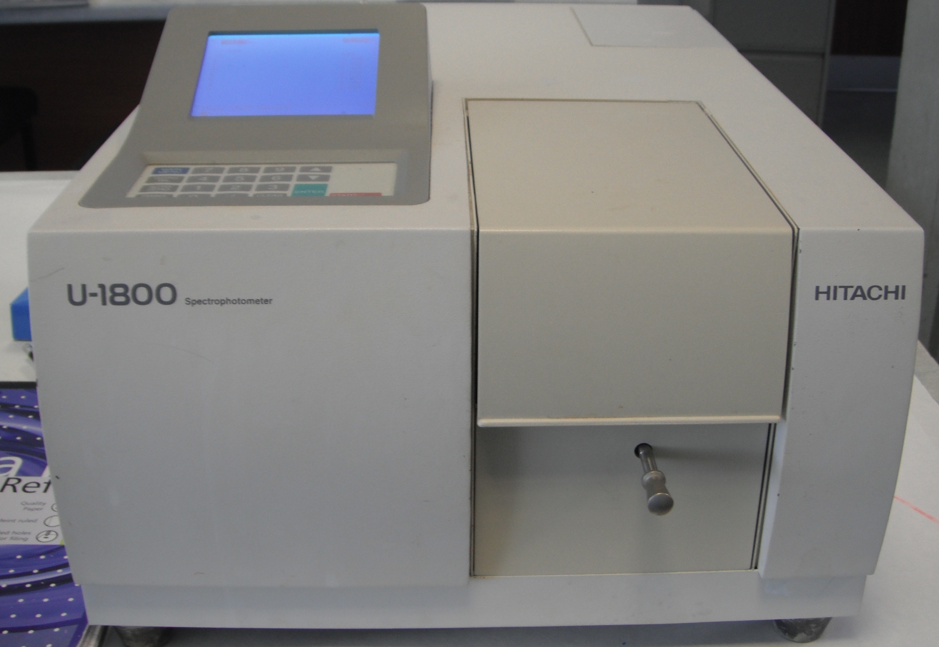
SPECTROPHOTOMETER |
WINKLER APPARATUS |
|

Figure 3.14 |
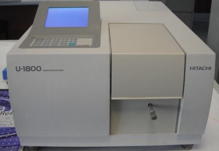
Figure 3.15 |
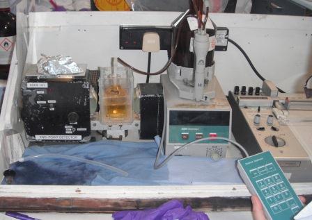
Figure 3.16 |
|
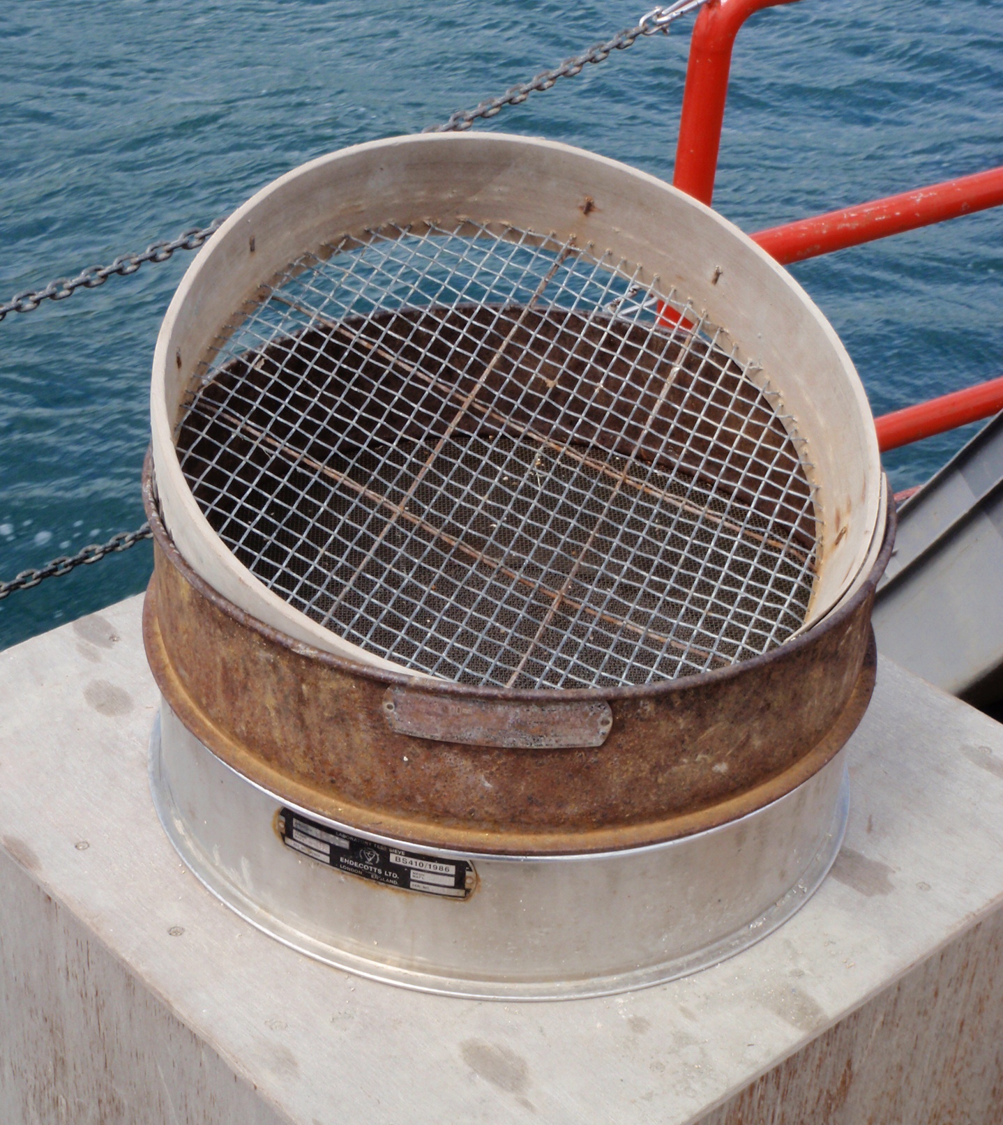
Sieves (Figure 3.14) are used to separate samples by their size.
From course to fine grained material, the size of
the mesh is used to class what is caught at that
sieves size.
|
A spectrophotometer (Figure
3.15) consists of two instruments, a
spectrometer to produce light of any selected
wavelength and a photometer to measure the intensity
of light. The instrument is arranged to allow a cuvette of a liquid sample to be placed between the
spectrometer beam and the photometer. The light from
the spectrometer as it passes through the cuvette is
measured by the photometer, which is shown on the
screen. The signal on the screen changes as the
amount of light absorbed by the liquid changes.
|
The winkler apparatus (Figure
3.16) is used to measure the
concentration of dissolved oxygen. This is done by
titration; sodium thiosulphate is added
to the sample in the bottle until the solution
becomes clear. |
|
Lab Methods
      |
Phosphate
|
|
1.
1. Preparation of phosphate working
standard The standard
must be
freshly prepared. The stock solution was diluted 400 fold
by taking 1ml and made up to 100ml with MQ
water in a volumetric flask. Then 25ml was
separated and
made up to 100ml with MQ water, giving a
solution containing 15µmol per litre which is used
to prepare the calibration standards.
2. 2.
Preparation of Calibration and Blank
solutions Using a 5ml hand pipette, 10ml of MQ
water was carefully added to three tubes labelled as
blanks. Using appropriate pipettes, 50µl, 100µl, 200µl,
500µl, 1000µl and 2000µl was added each to 3
separate sample tubes, giving 21 test tubes. All
tubes were made up
to 10ml using MQ water. These tubes were treated the same as the sample tubes and
then the analytical methods below were followed. These calibration tubes will
have the following phosphate concentrations as in
Table 4.1.
|
Addition volume (µl) |
50 |
100 |
200 |
500 |
1000 |
2000 |
|
Phosphate conc. (µmol l-1) |
0.07 |
0.15 |
0.3 |
0.75 |
1.5 |
3.0 |
Table 4.1
Fresh mixed reagent was
prepared by combining 20ml
Ammonium Molybolate, 50ml Sulphuric Acid (2.5M), 20ml Ascorbic Acid, 10ml Potassium antimonyl tartrate
producing 100ml total. 1ml mixed reagent was added to every
sample tube (blanks, calibration tubes and samples
alike) then mixed well and left for 1 hour.
Then the spectrophotometer set at 840nm was used to determine
the
absorbance of each sample, calibration and blank
tube. The calibration and blank tubes are used to
calculated the phosphate concentration of the sample
tubes based on the measured absorbencies. |
Silicate
|
|
The laboratory analysis to determine the amount of
silicon present in each sample was carried out as in
Mullin & Riley (1955); a slight modification was that
the river end member samples were diluted by a
factor of 5. A sub-set of standard samples were used
to perform a calibration using silicon solutions of
known concentrations, which were also placed into
the spectrophotometer and their absorbencies measured.
1. Standard preparation A
stock silicon solution of 35.6mmol l-1
was diluted using a 25 times dilution to create the
working standard solution.
Further dilution was then
carried out to create the following standards:
1.4μmol l-1 , 2.8μmol l-1 ,
7.1μmol l-1 , 14.2μmol l-1,
21.4μmol l-1.
2. Sample preparation
2ml of molybdate reagent was added to 5ml of each
silicon sample and left to stand for 10 minutes. 2ml
of molybdate was also added to 5ml of MQ water to be
used as blanks. A
mixed reducing agent (MRR) was prepared by mixing
metol sulphite, oxalic acid, sulphuric acid and MQ
water. 3ml of the MRR was added to all samples,
standards and blanks, and left to stand for 2hours. The absorbance of the samples were measured on a
spectrophotometer (U1800) at a wavelength of 810nm,
a 4cm cell was used. |
Dissolved Oxygen - Winkler Titration
|
|
Glass bottles are used for
dissolved oxygen measurements in order to prevent
contamination. Samples were taken from Niskin bottles
before any other samples were taken to avoid
contamination, and
were siphoned through rubber tubing with a tight seal
on the valve. Air bubbles were removed from the
tubing and the glass bottles were filled to a third and
rinsed then emptied to clean which avoids
contamination. The bottles
were then filled to overflowing to avoid
trapping any air within the bottle. Winkler
reagents were added to the sample; 1ml manganous chloride and 1ml
alkaline
iodide solution using a pipette. This fixes the
oxygen in the bottles, which are then stored in water to
prevent leaching from air through the stopper until
lab analysis.
In the lab, 1-2ml of sulphuric
acid 10M was added to and mixed in each bottle to
release the oxygen, turning the solution to a clear
yellow. The bottles were placed into the end point
detector and sodium thiosulphate (normality 0.22)
was
added using a metrohm device until the solution
began to clear. Further additions were monitored on
the Servoscribe 1s until the needle ceased movement
and plateaued. The metrohm reading was recorded. As
the amount of sodium thiosulphate added to the
sample was known, the dissolved oxygen concentration
could therefore be calculated. |
Chlorophyll
|
|
Chlorophyll a concentration is currently the best
index for estimating phytoplankton biomass (Huot et
al., 2007) although the fluorometry readings
obtained in the fieldcourse did not correlate very
well to the CTD fluorometer readings; the CTD
readings should be assumed to be the more accurate
reflection of chlorophyll. In order to chemically
analyse water samples for chlorophyll however, seawater was filtered into
glass and plastic bottles for oxygen and nutrient
analysis respectively on the boat. The porous glass fibre
filters that the water was filtered through was then
stored in 90% acetone; the acetone acts as a solvent
and extracts the chlorophyll. The test
tubes were frozen overnight. Using a fluorometer in
the laboratory the following day, the fluorescent
properties of the chlorophyll pigment in the acetone
were measured and determine the amount
of chlorophyll present using the following equation:
Chlorophyll (µg l-1) = ( Volume acetone / Volume
seawater filtrate ) * Fluorometer Reading
As there were two filters for each water sample
taken, the results gained in the lab could be
compared to give a reasonable indication of the
chlorophyll levels in the sample generally.
|
Zooplankton
|
|
Formalin was initially added to
each 500ml zooplankton sample bottle in order to preserve the
zooplankton. In the laboratory after mixing the
sample by
simply inverting the bottles, 10ml of the sample was pipetted into a measuring cylinder. Then 5ml of
this sub-sample was pipetted into a Borgorov chamber
and viewed under a light microscope, and each zooplankton was identified with the aid of photo
guide books. The individual organisms were tallied
into a table under the major taxa groups found in
the area: Copepoda, Copepoda Nauplii, Cladocera,
Mysidacea, Chaetognatha, Hydromedusae, Siphonophorae,
Ctenophora, Appendicularia, Decopoda, Cirripedia, Polychaeta, Gastropod, Echinoderm and
fish larvae.
|
Phytoplankton
|
|
Water samples were added to
bottles containing Lugols solution which preserved
the phytoplankton. 100ml of solution was then left
in a settling column overnight to allow the
phytoplankton to settle. In the laboratory the top 90ml of each
sample was removed with a vacuum pump to leave a
concentrated sample. From this 10ml sample a
smaller subsample of 1ml was taken and added to a
Sedgewick-Rafter Counting Chamber which was placed
under an optical microscope to be viewed. 5 vertical transects of
20 1μl squares
were viewed with the number of cells in each square
being recorded and the different species were
identified and logged. |
|
| |
| |
Estuarine        |
|
Introduction
Physical, chemical and biological data were
collected in the Fal Estuary (Figure
5.1) in order to establish an understanding
of how the Fal Estuary behaves. As an estuary, the area is a transition
zone between the freshwater input of the rivers into the estuary and
the coastal sea, and therefore can be expected to have differing
characteristics to the coastal sea observed in the offshore
practical. The Fal Estuary is a high nutrient region subject to
various pollution pressures.
Physical data provide an indication of the
physical structure of the Fal Estuary and provide information on
whether the estuary is mixed, partially mixed or stratified. The
data collected throughout the estuary will provide an overview of
how the physical structure changes throughout the estuary and enable examination
of how the tides affect the conditions in the estuary. The
chemical data collected will give an indication of the behaviour of
nutrients in the estuary. Studying the biological characteristics in
conjunction with the rest of the data will be used to indicate what
is controlling or limiting the phytoplankton in the estuary.
The data can be compared to data collected in the offshore
practical.
Data on the estuary were collected in two ways
in order to determine how the physical, chemical and biological
characteristics of the estuary vary temporally and spatially. Lagrangian
measurements were collected using the
R.V.
Bill Conway along the Fal Estuary commencing up the estuary at
low water in the morning and travelling down the estuary throughout
the day during the flood and ebb tidal cycle. Physical data were
collected using a
CTD to measure the
temperature, salinity, turbidity and chlorophyll,
and an
ADCP system to collect data on the flow direction and velocity. Water
samples were collected via Niskin bottles mounted on a rosette. Water
samples were filtered and then used in the laboratory to determine the concentrations of
phosphate, silicon, dissolved oxygen and chlorophyll as outlined in
the lab techniques section. Phytoplankton samples were also
collected from the Niskin bottles. Zooplankton was collected using a
210 micron net and towed for 5 minutes at selected stations. A
Secchi
Disk was used to estimate the depth of the euphotic zone
and is used in conjunction with the transmissometer on the
CTD which
indicates the light attenuation of the water column.
Eulerian measurements were taken at the King
Harry pontoon, using an YSI multiprobe to measure the salinity
temperature, chlorophyll, turbidity and pH through vertical profile
at a fixed point on the estuary. A
Niskin bottle was also used
at the surface to measure the same biological properties as aboard
the R.V. Bill Conway. The data from the pontoon
were used to observe the changes in the properties over time and the tidal
cycle.
The data
were collected in conjunction with Group 11: Group 6 collected boat
data in the morning, whilst group 11 were on the pontoon. Group 6 then took over measurements at the
pontoon at 12:00 GMT whilst group 11 continued collecting data on the
boat further down the estuary. Ancillary data for the survey can be
found in Tables 5.1 and 5.2.
| Date |
29/6/2011 |
| General Weather |
Sunny with some
cloud cover |
| Visibility |
Good, clear day |
| Sea State |
Very calm |
| Cloud Cover |
3/8 in the morning to 2/8 in
the afternoon |
Table 5.1
| 29/6/2011 |
Tide Times GMT |
Tidal Height
(m) |
| Low Water |
0952 |
1.5 |
| High Water |
1548 |
4.8 |
| Low Water |
2221 |
1.5 |
Table 5.2 |
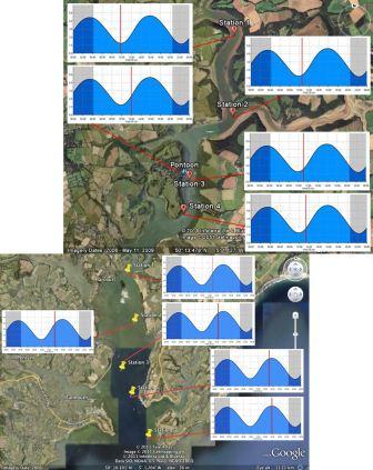
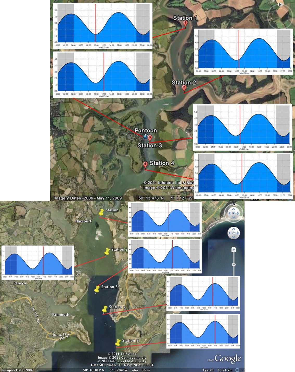
Figure 5.1 |
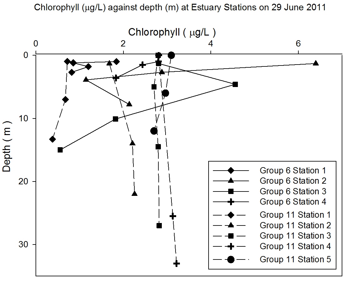
Physical Characteristics
The
sampled area of the Fal estuary is well mixed. The
lowest salinity was sampled at 25 at the furthest point up
the estuary that could be sampled and the highest salinity
measured was 34 towards the mouth of the estuary. The top
part of the estuary sampled by group 6 had the biggest
change of salinity of 8 found mostly at the station 1 and 2;
salinity at station 3 and 4 is around 33. This compared with
the bottom of estuary sampled by group 11 having a change of
2 where surface salinity stays around 35 from stations 2-5.
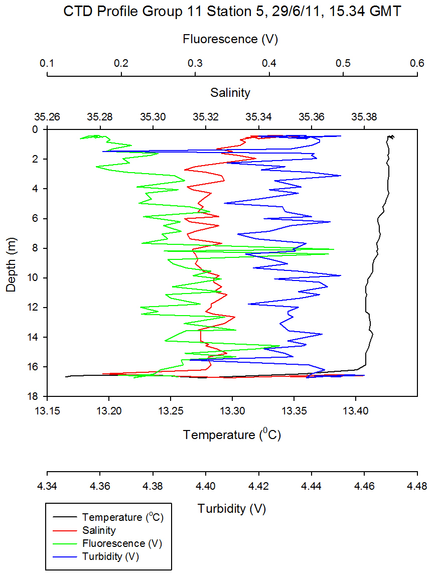
Surface
temperature down the estuary changes from 15.7°C to 13.4°C at the
last station (Figure
5.8). The top of the estuary sees little change in surface
temperature of 0.4°C whereas the bottom of the estuary shows a
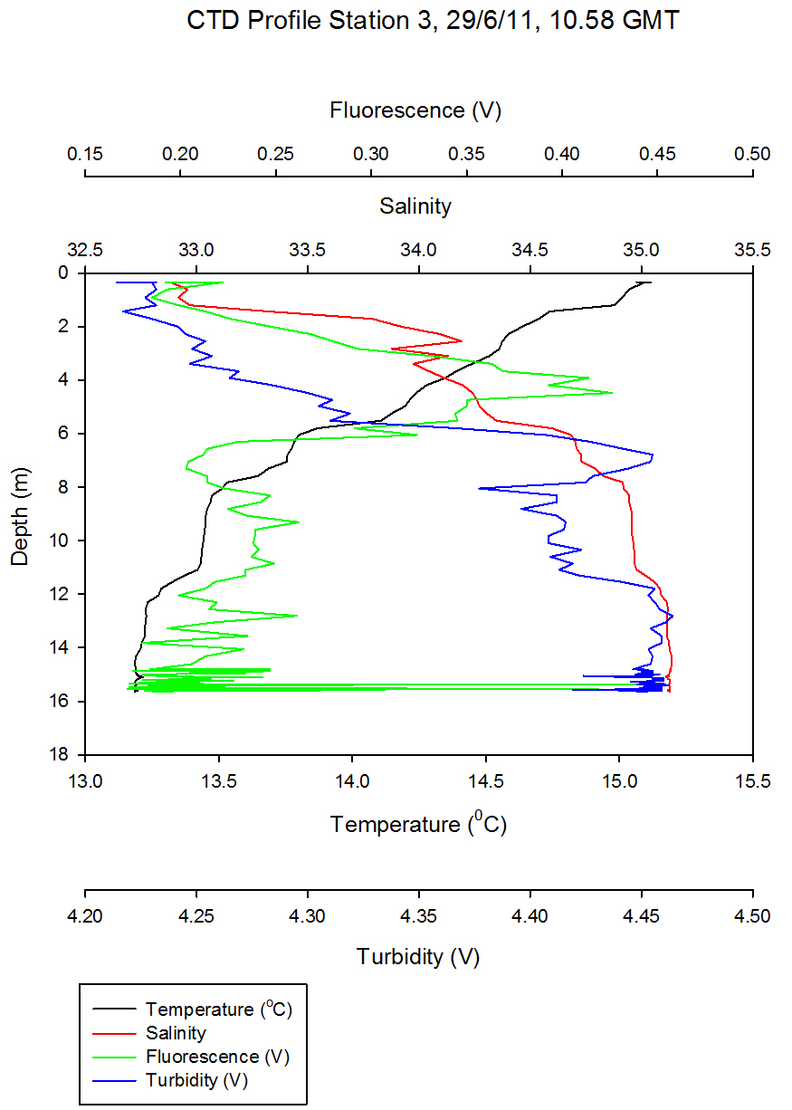
change from 13.7 to 13.4°C. The largest change in temperature change is
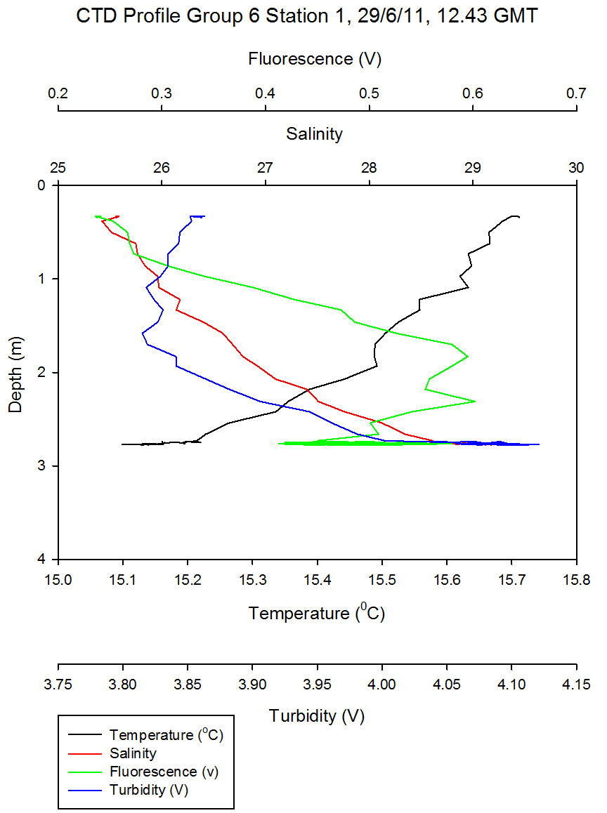
at group 6 station 3 (Figure
5.7) where in 8 meters the temperature goes from
15.2 to 13.5°C – this stratification could be due to intense heating
together with this region not being as well mixed. Little change in
temperature at bottom of the estuary could be due to incoming tide
going up the estuary and mixing the surface water at the lower end
of the estuary (particularly as this station was sampled at high
water).
Fluorescence, used to indicate chlorophyll levels in the estuary,
varies from surface values of 0.3 at the top of the estuary to 0.13
volts at the bottom of the estuary. Fluorescence stays relatively
low at the bottom of the estuary with the maximum value being 0.1 at
the surface. At the top of the estuary there is a peak of 0.6 volts
at station 1 (Figure 5.2) and then fluorescence stays fairly constant around 0.4
volts. This indicates that there might be higher phytoplankton populations near the top
of the estuary.
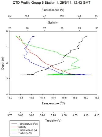
Figure 5.2 - Station 1 |
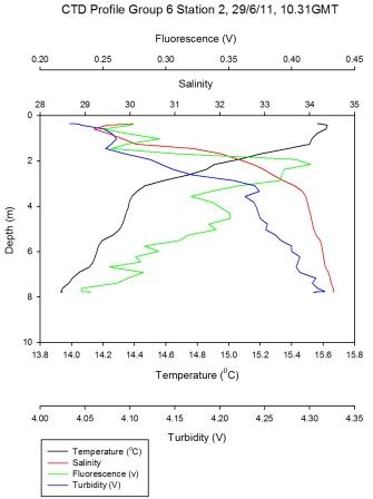
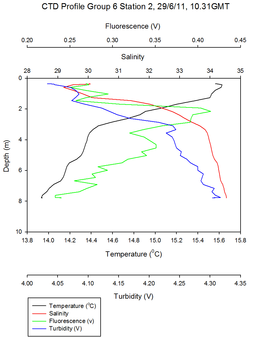
Figure 5.3 - Station 2 |
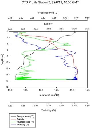
Figure 5.4 - Station 3 |
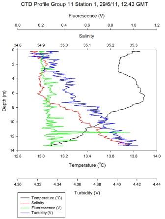
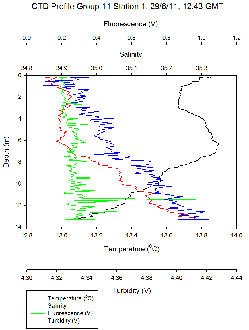
Figure 5.6 - Group 11 Station 1 |
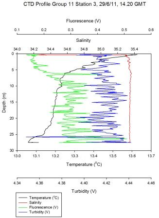
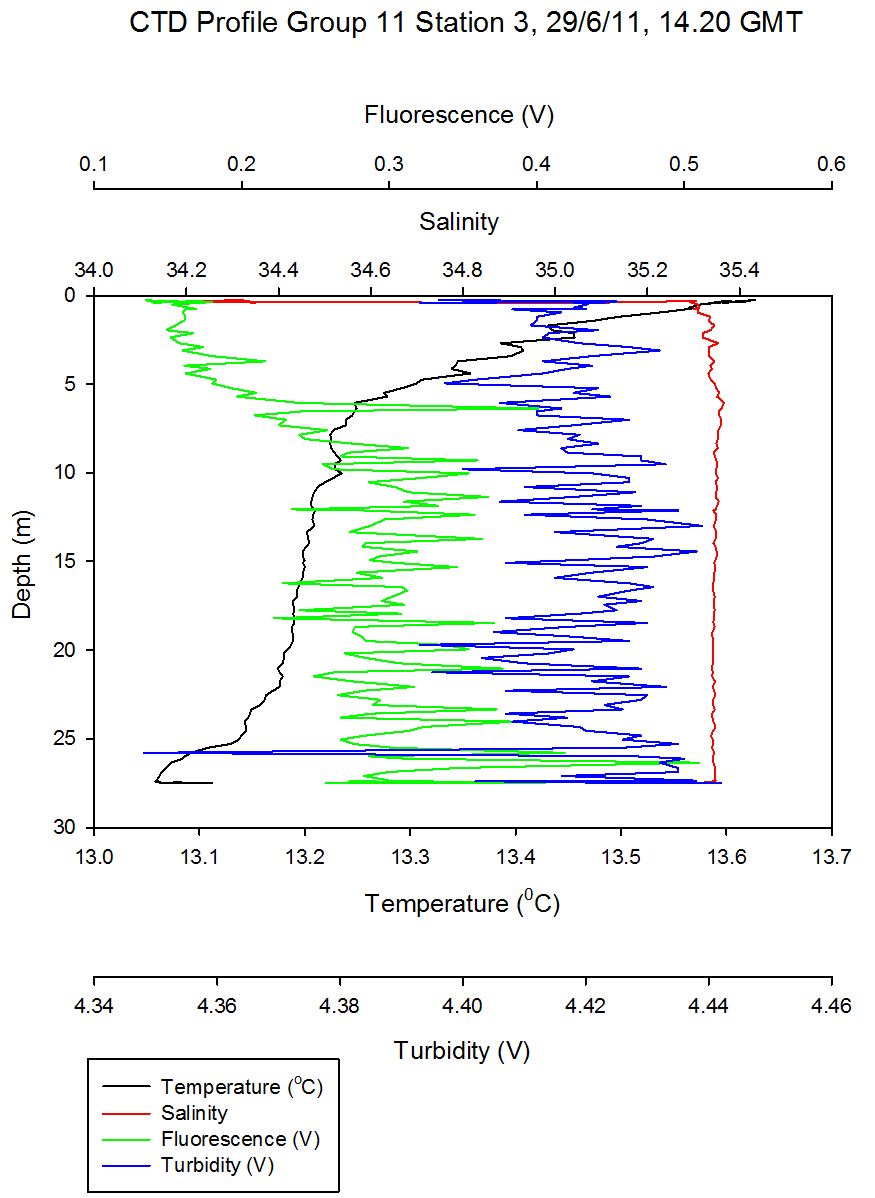
Figure 5.7 - Group 11 Station 3 |
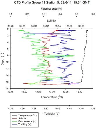
Figure 5.8 - Group 11 Station 5 |
|
Richardsons number
calculations (see offshore) of
Group 6 station 2 and Group 11 station 5 located up-estuary
and at the estuary mouth respectively are shown in (Figure
5.9). At station 2 low Ri numbers
describe turbulence throughout the water column, except at
4m where Ri=0.252. This
corresponds with the depth of the surface warmed water
boundary as seen in
Figure 5.3. On a large temporal scale, for example offshore, a
high Ri number depicting laminar flow is predictable at such
a boundary. However, stability might not be maintained at
station 2 in a tide dominated estuary such as the Fal. Here,
some gravitational stability has been reached, however shear
instability prevails over laminar flow (with Ri>1).
At Group 11
station 5 (Figure
5.8) near the mouth of the estuary there is no
synonymous warmed surface water layer and values of Ri<1/4
describe turbulent flow in the entire sampled water column.
At the time of sampling the water depth was twice as deep at
Group11 station 5 when compared to station 2. This is due to
a deeper channel and because this station survey, at 15:34
occurred 14 minutes before high water making the water
column ~3.1m higher than the low water height when station 2
was sampled. Both vertical, horizontal, wind and tidal
mixing occurs at the estuary mouth which is in close
proximity to open ocean. |
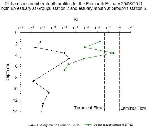
Figure 5.9 |
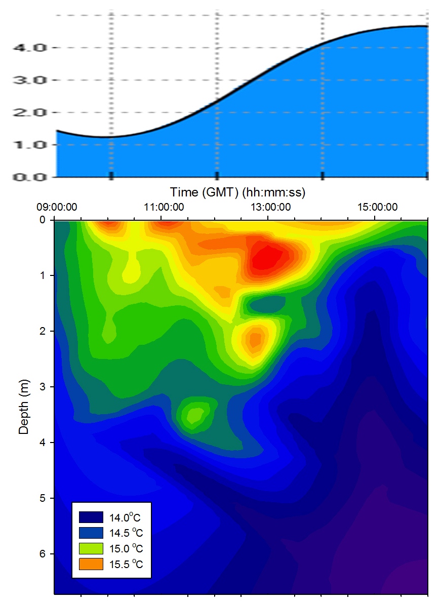
Pontoon
EAST
|
Temperature |
Solar surface warming was evident from 09:30GMT throughout the day
heating up the surface layer. The warming effect was
countered by the rising tide which drew cooler seawater up
into the estuary. From low water (09:52GMT) to the end of
sampling at 16:00GMT the influx of seawater into the estuary
cooled the deep waters and created a significant level of
stratification in the water column, limiting solar
heating to the uppermost 0.5m. As the tide rose the cool
deep seawater layer moved shallower due to the volume
of seawater being forced up the estuary displacing the
freshwater; this can be seen on the contour plot (Figure
5.10) as a region
of cooler water below 1.5m. This seawater intrusion can be
identified on the salinity contour plot (see below). At high
water (15:48GMT) the cool seawater layer dominates the water
column starting at 1.5m and extending to the bed.
|
|
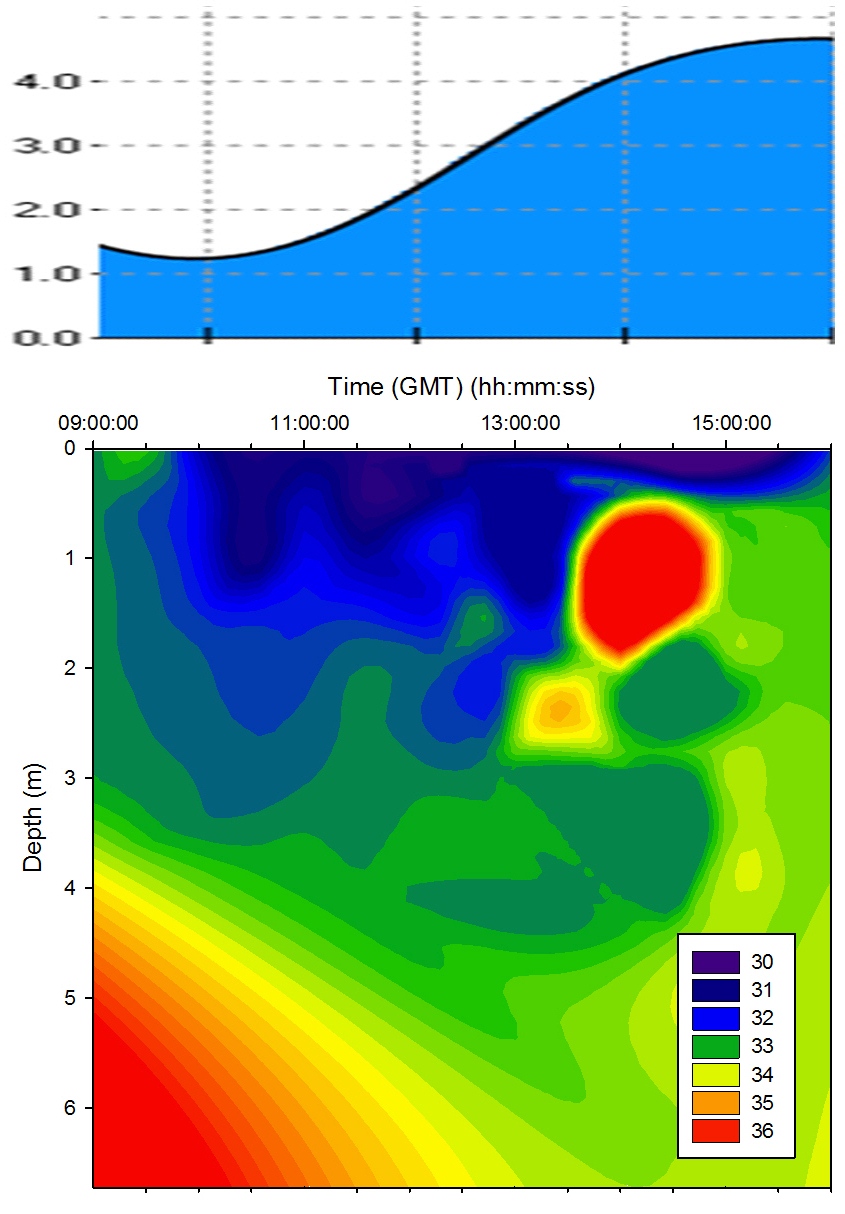
Salinity |
The temporal proximity of the morning samples to low water
resulted in a region of high salinity in water below 4m;
this is due to the tidal forcing drawing the denser seawater
back seaward from the estuary below the freshwater as the
tide fell. Salinity was lower in the surface layer
throughout the sampling time due to freshwater laying above
the denser seawater though the level of stratification
varied across the tidal cycle. At 14:30GMT a protrusion of
saline water pushed through the layer of freshwater at depth
1m. This may have been linked with weakening tidal forcing
as the tidal cycle approached high water. A salinity hotspot
is seen in
Figure 5.11 - this is due to sigmaplot extrapolation and
so ignored in analysis. |
|
Chlorophyll |
Figure
5.12 shows a high concentration of chlorophyll measured
at approximately 2m for the majority of the tidal cycle. At
13:00GMT the chlorophyll maximum moved upwards to 1m. At the end of sampling (16:00GMT) a chlorophyll maximum was measured deeper than
before below 4m. This is caused by the drawing in of
phytoplankton with the seawater as the tide rises to high
water. |
|
Turbidity |
Figure 5.13
shows that there was a high level of turbidity in the bottom water layer due to
turbulence suspending silt and detritus from the bed. The
extreme variations between measurements taken before and
after 12:00GMT may indicate the different depths of water
that group 6 and group 11 were sampling in. Group 11 were
sampling in shallower water due to the tidal cycle which
meant that more of the water column was being influenced by turbulence with the bed
and resulting resuspension of sediment. However group 6 were sampling
closer to high water when the water column was deeper and
therefore turbulence
with the seabed was less significant. |

Figure 5.10 Temperature |

Figure 5.11 Salinity |
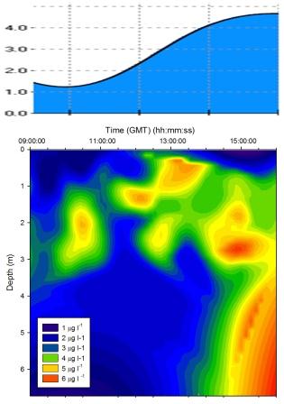
Figure 5.12 Chlorophyll
|
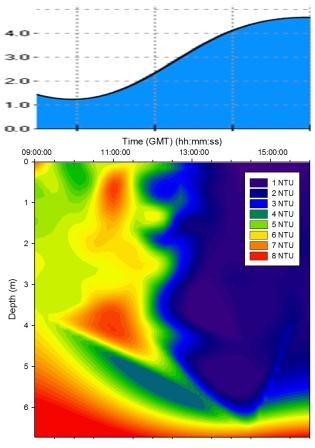
Figure 5.13 Turbidity |
WEST
|
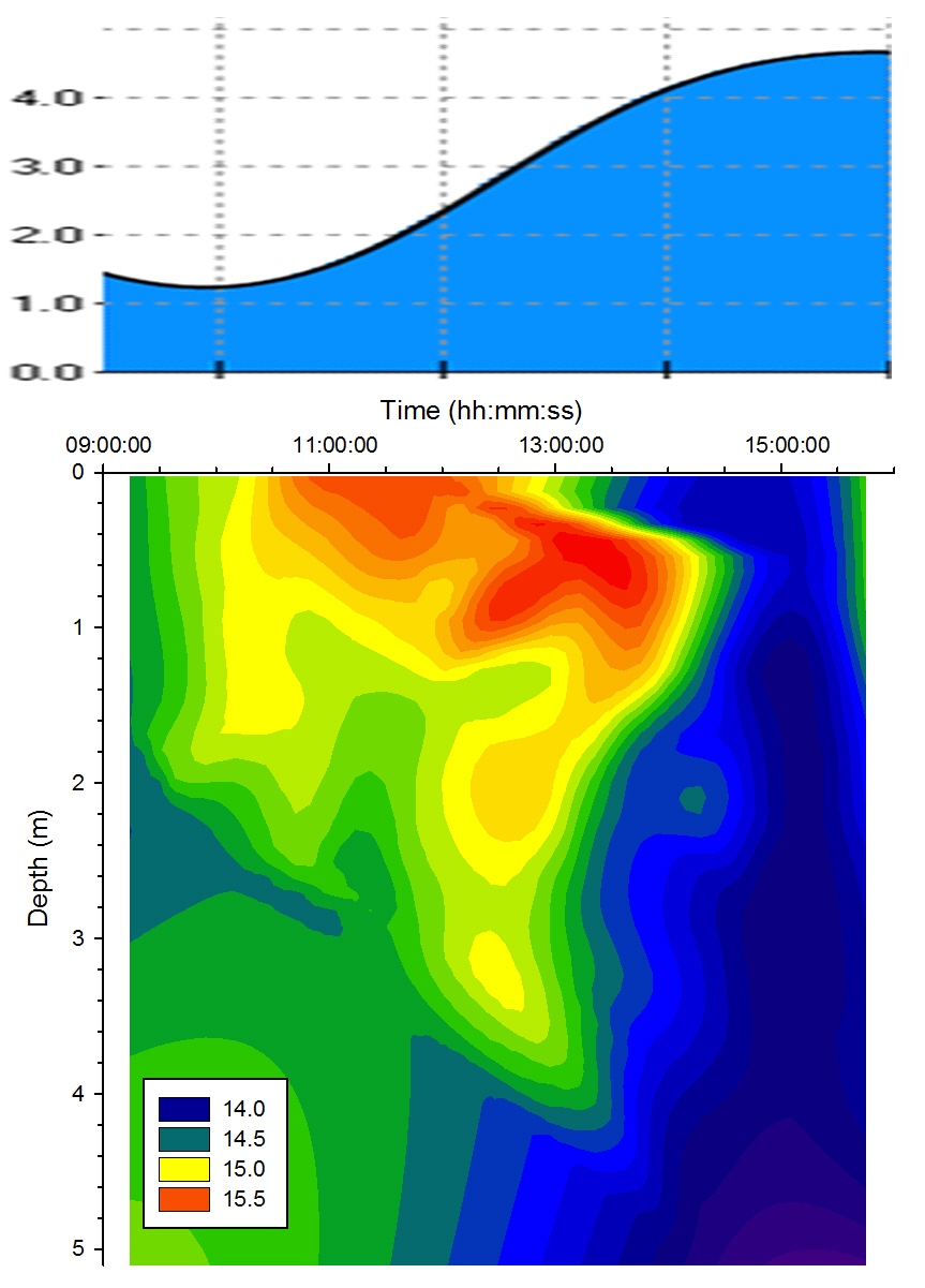
Temperature |
Figure
5.14 shows solar surface warming was evident from 09:30GMT throughout
the day heating up the surface layer. As the tide rose the
cold deep seawater layer moved progressively shallower until
at 14:00GMT it displaced the freshwater at the surface
leading to a cold surface layer existing for a short period
of approximately one hour. Simultaneously the warm
freshwater surface layers are pushed up the estuary by tidal
forcing as the tide rises. |
|
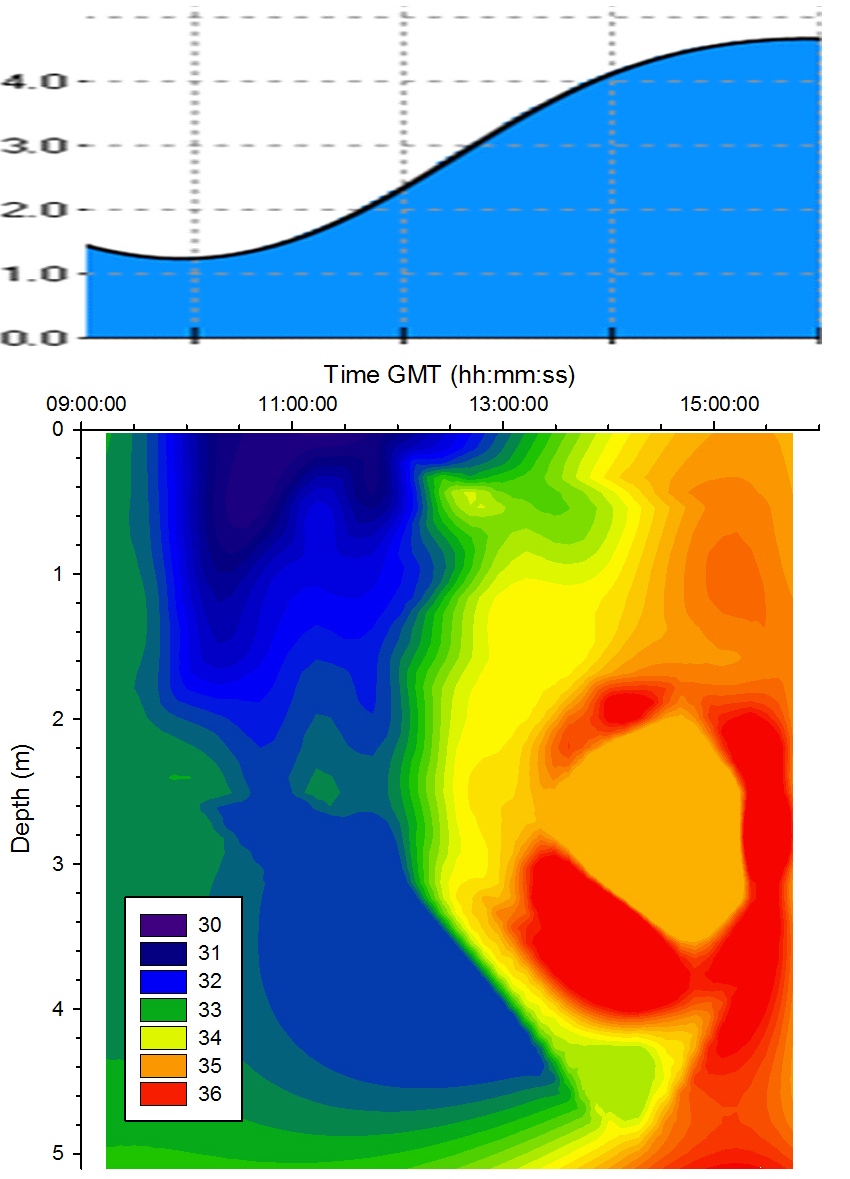
Salinity |
Figure
5.15 shows that at low water (09:52GMT) river flow was dominant and so the
salinity was low. As the tide rises tidal forcing pushes
seawater up the estuary and this can be seen on the contour
plot as a region of high salinity. There was a lag between
the turning of the tide at 09:52GMT and the rise in salinity;
this may have been due to the counteracting force of river
water coming down the estuary. |
|
Chlorophyll |
Figure
5.16 shows that chlorophyll concentrations increase at
approximately 1m throughout the period of sampling. A
maximum was measured at 2.5m and below from 09:00GMT till
13:00GMT. This was caused by the falling tide in the first
52 minutes of sampling pulling chlorophyll rich water down
from upstream. A second maximum was observed
at 14:00GMT where tidal forcing pushed chlorophyll rich
seawater up the estuary beneath the freshwater. |
|
Turbidity |
Figure
5.17 shows similar
trends were observed as on the east side of the pontoon for
turbidity. |
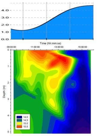
Figure 5.14 Temperature |
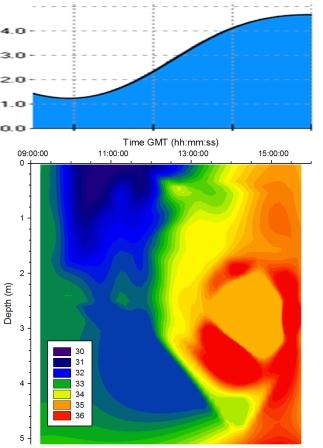
Figure 5.15 Salinity |
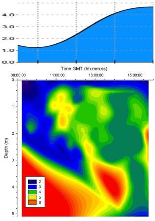
Figure 5.16 Chlorophyll |
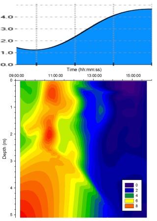
Figure 5.17 Turbidity |
|
Variation in East and West measurements from the pontoon
The
measurements taken using the YSI probe on the East and West
side of the pontoon show variations in data collected,
despite their close spatial proximity. It is important to
analyse the differences between these two sites before any
assumptions are made about the relationship between
measurements made on the pontoon and on RV Bill Conway.
Variations on this small spatial scale can be used to assess
the significance of variations seen between stations sampled
on RV Bill Conway. The East and West sides of the pontoon
experience differing levels of disturbance from passing
vessels: the East side of the pontoon being disturbed and
mixed by ferries every 15 minutes or so whereas the West
lies relatively undisturbed which may have lead to the
stabilisation of water layers that were unable to develop on
the East side. The two sides may have been affected in
different ways by tidal forcing due to the interruption of
the tidal flow by the pontoon structure. There was also the
issue of depth; the West side of the pontoon was
approximately 2m shallower than the East side so the
development of layers in the column would be affected.
|
Light Analysis
|
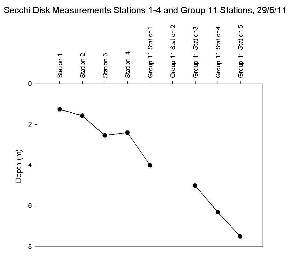
The Secchi disk measurements
(Figure 5.18)
show a clear trend between the upper sampling stations and the lower stations. The
shallowest Secchi
depth was measured at station 1 with a depth of 1.26m and the
deepest at Group 11’s station 5 with a depth of 7.5m which partly
reflects the deepening of the natural river channel and
hence the varying proximity of the euphotic zone to the sediment of
the seabed. Group 11's station 5 was sampled 14 minutes
before high water therefore the Secchi depth is deeper due
to reduced bottom turbidity, as highlighted by the pontoon
time series. There is a very slight decline in depth between
station 3 and 4 of 0.1m but all other measurements show an increasing trend which reflects a
larger euphotic zone (recognised as approximately three
times the Secchi disk depth unless this exceeds the depth of
the bed).
The
attenuation coefficient, k, is an indication of
the rate at which light is absorbed within the water column. The
highest k value and therefore fastest attenuation rate is shown at
station 1 with a value of 1.14 (Table 5.3). There is then a general decline down
the estuary towards the mouth, with the lowest value at group 11 station 5 with a
k value of 0.19 indicating a deeper euphotic zone.
| Station Number |
Secchi Depth (m) |
k
- Attenuation Coefficient |
|
Station 1 |
1.26 |
1.14 |
|
Station 2 |
1.57 |
0.92 |
|
Station 3 |
2.54 |
0.57 |
|
Station 4 |
2.40 |
0.60 |
|
Group 11, Station 1 |
4.00 |
0.36 |
|
Group 11, Station 2 |
No Data |
|
Group 11, Station 3 |
5.00 |
0.29 |
|
Group 11, Station 4 |
6.30 |
0.23 |
|
Group 11, Station 5 |
7.50 |
0.19 |
Table 5.3 |
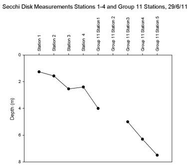
Figure 5.18
|
Phosphate Analysis
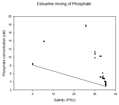
Figure 5.19 |
The mixing diagram is
a diagram which shows
the concentration of a solute against an index of
conservative mixing in the estuary - salinity is
commonly used. The diagram can be used to
understand the behaviour of solutes, in
this case phosphate, as they flow through the
estuary.
The four assumptions for
estuarine mixing diagrams were met: the constituents
were assumed to be at steady state, the end member
concentrations are constant on a timescale somewhat
greater than the residence time of the estuary,
there is only one riverine and one end member and
there were no additions of pore waters.
Samples taken at stations up the estuary
were taken over a relatively narrow salinity range
as this was the extent of the estuary that could be
surveyed in the R.V. Bill Conway; the low number of riverine inputs mean that the estuary is relatively
saline for quite some distance up the estuary.
Freshwater riverine end members were obtained by
staff members separately.
The theoretical dilution line
in the graph (Figure
5.19) between the riverine and saline end
members represents the conservative behaviour
of solutes - changes in concentration are solely
due to mixing. If there is deviation of the data
points away from the TDL addition or
removal of the solute is indicated. The graph shows that there is a
dramatic increase above the TDL. This demonstrates that
phosphate is behaving non-conservatively and is
being added to the water column. This could be a
result of possible anthropogenic factors such as
sewerage outfalls and agricultural inputs further up the estuary.
A
mussel farm near King Harry pontoon may
also cause a change in levels of dissolved phosphate
in the water column.
Mussels
have been farmed near the King Harry Pontoon and
close to station 3 by West Country Mussels of
Falmouth since 1993 (accessed:
www.westcountrymussels.co.uk, 7th
July 2011).
An
example of an input of phosphate in the Fal Estuary
is a survey of the mussel farm by Envirogene which
used DNA to establish that there was persistent
contamination of the waters by human and bovine
faeces (there are a large number of cattle/dairy
farms in the area). In addition significant inputs
of human faecal matter were detected entering the
Fal at the King Harry Ferry.
(accessed:
www.envirogene.co.uk/downloads/casestudies/envirogene_case_fal.pdf
, 7th July 2011). |
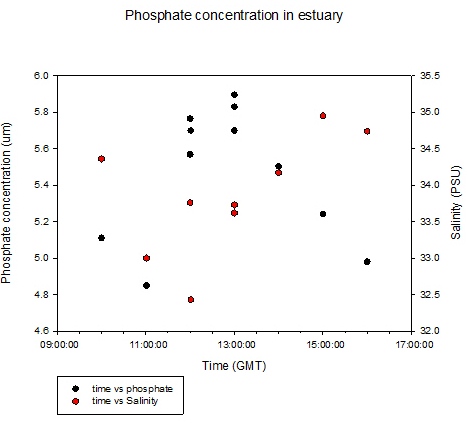
Figure 5.20 |
Phosphate Time
Series at King Harry Pontoon
Low tide was at 09:52GMT and salinity
was at its lowest following this because the influence of salt
water was lowest at low tide, although a small tidal
lag was observed. With the flood tide, the salinity
began to increase again with a peak around high tide
(Figure 5.20).
Phosphate concentration
increased from low tide reaching a peak at
13:00GMT of 5.9µm. From low tide to high tide the
increase in phosphate could be due to nutrient
inputs further downstream being washed up the river.
Nutrient inputs could be due run off from
agricultural practices in the region and sewage
treatment farms. Phosphate in the Fal Estuary is
also known to be discharged from mine drainage
sites, notably in the Carnon Valley.
|
Dissolved Silicon Analysis
Estuary
|
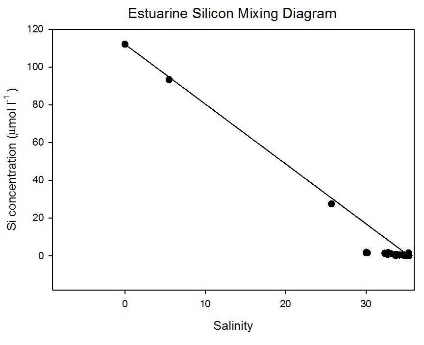
The estuarine mixing diagram (Figure
5.21) shows
that dissolved silicon was behaving conservatively between
the salinity 0 and 25; this suggests that the extent of
mixing between these two points was the determining factor
for the concentration of dissolved silicon at this time. This observed
conservative behaviour does not guarantee that no biological
uptake was occurring; there could have been a low rate of
uptake which was not observable as non- conservative
behaviour. This slow removal could be due to turbidity
caused by the heavy rainfall during June 2011, this could
affect the growth of diatoms; such effects have been shown
in the River Zaire (Cadee 1978).
Another suggestion could be
made that the behaviour is conservative but has been
represented as slightly non-conservative due to long term
temporal changes of dissolved silicon concentrations at one
of the end member. If this change occurs on a different
scale to the residence time of the estuary then a
conservative solute can be plotted as non-conservative on
estuarine mixing diagrams (Lorder & Reichard 1981).
There may, however, be some removal
of dissolved silicon between salinities 30.2 and 34.8
indicated by the slight bowing of the data points beneath
the Theoretical Dilution Line (TDL). Biotic uptake by
siliceous diatoms may be the reason for this due to late spring phytoplankton
growth.
|
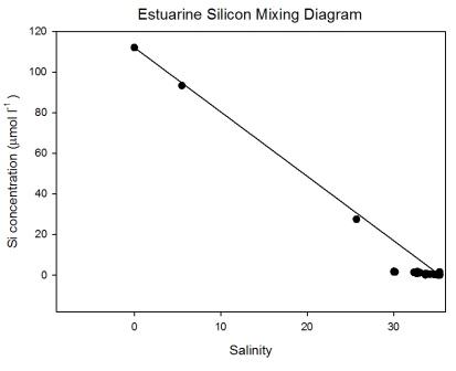
Figure 5.21 |
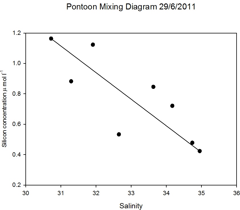
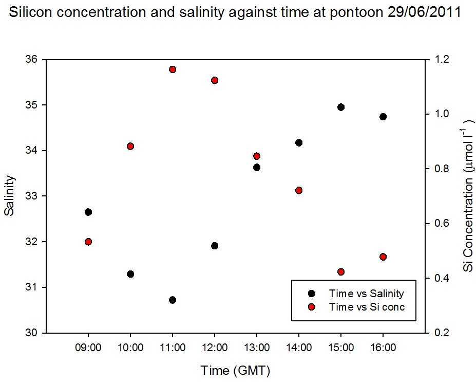
Pontoon
As observed in Figure
5.15 the salinity decreased an hour after low
water, when the silicon concentration was at a maximum of 1.2µ mol
l-1. When salinity was highest at 15:00GMT the silicon
had a minimum concentration of 0.4 µ mol l-1 (Figure
5.23). Figure
5.22 demonstrates that silicon was
behaving conservatively over the tidal cycle, illustrated by the
scattering around the theoretical dilution line. Therefore the
silicon concentrations observed at the pontoon were a product of
tidal mixing.
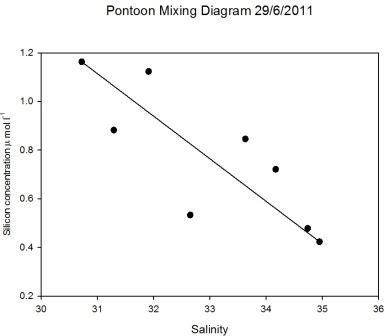
Figure 5.22 |
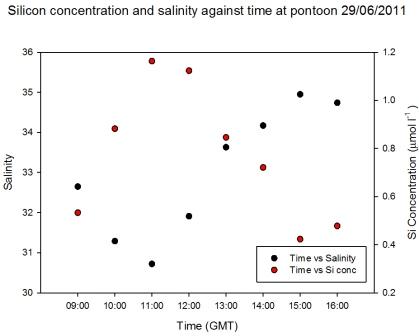
Figure 5.23 |
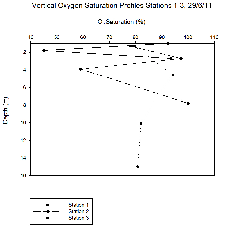
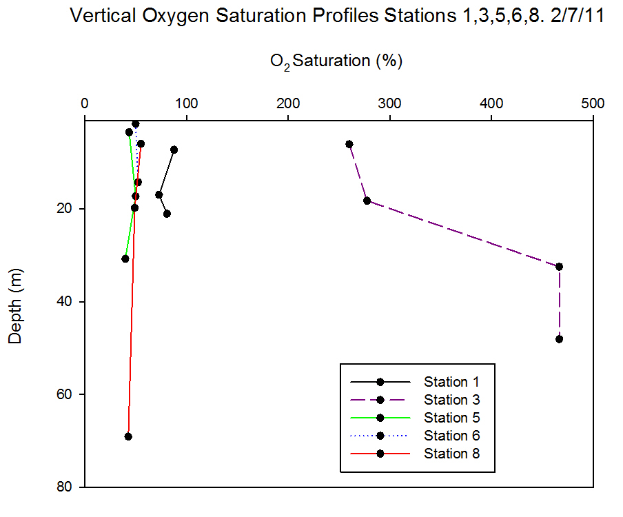
Dissolved Oxygen Analysis
Vertical
profiles of oxygen saturation from stations 1-3 are shown in
Figure 5.26.
Changes in oxygen saturation with depth may have been due to
zooplankton respiration. For example at station 1 there was a
decline in saturation at 1.8m, after which there was a gradual
increase with depth. At station 2 there was a decline in the surface saturation
from station 1 from 92.4% to 77.8%; this could have been due to an influx
of deoxygenated water or substance with a high biological demand.
Saturation increased with depth but then declined again at 4m. This
could be due to respiration or decomposition. Station 3, down river
of the mussel farm, had a surface saturation of 79.6%. Souchu
et al (2001) demonstrate how mussel farming can affect the
chemical properties of nearby water bodies.
The oxygen
saturation of the surface water is shown in
Figure 5.24; this graph
combines data from our 3 stations and group 11’s 5 stations. The
overall trend of surface oxygen saturation showed an increase from
the upper estuary at station 1 to the lower stations sampled by
group 11. There was a decline at stations 2 and 3, the highest
surface saturations were Group 11’s station 2 with 106.1% and station
5 with 104.2%.
The oxygen
saturation over the tidal cycle was shown in
Figure 5.25. The
data were collected at the King Harry Pontoon from 09:00 to
14:00GMT. There is a distinct change in oxygen saturation over the
tidal cycle. The highest saturation (102.4%) at 10:00 GMT corresponded with low
water at 09:52. There was a decline in saturation until 13:00GMT after
which the saturation increased again.
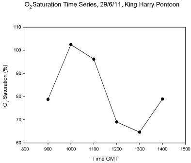
Figure 5.24 |
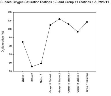
Figure 5.25 |

Figure 5.26 |
Phytoplankton & Zooplankton
Analysis
Estuary
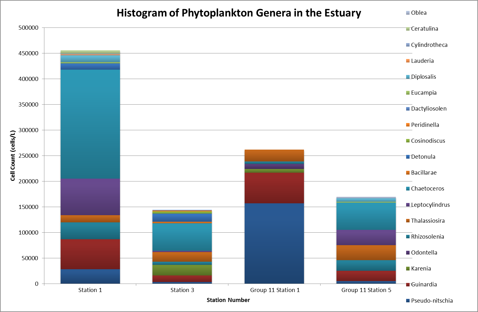
Phytoplankton
|
Phytoplankton abundance in
the Fal estuary was estimated by taking four samples
throughout the estuary. Group 6 collected samples at station
1 and station 3 at the top of the estuary. Group 11
collected their samples at group 11 station 1 and station 5
near Black Rock.
It was found that the
highest abundance of phytoplankton was at station 1 (Figure
5.27) which
corresponds with the zooplankton data, which show a high
number of copepods. At station 1 the most abundant
phytoplankton was the Chaetoceros genus as they were the
largest percentage (47%) of the sample at station one. Chaetoceros.
spp are planktonic diatoms, and would use the
dissolved silicon within the water to build their frustules;
this could cause dissolved silicon to be lower in areas of
high Chaetoceros abundance. This can be seen in Figure 5.21, which
shows that dissolved silicon is being removed within the
estuary at salinities above 30. This was the
area where large numbers
of diatoms were recorded. The smallest sample was at station 3;
this could be due to the nearby mussel farm. Studies have shown a relationship between mussel aquaculture
growth and a decline in nearby phytoplankton numbers (H.F.
Kasper, 1995). This is due to feeding processes of the
mussel;
the water and the organisms contained within it are passed
through siphon and particles are trapped within the gills.
Station 5 was the last
station for phytoplankton sampling, and is near the mouth of
the estuary. The percentage of the overall sample was
quite varied at station 5 where many genera were abundant,
for example Thalassiosira comprised 17% of the phytoplankton
population.
|
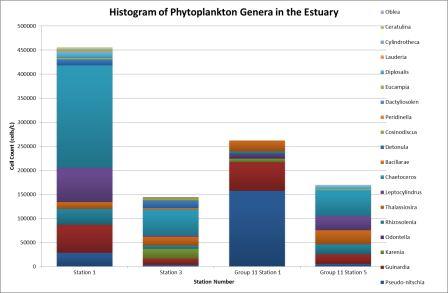
Figure 5.27 |
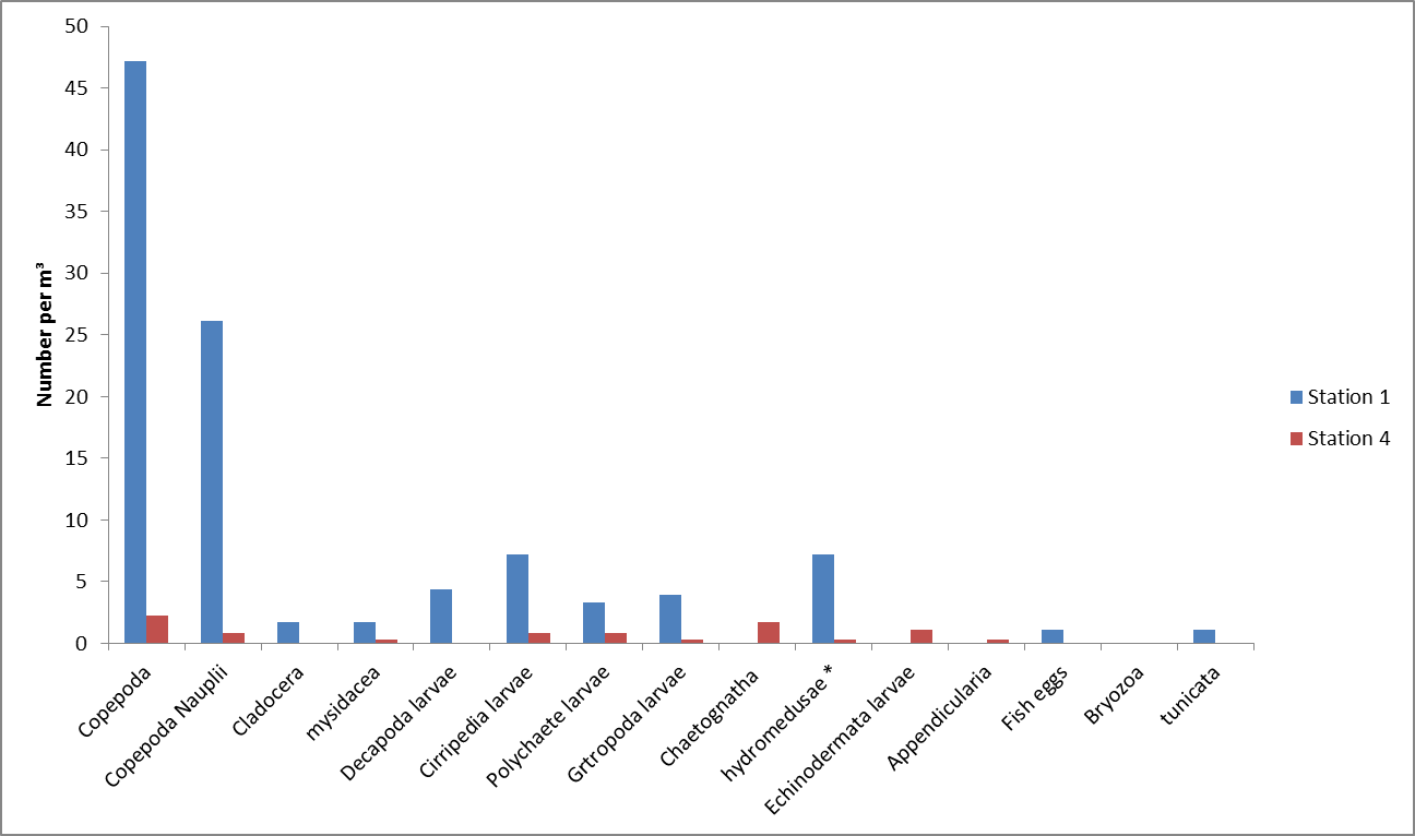
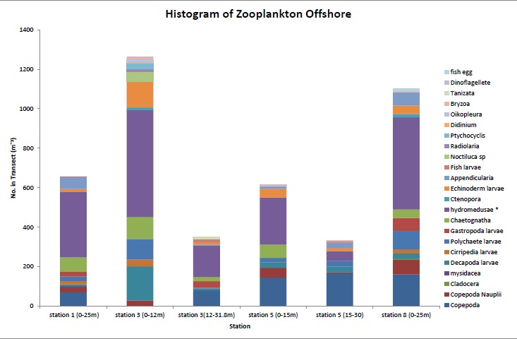
Zooplankton
|
Zooplankton abundance
was estimated by sampling at various stations throughout the
estuary. Group 6 collected samples at stations 1 and 4
located at the head of the estuary. From these
stations the highest abundance of zooplankton was at station 1 with
the most abundant type being holoplanktonic copepods which
made up 45% of the sample (Figure
5.28). This corresponds with the
phytoplankton data collected at the same station which show the highest abundance
sampled, the most
abundant of which was Chaetoceros curvisetus, a centric diatom. The lowest zooplankton abundance
was found at station 4 which was located near to the mouth
of the Truro River, close to where the Channals and Tolcarne
Creeks enter the river. Again the most dominant zooplankton
type were copepods however the low abundance could be the
result of the station being downriver from a mussel farm
meaning there were less nutrients available and fewer
phytoplankton.
|
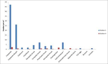
Figure 5.28 |
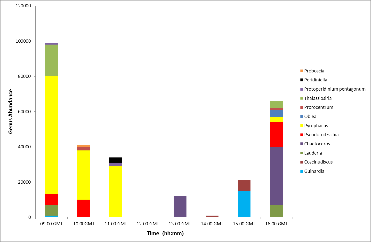
Pontoon
Phytoplankton
|
From 09:00 to 11:00GMT the
phytoplankton samples were dominated by Pyrophacus, a small
thecate dinoflagellate (Figure
5.29). After 12:00GMT the samples'
compositions appeared to vary with the dominant genera
becoming diatoms, the
prevalent genera being chaetoceros. This change in overall
composition from dinoflagellates to diatoms could be
attributed to the change in the tidal cycle. It could be
suggested that the rising tide pushed the dinoflagellates up
the estuary. However, it could also be suggested that the dinoflagellates moved deeper in the water column so would
not have been sampled as all water samples were taken from
the surface. It is also important to note that the
Pyrophacus may have been misidentified in the laboratory as small thecate
dinoflagellates are often difficult to differentiate from each
other.
|
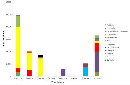
Figure 5.29 |
Chlorophyll Analysis
The chemical chlorophyll analysis conducted from water samples in
the lab shows a trend from low chlorophyll concentrations (< 2 µg
l-1
) in the uppermost estuary increasing to a maximum at station 2 (> 6
µg l-1) (Figure
5.30). The concentrations begin to decrease to ~ 4 µg l-1 at station 3
and ~ 3 µg l-1 at station 4. In the lower estuary concentrations are
lower at Group 11 station 1 < 1 µg l-1, increasing to ~ 2 µg
l-1 at
Group 11 station 2 and ~ 3µg l-1 at Group 11 stations 3-5. The
sampling was taken from low tide at the top of the estuary to high
tide at group 11 sampling stations.
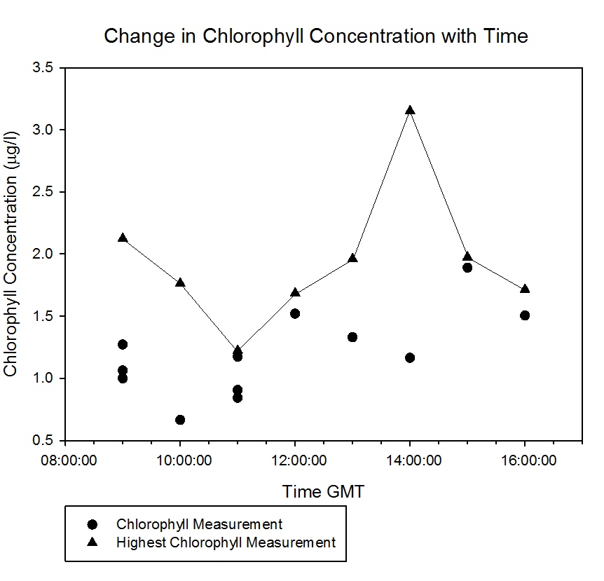
The chlorophyll temporal analysis at the pontoon (Figure
5.31) shows a
relationship between the chlorophyll concentrations and the tidal
cycle as the chlorophyll decreases at the tide ebbs and increases as
the tide floods. There is a slight tidal lag but a clear
relationship
as more phytoplankton were being washed up the estuary with the
tide.
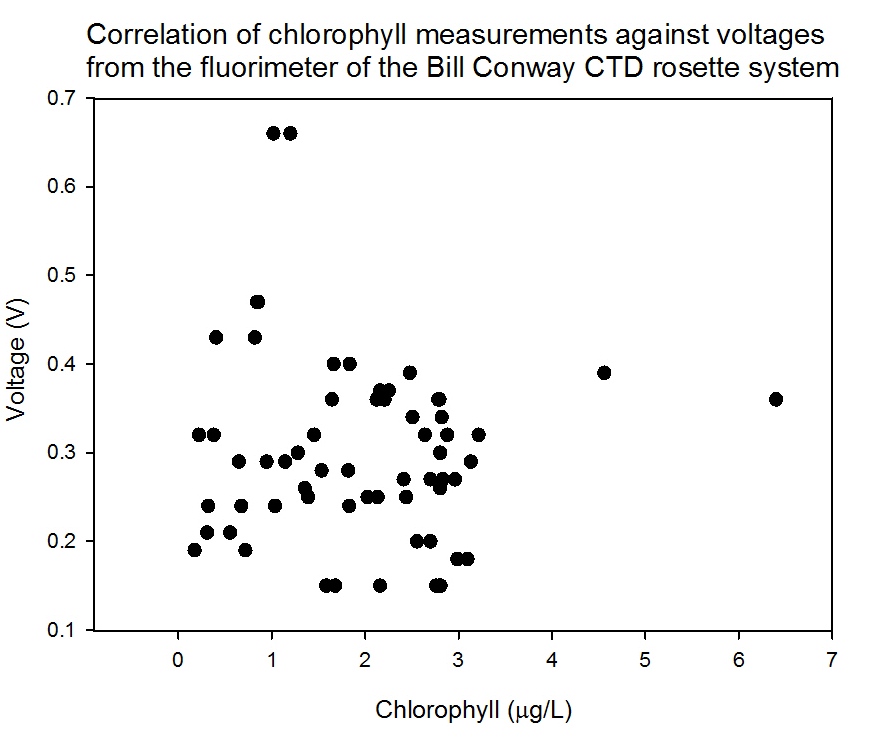
Calibration of the chlorophyll data plotted from laboratory analysis
against the voltage gained by the fluorometer on the
CTD shows an
unclear and weak relationship (Figure
5.32), but not enough to
develop a clear relationship between the voltages and the chemical
chlorophyll analysis. The chlorophyll laboratory equipment has
provided some inconsistent results, but the trends observed and
described above should still show relative patterns, though the
exact Figures might not be reliable.
The chlorophyll analysis does not correspond very well to the
phytoplankton count analysis; for example the phytoplankton count
demonstrated a higher number of phytoplankton at station 1 compared
with station 3 when the chlorophyll analysis suggests that in fact
at station 3 the chlorophyll concentrations and therefore the
phytoplankton populations may have been twice as great. This might
be partially explained by the differences in chlorophyll
concentration in different phytoplankton cells, and therefore the
most numerous species not necessarily being the most chlorophyll
rich. In addition there are inconsistencies with chlorophyll data
and replicates which is becoming apparent as a general trend across
all groups and may be due to methodology or equipment error. The
oxygen data however corresponds well as there are lower dissolved
oxygen concentrations at Group 6 stations 1 and 2 – the highest
concentration chlorophyll stations. This is an expected finding as
chlorophyll concentrations indicate a higher population of
phytoplankton which deplete the oxygen concentrations due to
photosynthesis. Nutrient analysis shows addition of phosphate, but
no depletion of either phosphate or silicon. Therefore the
chlorophyll concentrations in the estuary do not indicate a
phytoplankton population of enough significance to cause nutrient
removal, though any removal may be countered by agricultural/sewage
inputs in the case of phosphate (discussed
above).
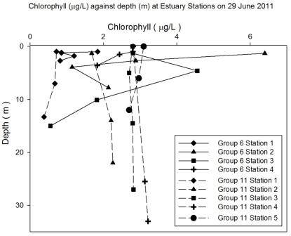
Figure 5.30 |
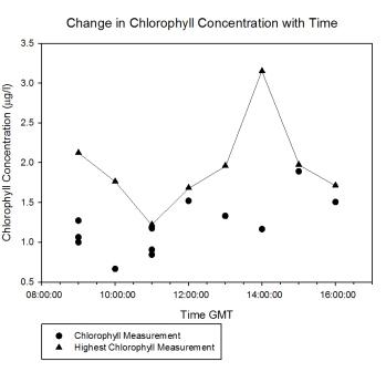
Figure 5.31 |
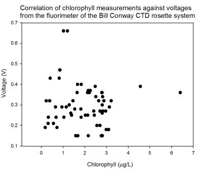
Figure 5.32 |
Conclusion
The data obtained in the estuary demonstrate the characteristics of
the Fal Estuary at the time of sampling and reflects expected
characteristics for a temperate estuary such as the Fal. The
sampling up the estuary reflected a greater freshwater influence at
the top compared to towards the mouth, but the salinity variation
was not large due to freshwater inputs not being sizable in the
region. Warmer temperatures were sampled at the top of the estuary
than at the bottom, but the tide was low when sampling the shallow
top of the estuary so the water column would have been much easier
to warm than near the deeper mouth at high tide. Greater
phytoplankton populations are demonstrated at the top of the
estuary, which appear to support greater zooplankton populations
near the top. The high nutrients are not utilised to a degree that
indicates significant removal and indeed phosphate addition was
observed due to high agricultural, sewerage and mine drainage inputs
into the Fal. The high productivity near the top of the estuary has
depleted the dissolved oxygen relative to the bottom of the estuary
where values measured are much higher. Particularly at station 3
dissolved oxygen was depleted but the phytoplankton also remained
low; station 3 was taken by a mussel farm which may cause the oxygen
depletion and also restrict the phytoplankton population.
|
Offshore        |
Introduction
|
The offshore boat
practical aimed to investigate the vertical mixing processes
in the waters of the Western English Channel off Falmouth.
They usually become vertically stratified during the summer
months due to lower wind mixing and higher irradiance
levels, but the shallow waters next to the coast remain
mixed. Fronts therefore form in the channel, with warmer
water above cold water on the stratified side and mixed
cooler water on the coastal side. Fronts often tend to have
large plankton communities due to the nutrients provided by
the mixed side but the stratified waters allowing the
plankton to remain in the high irradiance surface waters.
The systems offshore along the coast around Falmouth were
therefore investigated to observe how the vertical processes
affect the plankton communities. The physical measurements
made by instruments aboard a CTD would be compared with
chemical data from water sampling and the biological data
from phytoplankton samples and zooplankton trawls to observe
how the physical processes control the biological
productivity.
The primary plan for the offshore day
was formulated based on data from the previous day's group
(Group 3) who had travelled west from Falmouth along the
coast towards Lizard Point and discovered frontal systems
along the 30m contour. Based on this, Group 6 planned to zig-zag across the frontal system out to 50m and back in to
20-30m along the coast from the Manacles to Lizard Point.
Samples were collected from stations along the frontal
systems appropriate to the findings in the field indicated
by the thermo-salinometer and the acoustic doppler current
profile. An overview of each station is provided below in
Table 6.1.
Although a number of stations were fully sampled, due to
time constraints only a CTD drop occurred at others in order
to gain a larger set of physical data relating to the front.
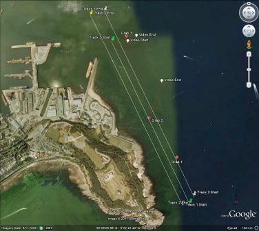
In case of the primary plan not yielding
a change in physical processes (being constantly monitored
onboard by the ADCP and thermo-salinometer) the secondary
plan would be to head out directly offshore until a change
from mixed waters to stratified waters was observed and then
to sample either side of and on the frontal system. In the
event, the secondary plan was not required and the path
taken is displayed in
Figure 6.1.
|
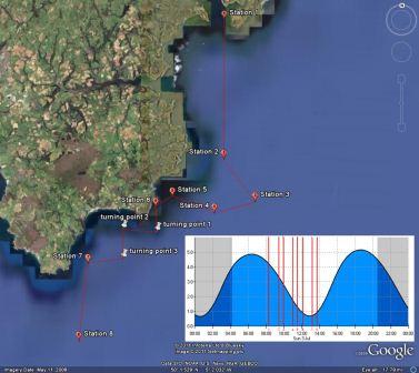
Figure 6.1 |
|
Station Number |
Latitude (WGS84) |
Longitude (WGS84) |
Activity |
| 1 -
Black Rock |
50°08.662 N |
005°01.486 W |
A full sample station was taken at Black
Rock. This station has been sampled by every group
on Callista and therefore
together the data will provide a temporal series of data at
the site over 10 days. |
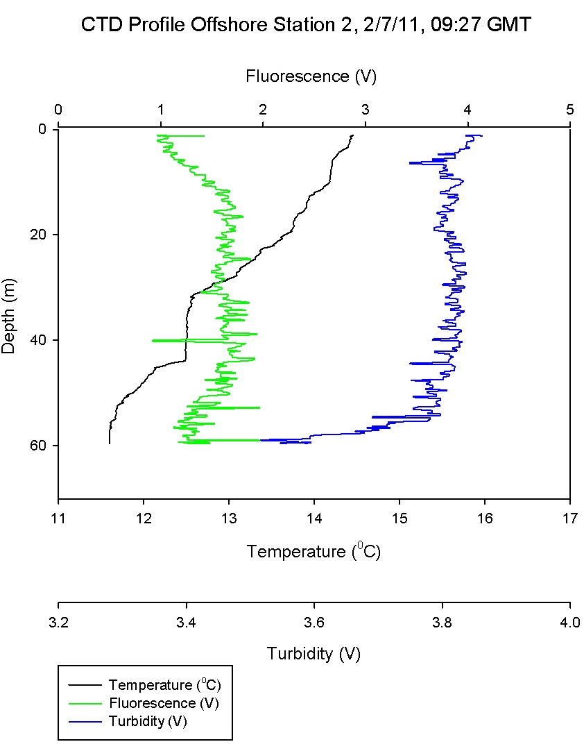
| 2 -
The Manacles |
50°02.693 N |
005°01.151 W |
CTD drop only. A continuously stratified station.
|
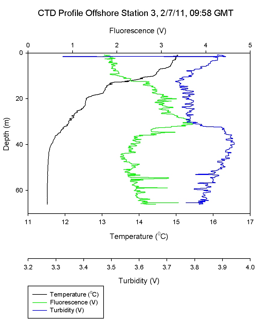
| 3 -
Offshore of the Manacles |
50°00.927 N |
004°58.975 W |
Full sample station. Stratified |
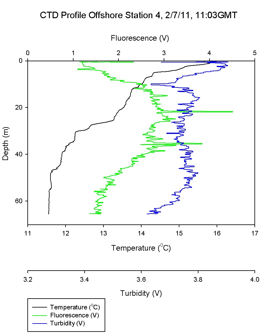
| 4 |
50°00.385 N |
005°01.641 W |
CTD drop
only. Stratified station. A high backscatter anomaly seen on
the ADCP prompted the group to deploy the CTD at this
station to investigate. |
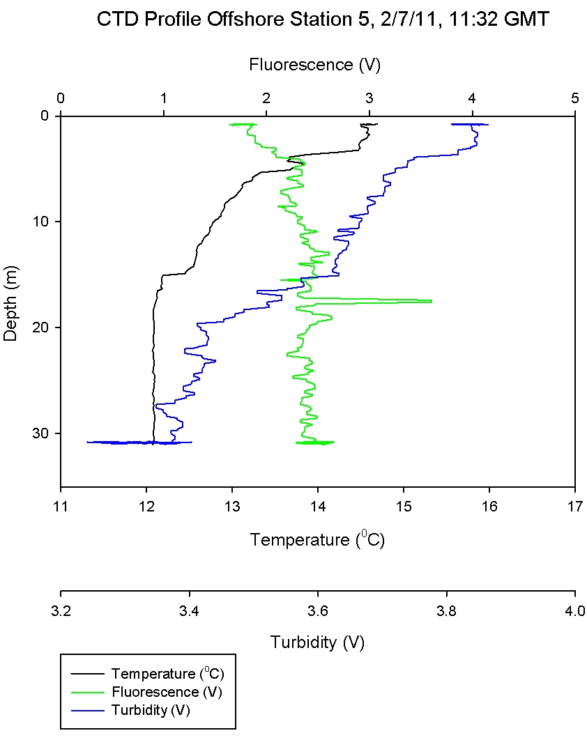
| 5 |
50°00.991 N |
005°04.455 W |
Full station. Stratified station with high chlorophyll
levels throughout suggested that the station had recently been
mixed. |
| 6 |
50°00.524 N |
005°05.536 W |
Full station. Water column mixed indicating the
station was inshore of the frontal systems.
|
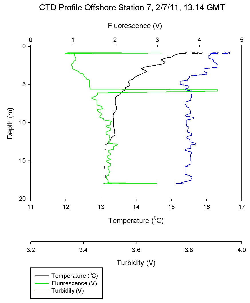
| 7 |
49°58.017 N |
005°09.850 W |
CTD drop only.
Partially mixed station investigated whilst heading towards
Lizard Point due to multiple crossings of a frontal system
indicated by a marginal temperature rise and ACDP data, as
well as visually indicated by a change in water
colour causing stripes to form across the ocean. |
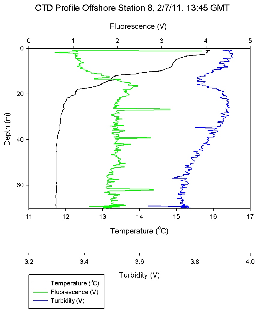
| 8 -
Offshore Lizard Point |
49°54.715 N |
005°10.230 W |
Full station. Stratified station directly offshore
Lizard Point. |
Table 6.1
Physical Characteristics
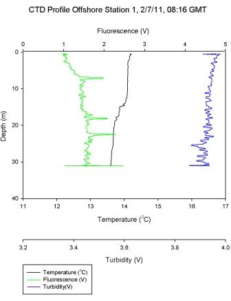
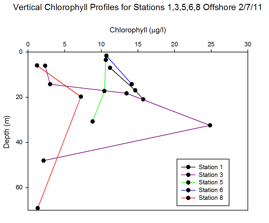
Figure 6.2 - Station 1 |
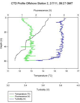
Figure 6.3 - Station 2 |
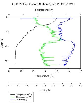
Figure 6.4 - Station 3 |
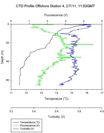
Figure 6.5 - Station 4 |
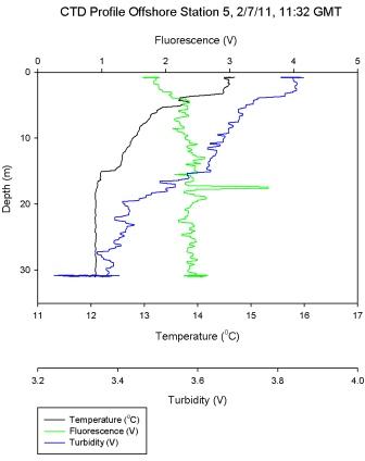
Figure 6.6 - Station 5 |
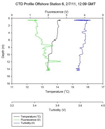
Figure 6.7 - Station 6 |
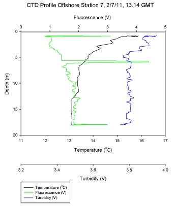
Figure 6.8 - Station 7 |
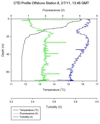
Figure 6.9 - Station 8 |
Richardson's Number
The Richardson's (“Ri”) number can be calculated and used to
describe the nature of the water column; Ri<1 describes
turbulent flow, Ri<1/4 describes laminar flow and an Ri
number in-between these values expresses gravitational
shear. It can be calculated using the following equation:
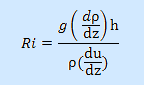
|
Ri is dimensionless |
h= depth (m) over
which density/ velocity are compared
|
|
g=9.81 m s-1 (gravitational force)
|
ρ= average density (kg m-3) in the water column |
|
dρ/dz= change in density (kg m-3) with depth |
du/dz= change in velocity (m s-1) with depth |
Ri depth profiles were plotted for each fully sampled
station and were used with CTD profiles to
help describe the balance of the stabilizing forces, such as
buoyancy, on flow over the destabilizing forces, such as
vertical shear.
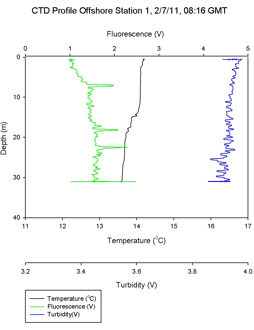
Figure 6.2 shows that the water column at
Black Rock was quite stratified with a warmer layer on top
of a cooler layer with salinity and chlorophyll remaining
relatively constant through both of the layers. The gradual thermocline
seen between 15-20m in
Figure 6.2
has high levels of laminar flow as shown by an increase in
Richardson number in Figure 6.10. The stratified water above has low Ri
values and thus is shown to be turbulent; with mixing
present.
Figure 6.4
shows a stepwise thermocline in
stratified water, with sharp decreases in temperature at
10m, 18m, and 22m. The main thermocline boundary is at 40m
after which there is a mixed water layer. Cross analysis
with the Ri number in Figure 6.11 shows laminar flow at each of these depths and turbulent
water bodies in between. Turbulent water persists once the
mixed layer boundary has been crossed, as is shown by a Ri <
0.25. Some fluctuations in the Ri number may be explained by
this ‘snap shot’ view of the water column which captures
where small variations in shear or buoyancy dominate, but
does not describe the general water body trend.
Figure 6.6
shows a frontal water column that
has recently become stratified. This is evident due to
uniform levels of chlorophyll throughout the water column. A
steep thermocline at 5m corresponds to high Ri numbers on
Figure 6.12. The thermocline
weakens and becomes more gradual to 15m, where a low Ri
number depicts more turbulent flow and mixing. The likely
recent mixing of this water column may explain other
fluctuations in the data, as does the snap shot nature of
this survey as described above.
Figure 6.7 shows a steep temperature gradient at 9m,
corresponding with a high Ri number as would be expected in
a thermocline. As the temperature gradient is crossed and
the water cools turbulent flow becomes predominant once
more. At most other depths in the water column low Ri values
describe turbulence and a well-mixed system.
Figure 6.9 was an additional offshore stratified station to
complement station 3. However, station 8 lacks the steep thermocline seen in station 3, instead a gradual thermocline
occurs from the surface to 20m. Within this surface
stratification, high Ri numbers as shown in
Figure 6.14, and may fluctuate due to
internal currents. Once the mixed layer boundary has been
crossed low Ri numbers describe turbulence and deep water
mixing.
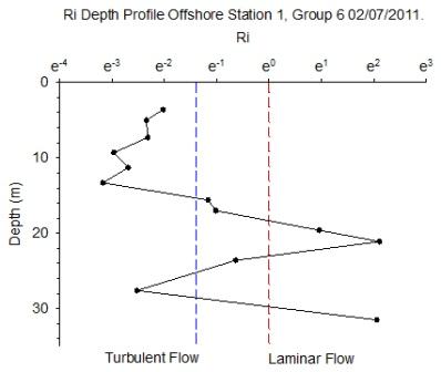
Figure 6.10 - Station 1 |
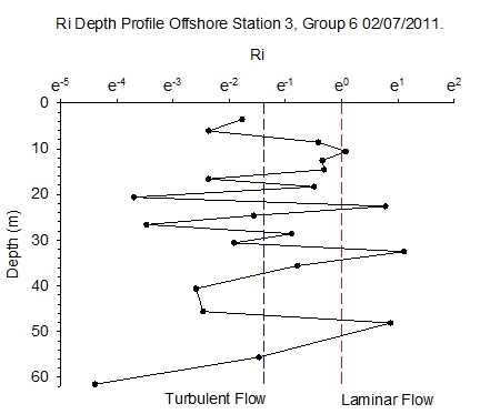
Figure 6.11 - Station 3 |
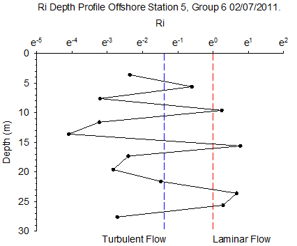
Figure 6.12 - Station 5 |
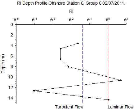
Figure 6.13 - Station 6 |
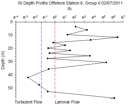
Figure 6.14 - Station 8 |
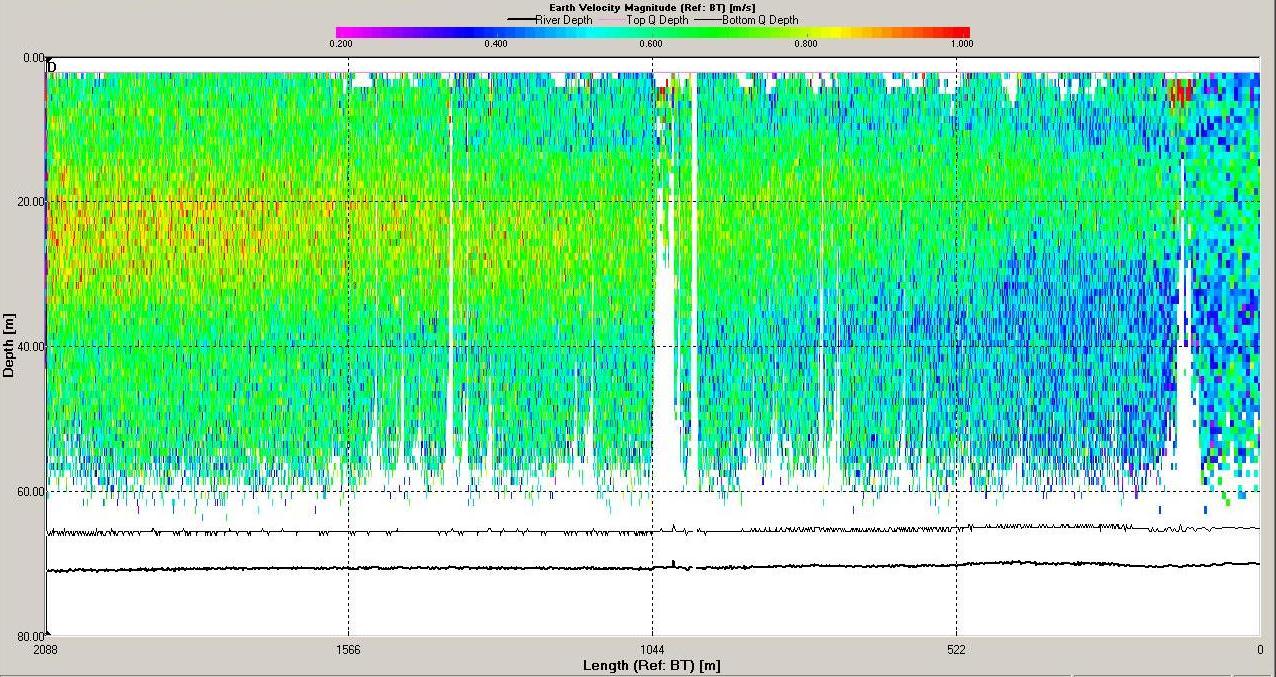
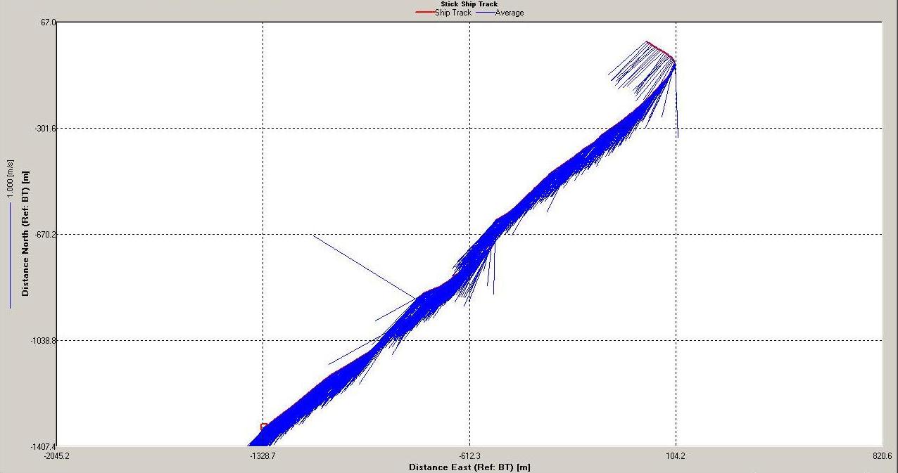
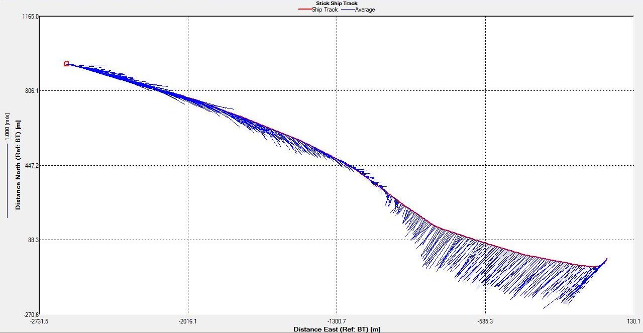
ADCP
Analysis
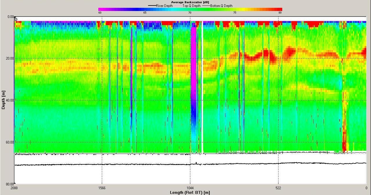
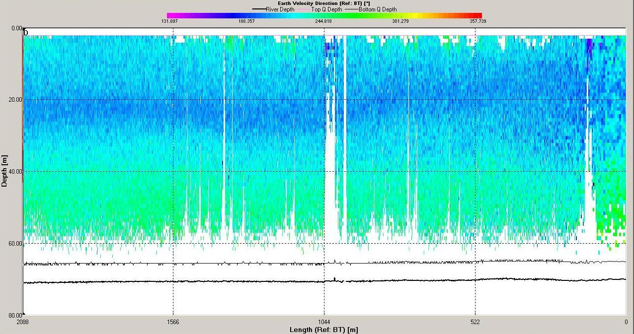
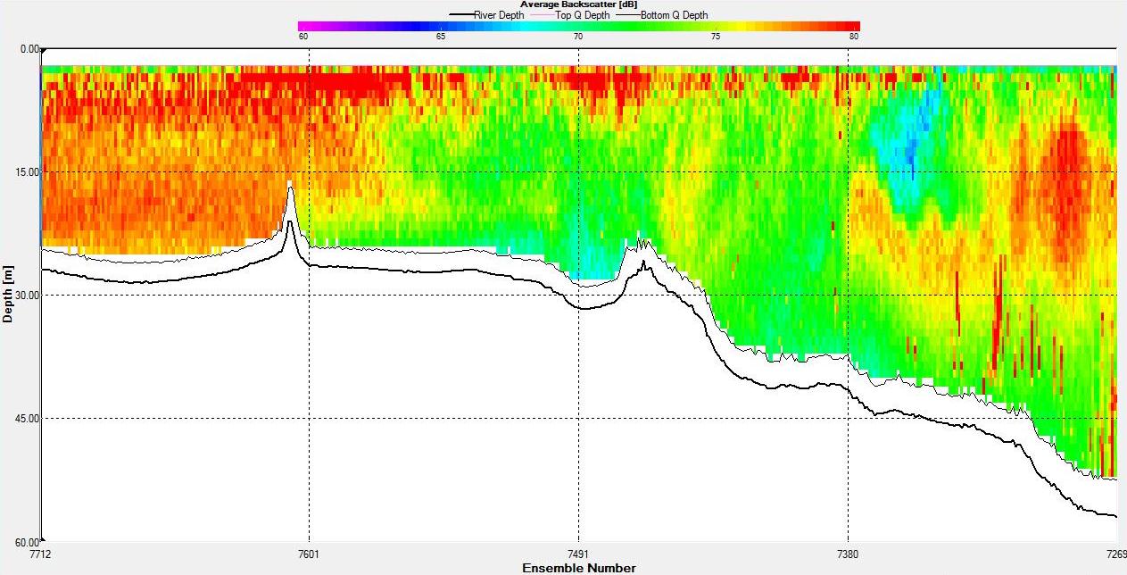
Figures 6.15,
6.16,
6.17 and
6.18 show the ADCP
data for station 3 where the water was stratified. The
backscatter shows a band of high backscatter around 20-30m
reflecting zooplankton populations
feeding on phytoplankton which reside around the thermocline
where they can access nutrients in the lower layer. The
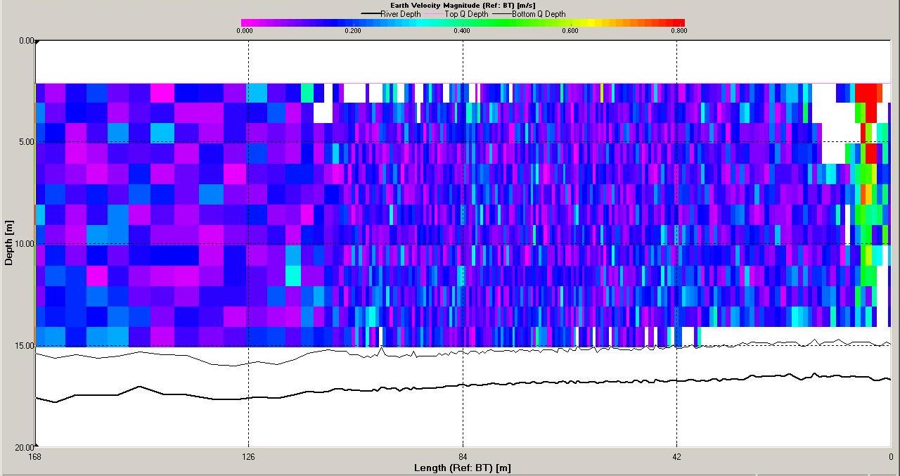
magnitude of velocity was low at this station with minimum
values around 0.4m s-1 and maximum around 0.9m s-1.
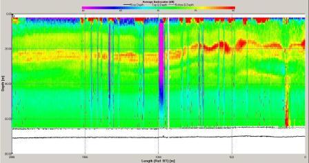
Figure 6.15 Backscatter
|
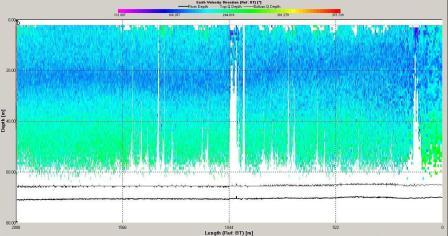
Figure 6.16 Velocity Direction |
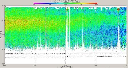
Figure 6.17 Velocity Magnitude |
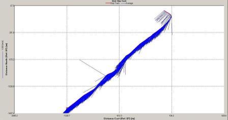
Figure 6.18 Stick |
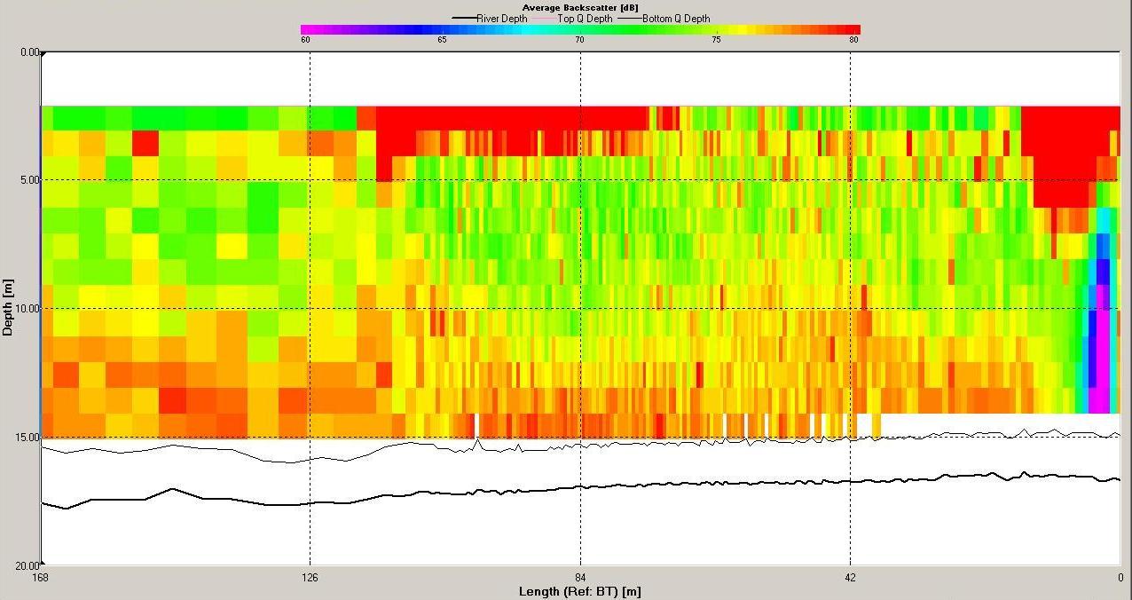
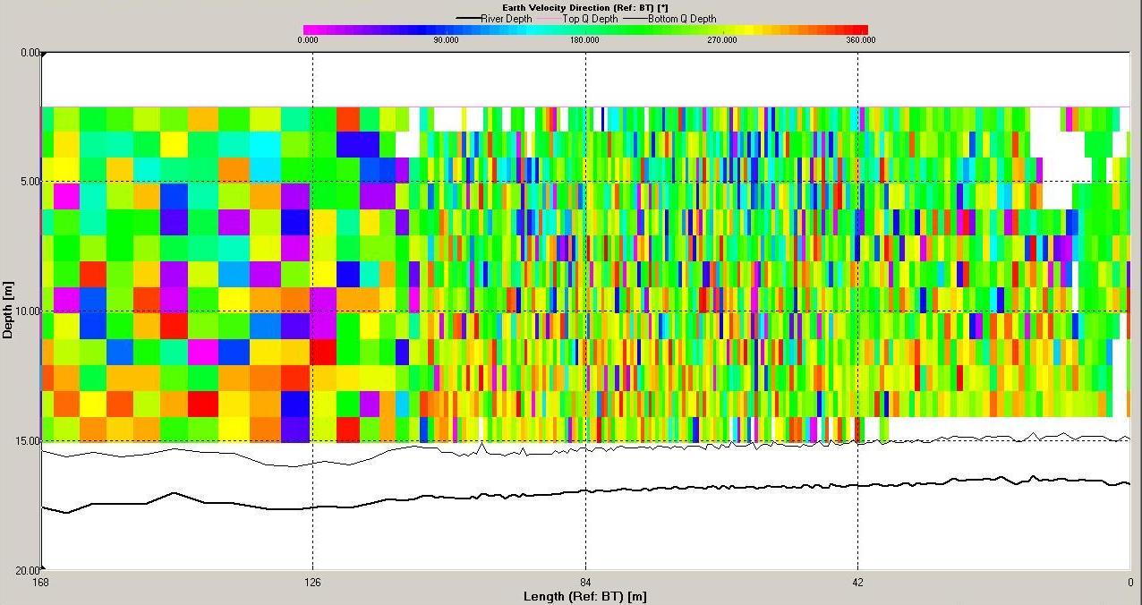
The ADCP data for station 6 (illustrated in Figures
6.19,
6.20
and 6.21) demonstrate that the water column was mixed.
Backscatter here was high across the water column compared
with stratified stations as at mixed stations the
higher
nutrient concentrations (see
phosphate and silicate) throughout the water column allow
phytoplankton and therefore zooplankton populations to
remain high. Shear flow can be observed in the velocity
direction plot with direction varying from 0 to 360o. The
velocity observed at station 6 is lower then at station
3 with maximum value around 0.5ms-1 and a minimum of 0.05ms-1.
The velocity of tidal flow may vary depending on the
location and position along the coast with features such as
headlands affecting the velocity measured.

Figure 6.19 Backscatter |
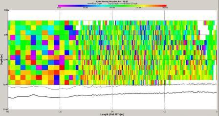
Figure 6.20 Velocity
Direction |
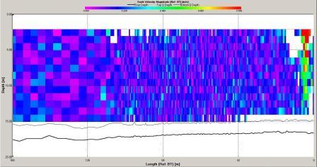
Figure 6.21 Velocity
Magnitude |
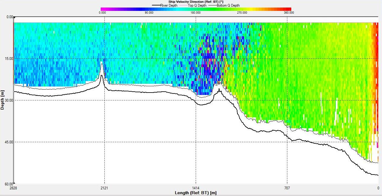
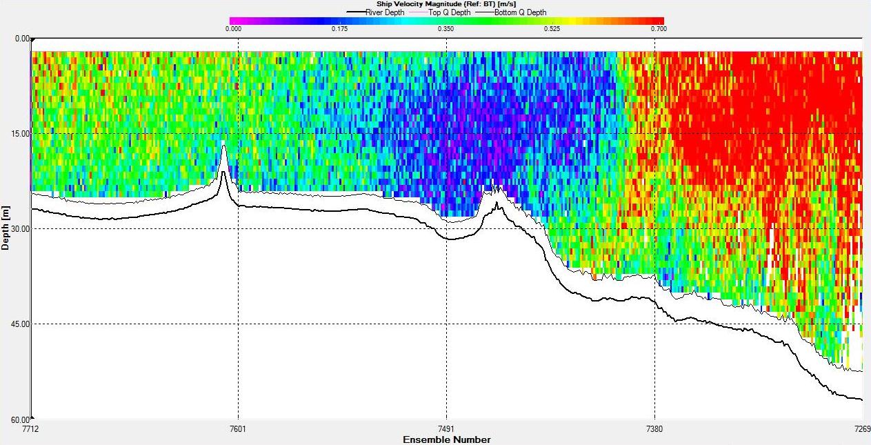
Figures 6.22,
6.23,
6.24 and
6.25 show a tidal front
that was observed on the ADCP. The
backscatter plot shows lower backscatter than at either side
of the front. Velocity direction goes from around 200°
on the eastern side of the front to around 100° on the western side
with shear flow in the middle at the front. In addition, the
velocity at the front is low compared to either side with
the eastern side having a flow of around 0.7ms-1 and the front
having a flow of 0.1ms-1.
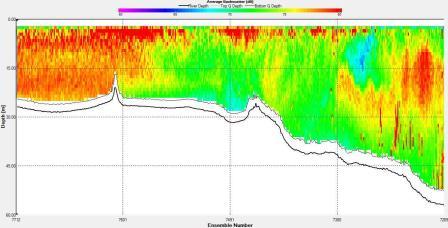
Figure 6.22 Backscatter |
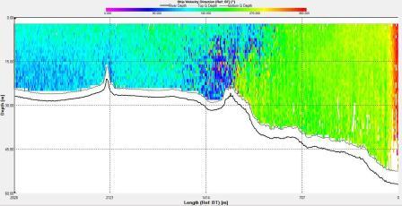
Figure 6.23 Velocity
Direction |
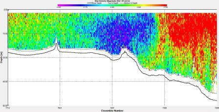
Figure 6.24 Velocity
Magnitude |
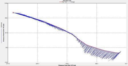
Figure 6.25 Stick |
The
position of the tidal front was obtained by using ADCP data obtained whilst zig-zagging between Black Head and
Lizard Point. The latitude and longitude (using WGS 84) of three points
along the front are plotted on the following Google Earth
plot (Figure 6.26). The points plotted on the admiralty chart
in Figure 6.27 show that the front is positioned between the 27
- 33m contour.
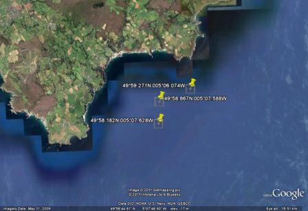 Figure 6.26
|
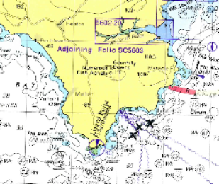 Figure 6.27
|
Stratification Parameter
|
The stratification parameter
log(h/u^3) (where h is the depth and u the tidal
current) gives
an indication of the degree of mixing in the water
column due to tides and wind or the degree of
stratification enhanced by heat input, freshwater
inputs, and increased water depth. As a general
rule, the stratification parameter tends to be < 2 at
mixed stations and >3 at stratified stations. At a
tidal front the value may be approximately log (h/u3) =
2.7± 0.3 for a tidal front (as suggested by Simpson
and James (1986)). At station 1, the station was
well stratified: the stratification parameter value 3.65
(Table 6.2) is corroborated by the CTD
data. Stations 3,5 and 6 are all relatively close to
the tidal front and so show stratification parameter
between 2 and 3. For example, station 5 was observed
in the CTD data to have a stratified water column
with respect to temperature, but high chlorophyll
levels throughout the water column suggested that
the water column had been recently mixed. This
demonstrates how the tidal front moves as the
balance of mixing due to tide and winds and heat
input varies. Station 8, offshore of Lizard Point,
was well stratified and the stratification parameter
corroborates the data gained from the CTD at this
station. As R. V. Callista neared station 8, a temperature
of >17°C was recorded on the thermo-salinometer
which was the highest surface water temperature that
had been recorded offshore for the preceding week. This
illustrates the increasing solar irradiance/heat
input and how its balance with the tidal and wind
mixing would affect the position of the tidal front
during the fieldcourse (especially as the weather
was generally fine with low winds). |
|
Station |
Depth, h (m) |
Tidal Strength, u
(ms-1) |
(h/u3) |
Stratification parameter
log(h/u3) |
|
1 |
31.5 |
0.191 |
4495 |
3.653 |
| 3 |
61.5 |
0.628 |
248 |
2.394 |
| 5 |
30.8 |
0.536 |
200 |
2.301 |
| 6 |
14.3 |
0.367 |
289 |
2.460 |
| 8 |
62.0 |
0.295 |
2418 |
3.383 |
Table
6.2 |
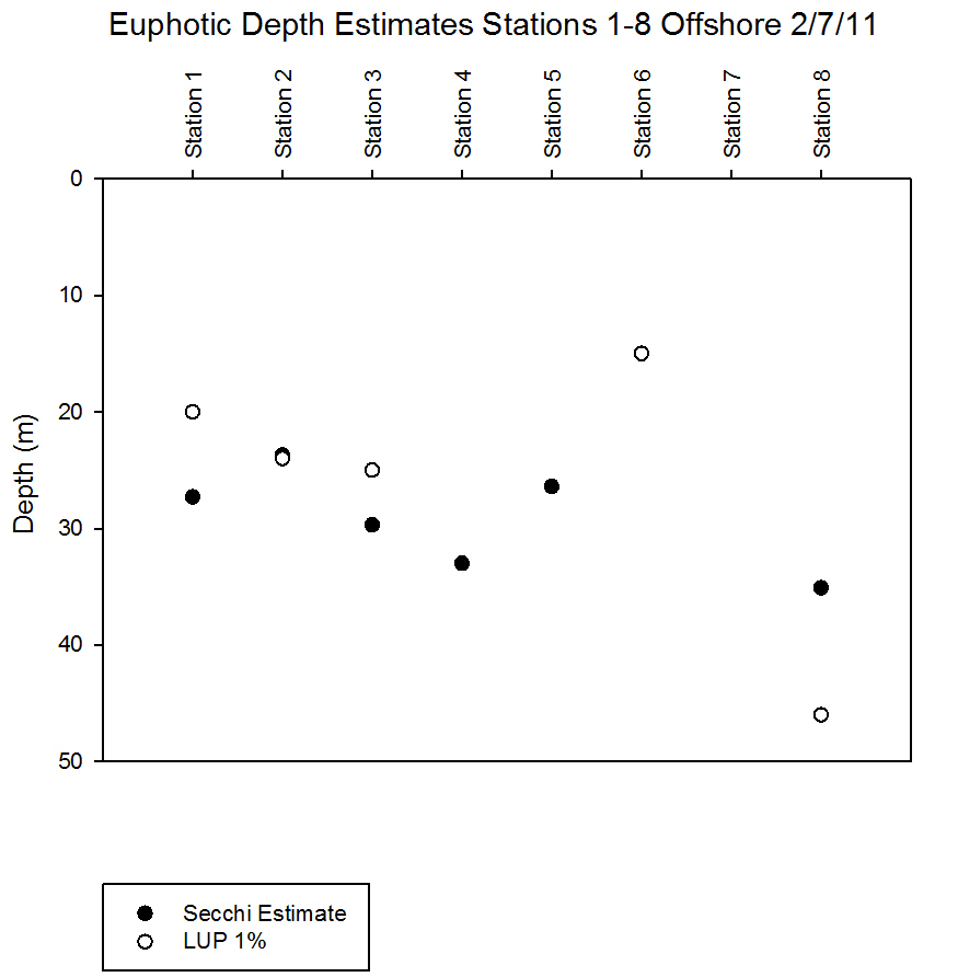
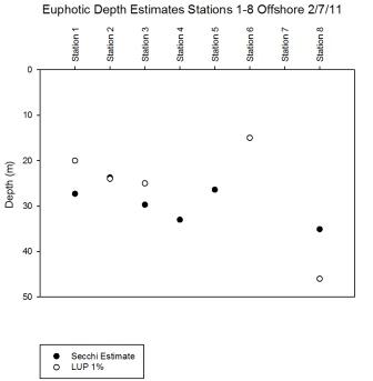
Light Analysis
|
Secchi disk measurements were used to estimate
the depth of the euphotic zone for the offshore
stations. This is defined as the area with
sufficient light for photosynthesis. The LUP
measurements from the
CTD can also be used as a euphotic depth
estimate by finding the 1% light level. Both
estimates suggested that the deepest euphotic zone was
found at station 8 (Table 6.3), this station also had the lowest
k value and therefore slowest attenuation of light.
Station 8 was strongly stratified suggesting lower
mixing in the surface layer so reduced turbidity. As
shown in
Figure 6.28 there is a difference of 11m between
the Secchi and LUP estimates, the LUP 1% is
considered to be more accurate, and the fluorescence
CTD readings indicated the presence of chlorophyll at
the LUP depth as shown in
Figure
6.9.
These estimates should be used
as a rough guide to the euphotic depth and this
cannot be understood fully until chlorophyll and
fluorescence are analysed. In all cases the LUP
depth should be considered as the most reliable when
identifying relationships.
Note that the Secchi disk euphotic
depth estimates for station 6 and 7 are deeper than
the water column. Therefore the entire water column
was contained within the euphotic zone and could
expect to receive sufficient light for photosynthesis from
the
surface to the bed. However the LUP 1% was much
shallower at station 6 suggesting an inaccurate
Secchi estimate. The 1% light level was not reached
for stations with marked * in Table 6.3.
|
Station |
Secchi Depth |
Euphotic Depth
Estimation (m) |
k - Attenuation Coefficient |
LUP 1% Light
Depth (m)
|
| 1 |
9.1 |
27.3 |
0.15 |
20 |
| 2 |
7.9 |
23.7 |
0.18 |
24 |
| 3 |
9.9 |
29.7 |
0.15 |
25 |
| 4 |
11.0 |
33.0 |
0.13 |
* |
| 5 |
8.8 |
26.4 |
0.16 |
* |
| 6 |
8.6 |
25.8 |
0.17 |
15 |
| 7 |
9.5 |
28.5 |
0.15 |
* |
| 8 |
11.7 |
35.1 |
0.12 |
46 |
Table
6.3 |
Figure
6.28 |
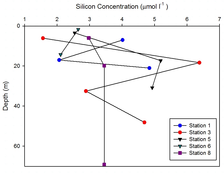
Dissolved Silicon Analysis
|
Station 1
(Figure 6.29) showed a decrease in measured dissolved silicon
concentration at 17m which increased down to 20m to 4.8
µmol l-1. On the CTD data a strong thermocline
was illustrated down to 21m, this prevented
the dissolved silicon mixing below the thermocline.
This correlates with
Figure 6.32 which
shows an increase in phytoplankton abundance at this
depth and suggests that they are utilising the silicon
source, resulting in a decreased silicon concentration
at this depth.
At station 3 measured dissolved silicon
concentration increased to 6.4 µmol l-1 at 18m,
then decreased with depth. The CTD data showed a
very shallow surface warmed layer and a deep thermocline, below which chlorophyll
increased (Figure
6.4). An increase in chlorophyll is a proxy for
phytoplankton abundance and suggests the decrease in
silicon concentration at 32m may have been due to the utilisation
of dissolved silicon.
At station 5 silicon concentration increased to 5.2
µmol l-1 at 17.3m. The shallowest warmed layer
at station 5 (Figure
6.6) may have forced the immotile phytoplankton to the
very surface which is where lower silicon concentrations
were observed
indicating utilisation. The dissolved silicon
concentration showed an increase at depth at 17m
indicating replenishment just below the thermocline.
From surface to 14.3m, measured silicon
concentrations at station 6 decreased by 0.5 µmol l-1.
Figure
6.7 showed that the water column at
this station had weak stratification. This was
reflected by the low concentrations measured as
there is no strong stratification keeping the
silicon in the shallower depths sampled.
At station 8 silicon concentration showed no measured
changes with depth after 3.5m, with slight depletion
in the surface waters.
Figure
6.9 showed a strong thermocline down to 20m below which temperature and salinity data
indicated well mixed waters. Also below 20m
fluorescence remained homogenous with depth,
suggesting phytoplankton were also mixed within the
water column, which may have explained the lack of measured
changes in dissolved silicon concentrations. |
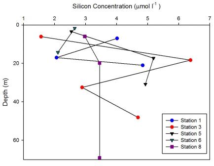
Figure 6.29 |
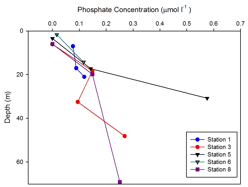
Phosphate Analysis
|
At Station 1
no measured changes in phosphate
concentration were observed with
depth (Figure
6.30). This is reflected in the
CTD data (Figure
6.2) which shows no significant
changes in fluorescence with depth, indicating very
low biological activity at this point.
At station 3 measured phosphate concentration showed a general
increase with depth. However at 32.5m phosphate
decreased to 0.09 µmol l-1. At this depth (Figure
6.4) shows an increase in fluorescence implying
increase of phytoplankton abundance. Phosphate being
a macronutrient may be being
utilised at this depth and has the potential to
become limiting over time.
Station 5 shows a measured increase of phosphate
concentration of 0.6 µmol l-1 at depth 30.8m. (Figure
6.6) shows that this depth is in the
mixed layer below the thermocline suggesting that
the increase in phosphate was due to remineralisation.
However also at this depth the phytoplankton data
show abundance in Thalassiosira. This genus of
phytoplankton are surviving at this depth as they
are in the photic zone, however it is likely they
have not got sufficient light to utilise the
phosphate to the point of depletion.
Phosphate concentration at station 6 increased from
0.02 µmol l-1 at depth 1.7m to 0.12 at depth 14.3m.
(Figure
6.7) shows that the thermocline exists down to about 15m, above
which phosphate was more depleted than below where it
is being replenished.
Measured phosphate concentration at station 8 showed a very
similar profile to measured silicon concentrations (Figure
6.29); showing no measured change in
concentration with depth from 19.8m. There was depletion in
the surface waters, with 0 µmol l-1 at
6.1m. (Figure
6.9) shows a strong thermocline down
to 20m below which temperature and salinity
data indicate well mixed waters. Also below 20m
fluorescence remains homogenous with depth,
suggesting phytoplankton are also mixed within the
water column therefore unable to utilise phosphate
which can explain the lack of observed changes in
phosphate concentration. |
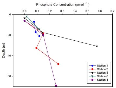
Figure 6.30 |
Dissolved Oxygen
|
Station 1 (Black Rock) was well-mixed with
low background concentrations of chlorophyll and no
significant chlorophyll peaks; this is reflected in
the homogeneity of the oxygen measurements taken
over the range of depths (7.3m to 21.1m) (Figure
6.31). Due to
the attenuation of light through the water column,
chlorophyll concentration decreases with depth as does rate of photosynthesis
and therefore the drop in
oxygen concentration may be explained.
Station 3 was offshore at a stratified water column with the strongest recorded thermocline of the offshore stations. The water was
supersaturated with oxygen (260.1% at surface,
466.6% at 32.5m) and the peak in oxygen saturation
coincided with the peak of chlorophyll at 32.5m
(24.8µg l-1).
Station 5 was inshore on a body of water that had
recently been mixed and was weakly stratified at the
time of sampling. Variation between the oxygen
measurements taken across the warmed surface layer was small. A small rise in
oxygen concentration was measured at 17.3m which
coincided with a small peak of chlorophyll at the
same depth.
Station 6 was inshore on a well-mixed body of
water. The oxygen measurements showed little
variation and CTD data show the homogeneity of the
water column.
Station 8 was on a stratified water body
and yet the oxygen data show there was little variation
over a large depth range (6m to 69m). Despite the
presence of a chlorophyll maximum, turbidity minimum and
strong thermocline at 12.5m, the oxygen saturation
remained stable. |
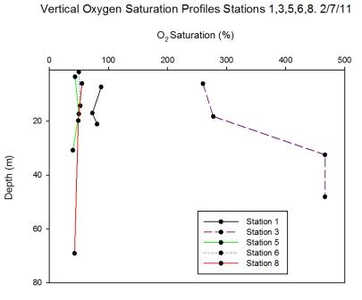
Figure 6.31 |
Phytoplankton & Zooplankton
Analysis
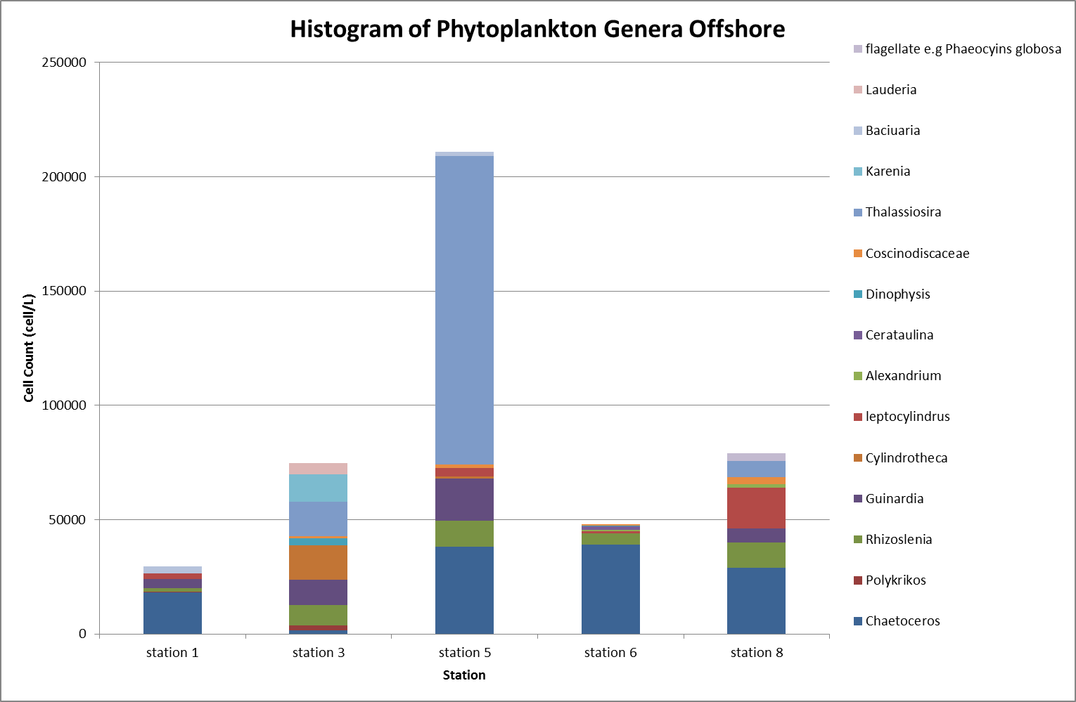
Phytoplankton
|
The highest
abundance of phytoplankton was recorded at station
5, with 211000 cells l-1, the most
abundant phytoplankton was the Thalassiosira genus with
135000
cells l-1 (Figure
6.32). The Thalassiosira are a wide spread
diatom that can be found throughout the world’s
oceans. The high abundance at station 5
could have been due to the depth - the shallower water meant the seabed forced
the thermocline up to the surface, allowing the
nutrients from the deeper cold water to be evenly
distributed throughout the water column and utilised to a greater extent
by photosynthetic organisms in the eutrophic zone.
Station 5 was also a stratified station with
corresponding high levels of chlorophyll that
suggested that the station was recently mixed and
nutrients freshly available; other areas that have
been stratified for longer had become nutrient depleted
in the surface as
the nutrients are rapidly used by surrounding
phytoplankton.
The lowest
abundance was recorded nearby at station 6
(48000 cells l-1), an
inshore station, and the dominant genus was Chaetoceros (39000
cells l-1). Chaetoceros spp. were consistently present at all sampled stations
except for station 3 which had only 1700
cells l-1. Station 6 had the lowest
phytoplankton population where the water column was
mixed indicating it was inshore of the frontal
systems - this could have been due to the nutrients having been utilised
throughout the water column.
Figure
6.30 illustrates that phosphate concentrations
were relatively
low.
The samples
from the two offshore
stations (3 and 8) appeared to have the lowest
phytoplankton populations of the sampled stations;
this could have been due to nutrients not being
mixed to the upper water column as the waters are
stratified. This explains why there was a reduced number of
phytoplankton within the sample. Using
CTD
data the chlorophyll maximum can be shown e.g. 20-30m
at station 3 around the point where the water temperature
fell
as the layers of warm nutrient poor water interacted
with the nutrient rich cold water. At this point there
was sufficient
light and heat for photosynthesis from above and
the nutrients were accessible either by minor
diffusion or by plankton migration through the water
column. The chlorophyll maximum at station 8 was around 25m but the chlorophyll levels
were kept low due to predation by zooplankton -
using the CTD data in
Figure 6.30 high
turbidity can be observed, caused by the larger plankton feeding on
the photosynthetic organisms. |
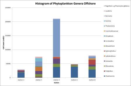
Figure 6.32 |
Zooplankton
|
Knowledge of
variability in zooplankton biomass is important for
understanding the ocean food webs and energy flow in
the oceans; as zooplankton
contribute to the
transport of carbon and nitrogen to the deep sea via
production of faecal pellets and active transport by
vertical migration, which are important components
of the biological pump (Longhurst et al.,
1990). Using information displayed on the computer
in real time from acoustic backscatter intensity
derived from Acoustic Doppler Current Profilers
(ADCPs) and zooplankton biomass from net collected
zooplankton samples, variability in the
distributions of zooplankton biomass are described.
This is
possible as zooplankton are large enough to provide
an image on the ADCP.
The
zooplankton samples collected were taken from areas
that showed high acoustic backscatter in relation to
the surrounding areas.
Sample sites were
also selected based on fluorometer readings, which
indicated areas of high chlorophyll concentrations
at various depths.
This allowed
comparisons of chlorophyll concentration with
zooplankton biomass. All zooplankton samples were
collected from stations where physical data from the
CTD, chemical and biological (phytoplankton) data
from Niskin bottles attached to the rosette system
were all collected.
Samples were collected using a
vertical closing net allowing specific depths within
the water column to be targeted for sampling. All
zooplankton samples were stored in the dark with
formaldehyde added after collection to preserve the
sample.
As seen in
Figure 6.35 the
highest abundance of zooplankton was measured at
stations 3 and 8: 1613 m-3 and 1103 m-3,
respectively. The dominant species at both of these
stations were hydromedusae, 728 m-3 at
station 3 and 467 m-3 at station 8. The
phytoplankton data obtained (Figure
6.32) may explain the higher numbers of
zooplankton at station 3 and 8.
Stations 3 and 8 have different
secondary dominant species; station 3 has decapod
larvae and at station 8 copepods are the second
largest group recorded.
As zooplankton feed on phytoplankton
in areas of well mixed coastal waters, with larger
communities of phytoplankton more zooplankton can be
supported. In this data the larger zooplankton
samples collected were situated further offshore,
this could be due to the chlorophyll maximum at
depth and the development of thermocline (Figure
6.9). Nutrients were constantly replenished from
deeper waters, the phytoplankton were able to grow
thus providing a food source for the zooplankton.
This can be seen in the CTD data as the fluorometer
reading at station 8 shows a minor increase at a
depth of 20m, however there is a large amount of
turbidity which could possibly be zooplankton which
feed on the phytoplankton keeping the chlorophyll
levels low.
At station 5, the zooplankton were
sampled at two depths: 0-15m and 15-30m. High
chlorophyll concentration throughout the water
column suggested that the station may have been
recently mixed allowing the chlorophyll
concentration to rise in response. However the
recent increase in levels of irradiance (http://www.metoffice.gov.uk/climate/uk/anomalygraphs)
may have caused stratification of the water column
with a shallow steep thermocline. High levels of
acoustic backscatter were also observed. For these
reasons two samples were taken from either side of
the thermocline; to study any differences in
zooplankton compositions. From 0-15m station 5 had a
larger number of hydromedusae present (239 m-3)
with a smaller number of copepods (144 m-3),
whereas at 15-30m station 5 was dominated by
copepods (167 m-3). It could be suggested
that this is due to the different communities of
phytoplankton at the thermocline allowing for
different niches for individuals to develop within.
Station 1 is situated at Black Rock
near the mouth of the Fal estuary, there is a low
amount of phytoplankton recorded at this station (Figure
6.32) although there is a high chlorophyll
concentration (Figure
6.2). This could possibly be due to
phytoplankton cells having high chlorophyll content
but are few in number therefore unable to support
high zooplankton abundance.
|

Figure 6.33 - Teleost
Egg photo from zooplankton sample
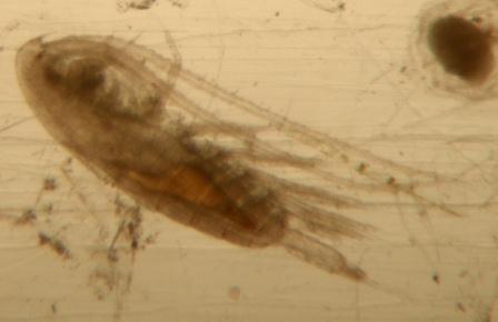
Figure 6.34 - Copepod photo from zooplankton sample
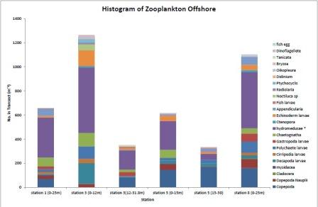
Figure 6.35 |
Comparison of phytoplankton and zooplankton
populations in the estuary and offshore
In the estuary the vast majority of phytoplankton were found
to be diatoms, with a few other forms present. The main
species of diatom sampled were Chaetoceros. This species
was also observed in the offshore sampling, but in smaller
numbers, in addition to many other diatom species that were
sampled in similar sized numbers (Thalassiosira,
Cylindrotheca, Leptocylindrus). Offshore a large number of
dinoflagellates were recorded in addition to diatoms; this
could have been due to the environment being more osmotically
stable with stratified environments, unlike in the estuary,
creating a greater number of niches for organisms to fill
and allowing dinoflagellates to grow where diatoms cannot as
they can use their flagella for motility to obtain
nutrients.
The zooplankton sampled in the estuary and offshore show a
large variation in population composition; the estuarine
zooplankton community had a very high proportion of copepods
and copepod nauplii possible due to a greater tolerance of
changing salinities compared to the zooplankton found
offshore. Offshore zooplankton are less tolerant of changing
environments, as they are used to a more stable environment
and so hydromedusae numbers were much greater than those in
the estuary.
Chlorophyll Analysis
|
The
chlorophyll measurements from the samples collected
reflected the general characteristics at the different
stations and the fluorescence readings on the
CTD profiles.
Stratified stations 3 and 8 (Figure
6.36) show a distinctive
increase in chlorophyll l-1 just beneath the thermocline (shown by comparison to the CTD
profiles). The greatest chlorophyll concentration was
at station 3 with a concentration of 25mg l-1 at 32m.
Both stations show a decline in chlorophyll after
the peak as depth increased. Results at station 5,
which was also stratified,
suggested recent mixing within the surface water as
there was no distinct increase in concentration surrounding
the thermocline. The thermocline was also much weaker
compared to stations 3 and 8. Mixed stations 6 and 1
showed an gradual increase in chlorophyll with depth.
|
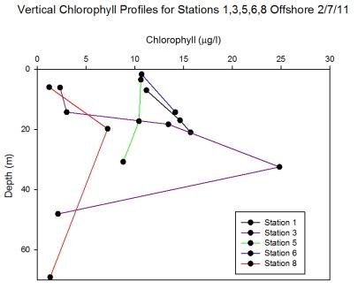
Figure 6.36 |
Conclusion
The offshore data reflect the concept of a frontal system
around half a mile to a mile offshore. ADCP data show
positions where the front was crossed to be between the
27-33m depth contours. The stratification parameter reflects
the position of each station regarding the front well.
Stations offshore of the front reflect a stratified water
column with warm water above colder water and a distinct
thermocline, just beneath which is where the chlorophyll
tends to reach a maximum value as nutrients become available
to phytoplankton residing in the euphotic zone. Mixed
stations show higher chlorophyll values throughout as the
chlorophyll is well mixed throughout the water column as
nutrients are freely available. Nutrient data follows an
expected trend with depth; biomass in the upper water column
causes depletion near the surface of silicon and phosphate.
Offshore the nutrients remain higher beneath the thermocline
where chlorophyll is low as phytoplankton are unable to
utilise nutrients because the light levels are too low at
depth. Offshore the levels of dissolved oxygen tend to be
much higher than inshore with an increase below the
thermocline where biological activity is limited. At the
inshore stations oxygen has a more homogeneous distribution
in the water column due to physical processes mixing the
water column. Surface fluorescence data is high at most
stations but are particularly high at stations near the
front e.g. 5 and 6 reflecting the frontal conditions
providing ideal conditions for phytoplankton blooms, but the
sampling was not fine enough to draw firm conclusions about
how phytoplankton distributions vary across the front.
|
GeoPhysics
    |
Introduction
The aim of this survey was to compile a habitat map from
sidescan sonar interpretation and the use of direct
sampling to gain biological information.
Habitat maps allow
the wide scale geology and present day sedimentary processes
to be determined and understood (Laban 1998). This
understanding of the seabed structure and distribution is
vital to enable effective management of the impact of human
activity and climate change on ecosystem form and function.
Habitat mapping is a powerful tool, allowing comparison of
sites; therefore a global view on the variety of habitats
can be gained and areas important for conservation of
species can be identified. Jordan et al. (2004)
mapped the Kent Group of islands,
south-eastern Australia. This habitat mapping generated a
capability to define the boundary and size of potential MPA.
The Fal estuary is a Special Area of Conservation (SAC) accredited
by the Joint Nature Conservation Committee (JNCC). One of
the reasons for this status is due to the Annex 1 habitat
‘sandbanks covered by water all the time’. Within this
classification the JNCC has made a specific comment on the
importance of the extensive areas of maerl gravel (dead and
alive maerl) which extend throughout the Carrick Rhoads and
Falmouth Bay. The JNCC recognises the importance of maerl
beds due to the diversity of species living among these beds
and the general scarcity of this habitat in UK waters. (www.defra.gov.uk)
The geophysical sidescan survey was undertaken on
L. C. Grey
Bear. Using a sidescan towfish a selected area was first
surveyed, followed by grabs being undertaken at interesting
sites using a Van Veen Grab. Video survey was also used in
order to ground truth the data from the sidescan sonar and
to confirm that areas of uncertainty were suitable for taking a
grab. The habitats present between Pendennis Point, Black
Rock and Falmouth Harbour were surveyed and the findings
were presented on a poster and are described below on this
website.
Trimble Hydropro software was used to create the desired
track for survey following consultation of WGS84 Admiralty
charts. This software was used in conjunction with the
vessel’s GPS in order to provide the skipper with
information about how far port or starboard the vessel was
from the planned track and the course could then be adjusted
accordingly. After the initial survey, the grab sites were
plotted and the ship could navigate to them accordingly.
During adverse
weather conditions, the captain would orientate bow or stern
to the wind as appropriate in order that the grab could be
completed as safely and comfortably as possible. Weather
conditions for this survey are shown in Table 7.1
| Date |
6/7/2011 |
| General Weather |
Bright
and sunny morning, deteriorating to cloudy and rainy
afternoon.
|
| Visibility |
Clear morning, deteriorating slightly in the
afternoon |
| Sea State |
2-5 |
| Cloud Cover |
55% |
| Wind Speed |
15.11 |
| Wind Direction |
SW |
Table 7.1
| 6/7/2011 |
Tide Times GMT |
Tidal Height
(m) |
|
Low Water |
0244 |
0.6 |
|
High Water |
0832 |
4.8 |
|
Low Water |
1459 |
0.8 |
Table
7.2 |
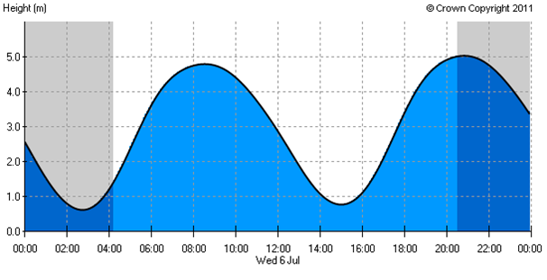
Figure 7.1. Tidal curve for
06.07.2011 |
The three transects undertaken on the
survey are shown in Figure
7.2 and Table 7.3. A fourth transect was also completed,
however due to technical difficulties the record was not
printed; therefore no further reference will be made to this
transect. All three grab sites sampled are also specified in
Figure 7.2. Two video
transects were completed which are shown in
Figure 7.2, an attempt
to video at the first grab site (32011.71N, 182909.50E) was
made, however weather conditions were poor rendering
the footage unsatisfactory for viewing.
|

Figure 7.2 |
|
Transect Number |
Start time (GMT) |
End Time (GMT) |
Start Position |
End Position |
|
1 |
08:54 |
09:08 |
31644 N
182936 E |
32222 N
182252 E |
|
2 |
09:16 |
09:27 |
33002 N
182419 E |
31657 N
182999 E |
|
3 |
09:32 |
09:47 |
31716 N
1830334 E |
33250 N
182370 E |
Table 7.3 |
Sidescan Sonar
The sidescan
system consists of three components: a towfish, a
transmission cable and the topside processing unit. The
towfish was lowered into the water off the stern of the
boat as the area to be surveyed was reached. The towfish
was then transmitting when we entered the survey area. The
towfish was then towed behind and below L.C Grey Bear with
the vessel heading as steady as possible to prevent the
image blurring. The towfish maintained a constant depth
due to the length of the transmission cable.
The
towfish has an acoustic transducer which sends out a wide
angle pulse, this wave then propagates across the seabed.
Every sonar pulse is one line of information as soon as the
pulse is sent the tow fish then ‘listens’ for an echo, this
is called backscatter .This information then gets passed
along the transmission cable. The sidescan sonar system then
displays the intensity of the sound scattered back to the
towfish from the seafloor; the data received was displayed
in real time on a laptop computer screen on the deck of L.C
Grey Bear. This allowed us to detect any objects or
bedforms on the seafloor. The sidescan sonar works based
on the first law of reflection which states that
the
incident ray, the reflected ray, and the normal all lie on
the same plane. Because this only applies to perfectly
smooth surfaces, backscatter is created.
Whilst watching the screen we were able to view the
backscatter data and discuss how the properties of the
seabed are what determine the strength of the backscatter
echo. Rock, gravel, coarse sand and wood are better at
reflecting so they create more backscatter and are therefore
recorded as darker areas than soft muddy sediments; which
produce less backscatter, so appear lighter in colour on the
sonar record.
We also discussed how the angle of the seafloor slope
influences the backscatter; slopes facing away from the
transducer appear dark, and slopes facing towards the
transducer appear paler. Another feature of the sidescan
system we noted whilst carrying out the survey was how a
3-dimensional quality can be achieved by acoustic shadows
(Figure 7.3). These acoustic shadows occur alongside
areas that stand out or dip down in the sea-floor; these are
very useful for indicating the shape and nature of the
mound/groove/bed-form.
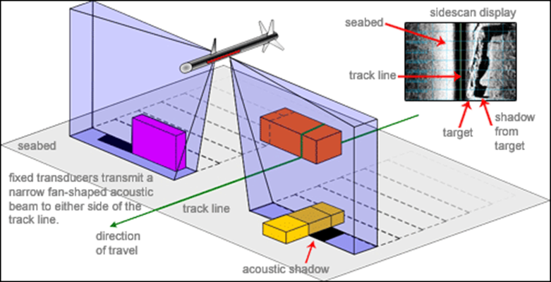
Figure 7.3 Sidescan theory |
The operating frequency on the
sidescan sonar can be altered depending on the resolution
and swath required. A low frequency, such as 100 kHz, will
give a wider swath width but the resolution will be lower.
This is useful for surveying large areas. A higher
frequency, such as 500 kHz, will give better resolution but
a narrower swath width. An even higher frequency of 2.5 MHz,
for example, can be used for a really well defined image;
however this will significantly lower the swath range, so
would be used in small sites. This survey was operated at
110 kHz.
Swath systems, such as sidescan sonar, are most likely to
provide the best high-resolution maps, particularly over
wide areas. They provide information on sediment texture and bedform structure and allow dynamic processes (e.g. sediment
transport) to be deduced. Disadvantages associated with
swath systems are their high costs and the need to have
skilled interpretation. In addition, the output often
requires considerable post-processing time and expense to
obtain appropriate classifications (Kenny et al.,
2003).
Limitations
There are a few
limitations with sidescan sonar. One is the interference
produced by the ship’s echo sounder which produces sharp
marks on the sidescan sonar when running at high frequency.
Other sources of interference include other sonar sources as
well as dolphins. Dolphins use a frequency of 400nm for
hunting and for communication they have use a frequency of
100nm which is at the lower end of sidescan and produces
weird traces.
Another problem
is due to the fact that the sidescan beams widen with
distance from the tow fish and so objects may merge if for
example there were two closely placed objects from the
perspective of the tow fish it would look like one, for
example seaweed appears like single white lines
rather than many plants (see
Figure 7.4).
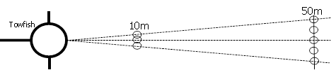
Figure 7.4 |
Lastly is the
uncertainty with the sidescan, when analysing bedforms can
only be suggested and the scan only gives an indication of
what the bed could be formed from (substrate/bedrock).
This emphasises the need for ground truthing by taking grabs
and video footage.
Grabs
Grab 1
| Time |
1033GMT |
| Northings |
23011.71 |
| Eastings |
182909.5 |
|
Sediment Description |
Fauna and Flora |
| Sediment was made up of
mainly coarse and very coarse sand, 70% of
which was retained in the 2mm sieve and 25%
in the 1mm sieve. Rocks and pebbles made up
the remaining 5% and were retained within
the 10mm sieve. Sediments also contained
broken Mollusca shells and dead maerl. |
Live maerl
Hermit crabs
Long
clawed porcelain crabs
Kelp
Rock with
attached keel worms, pink coralline algae,
green algae, pink ray limpets |
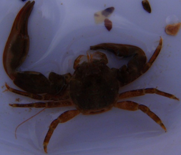
Figure 7.6 - Long Clawed
Porcelain Crab |
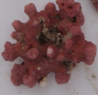
Figure 7.7 - Live Maerl |
Table 7.4 |
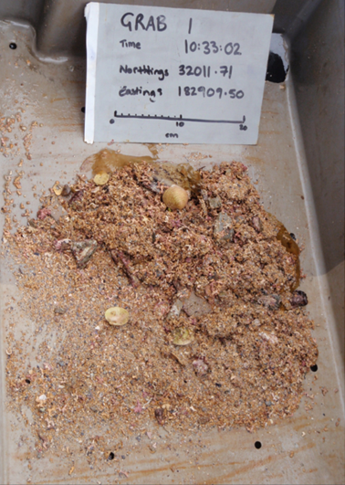
Figure 7.5 |
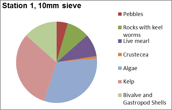
Figure 7.8 |
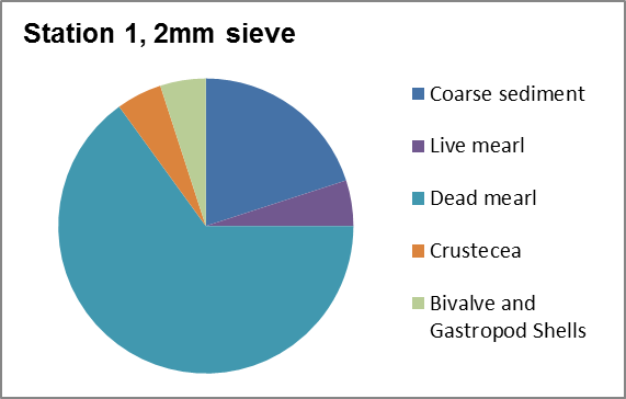
Figure 7.9 |
Maerl is a free living, calcified, coralline
red algae. Maerl beds are composed of either living or dead
unattached maerl which form branching and interlocking
structures (Birkett et al. 1998). Maerl beds form in
areas without high levels of siltation, as this leads to
smothering and burial of the maerl which will reduce
photosynthesis, laboratory experiments show that smothering
by fine sediment and lowered oxygen concentrations are
particularly damaging to maerl algae (Wilson et al. 2004).
Maerl is an important habitat for numerous species and thus
support high biodiversity and high trophic group diversity (Barbera
et al. 2003).The main ecological role for maerl is to provide
shelter for animals and attachment for plants (Castriota
et al. 2005).
Grab 2
| Time |
1121GMT |
| Northings |
32339.25 |
| Eastings |
182695.08 |
|
Sediment Description |
Fauna and Flora |
|
No sediment was
recovered in the grab however the fur
bellows hold fast was attached to a 250mm
rock. |
Furbelows
Sugar kelp
Irish moss
Red and Brown algae
Painted and Grey top shells
Whelks
Snakelocks anemone
Porcelain and Edible crabs
Squat lobsters
Barnacles
Cowrie |
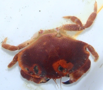
Figure 7.11 - Edible Crab |
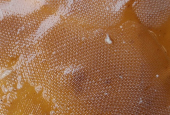
Figure 7.12 - Bryozoa |
Table 7.5 |
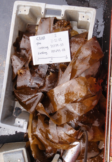
Figure 7.10
|
Furbelows kelp
Phylum:
Orchrophyta
Class:
Phaeophyceae
Species:
Saccorhiza polyschides
Habitat
description: Saccorhiza polyschides grows from
extreme low water springs to a depth of 35 m. It normally
attaches to rocks but is occasionally found loose-lying on
small stones or shells. It can form dense stands in
sheltered areas and can tolerate strong currents.
Description:
Saccorhiza polyschides
is kelp species with a distinctive large warty holdfast and
a flattened stipe with a frilly margin. The stipe is twisted
at the base and widens to form a large flat lamina, which is
divided into ribbon-like sections. The species is an annual,
and very fast growing. It is opportunistic and colonises
available hard substrata in the sublittoral
(www.marlin.ac.uk).
Sugar Kelp
Phylum:
Chromophycota
Class: Phaeophyceae
Order:
Laminariales
Species:
Saccharina
latissima
Habitat description: Sometimes
found in littoral rock pools but more commonly in the
sublittoral below 20m anchored to rocky substrate using a
large holdfast. Widespread global distribution in temporal
waters
Description: Can grow up to 4 m long, attached
to rock by strong cylindrical stipe. Long, leathery,
unbranched blade about 15cm wide without a midrib. Blades
are flat but wrinkly with wavy margins.
Grab 3
| Time |
1209GMT |
| Northings |
33013.9 |
| Eastings |
182538.2 |
|
Sediment Description |
Fauna and Flora |
|
Sediment was made
up of mainly small pebbles and coarse sands,
50% of which was retained in the 10mm sieve,
30% in the 2mm sieve and 20% in the 1mm
sieve. Sediments also contained broken
Mollusca shells and dead maerl. |
Brown algae
Sand mason worms
Grey and Flat
top shells
Cowries
Brittle star
Crabs Live
maerl
Brittlestar
Towershell
Rock with
attached keel worms, pink coralline algae, platyhelminthes
|
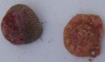
Figure 7.14 - Grey and Flat Top
Shell |
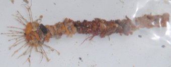
Figure 7.15 - Sandmason Worm |
Table 7.6 |
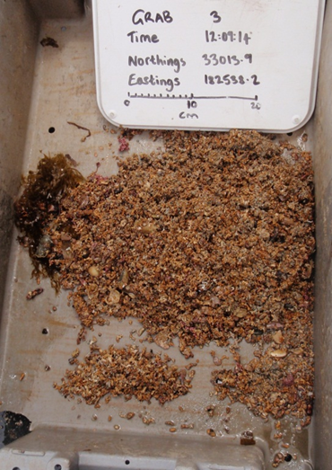
Figure 7.13 |
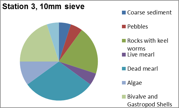
Figure 7.16 |
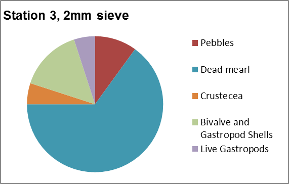
Figure 7.17 |
Video Analysis
|
The video
trawls show that the habitat surveyed with the video
was a sandy/shingle bottom, with a third to a
quarter covering of empty larger shells. Red (for
example Dudresnaya verticillata) and green seaweeds
and some kelp covered approximately a tenth of the
seafloor. There were occasional large features
covered in kelp and rhodophyta. As the long trawl
following the second grab progressed more of the
seabed became covered in maerl and occasional shoals
of juvenile fish were observed (maerl is known as an
important nursery ground for juveniles).
|
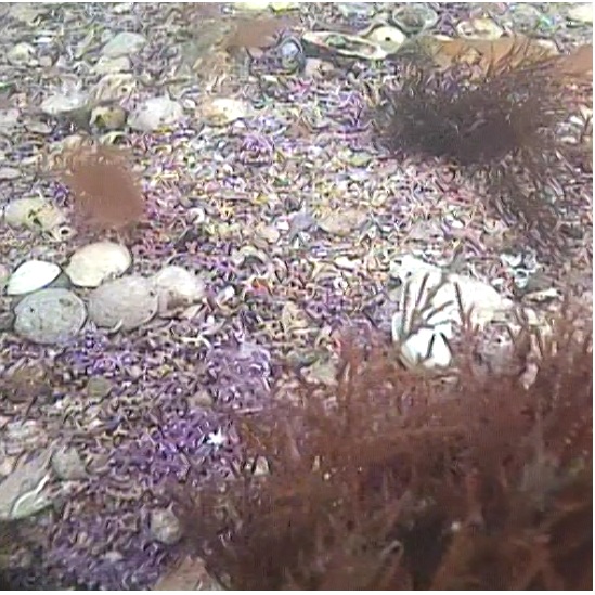
Figure 7.18 |
Conclusion
Interpretation
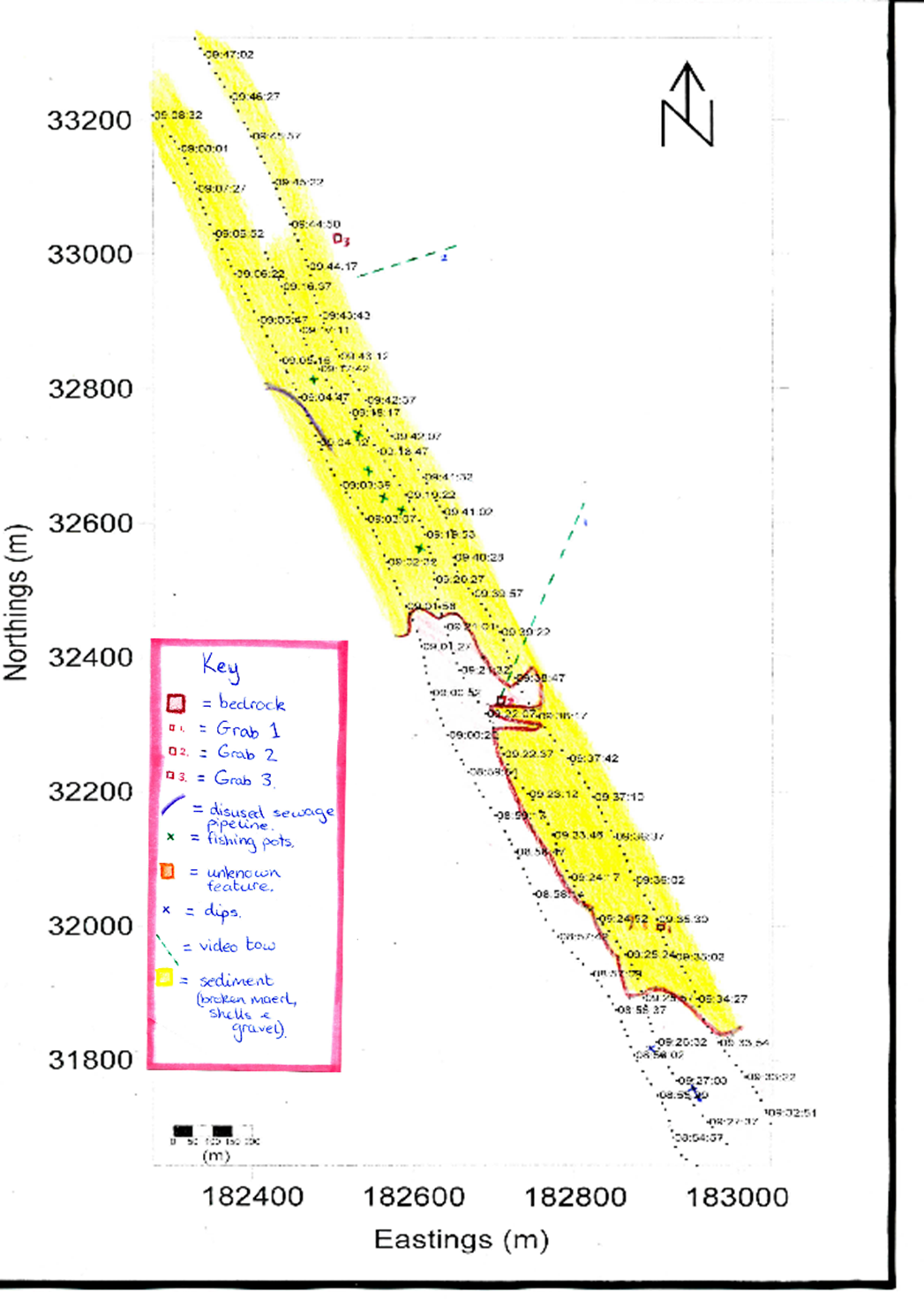
Figure 7.19 |
|
The most Northerly point of the transect (33295N, 182410E)
consists of sediment including broken maerl, shells and
gravel, as indicated by grab 3 which was taken nearby (Figure
7.19). This
bed type persists in a South East direction, until position
32490N, 182480E. Here, the bedform is divided and sediment
is present only in the East of the tracks. In the West a new
bedform exists; a mix of bedrock, boulders, gravel and
seaweeds. A decision was made to sample at the division
between two substrate types, grab 2. This made it possible
to see the transitional species that inhabit this area. This
division between sediment and bedrock runs from 32490N,
182640E to 31895N, 182895E, with some gullies and peninsulas
extending from the main body of the bedrock.
Grab sample 1 was taken at 32011N, 182909E in an area
that had been identified on track 3 as having sidescan
signatures for fine sediment. To achieve a contrast between
grabs and understand the variations of fauna and flora found
between sediment and rock substrates.
Key notable features in the sediment include lobster pots,
which are absent in the bedrock. At point 32800N, 182440E
and extending to 326710N, 182500E lies what is likely to be
a pipeline from the disused sewage treatment facilities on
the nearby shore.
At the extreme South East end an area exists from; 31860N,
182840E to 31770N, 182865E across all three transects.
Here, bedrock dominates with no presence of sediment and
three prominent dips have been identified on the sidescan
trace. Pythagorean equations have shown that the depth and
length of these differ as indicated above. However when
analysing the sidescan trace one must bear in mind that
from different angles the same bedform may appear different.
This is one of the limitations of sidescan: the nature of bedforms and substrate may only be suggested and grabs are
required to provide verification. This verification process
is known as ground truthing. Grab 3 was taken from the same
sediment type as grab 1 but at some distance away to allow
analysis of any spatial gradients in flora and fauna that
may exist. This can only be done because the type of
organisms that were sampled move at a negligible rate with
comparison to the progress of the surveying vessel. |
|
|
Discussion of Further Possible
Investigation |
|
Further
investigations in the estuarine system that spring from our
findings may include investigating how the mussel farm on
the Fal Estuary affects the chemical and biological
parameters in the estuary. Our data may have been influenced
by the mussel farm on several occasions including
phytoplankton and oxygen concentrations. The phosphate
additions in the estuary, presumed to be from agricultural
practices, sewerage outputs and possible mine drainage,
could be monitored to observe any change over time and how
this relates to current practices at potential input sites.
Phytoplankton and zooplankton populations in the estuary
could be further investigated and compared to other
estuarine systems in the area such as the Helford Estuary
and up Restronguet Creek.
In the offshore
system, the frontal systems could be further investigating
by finer sampling closer to the front – this would provide
more detailed data on phytoplankton distributions across the
system and how this varies to offshore data generally. Time
series sampling of the front over the course of the year
would investigate how the front moves.
Geophysical
surveying and habitat mapping in the same area that we
sampled could be repeated over time to give a time series
that could be used to show how the habitat varied,
particularly with reference to the maerl as an important
long living organism of conservation value. The area that we
sampled in was close to the outer harbour wall, parts of
which are currently disintegrating, and contain various
substances likely to cause pollution. |
|
References |
|
|
|
Barbera C. (and 17
others) 2003. Conservation and management of
northeast Atlantic and Mediterranean maerl beds.
Aquat. Conserv.Mar. Freshwat. Ecosyst: 13, 65–76
|
|
Birkett D.A. Maggs C.A. &
Darling, M.J. 1998. Maerl, (Volume V) An
overview of dynamic and sensitivity characteristics
for conservation management of Marine SACs.
Scottish Association for Marine Science (UK Marine
SACs project). 116
|
|
Boyer I.C. Gillespie P.A. Kaspar H.F. MacKenzie A.L. 1995. Effects of mussel aquaculture on the
nitrogen cycle and benthic communities in Kenepuru
Sound, Marlborough Sounds, New Zealand. Marine
Biology: 85:2, 127-136 |
|
Cadee G.C.
1978. Primary production and chlorophyll in the
Zaire River, estuary and plume, Netherlands.
Journal of Sea Research : 12, 368-381 |
|
Castriota L. Agamennone F.
& Sunseri G. 2005. The mollusc community associated
with maerl beds of Ustca Island. Cah.Bio.Mar:
46, 289-297
|
|
Engel C.R. Guillemin M.L. Jacob A.M. Valero M. Viard
F. 2008. Permanent Genetic Resources: Isolation of microsatellite loci from the kelp,
Saccorhiza polyschides
(Heterokontophyta,
incertae sedis)
Molecular Ecology Resources: 8, 406–408
|
|
Huot Y. Babin M. Bruyant F. Grob C. Twardowski M.S. Claustre H. 2007. Does
chlorophyll a provide the best index of
phytoplankton biomass for primary productivity
studies? Biogeosciences Discuss: 4, 707-745 |
|
Jordan A. Lawler M. Halley V. and Barrett N. 2005. Seabed habitat mapping in the Kent Group of
islands and its role in Marine protected area
planning. Aquatic Conservation: Marine and
Freshwater Ecosystems: 15, 51–70
|
|
Kenny A.J.
Cato I. Desprez M. Fader G. Schuttenhelm R.T.E.
Side J. 2003. An overview of seabed mapping
technologies in the context of marine habitat
classification. ICES Journal of Marine Science:
60:2
|
|
Laban C. 1998.
Seabed mapping. Hydro International: 2:1, 4 |
|
Langston W.J. Chesman B.S.
Burt G.R. Hawkins S.J. Readman J. Worsfold P. 2003. Site Characterisation of the
South West European Marine Sites: Fal and Helford
cSAC. Marine Biological Association |
|
Lorder C.T & Reichard R.P. 1981 The dynamics of
conservative mixing in estuaries. Estuaries and
Coasts: 4:1, 64-69 |
|
Mullin J.B. & Riley J.P.
1954. The colorimetric determination of silicate
with special reference to sea and natural waters.
Analytica Chimica Acta:12, 162-176.
|
|
Simpson J.H. & James J.D. 1986. Coastal and
Estuarine Fronts. Baroclinic Process on
Continental Shelves. Geophys. Union: 63-94. |
|
Souchu P. Vaquer A. Collos Y. Landrian
S. Deslous-Paoli J.M. Bibent B. 2001.
Influence of shellfish farming activities on the
biogeochemical composition of the water column in Thau lagoon.
Marine ecology progress series: 218, 141-152 |
|
Vesci A. 2001. Fore-reef
carbonate production: Development of a regional
cencus based on method & first estimates.
Palaeogeology, Palaeoclimatology, & Palaeoecology:
175, 185-210
|
|
Welschmeyer N.A. & Lorenzen
C.J. 1985. Chlorophyll budgets: Zooplankton grazing
and phytoplankton growth in temperate fjord and
central Pacific Gyres |
|
Longhurst A.R. Bedo A.W. Harrison W.G.
Head E.J.H. Sameoto D.D. 1990. Vertical flux of
respiratory carbon by oceanic diel migrant biota.
Deep-Sea Research: 37:4, 685–694.
|
|
Wilson S. Blake C. Berges
J.A. Maggs C.A. 2004. Environmental tolerances of
free-living coralline algae (maerl): implications
for European maerl conservation. Biological
Conservation: 120, 283–293
|
|
Websites Accessed
Accessed:
www.envirogene.co.uk/downloads/casestudies/envirogene_case_fal.pdf
, 7th July 2011
Accessed:
www.westcountrymussels.co.uk, 7th
July 2011
MarLIN
- Marine Life Information Network [Online]
Available:
http://www.marlin.ac.uk/speciesfullreview.php?speciesID=4284
[Accessed 2011, July 7th]
JNCC – Joint Nature Conservation
Committee [Online] Available:
http://jncc.defra.gov.uk/ProtectedSites/SACselection/habitat.asp?FeatureIntCode=H1110
[Accessed 2011, July 7th]
Tri tech
innovative underwater technology. [online]
Available:
http://www.tritech.co.uk/products/info/products-info-sidescan_sonars.htm
[Accessed 2010, November 23rd]
|
|
Disclaimer: The ideas
expressed in this website are those of the group and do not
reflect those of the University of Southampton or the
National Oceanography Centre (NOC).
|
|