

Introduction
Methods - SideScan
Methods - Grabs
Methods - Video
Results - SideScan
Results - Grabs
Results - Video
Discussion
Conclusions
Physical - Methods
Physical - Results
Chemical - Methods
Chemical - Results
Chemical - Discussion
Biological - Methods
Biological - Results
Biological - Discussion
Conclusions
Methods
Physical - Methods
Physical - Results
Chemical - Methods
Chemical - Results
Discussion - Physical/Chemical
Biological - Methods
Biological - Results
Biological - Discussion
Conclusions
Note: Click on figures to enlarge them
| Location | The Group | Habitat Mapping Case Study |
| Estuarine Case Study | Offshore Case Study | References |
In summer 2011 we had an educational field trip to Falmouth, UK, to explore the Falmouth bay region from a marine scientist point of view. The choice of location was not accidental, as there are a lot of possibilities to research the Fal estuary looking at the levels of pollution and the effects disturbance has on important aquatic habitats of the coastal and estuarine area.
The Falmouth Bay region is located on the south coast of Cornwall and has inputs of several rivers, the main two being Fal and Helford. Both of their estuaries are rias - flooded river valleys that formed as the sea level rose at the end of the last Ice Age. The Fal estuary is relatively deep (up to 34m in the main channel) and large, consequently, associated with a lot of activity from the docks and a number of sailing clubs. The main body of the estuary is called Carrick roads and one of our surveys took place in that location. There are numerous creeks flowing into the Carrick Roads, however overall input of freshwater into the estuary in relatively low. Tides, however are quite strong, with a range up to 4.5m and extending inland up to Truro.
Reflecting the underlying geology of the Fal, the sediments and catchment are affected by the Carnmellis granite and surrounding metamorphic rock to the west of the estuary. There is only limited amount of sediment deposition in the outer estuary demonstrated by the fact that the Carrick Roads have been very stable over the last 200 years (IECS, 1996). The industry surrounding the region has had a profound effect on the sediment composition, most notable being major silting impacts in the upper estuary and the saltmarshes resulting from china clay wastes from the St Austell area. A significant impact on inputs to the Fal region, particularly within the Carnon river valley, occurred from the mining of metalliferous deposits in the surrounding area. While there is little mining industry still active to contribute to pollution in the region, the residual drainage from abandoned mines continues to affect the sediment geochemistry as the contaminated sediments are being distributed throughout the estuary.
The Helford estuary is significantly smaller and less industrially developed than the Fal estuary. The short open coast between Falmouth and the Helford River is varied and includes exposed open cliffs and hard rock headlands with small beaches and brackish lagoons. The coastline also includes the main tourist area with plenty of hotels and the frontage modified by the structures protecting it against erosion. Sedimentary Devonian carboniferous rocks to the west and south have the most influence the catchment of the Helford estuary, as well as granite to the north, which had been mined until 1993. Unlike the Fal, little pronounced effect of industry is observed on the sediments of the Helford.
The importance of Fal and Helford estuaries and the open coastline is associated with commercial and recreational activity as well as the internationally recognised significance the natural environment. The habitats of interest include: saltmarshes, important for bird populations; maerl beds and sea-grass meadows, that provide nursery grounds for juvenile fish and benthic fauna; mussel beds.
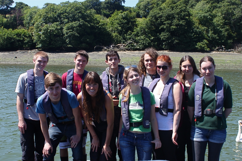
Figure 1: Group 5, Falmouth, 2011
We are a group of 3rd year students, studying at the School of Ocean and Earth Science, University of Southampton, UK. The Falmouth field course detailed on this website is a third year module SOES3018. The group can be split into two different degree programs:
- Marine Biologists: Alicja Dabrowska, Alec Ginns, Sarah-Emily Hemsley, Jack Hollins, Reece Merk, Marija Nilova, Matt Richardson.
- Oceanographers: Jenny Armitage, Dave Lake, Josie Mahony.
The aim of this field course is to collect and analyse biological, chemical and physical data about the Fal Estuary and the surrounding area; and then to compare it to previous studies of this region. The study site is especially important as Falmouth Bay is a Special Area of Conservation and numerous projects regarding habitat mapping are run there; meaning that any data collected is used to further the knowledge about the area.
We had almost a fortnight to perform three surveys of the estuary and the offshore area, collected a large amount of biological, physical and chemical data, which was then analysed during lab sessions, related our data to the research that had already been made in this region and produced a website, where the results of our long hours of work are summarised and presented in a clear and concise way.
A survey was conducted at Carrick Roads within the Fal estuary, to investigate the mechanical disturbance caused by MV Mitera Marigo wreck on the sediment and benthic species composition.
The MV Mitera Marigo was a Greek cargo ship carrying 12, 100 tons of iron ore to Rotterdam until a collision with a German freighter in 1959 which led to a change in direction to Falmouth. The ship was moored in the Carrick Roads and refused help from the local tugs as they would claim salvage, however, it sank soon after as it had taken in too much water. In 1962 the bulk of the cargo was removed and the wreck was flattened with explosives to eliminate the navigational hazard.
The current location of the wreck (50.172106 N; 5.036538 W) was first established from an Admiralty Chart and confirmed with a side-scan, which was performed during the survey. The side-scan was also intended to determine whether any bedforms were present in the area surrounding the wreck and estimate the seabed roughness. Two grab samples were taken to assist the interpretation of the side-scan and to identify the benthic species composition. The samples were analysed using a stack of sieves with mesh sizes of 10mm, 2mm and 1mm. As an alternative way to look at the seabed surface an underwater video camera was deployed in a shallow region of the survey area and the material filmed was used to supplement the data obtained from the side-scan and the grab samples.
A tow fish attached to a 3.6m line and was deployed from 'R.V Grey Bear' to produce a subsurface Dual frequency Analogue Side Scan at 100 KHz of the marine environment, between 08:50:40 - 09:22:45 AST on the 29th June 2011. A sidescan was carried out along 4 lines, which had 100m spacing (See Table 1). The conditions were favourable for conducting a side-scan, a Calm Sea State, UV index 6/11, sunny intervals with a temperature of 15°C. The tides (See table 2) were nearing LW and Winds were 11-14mph in a WNW direction when we performed the sidescan, with a 5⁄8 cloud cover throughout day.
| Line | Start | End | ||||
|---|---|---|---|---|---|---|
| Latitude (N) | Longitude (W) | Time (GMT) | Latitude (N) | Longitude (W) | Time (GMT) | |
| 1 | 50°17.938 | 005°03.212 | 08:50:40 | 50°17.686 | 005°03.644 | 08:54:40 |
| 2 | 50°17.779 | 005°03.536 | 08:55:42 | 50°16.744 | 005°02.052 | 09:01:42 |
| 3a | 50°17.739 | 005°02.284 | 09:02:44 | 50°17.908 | 005°03.141 | 09:08:42 |
| 3b | 50°17.512 | 005°03.480 | 09:09:42 | 50°17.725 | 005°02.853 | 09:14:43 |
| 4 | 50°17.343 | 005°03.419 | 09:18:42 | 50°17.533 | 005°03.454 | 09:22:45 |
| Tide | Morning | Evening |
|---|---|---|
| HW (High Water) | 04:28 (4.4m) | 16:51 (4.7m) |
| LW (Low Water) | 10:52 (1.2m) | 23:19 (1.2m) |
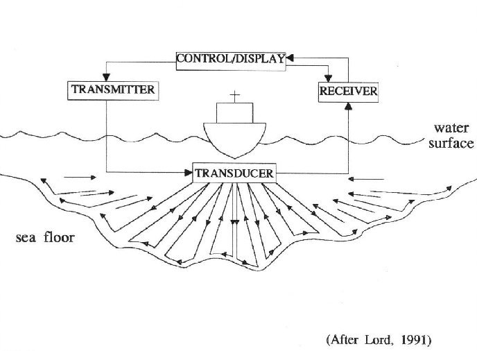
Figure 1: How sidescan sonar works
The towfish had approximately a 70m swath (varied between 67m and 72m depending on the depth of the water column) and a layback of approximately 3.12m (depth data of the towfish was not available, therefore an arbitrary depth of 1.8m was chosen to calculate the layback). The distance from the GPS receiver to back of the boat was 4.9m.
The frequency from the Side Scanner emits a pulse, which is either absorbed or reflected back to the transmitter known as backscatter (Figure 1). A 100kHz signal is at the lower end of the frequencies that can be used on a Scanner (higher ranging up to 600kHz). Applying a lower frequency increases the range (i.e. up to 200-300m; Figure 2) which is ideal for detecting larger objects, or targets e.g. wrecks, however consequently it loses some resolution.
The signals retrieved by the scanner were relayed on to an on board computer which quantified and displayed the varying levels of backscatter, in this case in a black and white colour spectrum. The darker images represent higher reflectance, which indicates denser material i.e. harder sediment types, objects, elevated bed forms. Lighter/white images represent the less dense sediment types or shadows of objects and bedforms depressions. As the computer output was printed and displayed the Latitude and Longitude was recorded of any main areas of interest to then return to with the Van Veen grabs and videography. Four transects were taken (Table 1), however transects 3, 3a and 4 were obstructed by a large moored ship, 'Norman' which was situated at the crossroads mooring station.
A Van Veen grab, with a grasp size of 0.5m2 was deployed to obtain benthic samples to ground truth the features noted from the side scan at 2 locations (See Table 3).
| Grab 1 | Grab 2 | |
|---|---|---|
| Time (GMT) | 10:45 | 12:27 |
| Depth (m) | 23 | 10.5 |
| Latitude (N) | 50°17.001 | 50°17.886 |
| Longitude (W) | 005°03.097 | 005°03.280 |
Sieving occurred once the samples were collected, using 3 different sized meshes (10mm, 2mm and 1mm). A bilge pump was used to wash the sediment and separate the sample. Photos were taken of each sieve (at 30cm set distance) with the grain size card in view.
A video survey was attached to a line and deployed. The images were projected on a screen onboard and recorded. The video provided supplementary data to help identify the true form of the seabed. By utilizing video in addition to the side-scan and Van Veen grab, three different forms of data collection aid to an accurate interpretation, in order to evaluate to our hypothesis.
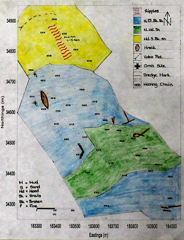
The wreck of the Matiria marigo was surveyed and 4 distinct benthic areas identified and classified as Wd. S. Bk.Sh (Weed, Sand and Broken Shells), M. Wd. Sh (Mud, Weed, Shells) and M. fS. Bk.Sh (Mud, Fine Sand and Broken Shells) on the Habitat Map. In the region labelled as M.fS.bK.Sh. Bedforms with a height of 0.9m and a wavelength of 5.46m could be recognised, as could dredge marks. From the sidescan data it was calculated that the height of the boat was approximately 2.09m, with the highest point being 3.84m tall, which protruding 1⁄4 of the way along the boat. However these may not be accurate results as it was difficult to determine which parts of the wreck were making which shadows on the sidescan. However the sidescan data that we received was limited by the fact that there were equipment issues (the program was not applying TVG on the first track). Also a large ship was moored close to line 3 and many fishing boats and yachts were around, so lines had to be adjusted.
 |
 |
 |
|---|---|---|
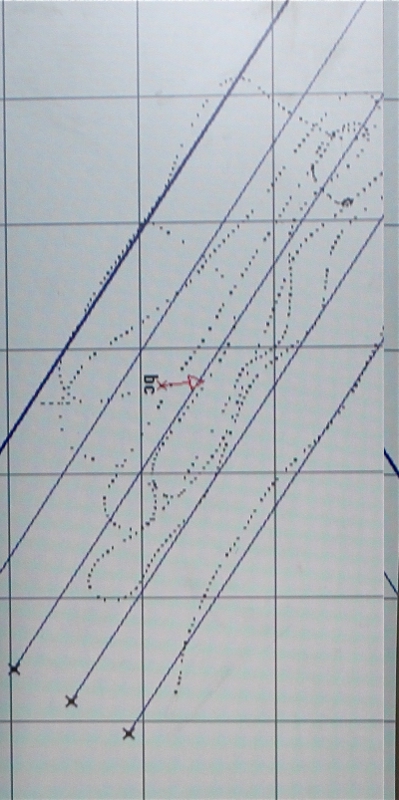
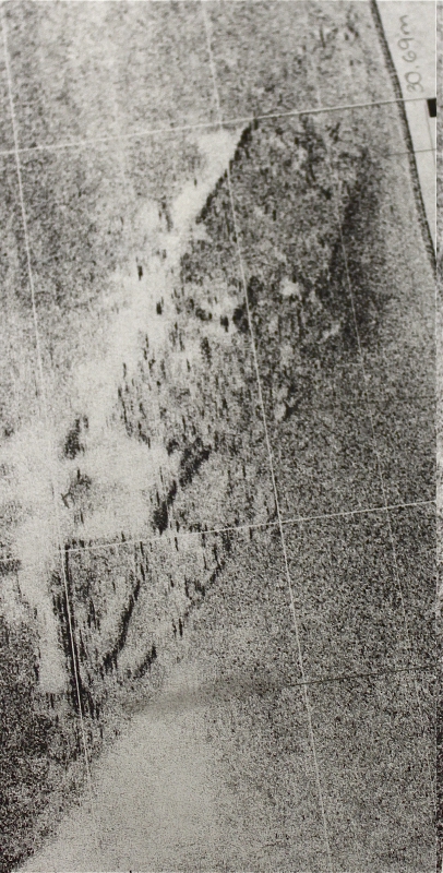
Figure 2: Trackplot for the survey area | Figure 3: The wreck of the Mitera Marigo shown on sidescan sonar | Figure 4: A habitat map for an area in the Fal estuary, constructed using data from sidescan sonar, grabs and a video |
The sample consisted of a thin oxic surface layer (pale yellow in colour) and anoxic layer (dark grey), the sediment was muddy with inclusions of broken mollusc shells and calcareous maerl fragments. Once the sediment had been sieved, in the first sieve (10mm mesh size) the following live species found included broken Porifera spp., Ascidian spp., Megalomma vesiculosum (Tubeworm), Myxicola infundibulum (Tubeworm) and Nereis diversicolor (Ragworm). There were also a few large fragments of dead maerl, bivalve shells and sponge pieces.
The second sieve mostly consisted of bivalve shell fragments and maerl. The majority of maerl (Phymatolithon calcareum or Lithothamnion corallioides) found in this sample was found in the 2mm mesh sieve and the alive to dead maerl ratio was estimated to be about 1:5. Juvenile Sipunculid spp., Trivia monacha (possibly Goldfingia vulgaris) were also found.
In the third 1mm mesh sieve only the smallest maerl and shell pieces were left and no live species were found.
 |
 |
|---|---|
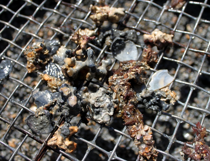
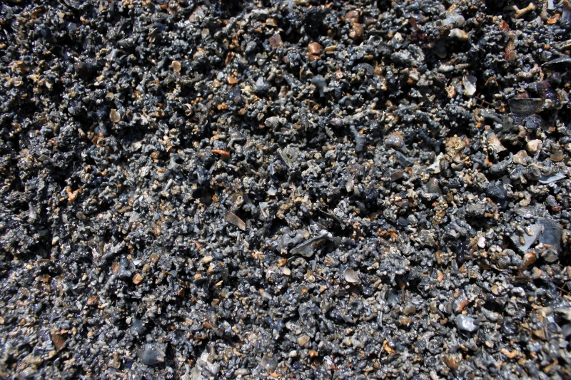
Figure 5: Fraction of grab sample 2 retained in a 10mm sieve | Figure 6: Fraction of grab sample 2 retained in a 2mm sieve, after sieving in a 10mm sieve |
The sediment found in the second grab was slightly more oxic (more yellow sediment present) mixed and slightly coarser than the first. It consisted of mud, sand and small gravel and contained numerous small mollusc shells, and a higher proportion of maerl compared to the first sample.
After the mud was washed out, the 10mm sieve retained numerous juvenile representatives of several polychaete families, such as Phyllodocidae, Terebellidae and Nereididae; clusters of calcareous polychaete tubes (Pomatoceros spp.); fragments of seaweed Fucus serratus and dead maerl (Figure 5). No large shell fragments were present as opposed to the first sample but live gastropod molluscs were more abundant and included Raphitoma purpurea and representatives of Turridae family. The 2mm sieve contained maerl, with alive to dead maerl ratio of about 1:10, and numerous juvenile bivalve and gastropod molluscs (Figure 6).
The 1mm sieve only had fragmented maerl and the smallest mollusc shells.
The benthic area surveyed by the video had weed coverage that varied between 30-60%, uniform broken shells and sand elsewhere. Chlorophyta (green algae) was present but rare and there were high turbidity levels.
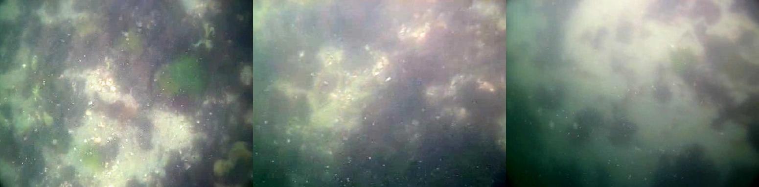
Figure 7: Stills from a video survey of the estuary benthos
Similar physical properties of both grab samples can be determined through a combination of video, sidescan sonar, chart observation and direct grab observational methods. These various methods allowed for direct evaluation of the impact of the presence of a wreck on the benthic environment. It was possible to assume that observed differences in biota were a result of the presence of the wreck, and not due to variation of other physical conditions.
The principle difference in the observed biota was the evidence of sessile filter feeders (Porifera fragments and whole Ascidians) in grab one, in the presence of the wreck. These require hard, stable substrata to adhere to, and also sufficient flow of water to supply enough nutrition to allow for efficient growth and lifecycle completion. Leichter and Witman (1996) observed enhanced growth of sessile filter and suspension feeders attached to subtidal rock walls when compared to those attached to the surrounding seafloor. This was interpreted as a result of the rock walls effectively 'funneling' flow from the surrounding area directly over the 'wall fauna'. Similar dense aggregations of Poriferans and Ascidians have been observed on subtidal rock faces in estuaries in the Southwest of the UK (Barne et al., 1996). The additional height above the seafloor of the wreck may also allow for filter feeders to escape the laminar flow boundary layer found at the sediment/sea floor interface, within which nutrients can quickly become depleted. It is likely that the debris, which was calculated as being higher than 2.09m in places, acted as functional subtidal walls, allowing for the growth of the observed sessile fauna.
Other faunal variation between the two grabs allows us to infer further impact of the wreck. Suspension feeding tubeworms were found only at grab site 1. Although materials for tube construction, such as shell fragments, were observed at both grabs. Suspension feeding apparatus becomes clogged by large amounts of sediment smaller than 2mm, present in each grab (Dough et al., 1999). It is possible that the wreck provides shelter, preventing large influx of particulate matter, or by disrupting the laminar flow of water across the seabed, preventing accumulation of sediment. Deposit feeding Sipunculids were found at grab site 1, while Terrebelid polychaetes, also deposit feeders were found only at grab site 2. The fine grained sediment preferred by most deposit feeders was present at both sites, so the reason for the absence of any Terrebelidae from site 1 is unclear, although competition for resources between the Terrebelid and tube worms may explain this, as both occupy a similar ecological niche, while the smaller Sipunculids may be able to survive on less available food resources.
The variation in gastropod populations between the two sites was determined as not being directly caused by wreck presence, but rather as by the presence of their individual prey items, T. monacha preying on ascidians, both found in grab one, and Turitellid gastropods preying on Terrebelid polychaetes, both present in grab 2.
The variation in benthic fauna observed at the two sites shows that while the wreck has little impact on the physical parameters of the benthic habitat, it does directly provide an alternate habitat in itself. This must be considered when using benthic species as indicators of biotopes, as it shows how there may be great, albeit localised, biotic variation within habitats which may otherwise be identified as uniform.
The aim of the fieldwork, carried out on R.V. Bill Conway, was to develop an understanding of how the Fal estuary acts as a transition zone between the freshwater input and the coastal sea.
A survey was carried out on 02/07/2011, from 7:45 to 14:00 (GMT) on the R.V. Bill Conway. It was a sunny day, with cloud cover between 0⁄8 and 1⁄8, temperature 17-19°C, wind speed 9mph and wave height <0.5m. The tidal predictions for Fal Estuary were: HW at 5:40 (4.8m), LW at 12:11 (0.8m), HW at 17:54 (5.1m) (times in GMT).
Specific areas of interest between the area of freshwater input and the coastal sea were sampled (Table 1), providing physical, chemical and biological observations. The physical observations were salinity and temperature structures, alongside secchi depths and current profiles. The chemical observations were nutrient (Si and P) and dissolved oxygen samples. The biological aspect consisted of samples of chlorophyll, phytoplankton and zooplankton.
CTD provided measurements of temperature and salinity variations with depth. It also had a fluorometer and transmissometer attached. Measurements were taken at pre-determined intervals along the sea to freshwater input transect. In conjunction with the transect data, vertical profiles were taken and Niskin samples were also collected at specific depths (Table 1), subsequent to interpreting the 'down' transect. The CTD had been calibrated before arrival in Falmouth. The aim of using the CTD was to look for different water masses (ie. deep water - riverine water; intermediate - sea water; surface - mixed zone).
| Station | Location (WGS'84) | Depth (m) | Start Time (GMT) | ||||
|---|---|---|---|---|---|---|---|
| Latitude (N) | Longitude (W) | ||||||
| 1 | 50°08.538 | 005°01.466 | 1.60 | 9.70 | 22.27 | 08:07 | |
| 2 | 50°10.160 | 005°02.325 | 3.56 | 10.10 | 24.60 | 09:29 | |
| 3 | 50°11.922 | 005°02.583 | 1.35 | 5.50 | 9.77 | 11.56 | 10:26 |
| 4 | 50°12.456 | 005°01.703 | 1.23 | 5.14 | 11.13 | 14.47 | 11:08 |
| 5 | 50°13.098 | 005°01.609 | 1.23 | 3.00 | 5.85 | 8.61 | 11:34 |
| 6 | 50°13.500 | 005°00.947 | 1.40 | 4.05 | 10.19 | 12:10 | |
| 7 | 50°14.394 | 005°00.885 | 1.08 | 3.05 | 12:40 | ||
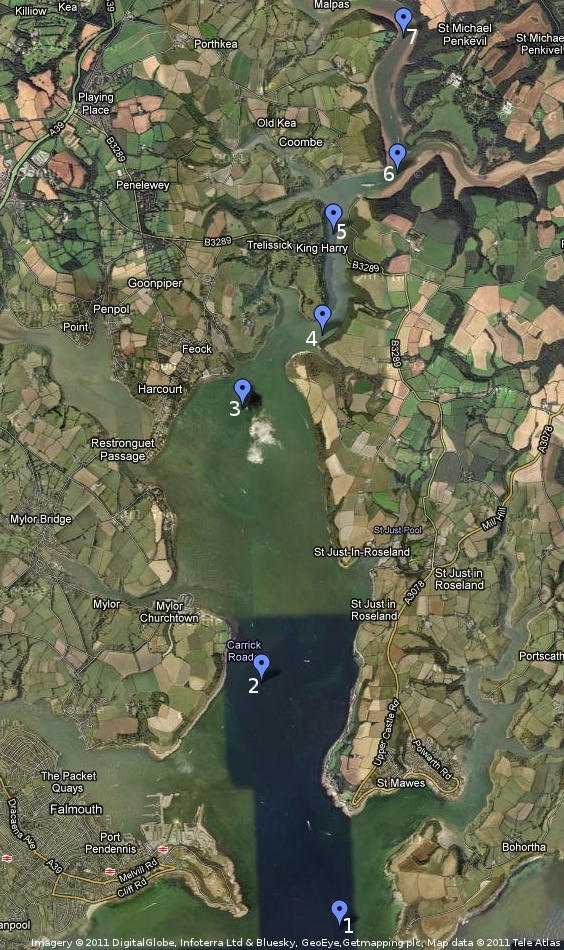
Figure 1: Map of CTD stations
In order to determine the depth of 1% irradiance at each station, a secchi disk was lowered over the side of the vessel. At the point at which sight of the disc was lost, the length of the line was recorded alongside the angle of the rope in relation to the water surface. Using these parameters, the depth of the disc was calculated and then multiplied by 3. This takes into account the distance to the secchi disc, back to the surface and the refraction. The same person deployed the secchi disk at each station to account for perceptive differences, in areas of similar light conditions. It was found at station one that the length of rope was too short, the end of the rope being reached with the secchi still in clear view. While time did not allow for a repeat measurement at this station, extra rope was attached to the secchi for subsequent stations to ensure enough rope was available.
Figure 2: How an ADCP works
An Acoustic Doppler Current Profiler (ADCP) mounted to the hull of the R.V. Bill Conway, was used to measure the velocity of the water column. An ADCP emits 'pings 'of sound of constant high frequency into the water column. It then measures the Doppler shift of sound waves reflected from suspended particles moving in the water column to calculate the speed and direction of motion of the water. Consequently, the time elapsed between the 'ping' and receiving the echo is used to calculate the distance/depth from ADCP to the particle/current (WHOI, 2011; Figure 2). The data was stored and displayed using an on-board computer running WinRiver II
Horizontal transects were taken to provide a cross-section of the water velocity within the channel at 6 locations as shown in Table 1 below.
| Line | Start | End | ||||
|---|---|---|---|---|---|---|
| Latitude (N) | Longitude (W) | Time (GMT) | Latitude (N) | Longitude (W) | Time (GMT) | |
| 1 | 50°08.612 | 005°02.491 | 08:46 | 50°08.462 | 005°01.084 | 09:02 |
| 2 | 50°10.144 | 005°02.714 | 09:44 | 50°10.169 | 005°01.411 | 09:59 |
| 3 | 50°12.139 | 005°02.679 | 10:49 | 50°12.085 | 005°02.078 | 10:55 |
| 4 | 50°12.373 | 005°01.804 | 11:16 | 50°12.502 | 005°01.869 | 11:19 |
| 5 | 50°13.087 | 005°01.639 | 11:56 | 50°13.079 | 005°01.526 | 11:58 |
| 6 | 50°13.472 | 005°00.953 | 12:17 | 50°13.520 | 005°01.040 | 12:20 |
5 dummy plots were also taken over the journey between sample sites to ensure that data recorded was in relation to the estuary as a whole- however this data was not analysed.
The salinity and temperature depth profiles (Figure 3 and 4) show that the estuary is a well mixed or partially mixed estuary throughout its length, as there is little variation of either salinity or temperature with depth. The Richardson Number calculation also supports this, with the highest flow speed, of 0.222ms-1 was found at the mouth of the estuary; with a low flow speed of 0.0012ms-1 at the riverine input area. Furthermore, there is very little surface salinity variation from the head of the estuary to the area of riverine input. The salinity varies from 35.32 at the mouth of the estuary, to 31.68 at the most riverine sample site. The small change in salinity yet again implies a well mixed estuary.
The CTD depth profiles incorporated a chlorophyll a fluorometer and a transmissometer (transmittance is an indicator of suspended sediment concentration). It was expected that the fluorometer values would increase as distance from riverine input decreases, due to more chlorophyll being present in less saline waters. The transmissometer values were expected to decrease towards the fresh water input, as there was more sediment present in the riverine water. The fluorometer values increased from 0.11v at station 1 to 0.34v at station 8. The transmittance changed from 4.45v at station 1 to 3.90v at station 8.
Note: Station 7 doesn't appear on the graphs, because the CTD wasn't given enough time to adjust and the measurements aren't reliable.
The Richardson's Number is used to give an idea of the amount of mixing taking place in the water column; it is essentially the ratio between stratification of the water column and the shear stress attempting to mix it.
If Ri < 0.25 then there is turbulence and the water column is said to be well mixed; if Ri ≥ 1 then flow is laminar and the water column will be stratified. Values between 0.25 and 1 are a grey area, but are is classified as partial mixing.
The Richardson's number was calculated at each ADCP transect using this data plus data retrieved from the CTD profiles.
| Station | CTD Profile | Richardson's Number |
|---|---|---|
| 1 | 1 | 0.010 |
| 2 | 2 | 0.005 |
| 3 | 3 | 0.002 |
| 4 | 4 | 0.003 |
| 5 | 5 | 0.003 |
| 6 | 6 | 0.004 |
| 7 | 8 | 0.001 |
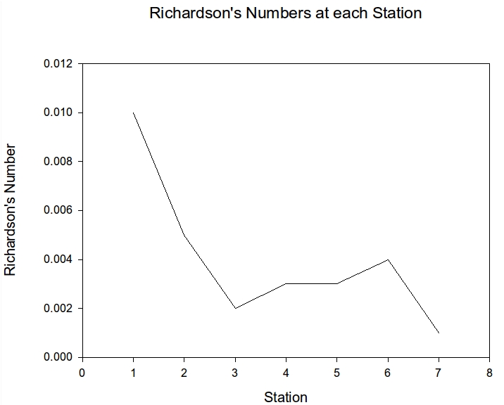
Figure 5: Richardson numbers for 7 stations in the Fal estuary
The results show that Ri is less than 0.25 throughout the estuary meaning there is turbulence and the water column will not be stratified; this is as expected as the Fal is said to be a well mixed or partially mixed estuary. There is also a general decrease in Ri as you move up the estuary; this will be due to the decrease in depth as there is much higher shear at the bed causing more turbulence in the water column.
The residence time of the estuary (flushing time) was calculated using the formula:
| Tres = | (1 - Smean/Ssea) x Vtotal |
| R |
| Tres: | Residence Time (s) |
| Smean: | Mean salinity |
| Ssea: | Sea Salinity |
| Vtotal: | Total volume of estuary (m3) |
| R: | Riverine flux (m3s-1) |
This formula rather than the tidal method was used due to having more data further north in the estuary, which was less tidally dominated. The volume of the estuary was calculated using the cross-sectional areas of the horizontal transects (calculated by WinRiver) which are shown in Table 4.
| Transect No. | Location of start of transect | Cross Sectional Area (m2) | |
|---|---|---|---|
| Latitude (N) | Longitude (W) | ||
| 1 | 50°08.612 | 005°02.491 | 20662.38 |
| 2 | 50°10.144 | 005°02.714 | 6481.70 |
| 3 | 50°12.139 | 005°02.679 | 4081.98 |
| 4 | 50°12.373 | 005°01.804 | 2644.95 |
| 5 | 50°13.087 | 005°01.639 | 1752.84 |
| 6 | 50°13.472 | 005°00.953 | 1297.09 |
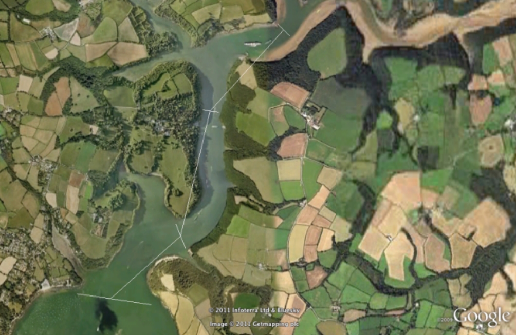
Figure 6: Marked are 3 transects used to calculate the residence time of the estuary
Transect numbers 1 and 2 did not have complete data therefore they were excluded from the calculation of the residence time, which instead only examined the upper estuary above Pill Pt. The volume of the upper estuary was found to be 7509124m3, calculated by finding the volumes of 3 truncated pyramids. This was done by treating the cross-sectional areas of transects 3-6 as 4 differently sized squares, measuring the distances between transects on Google Earth (Figure 6) and using these values in the equation 1⁄3(a2 + ab + b2). This is a rough approximation as it assumes that the estuary is straight and the channel depth increases at a steady rate.
The mean salinity of 33.85 calculated from CTD data at stations 1-8 and the Ssea of 34.89 was the surface salinity measured by the CTD at Station 3. The riverine flux/freshwater input value (R) was calculated from flow data taken from the Fal at Tregony (NERC). The average of data recorded in July between 1999 and 2009 was found to be 1.16ms-1. It should be noted that Tregony is a relatively long way up the river Fal and the Fal is not the only freshwater input (it was not possible to download data for the K station), therefore R is likely an underestimation.
| Tres = | (1 - 33.85/34.89) x 7509124 | = 193481s = 53.7 hours = 2.24 days |
| 1.16 |
To determine the dissolved phosphate and silicon content, samples were taken using Niskin bottles at specific depths at 7 stations to show varying water masses (Table 1). All samples were filtered onboard to remove phytoplankton and zooplankton. Each of the plastic (for Si) and glass (for P) bottles was rinsed with 10cm3 of the sample; another 40cm3 of the sample was dispensed into the bottle and stored at constant low temperature. The samples were then analysed on 4/07/2011 using the method presented by Parsons et al. (1984).
The water samples for oxygen concentration analysis were collected at stations 1-4 and station 7 at each depth (Table 1). Water was drawn directly from Niskin bottles prior to opening them via a nozzle at the bottom and was used to rinse the BOD bottles and then fill them with water to be sampled. With a pipette 1ml of manganous sulphate was added to each sample followed by 1ml of alkali-iodide-azide. The bottles were carefully closed to prevent air bubbles being trapped inside and each bottle was inverted several times to allow the reagents to mix and bind to dissolved oxygen. Flakes of precipitate started forming in the solution and the bottles were inverted again after the precipitate settled to about half the volume of the bottle. The sample bottles were put into a bucket filled with seawater to prevent desiccation of the lid and contamination of the sample. The samples were analysed on 4/07/2011 using the method described by Grasshoff et al. (1999).
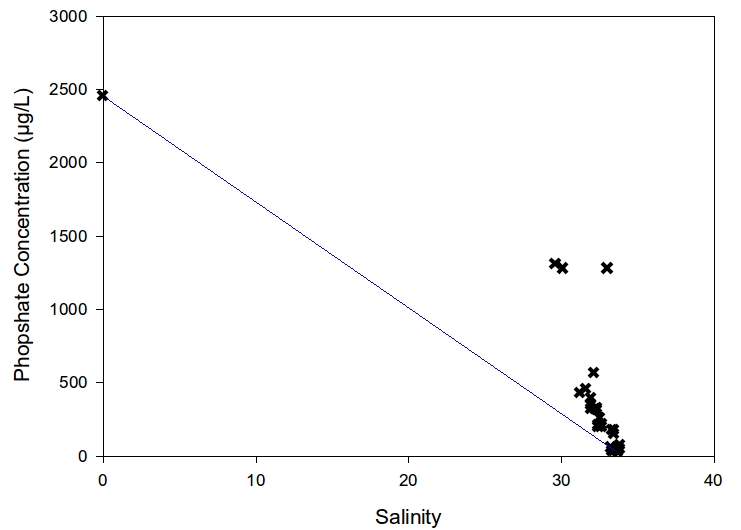
Firstly, analysis of Phosphate samples showed a decreasing trend with increasing salinity and therefore distance downstream in the Fal estuary. This is illustrated in Figure 7 which is an estuarine mixing diagram, with the blue line being the TDL (theoretical dilution line). The majority of the data points lay above the TDL. The maximum phosphate concentration was 2457.7μg.L-1 at 0 salinity (riverine end member) and the minimum sampled concentration was 29μg.L-1 at 50°10.130 N, 5°02.348 W at the second station sampled, with a depth of 3.11m.
 |
 |
|---|---|
Figure 7: Estuarine mixing diagram plotting phosphorous concentration against salinity | Figure 8: Estuarine mixing diagram plotting silicon concentration against salinity |
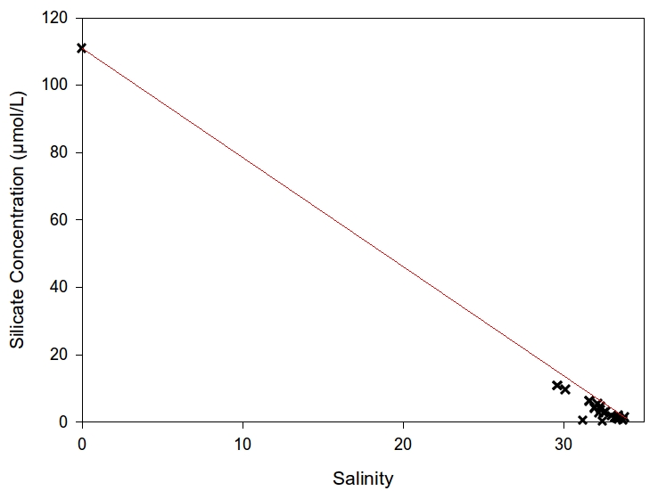
Once the blank corrections were made, an estuarine mixing diagram, with red TDL was produced of the dissolved silicon (DSi) concentrations (Figure 8). Again similar to the Phosphate there is a decreasing trend in DSi with increasing salinity and distance. The maximum DSi concentration was 110.9471μmol.L-1 which was measured at zero salinity (i.e. river end member). The minimum recorded DSi was 0.471μmol.L-1 at a salinity value of 33.7 which was taken from 50°08.519 N, 005°01.516 W with a depth of 9.17m.
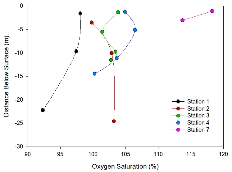
Dissolved oxygen is plotted against depth in Figure 9 and shows a decrease in oxygen saturation with depth below the surface in general. At station 4 it slightly increases from 104% to 106% at the surface, at station 3 between 5 and 10m depth and overall it increases in station 2. The maximum oxygen saturation is 118% at 50°14.394 N, 5°00.885W at station 7, near the top of the estuary where the depth of the sample was 14cm (sub-surface). The most depleated area was 50°08.538 N, 5°01.466 W at a depth of 21.33m at the mouth of the estuary where the oxygen saturation was 92.3%.
 |
|---|
Figure 9: Plot of dissolved oxygen concentration against depth for 7 stations in the Fal estuary |
The phosphate data shows input into the system other than the original influx from the Fal river, as the majority of the data points lay above the TDL. It is highly probable that sewage output from sewage works at 50°14.900 N, 5°02.600 W (Truro river) and 50016.540 N, 5°0.460 W (Tresillian river) is high in phosphates. The MBA who assigned special area status to this area have shown that 26-62% of phosphate influx is from sewage treatment centres (Langston et al., 2003). Non-biological removal by coagulation due to mixing (Morris et al., 1980) is also possible.
DSi levels in estuaries generally follow a trend where the DSi decreases with increasing salinity (Chou & Wollast, 2006), it can be suggested that the Fal Estuary follows this trend. Given that estuaries are usually characterised by high biological activity, including diatoms, caused by the large input of nutrients derived from land (Tréguer et al., 1995). Thus, it can be suggested that this biological activity is the reason that removal is occurring in the Fal. This is because diatoms need DSi, which is present in both cell contents and the frustules (Ittekkot et al., 2006) and therefore is essential for their growth. This would mean that as the DSi travels down the estuary the diatoms present will begin to consume the DSi and therefore will give a non-conservative line on the TDL.
The oxygen saturation is highest in surface waters of stations 1 and 7 possibly due to blooms of phytoplankton producing oxygen as a bi-product of photosynthesis, and then decreases with depth due to grazing from zooplankton, respiration of bacteria and decrease in irradiance leading to less photosynthesis. Lower salinities at the surface from freshwater run offs and cooler surface temperatures may also have led to higher oxygen saturation aiding in dissolution of oxygen. It is possible that stations 3 and 4 shows some deeper oxygen production maybe by photosynthesising dinoflagellates and but at station 3 utilisation of oxygen may be higher than production. Finally station 2 may have an oxygen depleted surface water due to grazing at the surface, or due to respiration being greater than photosynthesis (Miller, 2003).
Plankton samples were taken at station 1, 3 and 7, each representing lower, mid and upper estuary respectively. A plankton net was towed at constant speed and depth behind the boat to collect each sample. The net had an inlet diameter of 52cm, and a mesh size of 210μm. Once each station was sampled, the net was rinsed with a hose supplied with water by an impeller pump from the immediate surrounding water. The rinse washed the sample into an attached 1 litre bottle, to which 50ml of formalin was added to preserve the sample. In order to account for variable rate of flow between stations, and subsequent variability in plankton counts, the revolutions of a small rotor, suspended in the centre of the net inlet were recorded both before and after the net was deployed, the difference between which was used in conjunction with plankton counts to determine plankton density at each station.
Chlorophyll samples were collected at stations 1-7 with 2 replicates at each depth (Table 1). 50cm3 of seawater was filtered through 64μm filter and these were stored in plastic test tubes containing 6cm3 of 90% acetone solution. The samples were stored in a refridgerator to prevent degradation and chlorophyll a concentration was determined on 4/07/2011 using AU-10 fluorometer. The average was calculated for replicates that had similar readings and the highest concentration value was taken if the readings had more that 10% difference.
Surface phytoplankton samples were collected at stations 1-5 and station 7 from Niskin bottles containing water collected closest to the surface (Table 1). 100ml of water were added to a glass bottle containing 10ml lugols iodine solution and the bottles were stored until the the samples were analysed on 4/07/2011. Phytoplankton cell number per litre was estimated by counting individual cells under the microscope. The dominant phytoplankton taxa were identified as well.
Chlorophyll concentrations in the surface waters at each station were used along with the phytoplankton cell concentration per litre to plot the values and allow for their comparison (Figure 10). Proportion of each group of phytoplankton was calculated relative to the total number of cells per litre for each station to be able to analyse how the distribution of different phytoplankton taxa varies along the estuary (Figure 10). The dominant taxa were identified and are provided in Table 5.
| Station | Dinoflagellates | Diatoms | Euglenoids |
|---|---|---|---|
| 1 & 2 | Alexandrium minutum | Thalassiosira spp. (Thalassiosira rotula) Cheatoceros spp. Rhizosolenia spp. (Proboscia alata) | Eureptiella spp. |
| 3 | - | Proboscia alata (4.4%) Thalassiosira spp. (75.3%) Chaetoceros spp. (20.3%) | |
| 4 | - | - | |
| 5 | Alexandrium minutum | Rhizosolenia spp. (Rhizosolenia stiliformis) Thalassiosira spp. (Thalassiosira rotula) Cerataulina spp. (Cerataulina pelagica) | |
| 7 | Alexandrium spp. | Thalassiosira spp. (95.3%) Cylindrotheca closterium (4.6%) |
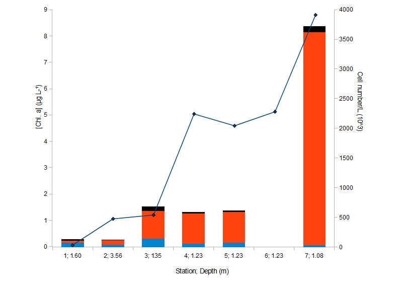
Figure 10: Major phytoplankton taxa and chlorophyll concentrations at 7 CTD stations
Chlorophyll a concentrations are often used as an estimate for the phytoplankton biomass, however, one must take into account that Chl. a is not the only pigment present in phytoplankton. Other major pigments present in dinoflagellates include peridinin, diadinoxanthin, carotene as well as other types of chlorophyll, combined, their concentration often exceeds chl. a concentration. Diatoms, on the other hand, might have fucoxanthin concentrations almost equal to those of chl. a,(Schluter et al., 2000). Indeed, the data from Figure 10 shows that between stations 1 and 2 the chlorophyll concentrations increased, while the cell concentration stayed almost the same. Between stations 2 and 3 there was only slight increase in chl. a concentration while the cell number/L increased almost sixfold. Also, a significant increase in chl. a concentration opposed to a decrease in cell number/L can be observed between stations 3 and 4. These observations confirm that Chl. a concentrations alone do not provide an accurate account of phytoplankton biomass and it is crucial to have some other measure of phytoplankton concentrations, which, in the case of the survey, was estimating the number of cells/L.
Figure 10 provides a picture of phytoplankton taxa distribution along the estuary and it can be observed that the proportion of dinoflagellates decreased from the mouth of the estuary up the river, while diatoms showed an opposite trend. Euglenoids only seemed to make up a significant proportion of the total phytoplankton at stations 1 and 3 and were not very abundant compared to the two other groups at the rest of the stations.
Grazing pressure was likely to affect the biomass of phytoplankton in the mouth of the estuary as well as increase dinoflagellate to diatom ratio. In the upper estuary the grazing pressure was significantly lower and the availability of silicate and turbid waters, unfavourable for dinoflagellates, positively affected the diatom species, allowing the biomass to increase significantly compared to other parts of the estuary. The species composition of diatoms also varied at different stations as can be seen from Table 5. Diatoms showed the the highest variation, for example, at station 3 the dominant group were Thalassiosira spp. (75.3%), followed by Chaetoceros spp. (20.3%) and Proboscia alata (4.4%). At station 7 Thalassiosira spp. still dominated but Proboscia alata was absent, and Chaetoceros spp. very rare; instead, Cylindrotheca closterium formed 4.6% of all the phytoplankton present.
Clear patterns of the abundance and composition of zooplankton sampled at each station are observed, the most distinct of which is a decreasing number of species and total abundance as you move up the estuary.
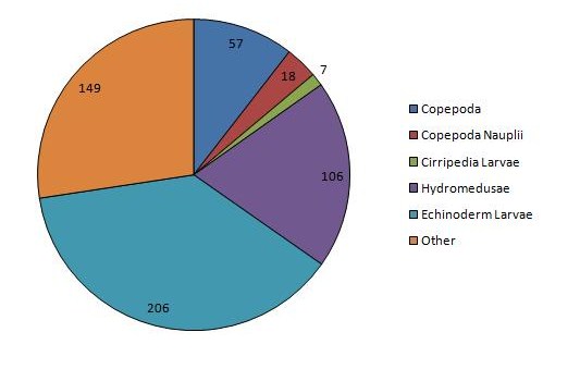
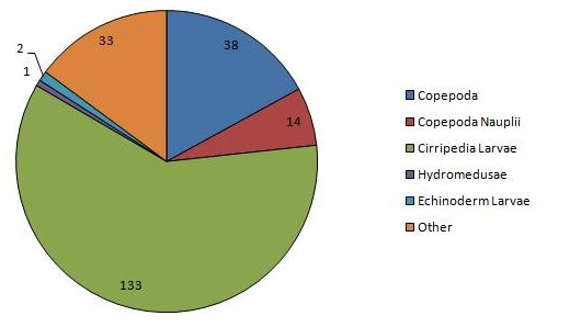
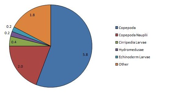
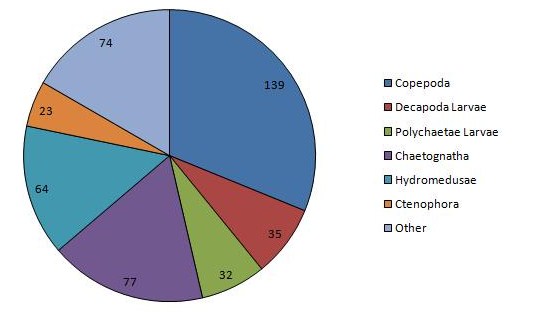
The sample in the lower estuary, CTD1, was dominated by echinoderm larvae, hydromedusae, copepods and siphonophores at densities of 206, 106, 57, and 41 individuals m-3 respectively. This station was also the only station at which any individuals were identified as fish larvae, nemertea, tunicata, ctenophora or mysidacea. CTD1 also had the highest zooplankton abundance of the stations, with a total count of 554 individuals. Very high dominance of larval cirripedes is observed mid estuary, at CTD3, with a calculated density of 133 individuals m-3, while copepoda have the next greatest density of just 38 individuals m-3. Echinoderm larvae are still present, although at a much lower density of 2 individuals m-3, while no tunicata, nemertea, ctenophora or fish larvae was identified. The presence of cladocera was observed at CTD 3, and is the only station where they occur. The abundance of zooplankton sharply decreases at this station, with a total count of 222 individuals, less than half that observed at CTD 1. Sampling at CTD7 sees the loss of further groups siphonophorae, gastropoda and cladocera, with copepods as the dominant group at a density of 6 individuals m-3 and copepod nauplii at a density of 2 individuals m-3, the only groups present at a density of more than 1 individual m-3. CTD7 has the lowest total count of the sample sites, of just 10 individuals m-3
 |
 |
 |
|---|---|---|
Figure 11: Chart of the dominant zooplankton at CTD station 1 | Figure 12: Chart of the dominant zooplankton at CTD station 3 | Figure 13: Chart of the dominant zooplankton at CTD station 7 |
The research carried out in the Fal Estuary confirmed that it was a well mixed estuary and demonstrated a sensitive relationship between the physical, chemical and biological factors affecting the estuarine environment.
Station 1 at the mouth of the river showed the greatest flow rate and the lowest turbulence. Consequently, there was less oxygen circulated to depth. Low phytoplankton concentrations as opposed to high amount of zooplankton, suggested that grazing had increased after a spring bloom. As grazers generally prefer diatoms to dinoflagellates, the latter gained from lower grazing pressure and formed a higher proportion of the total phytoplankton biomass. This correlates to the distribution of the nutrients, as silicon appears to be replenishing with little removal by diatoms. The low diatom abundance here would have been compounded by the high grazing pressure of abundant zooplankton, preferentially selecting diatoms over dinoflagellates, as recorded by Porter (1973).
With progression up the estuary, phytoplankton biomass increased until it reached a plateau. This increase may have been accelerated due to the amplified PO4 concentration from sewage waste outfall. Further upstream from the outfall the phytoplankton biomass recovered to its previous rate. However this could be a result of natural input of nutrients flowing downstream and decrease in grazing pressure. In contrast with the increasing abundance of phytoplankton, both the abundance and species richness of zooplankton decreased mid estuary, with an abundance of less than half of that observed at station 1, although with massively increase abundance of larval cirripedia. Alternatively another interpretation, is that the plankton reached a plateau and stopped increasing because of the low flow and turbulence rates resulting in weak mixing within the estuary. Therefore it was trapped in deeper layers and did not have enough access to light.
At the top of the river the flow rate was the slowest and turbulence was highest. The lowest salinity and the maximum phytoplankton biomass lead to the highest percentage of oxygen saturation. The composition of the phytoplankton consisted of mainly diatoms as unfavorable conditions reduced the number of dinoflagellates. Zooplankton was found at the lowest densities here, coinciding with the lowest observed species richness.
The high zooplankton abundance at the mouth of the estuary may be a compounded effect of both the preferential conditions found there, and by the 'flushing' of zooplankton out of the estuary by the ebbing tide (Barlow, 1995). Both hydromedusae and echinoderm larvae require high, stable salinities to survive, and reproduce in the summer months (Christian et al 2010), explaining the high densities recorded at station1, and also their subsequent absence from stations further up the estuary. It has been shown that zooplankton will preferentially seek out areas of low flow velocity to try and maintain their desired position within the estuary (Wooldridge et al, 1980) . As these flows are often subsurface, our sampling method would not have collected these, our sample consisting just of individuals lost from the population due to the tides (Wooldridge et al, 1980). The persistence of copepods throughout the estuary, albeit at varying densities, is likely due to the variation in resistance to salinity stress and swimming strength between their species (Wooldridge et al, 1980; Barlow, 1995). The very high densities of larval cirripedia mid estuary is likely due to localized spawning of nearby barnacles, while their absence at the estuary mouth is explained by the retention the larval form by the cirripedia only within estuaries, developing into adults when marine conditions are met (Macho et al, 2010).
The ACDP could only record reliable data between depths of ~3m and ~20m. Quantifying phytoplankton cells and their identification under the microscope was subjective, resulting from the lack of experience in taxonomy and was most likely an underestimation of the actual phytoplankton concentrations.
The aim of the fieldwork was to collect the data to compare the chemical, physical and biological properties of the offshore water column to those of the estuarine environment. This will help establish how vertical mixing processes affect the structure of plankton communities.
A survey was carried out on 06/07/2011, from 08:14 to 13:05 (GMT) on the R.V. Callista, a twin hull purpose built research vessel just under 20 meters long. A large aft deck with an A frame allows for large equipment deployment. It was an overcast and rainy day, with cloud cover starting at 4⁄8 and progressing to 8⁄8 over the course of the survey. The met office forecast for the practical was:
| Wind: | Southwest 5 to 7, occasionally gale 8 at first, decreasing 4 or 5 later. |
|---|---|
| Sea State: | Very rough at first in west, otherwise moderate or rough. |
| Weather: | Rain or squally showers. |
| Visibility: | Moderate or good. |
The weather conditions limited the extent and timespan of the survey, therefore, the initial plan to work offshore had to be modified and the boat work was carried out in the coastal area of the Falmouth Bay. Table "Locations of sampled stations and depths sampled" below shows the locations the vertical samples were conducted , the depths sampled and the time taken at each location. Table "Locations of transects conducted with the ADCP and their durations" shows the transects sampled using the ADCP (Acoustic Doppler Current Profiler).
| Station | Location (WGS'84) | Depth (m) | Start Time (GMT) | |||
|---|---|---|---|---|---|---|
| Latitude (N) | Longitude (W) | |||||
| 1 | 50°08.646 | 005°01.430 | 16.0 | 1.3 | 08:14 | |
| 2 | 50°04.345 | 005°03.246 | 26.0 | 12.0 | 1.0 | 09:46 |
| 3 | 50°05.453 | 005°04.293 | 13.0 | 1.5 | 10:51 | |
| 4 | 50°08.765 | 005°01.649 | 1.6 | 13:01 | ||
| Number | Start | End | ||||
|---|---|---|---|---|---|---|
| Latitude | Longitude | Time | Latitude | Longitude | Time@ | |
| 1 | 50°08.610 | 005°01.470 | 08:02 | 50°08.639 | 005°01.339 | 08:55 |
| 2 | 50°08.639 | 005°01.339 | 08:55 | 50°04.354 | 005°03.282 | 09:39 |
| 3 | 50°04.384 | 005°03.282 | 09:39 | 50°04.286 | 005°03.017 | 10:30 |
| 4 | 50°04.286 | 005°03.017 | 10:30 | 50°05.386 | 005°04.282 | 10:45 |
| 5 | 50°05.386 | 005°04.282 | 10:45 | 50°05.545 | 005°03.825 | 11:19 |
| 6* | 50°05.545 | 005°03.825 | 11:19 | 50°05.402 | 005°03.786 | 11:21 |
| 7 | 50°05.297 | 005°04.295 | 11:28 | 50°06.065 | 005°05.270 | 11:41 |
| 8 | 50°06.065 | 005°05.270 | 11:41 | 50°06.050 | 005°05.239 | 11:43 |
| 9 | 50°06.050 | 005°05.239 | 11:43 | 50°05.346 | 005°04.386 | 12:00 |
| 10 | 50°05.499 | 005°04.140 | 12:03 | 50°09.119 | 005°01.645 | 12:55 |
In terms of physical data collection a range of equipment were used, including a secchi disk, ADCP, a TS probe and a CTD. The CTD provided measurements of temperature and salinity variations with depth. It also had a fluorometer and transmissometer attached which measured turbidity and chlorophyll fluorescence. Measurements were taken at the pre-determined stations (Table 1) and the rosette itself required lifting and lowering into the water column with guidance ropes attached to the A frame of the vessel. A TS probe was used to measure temperature and salinity changes in a water supply pumped on board from the surface by a peristaltic pump. This method was also used to gain surface water samples at station 4 as the conditions did not allow for equipment to be deployed. In order to determine the depth of 1% irradiance at each station, a secchi disk was lowered over the side of the vessel at each station by the same person to reduce any human error or difference in judgement. The ADCP was used to determine the speed of the water flow, its direction and other physical parameters, which can be measured using Doppler shift techniques.
Station 1
Flow velocity decreases with depth. Surface values vary between 0.1ms-1 and 0.6ms-1. Below 12m velocity values are typically less than 0.13ms-1. Flow at the surface is in the North-East direction, flow at depth (below 12m) is in the Northerly direction. There is quite a large amount of variability in the flow direction. Location just out of the river mouth therefore should have a layer of fresh water, however it was high water and the Fal is a well mixed estuary.
Station 2
Water in surface 10m is flowing in an Easterly/South-Easterly direction. Water below 10m is flowing in a southerly/south-westerly direction. Velocity is fairly constant through the water column, varying between 0.04ms-1 and 0.4ms-1.
Station 3
Water was flowing in a southerly direction below 10m. Water in upper 10m was flowing in an Easterly/South-Easterly direction. Flow velocity is fairly uniform through the water column, varying between 0.05ms-1 and 0.25ms-1, with water in the top 10m flowing slightly faster than the water below it.
It was not possible to get any relevant information from the backscatter data at the stations due to the movement of the boat and the bad weather.
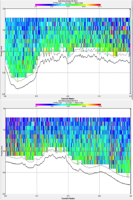
Figure 1: Velocity magnitude measured using an ADCP across a horzontal transect of the Fal estuary
Figure 1 appears to show a faster water mass flowing in an East/South-Easterly direction over another with a boundary at approximately 7m, water mass flowing in a South/South-Westerly direction. This is confirmed by the Ship Track Plots. The velocities of the flow decreased between the first and second transect due to the tidal state.
Highest velocities recorded are in the top 5m of the channel (deepest part of the transect) flowing in a South Easterly direction. Typical values here are between 0.2 and 0.45ms-1. The majority of the rest of the water appears to have a velocity of approximately 0.2ms-1, varying between 0.6ms-1 and 0.4ms-1.
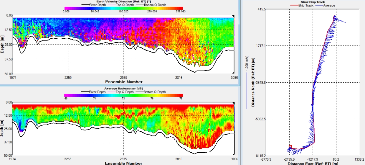
Figure 2: Velocity direction, backscatter and ship track measured using an ADCP across a horizontal transect of the Fal estuary
Figure 2 shows the journey between station 1 and 2. As HW was at 08.40 GMT (Height: 5m) and the boat travelled from Station 1 to Station 2 between 08.55 and 09.39 (GMT), this transect shows how flow along the coastline changes temporally depending on tidal state. This can be seen on the Stick Ship Track Plot and the Velocity Direction Contour plot. Due to the rough weather, the top 5m of data on the backscatter graph can be ignored. Patches of zooplankton can be seen in red in the middle of the water column, waves can also be seen in these patches. A turbidity maximum above the seabed can also be seen in red towards the end of the transect, due to the change of the tide. Crossed the Helford outflow, however the transect was a large distance from the shore, so it was likely that the changes seen are temporal rather than due to different water masses.
Three CTD depth profiles were carried out during the offshore investigation and can be seen on Figure 3, along with the ADCP transects. The weather restricted the area into which we could sample, creating a small physical data set with very little variation. The data collected from the CTD was used in conjunction with the chemical analysis to produce depth profiles for varying constituents at the three sample sites.
A blank transmissometer reading was taken, to allow the recorded values to be changed into absolute values. The blank reading was 0.06v, so the transmissometer values had 0.06v taken away before being implemented onto the graphs. However the transmissometer values were not put onto graphs because they didn't show variation with depth.

Figure 3: Map of offshore ADCP transects and CTD stations taken around the Falmouth coast
The Richardson's Number's meaning and use, including its equation, is shown in the estuarine analysis above. For this offshore analysis, the Richardson's number (Ri) was calculated at set depths for each of the three CTD stations; this helps to show if there are any stratified areas in the water column.
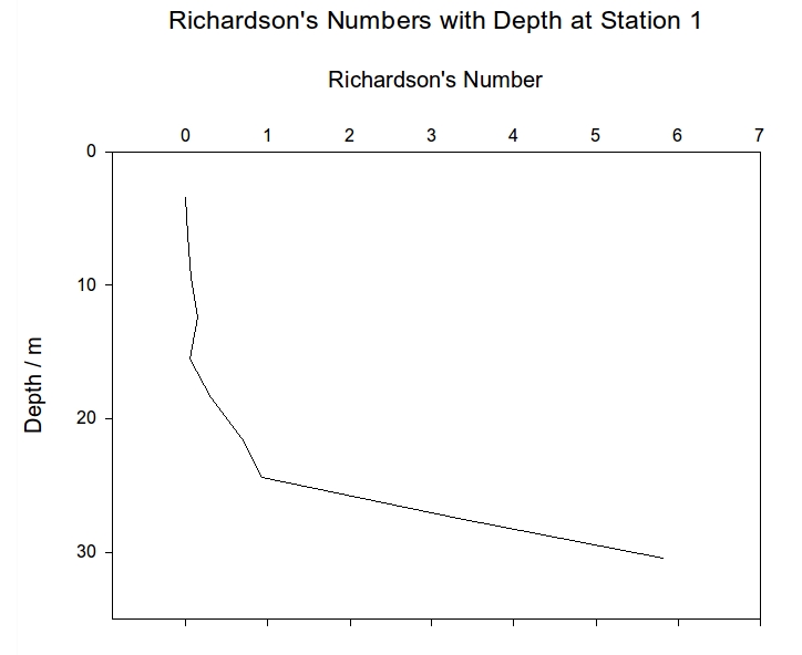
All of the stations show an increase in Ri as you move down the water column showing that there is more stability at higher depths. At station 1, Ri remains below 0.25 until about 18m where there is a sudden increase to almost 6 at 30m. This shows that the water column is well mixed and turbulent above 18m but laminar and stable below this depth.
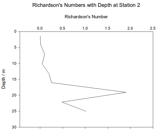
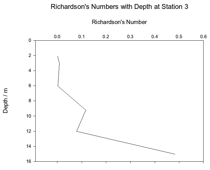
Station 2 shows the same general increase in Ri with depth but also shows a sharp spike at 19m; this could be showing a layer of stable laminar water between two well mixed layers. Station 3 has Ri of below 0.25 for the entire water column until the final depth of 15m which has a Ri of 0.48, this value is still not above 1 which is when the water is considered to be stratified therefore the entire water column of station 3 is well mixed with no stratification. The Ri values for the entire water column at each station show station 2 to the only stable environment with a value of 1.33 whereas stations 1 and 3 both show signs of partial mixing with values of 0.62 and 0.43.
 |
 |
 |
|---|---|---|
Figure 4: Richardson numbers plotted against depth for CTD station 1 | Figure 5: Richardson numbers plotted against depth for CTD station 2 | Figure 6: Richardson numbers plotted against depth for CTD station 3 |
Niskin bottles were used to take water samples at depth, and these were also operated using a winch system, from which individual bottles were positioned at depth, closed by a messenger object and hauled to the surface. Silicate and phosphate samples were prepared on board from the collected water by filtration into plastic and brown glass bottles respectively. Each of the bottles was rinsed with 10cm3 of the sample; another 40 cm3 of the sample were filtered into the bottle and stored at a constant low temperature.
The water samples for oxygen concentration analysis were collected at stations 1-3 at each depth (Table: Locations of sampled stations and depths sampled.) Water was drawn directly from Niskin bottles prior to opening them via a nozzle at the bottom and was used to rinse the BOD bottles and then fill them with water to be sampled. Oxygen was fixed using the same method as described in the Estuarine section of this website.
The analysis of the water samples took place on 07/07/2011 and the laboratory techniques were identical to those explained in the Estuarine section of this website.
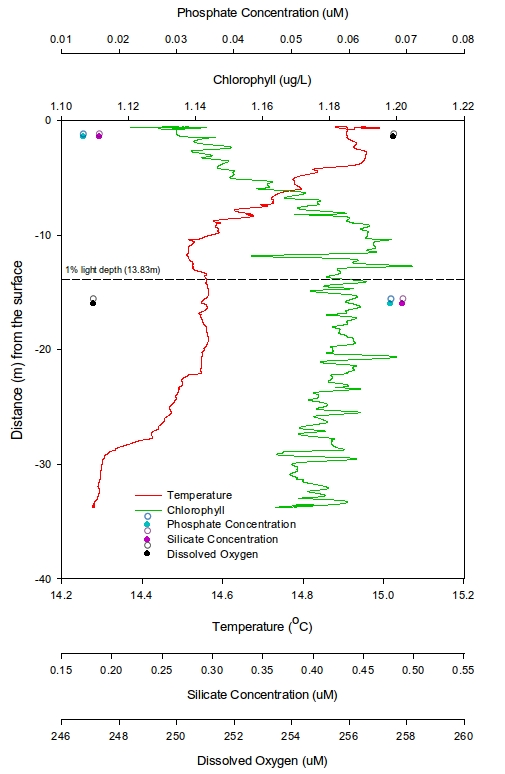
At station 1 (Figure 7), the first trend seen is that temperature decreases from 15°C rapidly down to a depth of around 11m. A plateau appears from over the next 10m from which point it slowly reduces to a minimum of 14.3°C. The chlorophyll shows a lowest value of 1.12μgL-1 at 0.6m depth, increasing to 1.19μgL-1 at 10.5m and then becomes constant with depth. Given that only two depth points for both dissolved silicon (DSi) and Phosphate were sampled, it is not viable to suggest any general trends but instead just state the values that were recorded. DSi had a highest value of 0.49μmol L-1 at 16m and a lowest concentration of 0.19 μmol L-1 at 1.5m. Similarly with Phosphate the highest value of 0.067 μmol L-1 was at 16m and the lowest concentration of 0.014 μmol L-1 at 1.5m. In contrast the highest dissolved oxygen value occurs at 1.5m (257.6μM) and lowest value at 16m (247.1μM). The 1% light depth was recorded at 13.83m.
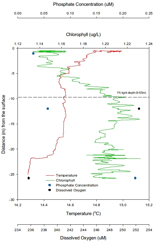
At station 2 (Figure 8), the same trend in temperature seen in Station 1 is seen but the plateau is shallow (from 5m-17m). Chlorophyll exhibited the same trend seen in section 1 where it showed the lowest value at 0.8m (1.13μgL-1) and a high value of 1.22μgL-1 at 11.2m. One note to make in the nutrients is that DSi had a value of 0 at this station so was not plotted. 3 Phosphate values were collected at this station, highest at 26m (0.22μM) and lowest at 1m (0.029μM). Dissolved oxygen showed a highest value at 12m (252.5μM) and a lowest value at 26m (235.6μM). The 1% light depth was slightly shallower than in station 1 (9.65%)
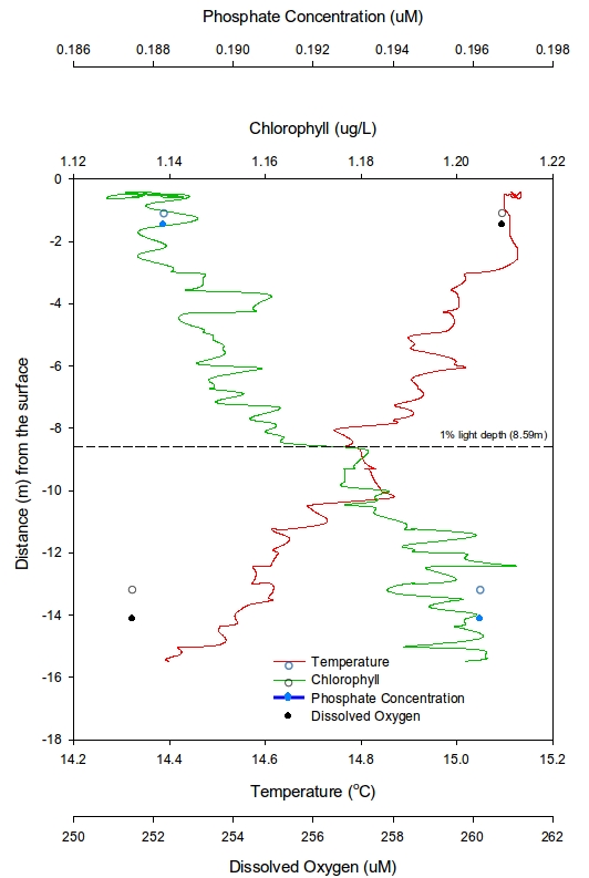
At station 3 (Figure 9) had a maximum sample depth of 14m and also showed no plateau in temperature. There was an overall linear decrease in chlorophyll from 1.13μgL-1 at 0.6m increasing to a high of 1.20μgL-1 at 15m. Again DSi recorded a value of 0, but phosphate showed values of 0.189μM at its shallowest depth (1.5m) and highest value of 0.1896μM at its lowest depth (14m). Dissolved oxygen showed a highest value at 1.5m (260.7μM) and a lowest value at 14m (251.0μM). The 1% light depth at this station showed the lowest value at 8.59m.
 |
 |
 |
|---|---|---|
Figure 7: Vertical profile from the CTD for chlorophyll, phosphate, temperature and dissolved oxygen for station 1 | Figure 8: Vertical profile from the CTD for chlorophyll, phosphate, temperature and dissolved oxygen for station 2 | Figure 9: Vertical profile from the CTD for chlorophyll, phosphate, temperature and dissolved oxygen for station 3 |
A slight thermocline is seen between 3 and 10m at station 1 (Black Rock) suggesting there was some form of stratification at this station. This was therefore likely to prevent mixing of nutrients between the overlying and underlying water masses. This suggestion is mirrored by the low phosphate and silicate (DSi) concentrations above the thermocline, where there was likely utilisation of these nutrients by phytoplankton previously, but little replenishment of stock due to lack of mixing.
The chlorophyll values indicate an increase in phytoplankton (chloroplasts) with depth and stability below the thermocline, which maybe suggests that the surface blooms of phytoplankton are suffering from lack of nutrient following exploitation of surface nutrients and no replenishment but this needs to be backed up by the biological data collected. Dissolved oxygen is lower below the 1% light depth which is likely to be caused by sufficiently less production due to lower irradiance.
Station 2 showed generally the same pattern as the first station. This sample was taken further from the mouth of the Fal estuary and therefore nutrient concentrations were much lower due to dissipation after release from the estuary, and this can be seen between stations 1 and 2. Silicate levels were so low due to usage and dissipation that they are not plotted on this graph. There is a thermocline here but this is at a much shallower depth, possibly due to more influence by the weather and disturbance at this point slightly further offshore than that of station 1.
The 1% light depth here is shallower, therefore the water is likely to have a greater turbidity here than at station 1. The phosphate concentrations seem to show an exponential decrease with depth, and this may be due to biological utilisation again above the thermocline which has led to depletion. Lack of mixing then allows this curve to form with greatest rate of use at the surface, decreasing with depth.
Station 3 was a shallower profile and therefore a decrease in temperature is seen linearly here although on a larger scale this may be seen as a steep gradient within the water column. This was offshore from the mouth of the Helford estuary. Chlorophyll values also decrease as at the other stations at a similar rate also. Phosphate concentrations and dissolved oxygen levels also show the same pattern as at other stations although both have greater surface concentrations here than at previous stations. This is possibly due to the shallow nature of the survey, the release from the Helford estuary, and/or the roughness of the sea at this point increasing mixing and changing circulation (Gemmrich et al., 1999) as weather conditions deteriorated further, allowing for upwelling of these parameters.
Zooplankton net that had a diameter of 62cm and a filter mesh size of 210μm was deployed at each station using a winch system over the A frame. This particular net also had a function of closing off the collection cup at a particular depth, which could aid the ability to observe vertical zooplankton distribution in the water column. Formalin was then added to the collected samples in order to preserve the zooplankton captured for further analysis.
Chlorophyll samples were produced at each station, with 2 replicates at each depth (Table: Locations of sampled stations and depths sampled). 50cm3 of seawater was filtered through 64μm filter and these were stored in plastic test tubes containing 6cm3 of 90% acetone solution. The samples were stored in a refrigerator to prevent degradation and analysed the following day in a laboratory.
Phytoplankton samples were collected at each depth from Niskin bottles. 100ml of collected water were added to a glass bottle containing 10ml lugols iodine solution and the bottles were stored until the samples were analysed on 07/07/2011. Phytoplankton cell number per litre was estimated by counting individual cells under the microscope. The dominant phytoplankton taxa were identified as well.
Chlorophyll concentrations at each depth at each station were plotted along with the phytoplankton cell concentration per litre to allow for their comparison. Proportion of each group of phytoplankton relative to the total number of cells per litre for each station was plotted as well (Figure 10). The dominant taxa were identified and are provided in TABLE "offshore taxa" HERE. Note: station 4 is placed together with station 1 as the locations were very similar.
Overall, chlorophyll a concentrations were very low and did not vary significantly with depth, ranging from 1.0 to 2.5 μg/L. The output data from the CTD fluorometer showed a weak peak in chlorophyll at around 13-10m depth at station 2, compared to the values from below the thermocline and near the surface (Figure 8) The samples, however, showed a different picture: the chlorophyll concentration was highest at 26m, but the cell number was the lowest and increased towards the surface (Figure 10). Station 2 samples from 26m and 12m were almost entirely dominated by diatom species, while at the rest of the stations and depths the proportion of dinoflagellates remained in the range of 19-32%. Again it was difficult to conclude whether chlorophyll a was a good measure of biomass, as samples with similar concentrations at the mouth of the Fal estuary (see Estuarine part) had several times more cells per litre than those from the coastal stations.
The dominant diatoms at all stations were Rhizosolenia spp., especially Proboscia alata, as well as Chaetoceros spp. Thalassiosira and Pseudo-nitzschia spp. were also present but in significantly lower numbers than the other two groups. The main dinoflagellate species seemed to be Alexandrium minutum, and on several occasions Protoperidinium divergens were noticed. The "other" group in Figure 10 refers mainly to euglenoid species.
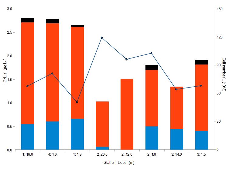
Figure 10: Major phytoplankton taxa and chlorophyll concentrations at 8 CTD stations
| Station | Depth (m) | Dinoflagellates | Diatoms |
|---|---|---|---|
| 1 | 16.0 | Alexandrium minutum Protoperidinium divergens Ceratium spp. | Chaetoceros spp. Rhizosolenia spp. (Proboscia alata, Rhizosolenia setigera) Guirnardia striata |
| 1.3 | Chaetoceros spp. Rhizosolenia spp.(Proboscia alata) | ||
| 4 | 1.6 | Alexandrium minutum | Chaetoceros spp. Rhizosolenia spp. |
| 2 | 26.0 | - | Rhizosolenia spp. Thalassiosira spp. Chaetoceros spp. Pseudo-nitzschia spp. |
| 12.0 | - | Chaetoceros spp. Rhizosolenia spp. | |
| 1.0 | Alexandrium minutum | Chaetoceros spp. Rhizosolenia spp. (Proboscia alata) | |
| 3 | 14.0 | Protoperidinium divergens | Rhizosolenia spp. Thalassiosira spp. (Thalassiosira rotula) |
| 1.5 | Alexandrium minutum | Rhizosolenia spp. (Proboscia alata) Thalassiosira spp. (Thalassiosira rotula) Pseudo-nitzschia spp. Leptocylindrus spp. |
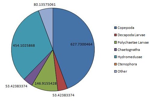
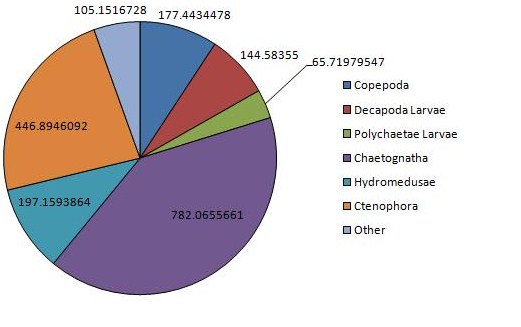
The vertical zonation of zooplankton is shown in (Figure 12, Figure 13), the deeper sample taken from 25.7m to 19.5m, is dominated by copepods and hydromedusae, but with chaetognaths present only at low densities. High dominance is observed here, rare species being completely absent, coinciding with a much greater total density of 1483m-3. The shallower sample taken from 12.6m to the surface shows a massively increased density of chaetognaths when compared with the water below but massively decreased copepods and hydromedusae. This is also the only station were ctenophores were observed in any significant densities. Rare species are present in similar densities at both depths, while decapod larvae are present in greater numbers at the surface, while larval polychaetes are more abundant at depth. Total density also increases at this greater depth, zooplankton present at densities of 1945m-3.
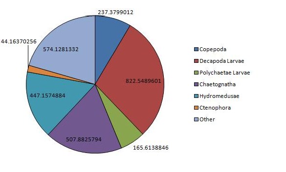
The greatest density of any one sample was observed at station 3, measuring 2826 animals m-3. Station 3 shows massive dominance of decapod larvae, which have otherwise been relatively absent from previous stations. Dramatically lower copepod densities are also observed here, especially when compared with the other surface samples, bottle 1 and 2a. Chaetognaths are also abundant here, although do not approach the largest densities collected in bottle 2b, as are hydromedusae and other rare species, showing fairly high diversity.
 |
 |
 |
 |
|---|---|---|---|
Figure 11: Chart of the dominant zooplankton at CTD station 1 | Figure 12: Chart of the dominant zooplankton at CTD station 2a | Figure 13: Chart of the dominant zooplankton at CTD station 2b | Figure 14: Chart of the dominant zooplankton at CTD station 3 |
It was observed in several samples, that some of Rhizosolenia cells were not "packed" with chloroplasts, which would mean they were starving. This and low cell concentration could have been explained by the fact that the coastal waters were completely depleted off essential nutrients. Indeed, only small amounts of silicate were detected at station 1, which was the closest to the mouth of the Fal estuary, while phosphate had very low concentrations in the surface waters (DEPTH PROFILE IN CHEMISTRY PART). This could have been the reason why the proportion of dinoflagellates was generally higher in the coastal area than in the estuary, as they had less competition from silicate-demanding diatoms. The chlorophyll and phytoplankton data from stations 1 and 4 were very similar at depth and at the surface, which could have resulted from a well mixed water column.
The cumulative effect of hydromedusae species results in a constant grazing pressure on lower trophic levels, although each species itself has a specific diet (Mills, 1995). This allows a wide variety of ecological niches to be filled by the group, explaining why hydromedusae comprise a significant proportion of the zooplankton collected at each site. The presence of high gelatinous zooplankton throughout the sites is supported by observations relating predatory zooplankton to the low nutrient, oligotrophic waters, as were observed at each of our stations, in which they frequently dominate (Mills, 1995). Although both ctenophora and hydromedusae are opportunistic, (Mills, 1995; Reeve, 1980) they do not coincide at the same station in any significant densities. This may be due to the predation pressures exerted by hydromedusae on other gelatinous zooplankton species, in a process known as intragulid predation, wherein competing species are consumed by a predator in order to maximise the resources available to that predator, resulting in a compressed ctenophore community. Chaetognaths compete directly with ctenophora for food resources, ctenophora normally able to consume food resources at a greater rate when compared to similar sized chaetognaths (Reev, 1980). It might therefore be expected for ctenophora to be present in large densities at the expense of chaetognaths, although this is not observed. This may be explained by the predatory pressures of the hydromedusae. Large chaetognath and ctenophore densites are observed coinciding at depth at station 2. This may be due to more eutrophic conditions beneath the nutrient depleted surface layers, limiting direct competition.
Low copepod densities are observed at all stations, except in the sample collected at depth at station 2. This can be explained by the high turbulence observed at surface waters observed at all stations, coinciding with very low phytoplankton counts, depriving copepods of their primary food source. This surface turbulence is likely to advect copepods to the deeper, stratified waters, concentrating them here, explaining their high abundance at depth at station 2, and near absence at other, shallower stations (Lindahl, Hernroth, 1988). This turbulence has also been shown to increase predation pressure, increasing rates of encounter between zooplanktivorous groups, such as decapoda larvae and chaetognaths, and their copepod prey, the predatory activity of both of which has been shown to suppress copepod populations significantly (Duro, Saiz, 1999).
Using information from all of the parameters measured, we can infer conclusions as to the processes occurring locally offshore from the Fal and Helford estuaries. Due to the local weather conditions over the week prior to our survey, there seems to have been warming and stabilisation of the surface water (first 5 meters).
This has prevented mixing of nutrients in the surface 5m and therefore phytoplankton have depleted the surface nutrients (phosphate and silicate). Below this stable warm water mass a thermocline was evident against the underlying cooler water mass. Within this cooler mixed layer, the Richardson's numbers were lower than 1, and nutrient concentrations seemed to have been replenished.
The chlorophyll at this depth is high in concentration as it is still within the euphotic zone and they were less nutrient limited than at the surface. Chlorophyll levels are likely to have remained high with depth due to being mixed throughout the water column, until the deeper water becomes more stable shown by increased Richardson's numbers.
These conditions are usually seen offshore but due to tidal state (high water) this stratified effect was pushed into the shallower coastal regions, and this tidal effect is likely to be the cause of mixing.
No milli-Q water was available for filter holder cleaning - possible contamination of samples could have occurred. Phytoplankton cell concentrations are likely to be underestimated as counting the cells under the microscope produced very subjective values. The species composition of the phytoplankton samples, as we had little experience in taxonomy and identification. There were difficulties interpreting the chlorophyll data as the values acquired from the chlorophyll filter samples did not always correspond to the trend observed on the CTD profile, the CTD data, however might have been more reliable. Unavailability of automatized Niskin bottles made the water sample collection more prone to error and inaccuracy as we had to rely on a pressure sensor, which had to be attached manually to the Niskin bottle and the zooplankton net. Only 2-3 nutrient samples were taken at each station therefore it was not possible to plot their concentration profile but only individual values. The weather conditions were changing rapidly on the day of the survey and increased wind speed promoted surface water mixing, which could have altered oxygen concentration and temperature values in a very short period of time. Therefore, the data collected might not represent the conditions and trends that existed in the coastal area before the storm.
Barlow, J.P., 1955, Physical and Biological Processes Determining the Distribution of Zooplankton in a Tidal Estuary, Biol. Bull., Vol.109, 211-225
Chereskin, T. K., no date. ADCP Measurement Techniques [Online]. Available: http://tryfan.ucsd.edu/adcp/adcp.htm. Accessed: 2011, 3rd July.
Christian, J.R., Grant, C.G.J., Meade, J.D., Noble, L.D., 2010, "Habitat Requirements and Life History Characteristics of Selected Marine Invertebrate Species Occurring in the Newfoundland and Labrador Region", Canadian Manuscript Report of Fisheries and Aquatic Science No. 2925
Chou, L. & Wollast, R. (2006) 'Estuarine Silicon Dyamics' in The Silicon Cycle: Human
Gemmrich, J. R., Farmer, D. M. (1999) Near-Surface Turbulence and Thermal Structure in a Wind-Driven Sea. J. Phys. Oceanogr., 29:480-499.
Grasshoff, K., Kremling, K., Ehrhardt, M. (1999) "Methods of seawater analysis 3rd ed." Wiley-VCH.
Ittekkot, V. Unger, D. Humborg, C. & Tac An, N. (2006) 'The Silicon Cycle: Human
Langston, W.J. Chesman, B.S. Burt, G.R. Hawkins, S.J. Readman, J. Worsford, P. (2003) "The Fal and Helford cSAC". Marine Biological Assoication Occasional Publication No. 8
Macho, G., Vasquez, E., Giraldez, R., Molares, J., "Spatial and temporal distribution of barnacle larvae in the partially mixed estuary of the Ria de Arousa (Spain)", Journal of Experimental Marine Biology and Ecology, Vol. 392, 129-139
Miller, C.B. (2003) "Biological Oceanography". Wiley- Blackwell Publishing. 416p.
Morris, A.W. Bale, A.J. Howland, R.J.M. (1981) "Nutrient Distributions in an Estuary: Evidence of Chemical Precipitation of Dissolved Silicate and Phosphate". Estuarine Coastal and Shelf Science 12:205-216
NERC, no date. National River Flow Archive; 48003 - Fal at Tregony, [Online]. Available: http://www.ceh.ac.uk/data/nrfa/data/time_series.html?48003 [accessed 2011, July 5th]
Parsons, T. R. Maita, Y. and Lalli C. (1984) "A manual of chemical and biological methods for seawater analysis." 173 p. Pergamon.
Pertubations and Impacts on Aquatic Systems. 93-121. Island Press
Pertubations and Impacts on Aquatic Systems. 1-3. Island Press
Porter, K.G., 1973, "Selective Grazing and Differential Digestion of Algae by Zooplankton", Nature, Vol. 244, 179-180
Schluter, L., Mohlenberg, F., Havskum, H., Larsen, S. (2000) "The use of phytoplankton pigments for identifying and quantifying phytoplankton groups in coastal areas: testing the influence of light and nutrients on pigment/chlorophyll a ratios." Mar Ecol Prog Ser Vol. 192, pp. 49 - 63.
Treguer, P. Nelson, D.M. Van Bennekom, A.J. DeMaster, D.J. Leynaert, A. & Quéquiner, B. (1995). 'The Silica Balance in the World Ocean: A Reestimate' in Science 268:375-379
WHOI, 2011. Acoustic Doppler Current Profiler (ADCP) [Online]. Available: http://www.whoi.edu/page.do?pid=8415&tid=282&cid=819. Accessed: 2011, 3rd July.
Wooldridge, T., Erasmus, T., 1980, "Utilization of tidal currents by estuarine zooplankton", Estuarine and Coastal Marine Science, Vol.11, 107-114