
|
|
|
|
|
|
|
|
|
|
|
|

Once upon a time in a land known as Falmouth there were 10 explorers. Our tale begins on the mysterious evening of the 27th June 2011 with a brand new logbook given to them and ends here with the creation of this website which details all the tasks and challenges they encountered in the Fal estuary.
|
Jon Scriven Tom Green Alex Bandurak Tom Clayton Emily Hinkley |
|
Danielle Waters Alenya Wood Harriet English Monica Sykopetritis Abbie Scott |

|
Itinerary
|
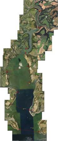
The Fal estuary is the third largest natural harbour in the world, about 18km from mouth to tidal limit (C.B. Braungardt et al., July 2011), created during the Ice Age. The estuary is classed as a ria or drowned river which formed due to sea level rise following the last ice age. It is a tide dominated estuary, with a spring tidal range of 4.6m (Port of Falmouth Development Initiative Final Report, 2009) meaning it is macrotidal. Rainfall in the South-West of England, where the Fal estuary is situated, seems to be reasonably high during the summer period (June to August) as compared to the rest of the country, indicating a high freshwater input in the area (CEH, 2008). The principle river flowing into the Fal estuary is the River Truro which is accompanied by 5 smaller rivers (Restronguet Creek, Penryn River, Pill Creek, Mylor Creek and the Tresillian). |
|
||||||||||||||||||||||||||||
|
Figure 1 - The Fal Estuary and its surrounding rivers |
The deep natural harbour means that this area is very useful as an industrial port, with ships sheltering in the Fal estuary during the recent global downturn whilst waiting for instructions as to where to take their cargo (BBC Report, Febuary,2011). The area also has an extensive mining history, stretching back to the Romano-British era (Cornish Mining World Heritage, July 2011). This can be hazardous for the surrounding marine environment, as exemplified in the Wheel Jane Tin mine incident up Restronguet Creek in 1992 where millions of gallons of contaminated waste mine water over spilled into the Carnon River (S. Ivall, July 2010) (the main freshwater input into the Fal estuary (C.B. Braungardt et al., July 2011)). Furthermore, anti-fouling paints used on ships, such as TBT, have caused imposex in gastropod species and intersex in littorinids. Pollution factors like this are highly damaging to the ecology of the area, especially as many marine organisms use the surrounding maerl beds as nurseries and habitats. Damaging the maerl could potentially cause a large-scale loss of biodiversity to the area as it can only grow in quite specific conditions and grows very slowly (up to 1mm per annum).
Water structure of the Falmouth Estuary and Surrounding Waters
Waters offshore the Fal estuary experience varied thermal stratification on a seasonal cycle with increased heating in the summer leading to a higher input to surface waters. This creates a warm buoyant surface layer which out competes mixing factors such as tides and surface winds leading to small scale shelf sea front development. These fronts occur where a warm buoyant layer and deeper cold water layer meet a homogenised mass of cool water (out flow from the Fal estuary). Water depth is a key factor which can determine tidal mixing within the continental shelf breaking fresh water front stratification generated by the fresh water input from the Fal estuary. Stratification peaks in around late June to mid-July with a high thermal input however after this period when irradiance declines, tidal action and wind fetching/lack of buoyancy contribute to mixing breaking up any stratification. With heating of the surface water mass comes front formation of the Falmouth coast which combines with fresh water fronts from the estuary input to give above average changes in physical properties along a horizontal gradients.
| RV Callista | |
| The Callista is a twin-hulled, 20m (draught 1.8m), purpose built catamaran and is the largest coastal research vessel owned and operated by the School of Ocean and Earth Science. It has an MCA Workboat Certification of category 2 (licenced to 60miles offshore) and max speed of 15kts (standard cruising speed 10kts) so it can cover up to 400nm before returning to port. The open back deck is equipped with an “A” frame capable of lifting 4 tonnes, as well as a hydraulic crane, stern winch and 150m cable meaning it is capable of deploying a variety of equipment. It also hosts a wide range of scientific equipment including a hull mounted 600Khz ADCP, fluorimeter and transmissometer, CTD and rosette system, as well as plankton nets and other instruments. In addition to the wide back deck, a wet lab and a dry lab enable accurate and efficient experimentation and data recording whilst at sea, as well as data plotting capabilities. (www.soes.soton.ac.uk/resources/boats/vessels.html) |
|
| Grey Bear Multi Purpose Vessel | |
| The FD Marine Ltd Shallow Draft Workboat Greybear is licenced to 20miles offshore but tends to remain in local Falmouth waters where it undertakes a variety of jobs in its role as a Multi Purpose Vessel. The ship has a large open foredeck capable of storing 20 tonnes of cargo and equipment, with two main deck cranes, two deck winches and a stern winch, as well as bow doors enabling a variety of different cargoes to be stored on the vessel. Limited to a speed of 7.5kts, the Greybear typically undertakes roles suited for its purpose-namely transportation and delivery of heavy equipment, cable laying, salvage as well as surveying and sampling. A computing space in the wheelhouse underneath the bridge enables underway analysis of data such as side scan sonar. A shallow draft at 1.14m when fully loaded enables the vessel to move in closer to shore than any of the SOES vessels, thereby making it a useful addition to any coastal research fleet. (FD Marine Ltd sheet) |
|
|
RV Bill Conway |
|
| The 12m, Lochin 38 Bill Conway is designed specifically for coastal research. Also certified to 60miles offshore with a standard cruising speed of 9kts (max 10) the ship is capable of a 150nm range each day. With a fully equipped wheelhouse and back deck with 750kg “A” frame and 70m trawl winch, the Bill Conway is also capable of deploying a range of scientific equipment. No specific equipment is stored on the vessel therefore allowing the ship to be outfitted for the specific role it will be undertaking at sea. |
|
| Equipment | Picture | Description | |
| Offshore and Estuarine | |||
| CTD rosette sampler including 6 Niskin sampling bottles with multiple sensors |
|
Lowered on a winch, bottles fired from computer. Fluorometer and irradiance sensor also on CTD. | |
| Plankton net with pressure sensor and messenger |
|
Mesh size of the phytoplankton net was 200 microns, attached to 30 metres of cable. | |
| Secchi Disk |
|
Standard Secchi disc attached to enough rope for all depths sampled. | |
| Light sensor |
|
There are 2 sensors associated with this piece of equipment. The first light sensor remains out of the water and is held up towards the sun to try and get the best light reading possible for air. The second is lowered into the water, 1m at a time, and the light intensity was measured at each 1m interval. | |
| ADCP (Accoustic Doppler Current Profiler) |
|
RV Callista - 600kHz and RV Bill Conway - 400kHz. The ADCPs emit a sound pulse from the transducers into the water column. These pulses are then scatter, reflected and returned to the ADCP by particles within the water. A combination of 3 or 4 sound pulses from the transducers creates a doppler shift and a profile of the water currents throughout the water column. | |
| Geophysics | |||
|
Sidescan Towfish |
|
Towed behind the boat to scan the topography of the seabed. |
|
|
The Veen grab |
|
Lowered on a winch to sample the seabed sediment. |
|
| Sieves - 1cm, 1mm and 0.5mm |
|
Used to sieve the sediment brought up from the seabed by the grab. Separates out the different size grains | |
| Plastic tray |
|
|
|
|
Video trawl |
Towed behind the boat to capture a video stream of biota and sediment of the seabed. |
||
| Wet Labs | |||
| Syringe, plastic bottle, filter container and glass fibre filter (silicon) |
 |
Used to calculate the amount of chlorophyll in the sample. | |
| Glass brown bottles (phosphate) with Lugol's iodine (zooplankton cell count) | Lugols iodine used to preserve cell structure. Glass bottles used so phosphate sample is not contaminated. | ||
| Glass bottles (dissolved oxygen) | Glass bottle to prevent oxygen loss. | ||
| 1 litre plastic sampling bottles | Used to collect seawater from Niskin bottles. | ||
| Plastic test tubes with acetone and tweezers (chlorophyll) | Filters placed in acetone in test tube and stored in freezer overnight. | ||
| Measuring cylinder | Used to measure 100ml seawater for each sample bottle. | ||
| 10ml pipette | Used for cholophyll samples. | ||
| Dry Labs | |||
| 2 computers |
|
One for the ADCP using WinRiver 2 One for the CTD profile. On the geophysics boat, the screens displayed the sidescan track. | |
| Screens |
- Screens displaying CTD profile and ship’s position on chart with depth. |
||
| Shore Lab | |||
| Fluorometer |
|
Measures fluoresence from the chlorophyll samples | |
| Nikon Eclipse E200 - compound microscope |
|
Used to identify and count phytoplankton families | |
| Nikon SMZ800 - stereo microscope |
|
Used to identify and count zooplankton classes | |
| U-1800 Spectrophotometer |
|
Used to measure phosphate and silicate concentrations by measuring the light absorbance. | |
| Dispenser pipette | Used to put a solution into every sample and standard | ||
| 4cm cell | Used to put the analysed phosphate samples into the spectrometer | ||
| Metrohm 665 Dosimat |
|
This was used to add the thiosulphate for the titration | |
| Photometric end dectector | Contains a light source and receptor and is attached to the senoscribe potentiometric recorder to monitor where the maximum amount of light penetrates the solution | ||
| Senoscribe potentiometric recorder | Visually displays the amount of penetrated light through the solution | ||
| Magnetic followers | Used to stir the dissolved oxygen titration |
|
|
|
|
|
|
|
|
|

To examine the structure of the water column from coastal waters to 20 nautical miles offshore
To locate areas with thermally stratified waters and areas which are well mixed and therefore use these to attempt to locate a front within the offshore waters
To examine the phytoplankton and zooplankton communities within the waters local to Falmouth and how they are influenced by the physical and chemical factors within the water column
On 28th June 2011 Group 1 gathered on Prince of Wales Pier at 0730GMT-a time no student should see! After embarking and a safety brief from the crew we headed away from Falmouth to the open ocean that is the English Channel. The weather for the day was sunny and bright, however the wind from the North West was reasonably strong at Force 2-3. Having previously established a plan for the day, we aimed for the first station at Black Rock (see map).
|
|
|
Figure 2 Our planned and contingency tracks and our actual track |
Our initial aim was to head straight out to sea on a course of roughly 140° true with sampling stations at 5 nautical mile intervals. Our contingency plan for the day was to take a 90° turn to port at Station 3 which was 10nm out (so we were heading off on a course of 050° true) , then continue sampling for 10nm on this heading for the final 2 stations. This would enable us to attempt to determine the location of any fronts (see earlier) and how out far any impacts reach.
However when we reached Station 2 both plans had to be adapted due to the weather conditions. Progressing further offshore the wind had longer to blow across the surface of the ocean, therefore the waves generated a longer fetch by the time they reached us thereby making them bigger. At Station 3 the waves were relatively big with Callista being significantly rocked whilst on station. Indeed several samples in the wet lab almost ended up on the floor if it weren’t for Jon catching them! Unfortunately our contingency plan was no longer viable as despite heading inland, the conditions were still too rough. A back-up plan to the back-up plan was therefore quickly established in consultation with the skipper Bill. From Station 3 we aimed for Dodman point, attempting to get close enough for around 30m of water. This should be behind any fronts in well mixed water. From here we then followed the contours down roughly on a course 140° true aiming for 60m of water. This should be in front of any fronts around Dodman point in stratified water. From here we returned to port getting back at 1530GMT in sore need of cream cakes!
|
Offshore-28.6.11 |
|||||
|
Station Number |
Time (GMT) |
Latitude (N) |
Longitude (W) |
Water Depth (m) |
Weather (cloud cover) |
|
1 |
0810 |
50°08.642 |
005°01.448 |
30.6 |
4/8 |
|
2 |
0853 |
50°05.032 |
004°56.232 |
63.0 |
4/8 |
|
3 |
1002 |
50°01.072 |
004°50.235 |
73.2 |
sunny |
|
4 |
1233 |
50°11.876 |
004°48.380 |
30.0 |
sunny |
|
5 |
1321 |
50°09.217 |
004°44.770 |
63.8 |
sunny |
|
|
|
|
|
|
|
1. Deck Methods
RV Callista arrived at each station and the deck crew prepared to deploy instruments over the side of the ship. The CTD and rosette sampler was deployed over the side using a winch and A-frame, with stabilising ropes attached to avoid danger of it swinging around and hitting the boat. It was settled at the surface so the stabilising ropes could be removed and instructions were awaited from the dry lab. The CTD was lowered to the appropriate depth and then brought back up to surface with stops at certain depths in order to close the Niskin bottles to take water samples. The CTD was raised to the surface and stabilising ropes were reattached. The CTD was brought back to the deck of the vessel and water samples were taken from the Niskin bottles. The Niskin bottles were then reset in preparation for the next station.
The plankton net (200µm mesh and 60cm diameter) and pressure sensor was attached to the winch and deployed over the back of the vessel. The net was lowered to the appropriate depth and then raised back to the surface, with a messenger being dropped at the certain depths to close the net and take a plankton sample. The plankton sample was poured into 500ml bottles.
The secchi disk was deployed over the side of vessel and lowered until it is no longer visible in the water and the depth is recorded.
The deck was then cleared and tidied and ensured that all equipment was prepared for the next station.
2. Wet Lab Methods
Phosphate. 100ml of sea water sample measured out of plastic 1L sampling bottle with a measuring cylinder and inserted into a glass bottle. Repeat for each sample depth.
Zooplankton cell count. 100ml of sea water sample measured out of plastic 1L sampling bottle with a measuring cylinder and inserted into a glass bottle containing lugo-iodine solution. Repeat for each sample depth.
Dissolved oxygen. Use plastic tubing to fill clear glass bottle with water sample directly from the Niskin bottle. Pipette 1ml of manganese chloride and add to sample, note release solution well below the sample meniscus to avoid displacement of reagent. Pipette 1ml of alkaline iodide and add to sample. Invert and lightly shake and place in a water filled container. Repeat for each depth sample.
Silicon. A clean syringe was used to take a 50ml sample which was then filtered through a 40 micron mesh glass fibre filter into a numbered plastic bottle and refrigerated.
Chlorophyll. The filter used in the silicon filtration was removed and placed into a numbered test tube containing 6ml of 90% acetone and refrigerated.
3. Dry Lab Methods
- The first ADCP transect was taken at station 1; once the vessel left station 1 a new transect was opened, which automatically saved the transect taken at the station. On arrival at the next station another new transect was opened, saving the previous transect from between stations. This process was repeated at arrival and departure of each station.
- A new file was created everytime the CTD was deployed, after the down cast the profile was used to determine which depths to take water samples at. By following the up cast the CTD was raised to required depths at which niskin bottles were fired using controls on the computer software; in the event of a mis-fire another bottle was closed. Each file was saved when the CTD was retrieved from the water.
4. Shore Lab Methods
Phosphate analysis - The
phosphate analysis was done using the standard method (Parsons
T. R. Maita Y. and Lalli C. (1984) “ A manual of chemical and biological methods
for seawater analysis” 173 p. Pergamon).
Silicate analysis -
Add 2ml of
Molybdate solution was added to the 5ml of respective filtered seawater, this
was left for 10 minutes before 3ml of Mixed Reducing Agent (MRR) was added again
using a pipette with a clean tip attached. The cap was secured to the tubes and
each one given a gentle shake by hand. They were then left for 2 hours. The 90ml
of MRR was made comprising of 30ml of Metol Sulphite, 18ml of Oxalic Acid, 18ml
of Sulphuric Acid and 24ml of Milli-Q Water.
After 2 hours the absorbance of the Silicon was measured using a U-1800
spectrophotometer set at a wavelength of 810nm. The samples were each
individually transferred from the capped tubes into a 4cm cell before being
placed into the spectrophotometer and absorbance measured. Between each
measurement the 4cm glass cell was rinsed out with Milli-Q water.
Dissolved Oxygen Analysis - 1ml of sulphuric was added to the bottles containing the water sample and Winkler reagents prepared on the vessel in the wet lab; this dissolved the precipitate. A magnetic follower was added to stir the sample prior to titration with the thiosulphate solution. The end point occurred at the point where the maximum amount of light was penetrating the sample, the progress of which was monitored using the Senoscribe. This procedure is as per the altered Winkler method described in Bryan et al (1976).
Chlorophyll Analysis - The filters from the silicate filtration which had collected the chlorophyll had been stored in acetone and kept in a freezer overnight. The samples were removed from the freezer and the filters were removed from the acetone. The acetone which had extracted the chlorophyll from the filters was then poured into a testtube and put into the chlorophyll measuring machine. The amount of chlorophyll in each sample was recorded and multiplied up so it was representative of the 50ml sample.
ADCP Analysis - Input raw data into WinRiver II.
CTD Analysis - Input raw data into Excel. Separate into columns, copy into Sigmaplot and create simple straight line graphs.
Phytoplankton and Zooplankton
Analysis - Using phytoplankton microscopes and zooplankton microscopes
respectively, we counted and identified the different families of phytoplankton
and the different classes of the zooplankton samples.
|
|
|
|
|
|
|
|
|
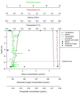
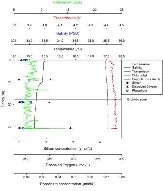
| Figure3.1 Station 1 | Figure 3.2 Station 2 |
|
|
|
|
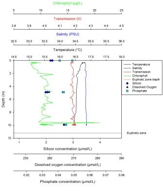
Silicon has a maximum of 3.05µm at 9m and a minimum of 2.64µm at 27m. It is present at low levels at the surface, then peaks at about 8m depth before becoming depleted once more at depth. From 1-9m, the dissolved oxygen steadily declines from 279µmol/l, then has a much sharper decline below 9m to 250µmol/l at 27m. Phosphate increases sharply from the surface (0.169µmml/l) to 9m before increasing more steadily from 9m to 27m where there is a maximum of 0.255µmol/l. The LUP shows a maximum value of -0.15 AU at the surface which steadily decreases with depth to -0.32 AU. Fluorescence shows an increase in value from the surface to 9m where it then remains constant with depth. Only the trend is described here as no values were obtained due to problems with the chlorophyll measurements. The maximum temperature was found at the surface at 13.5oC which steadily decreased until 3m where the thermocline developed to a depth of 6m. From 6m to 12m the temperature decreases to 12.5oC, after which the temperature stays constant. At this station there was interference at depth. This station was also the closest to shore. |
Silicon has a maximum of 4.54µmol at 39m and a minimum value of 1.8µmol at 10m. This nutrient was initially depleted in the surface waters but then steadily increased in concentration with depth. The maximum dissolved oxygen was found at 10m and was 275µmol/l. This decreased steadily with depth until the minimum value of 1.8µmol/l was reached at 39m. Phosphate concentrations showed a sharp linear increase from 10m, where the minimum value of 0.15µmol/l is found, to 30m after which there is a less sharp but steady increase. The maximum value is found at depth and is 0.49µmol/l. The LUP has a maximum value of -0.1 AU at the surface then steadily decreases until 38m to the minimum value of -0.25 AU. Here the trend shows an increase until 57m to a value of -0.19 AU. Fluorescence was lowest at the surface, with two peaks at 28m and 57m. The largest peak was seen at 28m. There was also a lot of noise in this profile. The temperature reached a maximum of 14.2oC at the surface and a minimum of 11.3oC from 38m to 56m. The temperature in this profile remained constant until the thermocline at 9m. This continued until 11m where it broke down and the temperature steadily decreased until 38m where it became constant once more. |
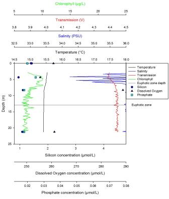
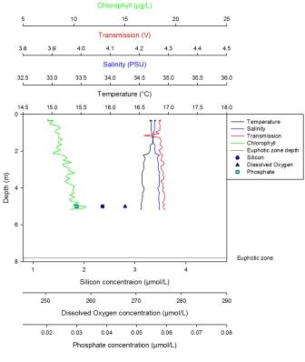
| Figure 3.3 Station 3 | Figure 3.4 Station 4 |
|
|
|
|
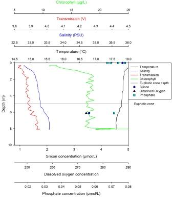
The minimum value for silicon concentration was 13µmol at 12m with the silicon profile decreasing linearly with depth. The maximum value for silicon is 48µmol at 48m. The dissolved oxygen profile decreases steadily from 12m (the maximum value, 262µmol/l) until 20m. Here the decease becomes sharper until 49m, where the minimum value, 242µmol/l, is reached. Phosphate has a maximum concentration of 0.352µmol/l at 49m and a minimum concentration of 0.10µmol/l at 12m. The profile shows a linear increase from the lowest values at the surface to the maximum values at depth. The LUP has a maximum value of -0.05 AU at the surface. The LUP profile shows a decline to 32m, whereupon the decrease becomes sharper. This may be due to the shadow of the vessel, and the LUP value stays constant and very low until 40m. At this point it increases to a point in line with the expected LUP profile. From here on it decreases steadily until 70m. Fluorescence is low at the surface but increases with depth until 20m. From 20m to 22m a sharp decrease occurs. From 22m to 70m fluorescence remains constant apart from small fluctuations. From the maximum temperature at the surface (14.1oC) to 10m depth the temperature decreases steadily. There is a strong thermocline between 10m and 20m after which a weak decrease occurs down to the minimum value of 11.4oC at 70m. |
The maximum concentration for silicon is 2.38µmol at 22m with a minimum value of 1.89µmol at 8m. From the surface the profile shows a decrease down to 8m at which point a linear increase occurs until 22m. Dissolved oxygen has a maximum of 258µmol/l at 8m then decreases steadily until the minimum value of 247.5µmol/l at 22m. The maximum concentration for phosphate is 0.122µmol/l at 2m depth. It steadily decreases to 10m, where the decrease becomes sharper and continues to the minimum value of 0.076µmol/l at 22m. The LUP decreases steadily from the maximum value of -0.01 AU at the surface until the minimum value of -0.21 AU is reached at 27m. Fluorescence shows gradual increase with depth following the salinity profile. Temperature reaches a maximum at the surface of 14.2oC and a minimum at 27m of 13oC. The temperature profile decreases down to 10m at which point a weak thermocline occurs to 15m depth. After this there is a slight decrease down to 27m. |
| Figure 3.5 Station 5 | |
|
|
Nutrient data starts at 15m for station 5. The silicon increases sharply from a minimum concentration of 2.51µmol at 15m to the maximum of 3.3µmol at 24m before decreasing steadily to 27m. The dissolved oxygen decreases sharply from a maximum of 274µmol/l at 15m to 24m, where there is a steady decrease, reaching the minimum value of 228µmol/l at 27m. The maximum concentration for phosphate is 0.37µmol/l at 27m and the minimum concentration is 0.1µmol/l at 15m. This profile follows the silicon profile, showing a sharp increase nearer the surface and a steady decrease to the bottom of the profile. The LUP shows a maximum value at the surface of -0.1 AU. The LUP remains constant from surface to 32m depth after which there is a horizontal decrease from -0.28 AU to -0.98AU. The profile shows a vertical trend between 32m and 47m, remaining constant at -0.98 AU. The minimum value observed, excluding the shadow is -0.28 AU at 32m. After 47m there is a horizontal increase to -0.2 AU. Fluorescence increases steadily with depth until a maximum between 18m to 30m, after which the increase becomes less significant until a depth of 60m. The temperature maximum occurs at the surface at 14.45oC. The temperature profile remains constant until 10m, at which point there is a strong thermocline down to 30m. This is where the minimum value occurs at 11.4oC. The profile remains constant from 30m to the bottom. |

| Figure 4.1 Zooplankton Legends | |||
|
|
|||
| Figure 4.2 Station 1 - 21m to surface | Most abundant | Figure 4.3 Station 1- 21m to surface | Most abundant |
|
|
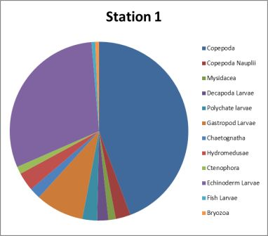
Hydromedusae 38%
Copepoda 19%
Polychaete larvae19% |
|
Copepoda 31% Polychaete larvae 31% Hydromedusae 16%
|
| Figure 4.4 Station 2 - 27m to surface | Figure 4.5 Station 2- 27m to surface | ||
|
|
1. Hydromedusae 47%
2. Chaetognatha 15%
3. Echinoderm larvae 8% |
|
1. Hydromedusae 47% 2. Copepoda 12% 3. Echinoderm larvae 8%
|
|
It is unlikely for a sample containing loads of chaetognaths (i.e. bottle 2A) to also contain loads of copepods as the juveniles feed on copepod nauplii (Baier et Purcell, 1997). |
|||
| Figure 4.6 Station 3 - 22.5m to surface | Figure 4.7 Station 3 - 22.5m to surface | ||
|
|
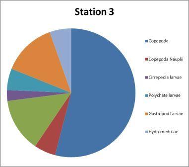
1. Hydromedusae: 48% 2. Copepoda: 13%
3. Fish Larvae: 9% |
|
1. Hydromedusae: 58% 2. Fish Larvae: 13% 3. Copepoda: 11%
|
|
This may be due to the distance from the shore, which was greatest at this station. It is possible the area in which we were sampling was a nursery ground. Note also that chaetognaths which eat fish larvae (Baier et Purcell, 1997) are not highly abundant here. |
|||
| Figure 4.8 Station 4 - 20m to surface | Figure 4.9 Station 4 - 20m to surface | ||
|
|
1. Hydromedusae: 56% 2. Polychate larvae: 11% 3. Copepoda: 10% |
|
1. Hydromedusae: 35% 2. Ctenophora: 22% 3. Copepoda: 13% |
| Figure 4.10 Station 5 - 29.3m to 15m | Figure 4.11 Station 5- 15m to surface | ||
|
|
1. Chaetognatha: 33% 2. Echinoderm larvae 11%
Appendicularia 11% Copepoda: 11% |
|
1. Hydromedusae: 39% 2. Cirripedia larvae: 19% 3. Copepoda: 15%
|
For sites one to four the mesh on the net was clogged with organic detritus so may not have filtered properly. By station five there was less organic matter, however the collection bottle was swollen and water was lost from this sample. These errors may have had an effect on the samples, but as they were present in most of the samples, this effect cannot be clearly determined. The plankton net could not be closed from stations one to four due to a faulty messenger, so a drag of the entire water column was taken. This means upper and lower water column structure can only be determined from site 5.
The upper water column appears to be dominated by hydromedusae; at site 5 hydromedusae were much more prevalent in the upper water column net than the lower water column, which was dominated by chaetognatha. There appears to be little overall difference in zooplankton present in the well mixed sites (one and four) and the stratified sites (two, three and five). Chaetognathans appear to do well at depth as they are highly abundant in the lower water column of station five and at station two; which is one of the deeper station.In terms of total zooplankton numbers bottles 1A and 5A have relatively fewer numbers while 5C has relatively higher numbers, the lower numbers are an order of magnitude less than the highest. In stratified waters (station 5) above the thermocline there are much higher amounts of zooplankton, this is likely to be due to phytoplankton growth around and above the thermocline.
Hydromedusae - Research into the Atlantic hydromedusan Aglantha digitale by Takahasi and Ikeda (2006) linked this species to copepods and chaetognaths as its food resource. If this is the same species of hydromedusan present in our samples then it may explain the relationship between copepods and hydromedusan abundance seen in in sample bottles from station 1.
Copepods - These play an important role in structuring food webs, their growth is limited by food (phytoplankton and microzooplankton) availability and predation; therefore they are indirectly limited by factors controlling phytoplankton such as light and nutrients. Their shape is relatively constant throughout the order and is likely to have evolved as a predator escape mechanism as they can escape quickly from, and sense any oncoming prey. (Kiorboe, 1998). Species are present around Plymouth across the year, some may spawn up to 5 times a year and there is a succession of species present. (Digby, 1950). However, a significant long-term increase in copepod community species richness has been observed and its maximum annual value was significantly related to annual average sea surface temperature. A study by Harris (2010) confirmed that there is a summer spawning season and also one in the autumn. The historical trend for increasing autumn spawning has continued. The mean spawning temperatures were 12.68C and 14.58C for the summer and autumn seasons, respectively. Heterotrophic dinoflagellates dominated the protozooplankton in June, but ciliates dominated the rest of the seasonal cycle. This study demonstrates the importance of protozooplankton as a food source for copepods in this coastal ecosystem
Chaetognatha- This species lay and wait ambush predators on other zooplankton and fish larvae, they are therefore important as predators and competitors of larval fish. Small chaetognaths feed on copepod nauplii and tintinnids, progressing to copepods and other large prey as they grow. Chaetognath predation has been shown to significantly affect populations of copepods or larvaceans, and copepods have been found to be their main prey in many studies. (Baier, 1997; Harris,2010)

| Number of cells per m3 | |||||||||||||||
| Station 1 Depths (m) | Station 2 Depths (m) | Station 3 Depths (m) | Station 4 Depths (m) | Station 5 Depths (m) | |||||||||||
| Phytoplankton Species | 1.3 | 9.1 | 27 | 9.58 | 31.33 | 39.24 | 11.9 | 19.5 | 47.4 | 1.4 | 8.6 | 21.14 | 15.5 | 23.5 | 27.2 |
|
Cylindrothera |
1x10⁷ | 6x10⁷ | 1x10⁷ | ||||||||||||
|
Chaetoceros |
5.4x10⁸ | 2.9x10⁸ | 4.2x10⁸ | 9x10⁷ | 1.6x10⁸ | 1.6x10⁸ | 2.5x10⁸ | 2.6x10⁸ | |||||||
|
Laudericae |
6x10⁷ | 1.1x10⁸ | 2.x107 | 9x10⁷ | 3x10⁷ | 8x10⁷ | |||||||||
|
Rhizosolenia |
2.6x10⁸ | 2.8x10⁸ | 1.4x10⁸ | 4x10⁷ | 1.2x10⁸ | 2x10⁷ | 4x10⁸ | 6x10⁷ | 1.4x10⁸ | 9x10⁷ | 1.2x10⁸ | 2.7x10⁸ | 1.4x10⁸ | 7x10⁷ | |
|
Karenia mikimotoi |
1x10⁷ | ||||||||||||||
|
Guindardia |
6x10⁷ | 3x10⁷ | 1.3x10⁸ | 6x10⁷ | 6x10⁷ | 7x10⁷ | 2x10⁸ | ||||||||
|
Thalassiosira |
4.4x10⁸ | 1.3x10⁸ | 1.4x10⁸ | 3.1x10⁸ | 2x10⁷ | 1.3x10⁸ | 1x10⁷ | 1.1x10⁸ | 1.6x10⁸ | 1x10⁸ | |||||
|
Coscinodiscus |
2x10⁷ | 2x10⁷ | 1x10⁷ | ||||||||||||
|
Leptocylindrus |
1.3x10⁸ | 5.1x10⁸ | 1.1x10⁸ | ||||||||||||
| Stephenopyxix | 6x10⁷ | ||||||||||||||
|
Diatom |
2x10⁸ | 6.3x10⁸ | 2x10⁷ | 4x10⁷ | 1.5x10⁸ | 5x10⁷ | 2x10⁸ | ||||||||
|
Detonula |
1.1x10⁸ | 5x10⁷ | |||||||||||||
|
Ceratulina |
4x10⁷ | 1x10⁷ | 7x10⁷ | ||||||||||||
|
Skeletonema |
1.8x10⁸ | 8x10⁷ | 1.8x10⁸ | 1x10⁷ | |||||||||||
|
Bacillaria |
2x10⁷ | 8x10⁷ | 1.5x10⁸ | ||||||||||||
|
Protoperidiniaceae |
1x10⁷ | ||||||||||||||
|
Eucampia |
1.4x10⁸ | ||||||||||||||
|
Ceratulina |
1.5x10⁸ | ||||||||||||||
|
Bacteriastrum hyalinum |
1.1x10⁸ | ||||||||||||||
|
Ceratiaceae |
1x10⁷ | ||||||||||||||
|
Naked Dinoflagellate (Pyrophacus) |
6x10⁷ | 1x10⁷ | |||||||||||||
|
Prorocentrum |
5x10⁷ | ||||||||||||||
|
Armoured Dinoflagellate |
1x10⁷ | 5x10⁷ | 4x10⁷ | ||||||||||||
|
Dactyliosolin |
1.2x10⁸ | ||||||||||||||
|
Hemiaulus |
1.1x10⁸ | ||||||||||||||

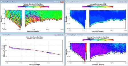
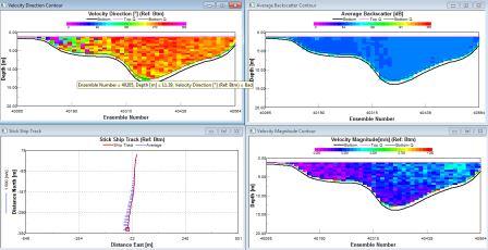
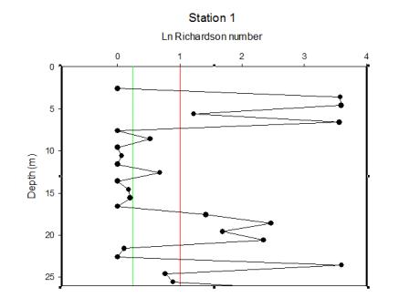
| Figure 5.1 Station 1 | Figure 5.2 Station 1 Richarson Number | Figure 5.3 Between stations 1-2 |
|
|
 |
|
| The water direction is heading south throughout the surface half of the water column and in a northerly direction from 15m and below. There are high amounts of back scatter of about 110db in the surface 5m, then low amounts throughout the rest of the water column between 69 and 75db. The velocity magnitude is low at depth (0.001-0.1m/s) with occasional spikes of higher velocities in the surface 5m. | Between about 2m and 6m depth, there is stability within the water column. From 6 to 17m, there is an area of mixing within the water column showing instability. Below this, the water mass becomes more stable with brief pockets of instability. |
The water direction is predominantly SW (confirmed by ship track). There are high amounts of back scatter (90db) in the surface 5m and at depths around 50m. The intermediate waters are generally lower (80db). The velocity is generally low, between 0.01 and 0.1ms-1 at the start of the transect throughout the water column. Progressing out to sea the velocity increases starting at the surface and increasing throughout depth until it is universally higher at about 0.3ms-1. |
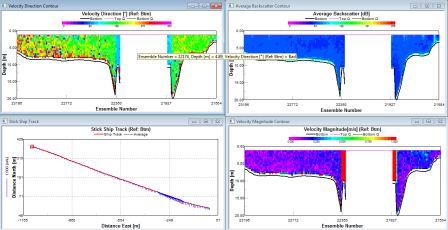
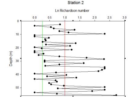
| Figure 5.4 Station 2 | Figure 5.5 Station 2 Richardson Number | Figure 5.6 Between stations 2-3 |
|
|
 |
|
|
The water direction is consistently SW throughout the water column. There is low back scatter (73db) at depth with very low levels at some mid waters (58db). In the surface 10m there is high back scatter between 100-115db. The velocity is generally low throughout the water column between 0.1-0.3ms-1, but with some slight increases to 0.35ms-1 at the surface and at the benthic boundary indicating wind and tidal mixing. |
The water mass of station 2 fluctuates regularly between stable and unstable structures. Stable, stratified water alternates with larger areas of mixing. This gives an overall impression of high mixing within this water column. |
The water direction is generally SW. The back scatter is high at the surface and at depths of 60m (85-90db) whereas the intermediate waters have comparatively low back scatter of 75db. The magnitude is consistently mid level of 0.35ms-1 at the surface and intermediate waters at the start of the transect. The velocity then decreases in the mid waters first followed by the rest of the water column with levels reaching 0.15ms-1. |
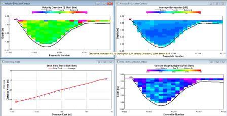
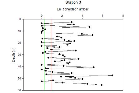
| Figure 5.7 Station 3 | Figure 5.8 Station 3 Richardson Number | Figure 5.9 Between stations 3-4 |
|
|
 |
|
|
The water direction is generally SW again, with high backscatter at the surface (110db). Medium levels of backscatter were detected at depth (50-75m; 75-80db), with low values in intermediate waters of 70db. The magnitude is sporadically med level at depth and at the surface with levels reaching 0.4ms-1, intermediate waters at consistently lower speeds of water movement (0.07-0.2 ms-1; 20-50m) |
Station 3 is mostly stratified with isolated layers of internal mixing around 10 and 42m depth. |
Surface to intermediate waters have a westerly direction (verified by the ship track), whilst deeper wates have a northerly direction. The backscatter is medium of 90db at surface levels and at depths of 40-60m. low levels of 75db in the mid waters, with very low levels of 68db just below the surface high. The magnitude is low throughout between 0.01 and 0.3ms-1. |
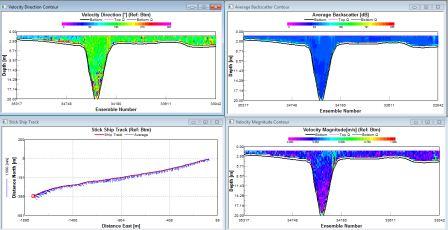
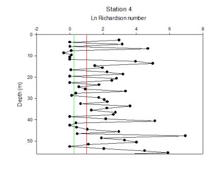
| Figure 5.10 Station 4 | Figure 5.11 Station 4 Richardson Number | Figure 5.12 Between stations 4-5 |
|
|
 |
|
|
The direction at the surface and at depth is SW, whilst a plume of north flowing water dominates the intermediate levels. The backscatter is medium to high at surface waters (110db), low values of 65db at depth with levels of around 75db throughout the mid water. There is a gradual decrease throughout the water column. Velocity is high at the surface between 0.4 and 0.5 ms-1, with levels of 0.8ms-1 or less at intermediate to deep waters, with very low levels below 15m (0.03 ms-1). |
Station 4 also has a mostly stratified water column with some layers of internal mixing at about 8 and 43m depth. |
The direction of the surface waters is SW, around 20m this becomes a N direction with deep waters flowing in an Easterly direction. There is a SW plume towards station 5 in mid-waters. The backscatter has medium levels of 85db at the surface, with levels of 75-80db in mid-waters. At a depth of 40m there is a value of 68db increasing back towards 75db below 40m. Magnitude is intermediate at the surface with levels of 0.2 ms-1. Below 15m there are values of 0.15 ms-1 or less, with this increasing towards 0.2 ms-1 at the benthic boundary. Between 20-40m there are very low levels of movement of 0.05 ms-1. |
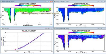
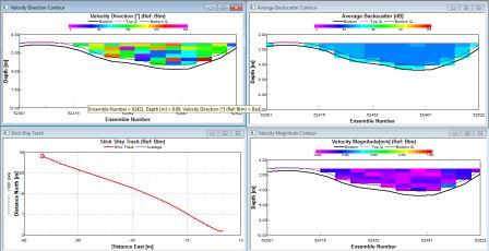
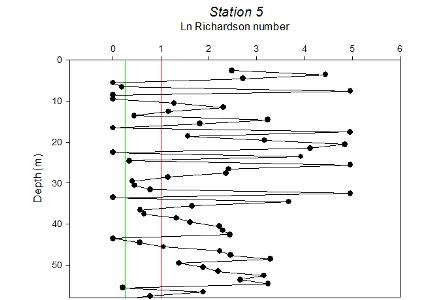
| Figure 5.13 Station 5 | Figure 5.14 Station 5 Richardson Number | Figure 5.15 Between stations 5-Midway back |
|
|
 |
|
|
The direction of water movement is SW between surface at 20m, at 20m there is again a northerly direction, with east flowing water below it. Backscatter is high at the surface (110db) and then low throughout the rest of the water column (73db). There is a medium plume at the end of the track around 30m with values of 85db. Magnitude is 0.4ms-1 at the surface, with very low levels throughout the rest of the water column. There is again a small increase at the benthic boundary. |
Station 5 is stratified in some layers alternating with layers of internal mixing. The stable layers are highly stratified. |
SW flowing waters are found at the surface, with a north direction at 10m, followed east direction below this. The backscatter is 90db in the surface 2m, at 20m there is a low of 75db (with decreasing levels in between), whilst below 20m levels increase back up towards 90db by the bottom. There is a plume of low backscatter mid-way and at the end of the track, with levels between 69-75db throughout the water column. The magnitude is generally low throughout the water column with some occasional medium level values of 0.25ms-1. |
|
|
|
|
|
|
|
Station 1
Station 1 has a well mixed column which is indicated by a weak thermocline between 5 and 12m depth. There are higher salinities in the deeper waters, which is consistent with the more saline oceanic water mass intruding into fresher estuarine waters; this can be seen on the ADCP profile where there are 2 distinctive water masses. The potential chlorophyll maximum is at around 10m depth which is within the expected euphotic zone which potentially shows the phytoplankton are predominantly in the surface waters where there is sufficient light for photosynthesis. In addition, chlorophyll may decrease below 10m due to consumption by predators, such as zooplankton, combined with a lack of replenishment of population by growth. This is not completely reliable however, as the chlorophyll is just an indicator of phytoplankton concentrations and not a proxy for production. Furthermore, the data from the samples and from the lab results may not be accurate or reliable due to instrumental and analytical errors. The silicon data shows a trend that indicates an increase at the same rate as the chlorophyll between 0-10m, with both of them decreasing with depth. This is inconsistent with the expected theory of silica depletion by diatom uptake. This could be due to recycling at the thermocline, thus the silica maximum is created at the same rate as the diatom maximum. The silicon trend could be anomalous as it is expected that silicon should decrease with diatom increase. This could be explained by a lack of silicon utilising phytoplankton (diatoms), so silicon is not taken up as much as other growth nutrients. Within the surface water, phosphate shows depletion. At the next depth that was sampled, the values indicate that phosphate would increase slowly in the first 10m, then at a faster rate in deeper waters. This could be explained by it not being used up due to less photosynthesis occurring in deeper, less light saturated waters. It could also be more abundant in deeper waters due to cells dying, decomposing and sinking down past 10m where the dissolved phosphate is then remineralised. The dissolved oxygen concentration at this station is predictably higher at the surface due to atmospheric input and then lower at depth due to aerobic respiration conducted by bacterial decomposition. The light at this station also decreases with depth because light is absorbed and scattered in the water column by sediment and other particulates.
Station 2
Station 2 is a partially mixed water column exhibiting a thermocline which is either developing or diminishing. The thermocline has 2 parts to it; the first being more distinctive than the second with a sharp decrease in temperature occurring between 8 and 10m, and a more gradual decrease between 10 and 30m. If the thermocline is developing, it indicates summer heating, which causes stratification to arise due to warmer, lighter water overlying colder, denser water. If the thermocline was diminishing, this could indicate recent stormy weather which would cause a break down in the water column structure. A halocline appears at approximately the same depth as the thermocline between 10 and 30m deep. There are a lot of salinity spikes in the data that is most likely due to lags in the CTD and to the strong temperature changes. The fresher surface layer could be explained by recent precipitation in the area. Summer waters are expected to be highly stratified; however, due to recent stormy weather and high winds from the southwest, the water column is more mixed than usual for this time of year. At the depths that were sampled, the dissolved oxygen shows a decrease with depth due to aerobic respiration as mentioned previously. Light decreases because of reasons also mentioned before. The trends suggest that there are higher nutrient levels in the second part of the thermocline, which corresponds with a potential chlorophyll maximum at a depth of 30m. Based on the depths samples, phosphate shows a rapid decrease at the chlorophyll maximum due to increased consumption by phytoplankton at this point. This cannot be totally verified because of the small number of samples that have been taken through the water column. This means there are not enough data points to accurately determine nutrient trends. The euphotic depth as taken by the secchi depth is shown to be 15m which is much shallower than expected considering the probable chlorophyll maximum is at 30m. This could possibly be because of cloud cover or the shadow of the boat.
Station 3
The euphotic zone at station 3 is consistent with the likely chlorophyll maximum, based on the limited depth samples, at 20m depth displayed on the CTD profile. Phosphate and silicate show a trend that could be interpreted as a steady increase, particularly below 20m, because of the perceived decrease in phytoplankton. There is strong stratification shown by a distinctive shallow thermocline from 0-20m, this is supported by data from the ADCP profiles and the high Richardson Numbers which were calculated, showing that the water column is stable. The thermocline can further explain the assumed chlorophyll maximum at this depth. This is where phytoplankton generally bloom due to slightly higher inputs of nutrients at this depth from some mixing occurring between the surface and bottom layers. Surface waters at this point in summer have already being stripped of nutrients due to previous phytoplankton blooms. Furthermore, phytoplankton cannot migrate into deeper nutrient rich waters because of resultant warmer, more buoyant waters on the surface. Phytoplankton populations could also be affected by zooplankton grazing. Despite the trends of chlorophyll increasing in the surface 20m, the dissolved oxygen concentrations show a decrease, from the samples taken, which could be explained by increased respiration rates from zooplankton grazing in this chlorophyll rich area. In the mid-layers of the water column, water flows in a south westerly direction with surface waters flowing in a southerly direction as a result of the wind coming from the North and possible deflection. Owing to the fact that this mid-layer change in direction is not supported by CTD changes in temperature or salinity, it is not possible to say with certainty that this is a completely separate water mass or current.
Station 4
Station 4, as seen by the limited samples collected, illustrates an increase in chlorophyll possibly relating to a decrease in phosphate concentration. This is likely to be because of phosphate aiding the growth of phytoplankton as it is a cofactor of chlorophyll. The potential chlorophyll maximum appears to occur at about 20m, which is within the euphotic layer of 28.5m, as shown by the secchi disk depth. The CTD data shows a very slight decrease of irradiance with depth and has appeared to limit phytoplankton growth. Silicon shows a tendency to decrease as a result of diatom uptake at 8.6m, which is consistent with the thermocline at about 12m, and then increases with depth. Dissolved oxygen shows a trend that could be described as a decrease with depth, which is as expected. Silicon though, with the data that was collected, shows an increase with depth after 10m, which is around the same depth as the weak thermocline that can be seen from the CTD data. The decrease in silicon in the upper part of the water column can be likely to be caused by the increase in chlorophyll.
Station 5
The CTD data for this station shows there to be a massive anomalous decrease in light intensity from about 35 to 45m depth. This has been attributed to the boat overshadowing or rosette sampling apparatus drifting under the boat, thus causing a very sharp, large loss of light. This should not particularly affect the other data taken. This station also shows a large increase of silicon with depth, which like in station 4 can be attributed to the addition of silicon from the cliffs. The chlorophyll maximum is consistent with the eutrophic zone as seen by the secchi depth of…The depth of the euphotic zone also coincides with the depth of the thermocline, showing an increase/decrease with depth of station (closer to coast?). There is a northern boundary due to shear between the two water masses.
Phytoplankton Interpretations
It has been seen that there are relatively small numbers of dinoflagellates compared to numbers of diatoms which is uncharacteristic of this time of year. On the north-west European continental shelf, the diatom bloom occurs in spring followed by a dinoflagellate dominated water column in the summer; autumn also holds another peak in diatoms (Maddock et al, 1981). Holligan and Harbour (1977) also state that dinoflagellates dominate at the thermocline between June and August prior to a second diatom bloom in September when the thermocline erodes. The phytoplankton counts from the offshore samples are no representative of these ideas; however, it is possible that stormy weather during early June has had an impact on the stability of the water column in these coastal waters.
The diatoms are present in spring and autumn waters due to full vertical mixing which stabilises the water column; the high winds in the previous months have meant that the water has stayed more mixed and less favourable to the thermocline residing dinoflagellates. The data does however show numbers of both diatoms and dinoflagellates coinciding, this is due to intermediate stratification; as you can see in above CTD profiles some of the stations are more stratified than others, in areas such as these there are other outcomes of competition (Jones and Gowen, 1990). The phytoplankton counts show the highest density of dinoflagellates at station 5; this station was on the stratified side of a frontal system with station 4 on the mixed side. There appears to be a larger number of athecate (naked) than thecate (armoured) dinoflagellates which also appears consistent with stormy weather; thecate dinoflagellates have the ability to shed their theca during periods of heightened stress, the environmental stress from storms may have caused this. Although some of the dinoflagellates were unidentified, SAHFOS (http://www.sahfos.ac.uk/taxonomy/phytoplankton.aspx) showed that there are normally high densities of the ceratium, protoperidinium and scrippsiella; these may have been included in the samples that were collected.
The highest abundance appeared to be the families chaetocerotaceae, rhizosoleniaceae and thalassiosiraceae which follows the distributions found on the Sir Alistair Hardy Foundation of Science website which display high chaetoceros and thalassiosira genus densities. The SAHFOS site also showed high density of Lauderia annulata which isn’t immediately apparent from the results. Rhizosolenia is described as being widespread throughout the world’s oceans with some restrictions varying between species (Guillard and Kilham, 1977).
Thalassiosira are only abundant at the offshore stations at depth, whereas they were identified in all samples closer to shore; these may be due to variations in irradiance. In Strzepek and Price (2000) it was seen that thalassiosira cells contained 4 times more iron when light-limited and held higher chlorophyll a concentrations at intermediate irradiance. This explains why they were present at depth offshore; the thalassiosira were present at the shallow depths near shore possibly because of iron leaching from the land or reduced irradiance due to turbidity from sediments.
Conclusions
The stations nearer the shore (Station 1 and Station 4) were well-mixed, indicating that they were on the shore side of any fronts. The stations further away from shore (Station 2, Station 3 and Station 5) were all stratified, indicating that they were on the ocean side of any fronts. Where surface or near-surface samples were taken, phosphate and silicate were depleted, while dissolved oxygen was high. This, combined with high surface chlorophyll levels, indicates that there were a large concentration of phytoplankton in the surface waters. Chlorophyll spikes on the thermocline of Station 2, Station 3 and Station 5 indicate high phytoplankton on the thermocline, which is consistent with the depleted surface nutrients and water column stratification.
|
|
|
|
|
|
|
|
|
Survey the maerl beds in the Special Area of Conservation (SAC)
Explore the extent of growth of the maerl beds
Gauge the biodiversity of the SAC
Analyse the sediment composition of Falmouth Bay

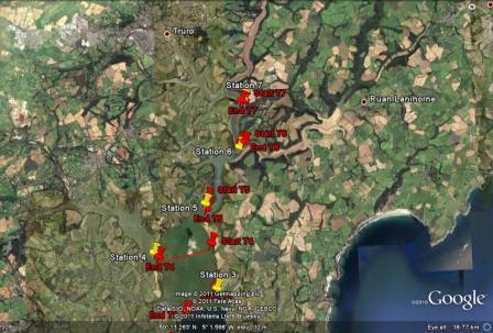
The plan for the geophysical survey was to head east from the harbour until we left the conservation area. We would then travel to just past St. Anthony’s head, a point directly north of the seabed feature known as the Old Wall and run an echosounder transect to determine the general features of the area. We would then run sidescan transects down this transect line and then either side of the first transect line, observing the results to determine where we wished to use the grab to sample the sea bed.
|
|
|
| Figure 6.1 Position of sidescan tracks | Figure 6.2 Close up position of sidescan tracks and grab sites |
We followed this plan initially. However, the first sidescan transect showed that the sea bed around the Old Wall was almost entirely rock, so we would not be able to use the grab to sample the sea bed. Instead of continuing with the initial plan, we changed our survey area to an area west of our initial survey area. We ran five short east-west sidescan transects and determined two grab sites. Once all five transects were completed, we performed two grabs and sieved the sediments before returning to the harbour.
|
Geophysics-1.7.11 |
|||||
|
Station Number |
Time (GMT) |
Latitude (N) |
Longitude (W) |
Water Depth (m) |
Weather (cloud cover) |
|
Start of Ecosounder route |
0745 |
50°08.300 |
005°00.000 |
|
1/8, sunny |
|
End of Ecosounder route |
0830 |
50°07.050 |
005°01.750 |
|
1/8, sunny |
|
|
|
Northings |
Eastings |
|
|
|
Start of Transect 1 |
091102 |
28574 |
183400 |
|
1/8, sunny |
|
End of Transect 1 |
091258 |
28589.7 |
183170 |
|
1/8, sunny |
|
Start of Transect 2 |
091554 |
28659 |
183190 |
|
1/8, sunny |
|
End of Transect 2 |
091758 |
28660 |
183408 |
|
1/8, sunny |
|
Start of Transect 3 |
092148 |
28788 |
183391 |
|
1/8, sunny |
|
End of Transect 3 |
092338 |
28793 |
183170 |
|
1/8, sunny |
|
Start of Transect 4 |
093355 |
28879 |
183182 |
|
1/8, sunny |
|
End of Transect 4 |
093548 |
28889 |
183408 |
|
1/8, sunny |
|
Start of Transect 5 |
094039 |
28986 |
183399 |
|
1/8, sunny |
|
End of Transect 5 |
094238 |
28971 |
183165 |
|
1/8, sunny |
|
Grab Site 1 |
102301 |
28982.9 |
183369 |
21.7 |
1/8, sunny |
|
Grab Site 2 |
104002 |
28561.5 |
183372 |
21.4 |
1/8, sunny |

Now Falmouth Bay is classed as a SAC, EU legislation protects the Maerl in several ways. For example Annex I Habitat, ‘sandbanks which are slightly covered by seawater all of the time’ and ‘shallow inlets and bays’, both include maerl and are protected by the laws. The maerl beds are a UK Biodiversity Action Plan habitat with the objectives of maintaining the geographical range and the variety and quality of the maerl beds and associated plant and animal communities in the UK. Monitoring Falmouth Bay for the status of the maerl beds is needed and is completed by using the following parameters; dimensions, density of covering epiphytes, sediment, changes in water quality, temperature and salinity, proportions of living to dead maerl in surface layers and species diversity within the biotope.
 |
| Figure 7 Different types of maerl - free living maerl and encrusting maerl |

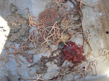
Ophiuroidea are a class of Echinodermata also known as brittle stars which inhabit a wide range of habitats across the globe (Buchanan 1964). Their benthic lifestyles offer several niches where the main determining factor between species specialization is feeding method. Every possible feeding method has been hypothesized for ophiuroids (Buchanan 1964) thus they are highly diverse and adaptive however there are two dominate methods. Suspension feeders raise their arms to trap particulates and phytoplankton within the water column thus are highly responsive to current flow and deposit feeders feed exclusively on matter on the sediment surface. Brittle stars can be found in a wide range of abundances from 10 to 1000s per m2 (Warner 1980) and have been noted to be light sensitive that actively shade seeking behaviour (Johnsen & Kier 1999). Ophiothrix fragilis and Ophicomina nigra are common species found in British waters (Newton 2010). Tubiculous polychaetes also have a wide range of feeding methods from tentacles trapping particulates within the water column to drawing water through their tubes into mucus bags which collect errant particle, this has been observed in the Chaetopteridae family (Geroge & Hartmann-Schroder 1985). Tubes can be made from mucus secretions from glandular pads located dorsally and ventrally along the thorax. Species from the family Serpulidae can be reinforced with organic compounds that harden with contact with water or with the combination of sediment particles.
|
|
|
| Figure 8. 1 Ophiuroids (Brittle stars) | Figure 8.2 Tubiculous polychaetes |
|
|
|
|
|
|
|
| Side Scan Method | |
|
The side scan tow fish was attached to the boat via a rope, allowing the fish to be towed by the boat, and a conducting cable transmitting live sonar backscatter to the computers on board. The feed sent to the computers can be interpreted to display sediment types and other features of interest; this sonar trace can be printed out for further analysis. The tow fish was lowered into the water off the bow of the boat with 11.04m of rope between the tow fish and the boat. By also measuring the distance between the bow of the boat and the GPS, taken as 4.50m, the layback between the GPS position and the tow fish can be calculated. 11.04 + 4.40 = 15.54m |
|
| Grab Method | |
|
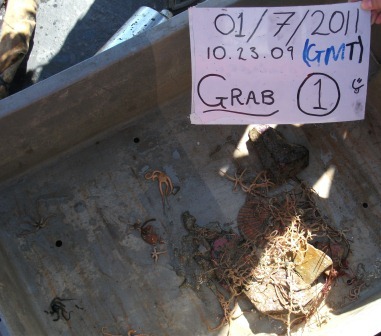
Before raising and lowering the grab over the side of the vessel the jaws were locked open. The grab was hoisted up and made adjacent to the vessel using the crane someone holding the grab to prevent it swinging. It was then lowered into the water and down to the seabed. As the grab hit the sea bed, lag in the chain disconnects the chain from the leaver leading to closure of the jaws as the grab is pulled up. The grab was steadied again as it was lowered onto the deck (inside a sampling tray) and a further two people were required to manually open the jaws and lift the device leaving the contents in the train for observation. (Left hand picture) The contents sample was photographed with an object (tape measure) to give an element of scale. Biological contents were observed, noted and removed before sediment sieving to prevent injury and desiccation. The remaining sediment was placed into a stack of sieves ranging in mesh sizes: 1cm, 1mm and 0.5mm ordered respectively from top to bottom. Water was poured over in a steady manner to aid grain separation into the separate sieve chambers. The sieves were separated from each other after sorting and the contents were photographed with an object for scale and analysed to give the percentage composition of each grain size relative to the total grab sample. The sieves and the sample tray were emptied overboard and rinsed with a water pump/bucket of water leaving them ready for the next sample. (Right hand picture) |
|
| Video Trawl | |
| The video trawl was lowered over the side of the ship and towed behind whilst we travelled at a speed of about 4 knots. The camera was lowered and raised as appropriate to view the seabed and what lay on it. The images were recorded to a DVD. |
|
|
|
|
|
|
|
|
The sidescan trace shows numerous rocky outcrops from 0.3 to 1.6m height. The area surrounding these rocks is mainly composed of maerl and coarse to very coarse sediment, as seen in figure 10. An unknown outcrop protrudes 0.8m from the seabed at 28850m Northings, 183317m Eastings to 28860m Northings, 183325m Eastings; although this outcrop was not identifiable, it was seen as noteworthy. Various scour regions were identified around the western end of the centre transect, along with anchor marks at 28800m Northings, 183260m Eastings. There is an area of coarse shales and fragmented rock spanning the Eastern end of transect 5, located between two rock outcrops, which would suggest break off from the larger rock formations. At 28570m Northings, 183265m Eastings, an approximately 25m long shipwreck was seen.
|
|
|
Figure 9 Results of sidescan track |

| Grab Site 1 | Grab Site 2 | |
| Time (GMT) | 10:23:01 | 10:40:02 |
| Depth (m) | 21.7 | 21.4 |
| Northings | 28982.9 | 28561.5 |
| Eastings | 183369 | 183372 |
| Latitude | 50 07 16.640N | 50 07 03.019N |
| Longitude | 005 01 54.934W | 005 01 53.922W |
| Benthic fauna present | Ophiuroids (Brittle stars) | Ophiuroids (Brittle stars) Tubiculous polychaetes |
Grab 1- This grab was taken along the most northern rock outcrop, which meant that there was a lack of finer sediment, this could perhaps be due to rocks blocking the grab jaws. Grabs are used as a way of ground truthing; however, because of the inability for the grab to fully close, a representative sample was unable to be extracted and sieved. Brittle stars were the most abundant fauna that was found, although different sessile fauna may have been attached to hard rock that was unable to be extracted with the grab.
 |
 |
| Figure 10.1 Contents of the first grab | Figure 10.2 Close up picture of the first grab |
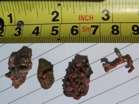
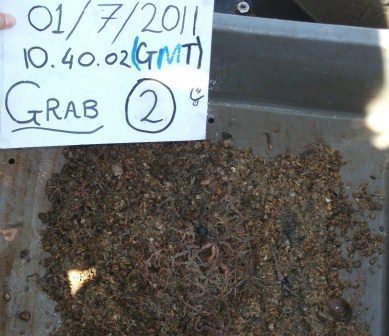
Grab 2- The jaws of this grab was not restricted by large rock, which meant that mid to coarse sediment was found in this area and therefore able to be sieved. After sieving, the largest percentage of material was in the 1cm-1mm size fraction. There were only 4/5 small rocks present in the grab sample that were larger than 1cm. Again there was a large population of brittle stars and different species of free and encrusting maerl. Tubiculous worms were found on large rocks, but due to the fact that these were unoccupied tubes, it is believed that the rock came from a rock outcrop. The sea bed at grab site two was composed of fragment of shell and maerl (both alive and dead). When sieved the sample separated in to three components: 7% in the 1cm fraction, 73% in the 1mm fraction and 20% in the 0.5mm fraction.
 |
 |
| Figure 11.1 Contents of the second grab | Figure 11.2 Close up contents of the second grab |

Following taking the grabs, a video trawl was used to produce photographic data of the sediment and biota of the seabed from grab site 2 back up to approximately grab site 1. The video images that could be seen were about 20m depth, roughly a metre off the seabed surface. Ophurioids were seen in abundance from the video footage, which confirms what was found from the grabs that were collected and analysed on deck. The sediment that was also collected from the grab samples and then sieved to determine the percentage of different grain sizes, correlated with the video recording. This means that when the veen grab and the video trawl are used in conjunction with one another, it is possible to fully appreciate the epifauna and the infauna on and within the benthos, respectively.
|
|
|
| Figure 12.1 Still image from the video trawl | Figure 12.2 Still images from the video trawl |
|
|
|
|
|
|
|
The majority of the surveyed area is occupied by maerl, both dead and alive. The reasons for this are sufficient light down to depths of 25m and also a moderate amount of water flow, preventing burial by sediments due to strong tides. The western coast of Falmouth Bay provides protection from powerful westerly storm systems, allowing fragile habitats, predominantly maerl habitats, to exist within the bay (Newton, 2011).
There were very few Bedforms that were picked up on the geophysical survey, perhaps due to the large grain size that is present, figure 10. However, the main factor as to why no bedforms are present is because of the calm climatic conditions that were found on the days leading up to the day of survey, preventing the formation of seabed ripples caused by high-energy wave action (Hall-Spencer and Atkinson, 1999).
Scour and anchor marks are present and easily evident on the sidescan track plot. This is undoubtedly from commercial vessels that frequently anchor in the surveyed area. This could have a potential impact on maerl beds and deep burrowing organisms because the anchor penetration is estimated to be about 25m depth. The mechanical interference of the anchor alters the benthic complexity and community structure of the seabed (Newton, 2011).
The southernmost area of the transects, around grab site 2, showed a large amount of fragmented shells, making up a high percentage of the composition of the sediment. This would suggested greater mechanical disturbance due to strong tides, currents and storms from the South-West that are particularly prevalent (Newton, 2011).

Extensive mearl beds were observed which was surprising as they are more commonly found around Saint Mawes Harbour and up Carrick roads. This could indicate that the mearl is spreading out into the bay, possibly carried on anchors from ships that first berthed in Carrick roads and then later moved out into the bay to avoid berthing costs. This is demonstrated by the anchor and scour marks on the transect. Large densities of Ophuiroids found in grab 1 and to a lesser extent in grab 2 convey low diversity, however due to a misleading grab sample this cannot be assumed. The large numbers of Ophuiroids are also confirmed by the video trawl which was taken between garb sites 1 and 2. Large numbers could be explained by a strong enough flow for productive suspension feeding without too greater currents to continually re surface the seabed in the form of sand ripples. Hard substrate provided by the rocky outcrops could also provide leverage against tidal action.
|
|
|
|
|
|
|
|
|
To determine the chemical, biological and physical parameters and interactions within the Fal estuarine environment and its main sources
To link the physical and chemical properties to freshwater inputs and mixing which in turn affect the biology
To observe whether nutrients such as silicon are affected by mixing and whether this is the only factor.
On the Tuesday 5th July 2011, the plan for the day was to start at Black Rock, at the mouth of the estuary, sample there and then head into the Fal estuary and up the Carrick Roads. This was to find out the changes in water from saline to more freshwater composition. The Carrick Roads then merged into the River Fal, where a more freshwater influence was predicted. Station 1 is to be measured at high water, which is at 0757 GMT, expecting a low flow rate from the transect data as it is on slack tide. From this point, the following stations will be measured on an ebbing tide, hoping to reach the final station (station 7) before low water, 1417GMT. At each station a CTD profile is to be carried out recording salinity, temperature, transmission and fluorescence changes against depth. In addition to this, at certain stations an ADCP transect will be recorded to gauge altering flow rates up the estuary. At 3 stations, Black Rock, station 5 and station 7 respectively, a plankton net will be deployed for 5 minutes, to collect zooplankton samples. From this it is possible to compare the biota dynamics throughout the estuary. Light irradiance will be measured at every station with an irradiance metre to calibrate the CTD transmission data.
 |
 |
| Figure 13.1 Image of ADCP tracks and CTD stations up the Fal estuary | Figure 13.2 Close up image of ADCP tracks and CTD stations |
|
Estuarine-5.7.11 |
|||||
|
Station Number |
Time (GMT) |
Latitude (N) |
Longitude (W) |
Water Depth (m) |
Weather (cloud cover) |
|
1 |
0815 |
50°08.665 |
005°01.463 |
35.0 |
7/8, stratus cloud |
|
2 |
0913 |
50°09.601 |
005°02.184 |
35.8 |
8/8, stratus cloud, drizzle |
|
3 |
1013 |
50°10.838 |
005°01.703 |
30.0 |
3/8, cumulus & cirrus cloud |
|
4 |
1115 |
50°11.522 |
005°03.550 |
|
5/8, cumulus & stratocumulus cloud |
|
5 |
1156 |
50°12.443 |
005°02.018 |
14.6 |
6/8 |
|
6 |
1237 |
50°13.501 |
005°00.955 |
13 |
4/8 |
|
7 |
1320 |
50°14.410 |
005°00.880 |
3.4 |
7/8, stratocumulus cloud |
|
|
|
|
|
|
|

A zooplankton net with a mesh size of 210µm was deployed over the stern of RV Bill Conway. The net was towed horizontally at a constant depth, directly behind the vessel for a period of 5 minutes. A flow metre was attached to the mouth of the net in order to record the rate at which the water and therefore biology was entering the net.
Light irradiance was measured with an instrument that recorded the light levels within the water column and the atmosphere. The measurements were taken in air due to the fact that there is perfect transmission, no absorption or attenuation, and therefore these values can be compared to the values from the water. Two sensors were used, one for the air and one for the water column. Before the water sensor was lowered into the water both sensors were calibrated against each other. The water sensor was lowered into the surface water and a measurement was recorded, before being lowered metre by metre, with measurements taken at each point. This occurred at all stations except for station 1.
The RV Bill Conway is set up with a continuous water pumping system, which was used to extract surface water at a 1.2m depth. Samples were taken from the pumping system and a T/S probe was used to calibrate the salinity measurements with the CTD values.
A rosette sampler, with a CTD and 5 Niskin bottles, and the secchi disc were deployed as described in the offshore procedure. All wet lab methods were also consistent with those described in offshore procedure.
The shore lab procedures for silicon, phosphate, dissolved oxygen, chlorophyll and phytoplankton and zooplankton analyses are also all the same as those conducted in the offshore shore lab. See offshore methods for details.
|
|
|
|
|
|
|
| Figure 14.1 Station 1 | Figure 14.2 Station 2 |
|
|
|
|
Station 1 has a chlorophyll minimum of 6µg/L at 23.5m and a maximum of 11µg/L at 18m. It is relatively constant in the water column despite spikes. Salinity is constant throughout the water column at 35.5. The temperature decreases with depth from a surface maximum of 15.4°C to a minimum at 28m of 15.1°C. Silicon declines with depth then increases. Phosphate follows the same trend as silicon. Dissolved oxygen declines with depth from a maximum at the surface of 275µmol/L declines to 15m where the decrease becomes less sharp to a minimum of 260µmol/L. Transmission is constant throughout the water column at 4.43v. |
The chlorophyll is constant throughout the water column at 7.5µg/L, with a peak at 11m, however, this could be a spike. The entire profile shows significant spiking throughout the water column. Salinity is constant throughout the water column at 35.5PSU. Temperature is relatively constant with a small decrease of 0.1°C at 11metres. Transmission is constant throughout the water column at 4.42v. Silicon is 1.2µg/L at the surface decreasing to 1µmol/L at 9m then remains constant. Phosphate is constant throughout the water column at 0.02µmol/L. Dissolved oxygen increases from the surface to 9m with the minimum at the surface being 249µmol/L. It is then constant from 9 to 20 metres, and from 20 to 30 metres there is further increase to a maximum value of 269µmol/L. |
| Figure 14.3 Station 3 | Figure 14.4 Station 4 |
|
|
|
|
Chlorophyll increases from the surface to 5m where it peaks at 10µg/L, at 7 metres it begins to decline to 6µg/L at 10m, then remains constant. Transmission increases from 4.4v at 3m to 4.45v at 8m, then is constant at 4.45v. For salinity, only noise is visible due to a CTD error. Temperature is constant in the water column at 15.5oC. Silicon decreases to 0.9µmol/L at 4.5m, then increases up to 8m, where it remains constant. Dissolved oxygen decreases from 260µmol/L at the surface to 255µmol/L at 5m, peaks at 6 metres at 290µmol/L before decreasing to 262µmol/L at 20m. Phosphate increases from the surface to 5m where it reaches 0.025µmol/L, then decreases to 0.02µmol/L at 8m, remaining constant in the water column. |
Chlorophyll is 7.5µg/L at the surface, increasing steadily to 10µg/L at 5m depth. Transmission is constant at 4.28v with a spike at 1m depth. Salinity is constant at 34.7 as is temperature at 16.5°C throughout the water column. Due to the fact that water samples were collected at 1 depth, trends for silicon, phosphate and dissolved oxygen cannot be observed, only the values at 5m can be observed. |
| Figure 14.5 Station 5 | Figure 14.6 Station 6 |
|
|
|
|
Chlorophyll increases from 7.5µg/L at the surface to 10µg/L at 5 metres, then becomes constant for the rest. Transmission is constant at 4.2v. Salinity is constant at 35 as is temperature at 16.6°C throughout the water column. Silicon is constant at 2.1µmol/L and phosphate is also constant at 0.04µmol/L. A trend for dissolved oxygen cannot be observed as only 1 bottle was collected at 5m. This was because we only had a limited number of dissolved oxygen bottle. |
Chlorophyll increases from the surface where it is 10µg/L to 2 metres where it is 19µg/L, then it is constant in the water column to 8 metres, a spike is present at depth. Transmission steadily increases from 3.8v at the surface to 3.9v at 28 metres. Salinity follows transmission, but is higher, increasing from 32.7 at the surface to 33.5 at depth. Temperature is 18°C at the surface and increases with depth to 17.6°C. Silicon decreases from 4.9µmol/L at the surface to 3.6µmol/L at depth. Phosphate is constant at 3.9µmol/L. |
| Station 7 did not have a CTD profile taken due to the shallow waters occurring due to being far up the estuary as well as it being very close to low tide. | |
Salinity Calibrations
The sailinities from these CTD profiles can only be used for trends, not for values due to the fact that the calibrations were inaccurate. The graph below shows the salinities which were recorded by different groups at roughly the same position close to Black Rock at the mouth of the Fal estuary. It clearly shows that the salinities recorded had very different values ranging from 35.0psu to 35.6psu.
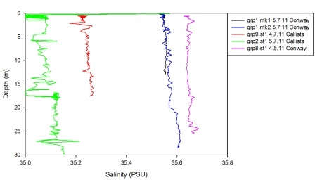 |
| Figure 15 Salinity calibrations between different groups results at Black Rock |
The salinities collected on the 5th July 2011 in the Fal estuary showed some inconsistencies when analysed. For example, Station 3 exhibits salinity values of greater than 36 PSU with extensive spiking as the CTD progressed down through the water column. As this station is located further up the estuary it is highly irregular to find salinity values so much higher than those at the mouth. This implies that these results are inaccurate or there could have been problems with the sampling equipment and calibrations.
The CTD salinity values were compared between the RV Bill Conway and the RV Callista from the stations closest to Black Rock situated at the mouth of the estuary as both vessels sampled this location. At the time of data collection the CTD from the Callista experienced technical trouble and thus the station at Black Rock was not sampled until about 1500GMT. Whilst it is still possible to compare these salinities it would require knowledge of the salinity variation at Black Rock over 6 hours. Data collected on the 4th July 2011 by both Callista and Conway was able to be sampled at Black Rock at about the same time and is therefore directly comparable.
Both vessels sampled the first 15m of the water column and the mean average salinity found for data from each vessel. Data from the Callista showed the average salinity to be 35.2 whilst data from Conway was higher at 35.6. This implies the salinity reading from the Callista was correct and no variance in time or space was evident between the samples.
The difference between the values can therefore be used to correct the Conway CTD salinities collected by subtracting 0.40685 PSU from each of the salinity values. However, the time at which the change in the CTD salinity sensor occurred is unknown. If the change occurred before the samples were taken on the 5th July this difference can be corrected for throughout the dataset. However it maybe the case that some of the first stations sampled may give accurate salinity values whilst those sampled later in the day needed to be corrected. For this reason it is not possible correct the dataset collected on the 5th July even though some stations exhibited unusual trends.
Salinity values provided in the CTD profiles may not be accurate and therefore only the trends exhibited and not qualitative values of individual points will be used. Temperature values can also be used to help explain the changes in the salinity trends and where possible the CTD readings will be compared to the YSI probe measurements. Unfortunately it is not possible to provide an accurate calibration between the YSI measurements and CTD data as the T/S probe was used on a small number of the total samples.
Optics
Using the transmissometer data from the CTD it is possible to analyse the transmission of light within water. Using this data the beam attenuation coefficient can be calculated. Initially, calibration of the transmissometer is required. Whilst on the back deck of the RV Bill Conway a light and dark reading was taken-the light in full sunlight and the dark reading by shielding the sensor on the instrument preventing light getting across. The CTD dark reading was 0.000 ±0.01 V whilst the light reading was 4.510 ±0.03 V. As the dark reading equals 0, further adjustment of the transmissometer data for the CTD profile was not required. The Beer-Lambert Law is used to calculate the attenuation of light in water:
|
|
ocean=transmissometer reading at depth
light air=surface light reading (4.51 V) d=aperture size=50 mm=0.005 m c=attenuation coefficient |
Attenuation is made up of two components; the attenuation due to water and the attenuation due to particles:
|
|
c=attenuation cw=attenuation due to water cp=attenuation due to particles. |
The transmissometer operates on a wave length of 650nm. At this wave length the attenuation for pure water=0.350 m-1 (Knauss, 2005). Particles in the river water include nutrients and organic matter, therefore can be used in comparison with the chlorophyll data to provide evidence of high phytoplankton areas. The attenuation of light due to particles in the water is:
![]()
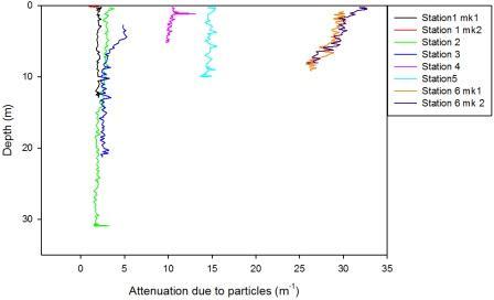 |
|||||||
| Figure 16 Attenuation of light due
to particles in the water
This data can be further extended by using the diffuse irradiance attenuation coefficient. This is calculated using the irradiance meter data and the Beer-Lambert Law.
Plotting the irradiance meter data in this ln(Iz)/ln(I0) format, the gradient of the linear treadline between the points equals the diffuse irradiance attenuation coefficient. Using the c value calculated earlier this kd can be used to link a number of different light measurements undertaken in the estuary.
By plotting the secchi depth reading against 1/kd+c (where secchi is on the y axis) it is possible to calculate this constant. The gradient of the linear treadline between the points will be the value of this m. For the data collected within the Fal estuary for this date the m value is 9.5. This can now be compared to other m values within the literature, such as Kirk’s book and Gordon’s paper. Kd can be used to classify water classes (Jerlov, 1976) and is a critical parameter for accurate estimation of the light intensity at depth (Simpson & Dickey, 1981). Using these equations the data from the secchi disk, irradiance meter and CTD transmissometer can all be linked, and when combined can be used to describe the optical water properties of the estuary. This can be used to imply the amount of particles in the water-and when combined with the CTD Fluorimeter reading can support data for chlorophyll abundance-a high chlorophyll reading would result in a decrease in the amount of light penetrating the water column as it is all being blocked out by the photosynthetic organisms. In addition the data can be combined with ADCP data to look at turbulence, as this will also decrease the distance light is able to penetrate the water. |

|
|
Copepoda 44% Echinoderm larvae 30% Gastropod larvae 9% |
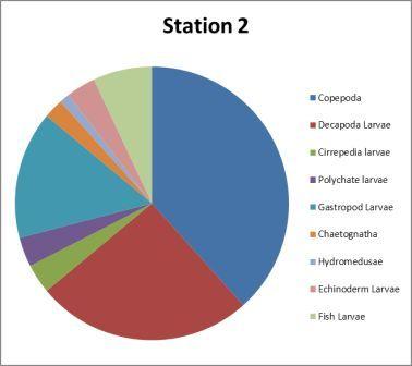 |
Copepod 38%
Decapoda larvae 26% Gastropod larvae 15%
|
| Figure 17.1 Station 1 - Mouth of estuary | Figure 17.2 Station 5 - Middle of estuary | ||
|
|
Copepoda (54%) Gastropod larvae (14%)
Mysidacea (14%)
|
||
|
Figure 17.3 Station 7 - Top of estuary |
|||
NB: Information about the major zooplankton types can be found in the offshore zooplankton section.
| Cells per m^3 | Station 1 | Station 2 | Station 3 | Station 5 | Station 7 |
| Diatoms | |||||
| Chaetocerotaceae | 60000000 | 40000000 | 260000000 | 240000000 | 0 |
| Rhizosoleniceae | 90000000 | 30000000 | 40000000 | 170000000 | 50000000 |
| Thalassiosiraceae | 290000000 | 370000000 | 110000000 | 160000000 | 300000000 |
| Coscinodiscus (Family:Coscinodiscaceae) | 70000000 | 110000000 | 270000000 | 0 | |
| Skeletonema (Family:Skeletonemaceae) | 60000000 | 50000000 | 70000000 | 1390000000 | 61925000000 |
| Bacillariaceae | 100000000 | 80000000 | 260000000 | 1225000000 | |
| Hemiaulaceae | 0 | ||||
| Diatoms | 80000000 | 110000000 | 0 | ||
| Dinoflagellates | |||||
| Prorocentraceae | 40000000 | 0 | |||
| Armoured Dinoflagellate | 40000000 | 30000000 | 0 | ||
| Dinophysiaceae | 50000000 | 1000000 | 0 | ||
| Naked Dinoflagellate (Pyrophocus) | 30000000 | 0 |
The phytoplankton samples taken from the niskin bottle samples showed a reduced diversity compared to that seen in the offshore samples. The thalassiosiraceae, rhizosoleniaceae and skeletonemaceae families were present in high densities at all stations where phytoplankton sampling took place; with chaetocerotaceae also being in high abundance but absent at station 7. At station 1 thalassiosiraceae were the dominant family with 2.9x10⁸ cells per m3; this family was also showed the highest abundance at station 2 with 3.7x10⁸ cells per m3, with just 8x10⁷ cells per m3 of unidentifiable centric diatoms at the same station. Thalassiosiraceae seems to show highest density at station 2 near the mouth of the estuary and further up the river at station 7. Bacillariaceae was also in high density at station 1 with 1x10⁸ cells per m3; this family also showed quite high numbers in stations 5, 2.6x10⁸ cells per m3, and 7, 1.23x10⁹ cells per m3. The most abundant family at station 3 was chaetocerotaceae , 2.6x10⁸ cells per m3; this station also included thalassiosiraceae, coscinodiscaceae and unidentified diatoms all at a density of 1.1x10⁸ cells per m3. At stations 5 and 7 the family skeletonemaceae was dominating, with a density of 1.39x10⁹ cells per m3 at station 5 and 6.19x10¹⁰ cells per m3. Coscinodiscaceae, bacillariaceae and chaetocerotaceae were all also in high densities, 2.7 2.6 and 2.4 x10⁸ cells per m3 respectively, in station 5. Dinoflagellates were more consistent in the estuarine samples than in the offshore samples; there were many samples from offshore that had no dinoflagellates identified, whereas, in the estuarine samples, stations 1, 2, 3 and 5 all contain dinoflagellates. The numbers of the dinoflagellates seem to be decreasing further up the estuary; for instance, there were 5x10⁷ cells per m3 of the family dinophysiaceae at station 1 which decreased to only 1x10⁶ cells per m3.

| Figure 18.1 Station 1 | Figure 18.2 Station 2 |
|
|
|
|
There is a low, consistent amount of backscatter across the entire transect at around 68dB. The flow direction is in a southward direction for the western third of the transect (the right side of the image). After this point the top half of the water column has no coherent direction, with flows in every direction. The bottom half of the water column in the eastern two-thirds of the transect shows a general northerly trend. The average velocity is 0.31 ms-1. |
There is a low and consistent backscatter across the entire transect at around 67dB. The flow direction begins in a southerly direction in the West of the transect (the right side of the graph) and gradually changes direction throughout the transect, becoming easterly at the centre and eventually developing into a northerly flow in the eastern side of the transect. The average velocity is 0.43 ms-1. |
| Figure 18.3 Station 3 | Figure 18.4 Station 4 |
|
|
|
|
There is a low and consistent backscatter across the entire transect at around 63dB. The flow direction is southerly for the entire transect save for the central channel, where it becomes easterly briefly. The average velocity is 0.24 ms-1. |
There is low and consistent backscatter across the transect at around 68dB. The majority of currents across the transect flow in a southerly direction, changing to an easterly direction in the eastmost quarter. The average velocity is 0.18 ms-1. |
| Figure 18.5 Station 5 | Figure 18.6 Station 6 |
|
|
|
|
There is low and consistent backscatter across the transect at around 75dB. The current flows almost uniformly in a north-western direction, with the only difference in the southmost quarter of the transect, where the currents flow in different directions throughout the water column. The average velocity is 0.26 ms-1. |
There is low and consistent backscatter across the transect at around 80dB. The current flows mostly in a southern direction, with surface currents being more variable. The currents in the top 1.5m are northerly in the western end of the transect, then southerly for most of the central transect, then easterly for a brief period, then back to southerly and finishing in the eastern end of the transect flowing once more in a northerly direction. The average velocity is 0.29 ms-1. |
| Figure 18.7 Station 7 | |
|
|
There is low and consistent backscatter across the transect at around 80dB. Current direction is very variable throughout this transect, though the current flows mostly in a southerly or easterly direction. The majority of the easterly flowing currents are in the centre of the transect, while the eastern and western edges are mostly southerly flowing currents. There are occasional northerly currents scattered throughout the width of the transect at varying depths. The average velocity is 0.09 ms-1.
|
| Figure 18.8 Richarson Number for Station 6 | |
|
|
Station 6 is the only station where shear was observed between 2 different water masses and because a front was clearly observed at the water surface. There are 2 large stable layers between 2m and 4m depth and between 5 and 7m depth. These 2 layers are separated by a small layer of instability where mixing was occurring between the 2 stable layers. |

Mixing diagrams for both phosphate and silicate generally show non-conservative
behaviour however they differ in addition and removal respectively. Phosphate is
strongly added to the Fal Estuary especially below salinities of 35, with the
exception being at a salinity of 11.7. Phosphate does however show some removal
at very high salinities due to phytoplankton growth in the mouth of the estuary
counter-acting addition from agricultural and sewage effluent sources. Silicate
shows removal especially below salinities of 34, this is unquestionably due to
removal by numerous diatoms utilising silicate particularly
Skeletonema and Thalassiosiraceae. ~
The majority of the samples were collected aboard the R.V Bill Conway
on 05/07/2011 and indeed the seawater endmember was determined on this cruise.
However the riverine endmembers were collaborated from a couple of freshwater
tributaries of the River Truro namely the River Allen and River Kenwyn and a few
intermediate salinity samples were collected from these rivers around the Truro
region.
Salinities were on the whole measured using a CTD system however this was not
available for 3 samples collected from the surface and some error may be
applicable for salinity measurements in these samples.
| Figure 19.1 Estuarine mixing diagram for Phosphate in the Fal estuary | |
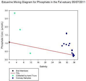 |
It is evident from the estuarine mixing diagram for phosphate that there
is a strong addition of phosphate to waters with salinities less than
35, with the exception being at a salinity of 11.7 where there is in
fact evidence of removal of phosphate. The trend throughout however is
non-conservative behaviour with the exception at very high salinities
greater than 35 where perhaps phytoplankton growth removes phosphate
that has been added to the water column. The addition of phosphate within the Fal estuary, especially the upper reaches where salinities are lower, can be attributed primarily to diffuse sources particularly from run off (or leaching) of the surrounding land catchment area either directly or through groundwater flow. This is exacerbated by the fact that the freshwater catchment of the Fal lies in an extensive farming area for both arable and diary methods many of which practice fertiliser intensive agriculture (Langston, 2003). Also further increasing phosphate addition into the Fal is because the underlying bedrock of the catchment area is impermeable rock, thus along with high annual rainfall totals the annual runoff is 719mm/yr (Fraser et al, 2000) contributing vast concentrations of phosphate into the Fal. This accounts for the strong addition of phosphate in regions of salinity between 29 and 35. The samples collected by hand with salinities of 3 and 6 show extremely strong non-conservative behaviour with concentrations 1.7µmol/L and 0.7µmol/L greater than the TDL respectively. This is undoubtedly a result of addition from sewage treatment works point source at Malpas and Truro (Langston, 2003). This often peaks during the summer when rainfall levels are generally low, mixing is at a minimum and sewage levels increase coinciding with a peak in visitor numbers to the South West. These large inputs of phosphate into the estuary resulted in the upper Fal being classified as a potentially sensitive area (eutrophic) in 1997. This followed a period of successive years (1995 and 1996) when toxic algal blooms of Alexandrium affected the upper Fal estuary and Truro River, two regions which show strong addition of phosphate in the estuarine mixing diagram for phosphate. This coinciding with fluctuations of dissolved oxygen and chlorophyll concentrations leads to eutrophication of the upper Fal estuary. At a salinity of 11.7, bucking the general trend of addition there is indeed removal of phosphate. One potential reason for this observation is that phosphate can be readily absorbed onto particulates (Langston, 2003). Therefore in turbid waters where there is suspension of particulates there may be significant removal of phosphate to the sediments as experienced at a salinity of 11.7. This could be caused by an interface between fresh and saline waters in the River Fal which re-suspends sediments absorbing phosphate. However there could also be an outfall of low concentration phosphate near the lock gates where the sample was taken. |
| Figure 19.2 Estuarine mixing diagram for silicon in the Fal estuary | |
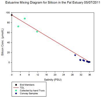 |
Silicate is added to the Fal estuary through weathering of silicate
minerals in the surrounding catchment area. Therefore silicate
concentrations are far higher in freshwater than saline. In the silicate
mixing diagram the samples collected do not follow the TDL therefore
their concentrations are not determined by simple mixing. There is some
degree of removal present. |

| Figure 20 Discharge flow rates for the Fal Estuary | |
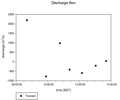 |
The first three data points lack in accuracy due to the absence of a large portion of data as the channel was to deep for the ADCP to reach the seabed. The first station was surveyed on slack tide showing high (2191m3/s) north bound flow in the measured available data. There is a large difference in transect 2 relative to transect 1 where the average flow (796m3/s) is south bound however a large chunk of the data is also missing in the deepest area of the transect thus the average flow magnitude and direction is not reliable. The same can be said for transect 3 with the ADCP unable to measure the deepest point in the transect therefore heavily skewing the averaged flow. This could explain the large magnitude of flow (984m3/s) northbound where in truth south bound flow through the unmeasured area could cancel out large figure. The remaining transects all show negative values (-412.1, -590, -203.7m 3/s respectively) with the exception of final transect which was measured close to slack tide (14:17 GMT). The mean flow for this transect (40m3/s) is close to 0m3/s as expected for slack tide. The negative flows correlate to measuring against an ebbing tide with the flow heading south out of the estuary. These transects appear more accurate as all of the area was measured by the ADCP creating a true representation of the average flow rate at that point and time within the estuary.
|
|
|
|
|
|
|
|
Station 1- Black Rock- Between Shag Rock and Pendennis Point
A gradual thermocline of 0.3˚C, can be observed in the upper 20m of the water column. This can be attributed to solar radiation and low mixing. The weak gradient of the thermocline may show that was being broken down, whilst on station we observed large swell, which could have caused this breakdown. At 22m there is strong evidence of a denser water mass compared with the surface well-mixed layer, caused by cooler temperatures and higher salinity. More oxygen is diffused into the water column because of wind mixing, demonstrated by slight variations in the upper temperature profile.
Station 2 - Between St Mawes Castle and Trefusis Point
A thermocline can be seen at 10m, which may indicate a different water mass at depth with a slightly higher salinity than the one above it. There are higher chlorophyll concentrations in the upper mixed layer, which may be correlated to the higher transmission in surface waters indicating a large number of particles. Dissolved oxygen however shows an unusual trend in being lower in concentration in the surface layers than those experienced at depth. One possible reason for this is that the water at in the bottom layers is colder than that in the surface layers giving it a higher solubility factor.
Station 3- Between Messack Point and Penarrow Point
Again, two separate water masses can be seen. The upper one can be defined by high chlorophyll and low transmission indicating the presence of large numbers of phytoplankton. This is also supported by the slightly higher surface temperatures. A reduction of silicon is evident from the surface waters to 4m, which also correlates to the increase in chlorophyll measurements and therefore could be due to diatom uptake. There appears to be an anomaly in the dissolved oxygen concentration at a depth of 8m showing a value of 289µmol/L. This is far greater than any experienced throughout the estuarine survey and could have been caused by human error in the laboratory method.
Station 4- Between Restronguet Point and the edge of land
There is evidence of a thermocline
present at a depth of 2m, coinciding with a slight halocline at the same depth.
This suggests a freshwater layer overlying a denser, cooler, more saline layer
beneath. This can be expected at station 4 which was at the mouth of Restrongue
Creek where freshwater flows out into Carrick Roads.
Station 5- Between Turnaware point and Bottom of South Wood
Station 5, like that of station 4 shows a slight thermocline at a depth of 2m
suggesting a surface mixed layer, which is slightly depleted in silicon
concentration when compared to a depth of 10m. When comparing this to the mixing
diagram for silicate there is indeed removal at this station attributing to
utilisation by diatoms in the surface layer.
Station 6- Between 2 edges of land by where Truro River flows into the Fal
Where station 6 was sampled there was clear evidence of a visible front as
surfactants on the surface converged, caused by freshwater input from the River
Fal meeting saline tidal waters from the Fal estuary. The CTD profile at station
6 shows 3 distinct layers, the first is a surface, warm, fresh layer with low
turbidity and chlorophyll. This layer is therefore likely to be a buoyant
freshwater water type inputted from the River Fal, perhaps following heavy rain
that was experienced overnight of the 05/07/2011. An intermediate water layer
found between a depth of 1.2m to 5.5m is clearly evident, which is more saline
than the upper 1.5m surface layer, with a temperature some 0.3°C cooler. This is
likely to arise through the simple mixing between freshwater in the surface
layers and dense, cool, saline waters below a depth of 5.5m. Chlorophyll shows a
rapid increase from the surface layer to the mixed intermediate layer beneath.
Indeed this chlorophyll concentration of 18µg/L is twice as high as anywhere
experienced throughout the estuarine survey; this can be attributed to a very
strong nutrient input of both phosphate and silicon shown by high concentrations
in the surface layers of 0.7µmol/M and 4.7µmol/L respectively. The water mass
below 5.5m shows a gradient in both temperature and salinity which creates a
cooler, more saline water that is denser than that in the surface layers.
Chlorophyll appears to stay constant in this dense water layer however turbidity
increases which could be caused by suspended sediment disturbed by an ebbing
tide. Finally there is an apparent decrease in silicate compared to the high
concentrations shown in the surface layers. This, when comparing to the mixing
diagram for silicate at salinities of 33.5 shows removal of silicate as diatoms
utilise this for their frustules.
Phytoplankton Interpretation
As was seen in the coastal phytoplankton counts, large numbers of diatoms co-exist with dinoflagellates; this is possible because the two groups utilise contrasting tidal mixing properties of the estuary (Lauria et al, 1999). There seemed to be slightly fewer dinoflagellate specimens further up the estuary, this suggests that there are fewer species of dinoflagellates can withstand the variable environment seen in estuaries.
The density of skeletonema was highest at that station furthest up the estuary where the salinity of the water reached around 30psu. Some species of skeletonema are known to grow well between salinities of 10 and 35; others such as S. costatum and S. subsalsum can even grow between salinities of 0 and 35 (Balzano et al, 2011). Bacillariaceae are also in high densities at station 7; this is perhaps due to the absence of halophilic diatoms (Frankova-Kozakova et al, 2007).
Chaetocerotaceae show a high diversity in stations 3 and 5 but are absent in station 7; this may have been due to increased freshwater input at station 7 or increased competition from the increased skeletonema species. Competition may have also come from thalassiosira; as there is a higher density of this genus at station 7 than were found at station 3 or 5 where chaetocerotaceae bloomed. There only seemed to be lower densities of rhizosoleniceae, thalassiosiraceae, skeletonema and bacillariaceae at station 7 which could indicate a wider salinity tolerance. Brand (1984) found that a few species of the genus Chaetoceros could grow well down to salinities of 15 and up to an optimum of 33 to 45. Brand also found that estuarine species of Thalassiosira were able to grow in a freshwater medium and that Skeletonema had a broad salinity range between 15 and 45.
Conclusion
As is to be expected from an estuary, there are two distinct water masses at each station, showing the interaction of fresh riverine input with saline oceanic water. The only exception is at Station 6, where there are three separate water masses . Two of these are intersecting rivers, and the third is the incoming saline oceanic water.

|
|
|
|
Offshore
Baier, C. T. and Purcell, J. E. 1997, ‘Trophic interactions of chaetognaths, larval fish and zooplankton in the South Atlantic Bight’, Marine Ecology Progress Series, 146, 43-53
Bentley, D. Hart, V. Guary, J. Statham, P. 1999, Dissolved nutrient distributions in the Central English Channel, Continental Shelf Research 19, pg 2083-2099
Bryan, J. R., Riley, J. P. and Williams, P. J. LeB., 1976, ‘A Winkler procedure for making precise measurements of oxygen concentration for productivity and related studies’, Journal of Experimental Marine Biology and Ecology, 21, 191-197
Bustillos-Guzmán, J. et al., (2000). Pigment signatures associated with an anoxic coastal zone: Bahia Concepcion, Gulf of California. Journal of Experimental Marine Biology
Digby, P. S. B. 1950, ‘The biology of the small planktonic copepods of Plymouth’, Jour.Mar. Biol. Assoc., vol XXIX, 393-426
Guillard, R. R. L. and Kilham, P., 1977, ‘The ecology of marine planktonic diatoms’, in Werner, D. (ed), The Biology of Diatoms, Blackwell Scientific Publications, Berkeley and Los Angeles, California, 372-469
Harris, R., 2010, ‘The L4 time series: the first 20 years’, Journal of plankton research, 32, 5, 577-583
Holligan, P. M. and Harbour, D. S., 1977, ‘The vertical distribution and succession of phytoplankton in the western English channel in 1975 and 1976’, Journal of the marine biological association of the United Kingdom, 57, 1075-1093
Hoch, T. & Garreau, P. 1998, Phytoplankton dynamics in the English Channel: a simplified three-dimensional approach, Journal of Marine Systems, Vol. 16, pg 133-150
Jones, K. J. and Gowen, R. J., 1990, ‘Influence of Stratification and Irradiance Regime on Summer Phytoplankton Composition in Coastal and Shelf Seas of the British Isles’, Estuarine, Coastal and Shelf Science, 30, 557-567
Kiorboe, T. 1998, ‘Population regulation and role of mesozooplankton in shaping marine pelagic food webs’, Hydrobiologia, 363, 13-27
Knauss, J. A., 2005, Introduction to Physical Oceanography, 2nd ed. Cornell University, Waveland Press
Maddock, L., Boalch, G. T. and Harbour, S., 1981, ‘Populations of phytoplankton in the western English Channel between 1964 and 1974’, Journal of the marine biological association of the United Kingdom, 565-583
Miller, C. B., 2004, Biological Oceanography, Blackwell Publishing, Oxford, UK.
Parsons T. R. Maita Y. and Lalli C. (1984) “ A manual of chemical and biological methods for seawater analysis” 173 p. Pergamon
Pepper, I. L. and Gerba, C.P. (2004). Environmental mircobiology: an environmental manual. 2nd ed. London: Academic Press. 2009.
Sharples, J., Moore, M.C., Rippeth, T.P., Holligan, P.M., Hydes, D.J., Fisher, N.R., and Simpson, J. H., 2001. “Phytoplankton Distribution and Survival in the Thermocline”, American Society of Limnology and Oceanography, 46, 3, 486-496.
Strzepek, R. F. and Price, N. M., 2000, ‘Influence of irradiance and temperature on the iron content of the marine diatom Thalassiosira weissflogii (Bacillariophyceae)’, Marine Ecology Progress Series, 206, 107-117
Takahasi, D. and Ikeda, T. 2006, ‘Abundance, vertical distribution and life cycles patterns of the hydromedusa Aglantha digitale in the Oyashio region, western subarctic Pacific’, Plankton Benthos Research, 1, 2, 91-96
Widdicombe, C. Eloire, D. Harbour, D. Harris, R. & Somerfield, P. 2010, Long-term phytoplankton community dynamics in the western English Channel, Journal of Phytoplankton Research, Vol. 32, Issue 5, pg 634-655
Diatom Lauderia annulata Cleve 1873, [Online], 2010. Available: http://www.sahfos.ac.uk/taxonomy/phytoplankton/diatoms/lauderia-annulata-.aspx [accessed: 2011, July 6th]
Taxonomy – Phytoplankton, [Online], 2010. Available: http://www.sahfos.ac.uk/taxonomy/phytoplankton.aspx [accessed 2011, July 6th]
Geophysics References
Sidescan Picture - Able, K.W. et.al, 1987, ‘Sidescan-Sonar as a tool for detection of demersal fish habitats’, Fishing Bulletin, vol. 85, no. 4, 725-736.
Birkett, D.A., Maggs, C. and Dring, M.J., 1998, ‘Maerl (Volume V), An overview of dynamic and sensitivity characteristics for conservation management of marine SACs’, Scottish Association for Marine Science, 116pp.
Bosence, D. and Wilson, J., 2003, ‘Maerl growth, carbonate production rates and accumulation rates in the northeast Atlantic’, Aquatic Conservation: Marine and Freshwater Ecosystems, 13, 1, 21-31
Buchanan J.B, 1964. ‘A comparative study of some features of the biology of Amphiura filiformis and Amphiura chiajei [Ophiuroidea] considered in relation to their distribution’. Journal of the Marine Biological association of the United kingdom. 44 (03)
Deeble, M., and Stone, V., 1985, ‘A Port that could threaten marine life in England’s Fal Estuary’, Oryx, 19, 2, 74-78.
George J. D, Hartmann-Schroder G, 1985.’Polychaetes:British Amphinomida, Spintherida & Eunrcida.’ Synopse of the British fauna. 32:221
Hall-Spencer J. M, Atkinson R. J. A, 1999. ‘Upogebia deltatura (Crustacea:Thalassindea) in Clyde sea mearl beds, Scotland’. Journal of Marine Biology. association UK. 79:871- 880
Hiscock, K., Sewell, J., and Oakley, J., 2005, ‘Marine Health Check, A report to gauge the health of the UK’s sea-life’, Godalming, WWF-UK.
Johnsen S & Kier W 1999. ‘Shade seeking behaviour under polarized light of the brittle star Ophioderma brevispinium (Echinodermata:Ophiuroidea)’. Journal of Marine Biological association of the United kingdom. 77:761-763
Newton J, 2010/2011. Impacts of commercial anchoring on mearl beds in Falmouth bay. Avaliable: http.//www.falmouthport.co.uk/commercial/html/documents/AnchoringStudyJoeNewton.p df [accessed] 04/07/2011.
Warner G. F, 1971. ‘On the ecology of a dense bed of brittle-star Ophiothrix fragilis’. Journal of the Marine Biological association of the United kingdom. 55:199-210
Estuarine
Balzano, S., Sarno, D. and Kooistra, W. H. C. F., 2011, ‘Effects of salinity of the growth rate and morphology of ten Skeletonema strains’, Journal of Plankton Research, 33 (6), 937-945
Brand, L. E., 1984, ‘The Salinity Tolerance of Forty-Six Marine Phytoplankton Isolates’, Estuarine, Coastal and Shelf Science, 18, 543-556
Frankova-Kozakova, M., Marvan, P. and Geris, R., 2007, ‘Halophilous diatoms in Czech running waters: Pleurosira laevis and Bacillaria paxillifera’, Kusber, W. H. and Jahn, R. (eds), Proceedings of the 1st Central European Diatom Meeting 2007, 39-44
Fraser, A. I. Butterfield, D. Uncles. R, Johnes, P. And Harrod, T. R., 2000. ‘Fal and Helford Special areas of conservation (cSAC) and the Tamar estuaries complex cSAC/special protection area (pSPA): Estimation of diffuse and point-source nutrient inputs’. SSLRC report to the EA. 89pp.
Kamatani , A. Takano, M., 1984. The behaviour of dissolved silica during the mixing of river and sea waters in Tokyo Bay, Estuarine ,Coastal and Shelf Science, 19, pp.505-512.
Knauss, J. 2005. "Introduction to Physical Oceanography". Waveland Press.
Langston, W. J. Chesman, B. S. Burt, G. R. Hawkins, S. J, Reedman, J. Worsfold, P., 2003. ‘Fal and Helford cSAC.’
Liss, P.S. Pointon, M.J., 1972.
‘Removal of dissolved boron and silicon during estuarine mixing of sea and river
waters’, Geochimica et Cosmochimica Acta, 42, pp.1493-98.
Optics
Compiled with help from Neil Wells.
Jerlov, N. 1976, Marine Optics, Elsevier, New York
Kirk, J. 1994, Light and photosynthesis in aquatic ecosystems, Cambridge University Press
Knauss, J. 1997, Introduction to Physical Oceanography, Second Edition, Waveland Press
Gordon, H. 1978, Some relationships between Secchi depth and inherent optical properties of natural waters, Applied Optics, 17, pg3341-3343
Simpson, J. & Dickey, T. 1981, Alternative parametizations of downward irradiance and their dynamic significance, Journal of Physical Oceanography, 11, pg876-882
Disclaimer
The views, opinions and information expressed on this server and website are sole views of the authors and not necessarily the views of the National Oceanography Centre Southampton, School of Ocean and Earth Science or the University of Southampton.

3

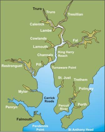

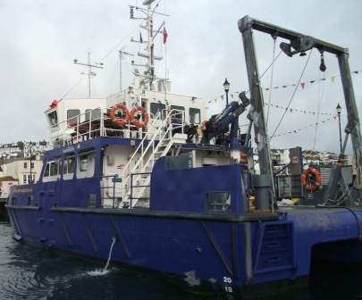
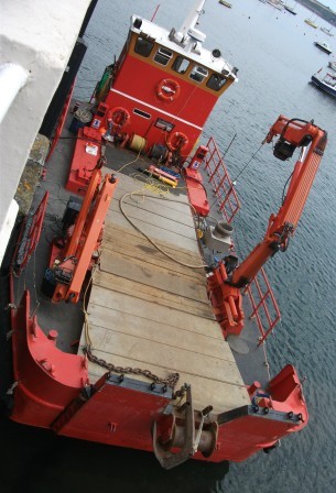
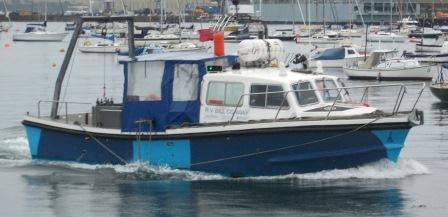

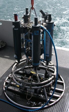
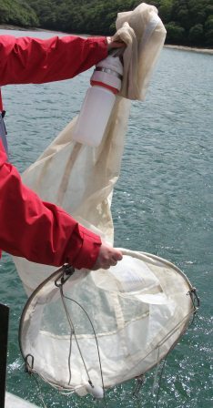
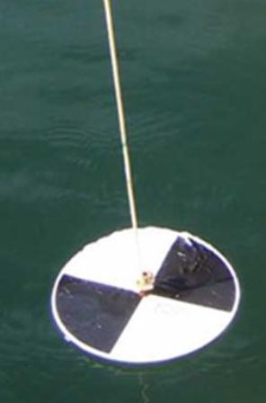
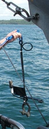
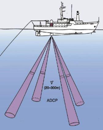
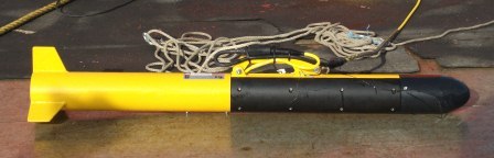
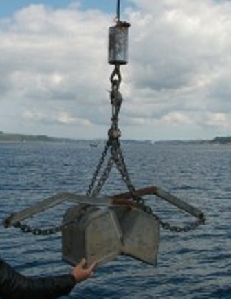
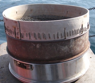
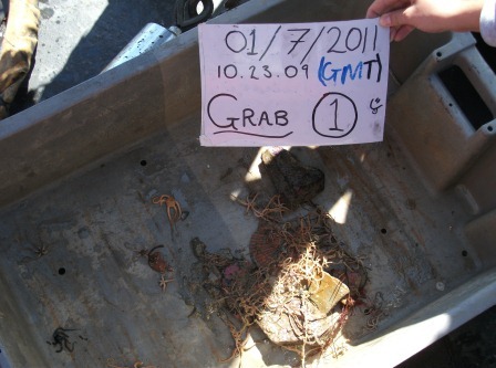
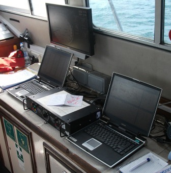
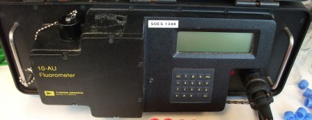
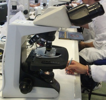
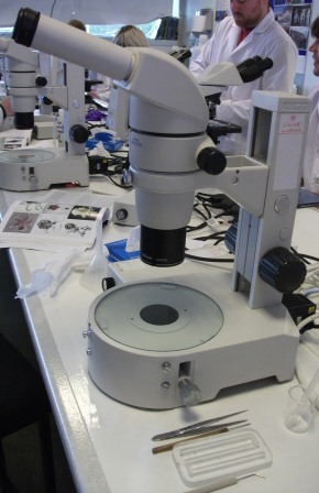
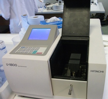
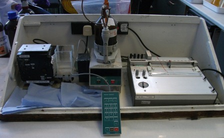
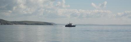


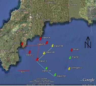


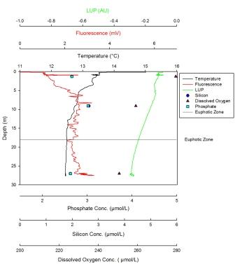
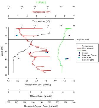
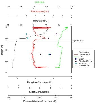
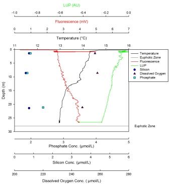
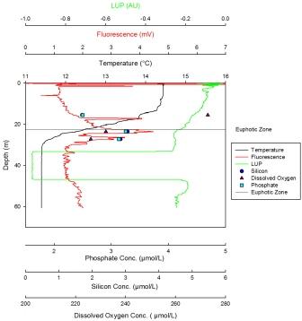
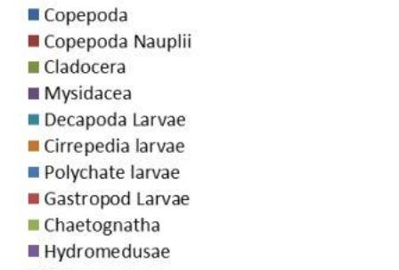
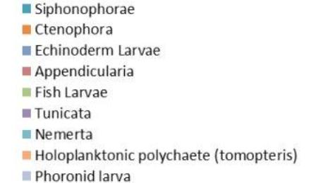
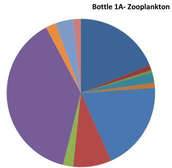
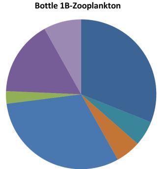
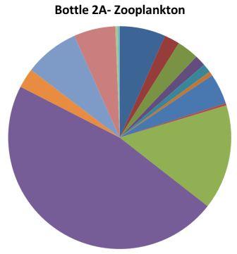
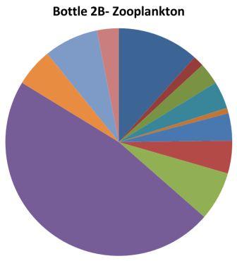
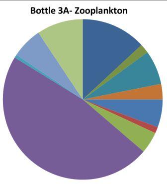

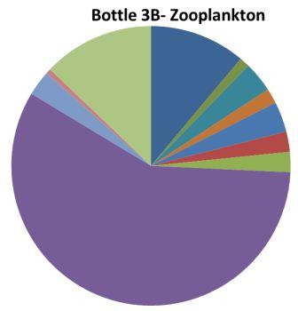
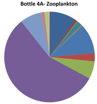
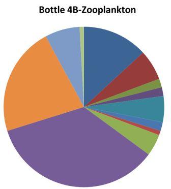
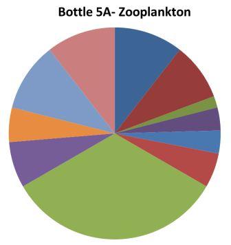

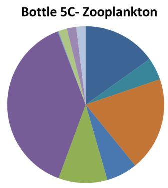
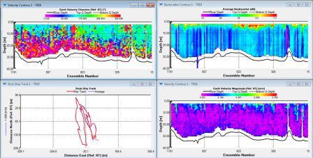
.jpg)
.jpg)
.jpg)
.jpg)
.jpg)
.jpg)
.jpg)
.jpg)
.jpg)

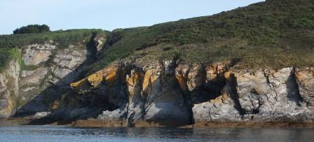


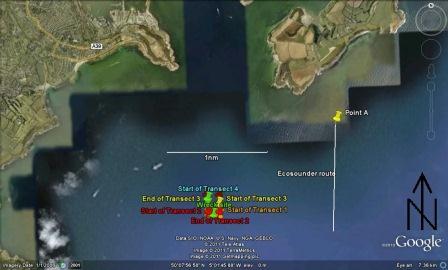
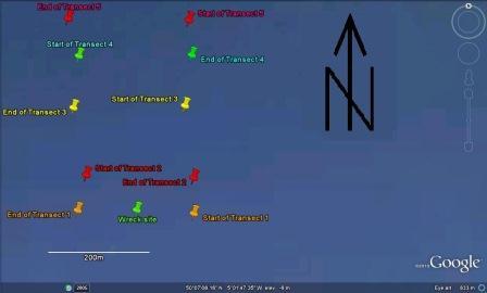
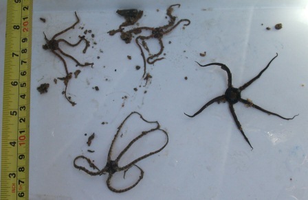
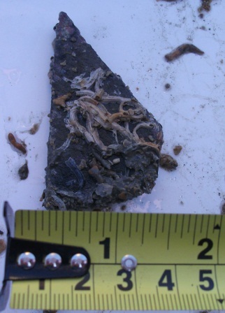

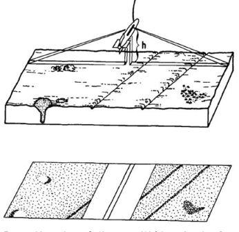 (Able
et al, 1987)
(Able
et al, 1987)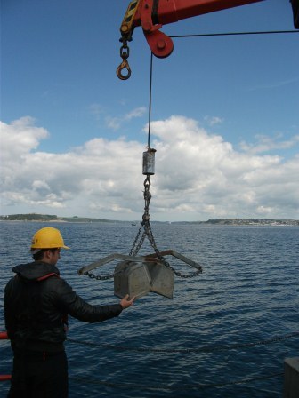
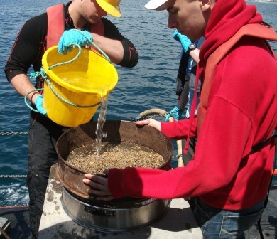
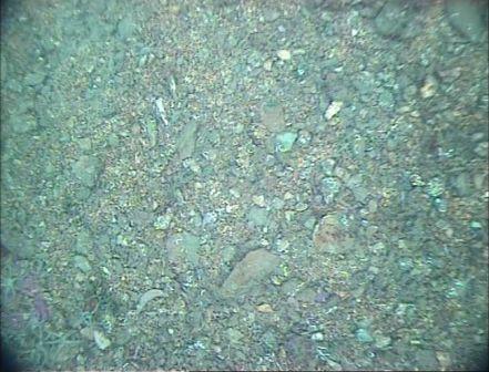

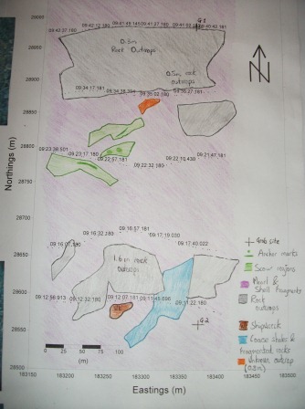
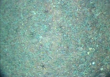
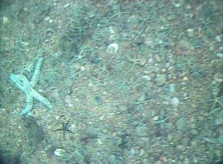
.jpg)