|
|
Group 9 |
 |
|
Samuel Buckley Simon Moore James Bell Katie Quaeck Daisy Chamberlain |
 |
Rebecca Hampshire Kathryn Weir Jake Baxter Ruth Throssell Nikoletta Sidiropoulou |
|
|
Group 9 |
|
|
Samuel Buckley Simon Moore James Bell Katie Quaeck Daisy Chamberlain |
|
Rebecca Hampshire Kathryn Weir Jake Baxter Ruth Throssell Nikoletta Sidiropoulou |
|
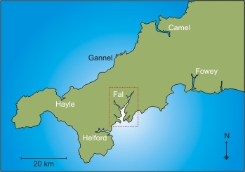
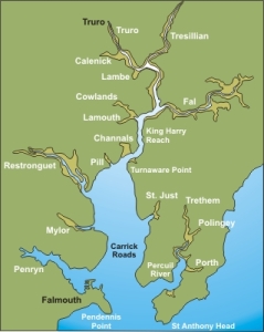
The Fal estuary is found on the southwest coast of Cornwall on the Roseland peninsular and is the UK’s largest estuary, with a macrotidal range of 5.3 metres. This region encompasses a wide range of habitats including sub-littoral mud and littoral rocky, sandy and muddy shores. The estuary is fed by a number of rivers, one the largest being the Truro river, and is also fed by several tidal creeks. The study conducted was implemented as a multi-parameter approach, being concerned with the physical, chemical and biological composition of the water as well as the benthic topography and dominant taxa associated with the estuary bed. The offshore and estuarine pelagic surveys documented the vertical profiles of physical features (i.e. temperature, light attenuation etc.) in situ, primarily via the use of a CTD profiler (or YSI multi-probe in unfavourable conditions) Water samples from predetermined depths were taken to measure the change in chemical components with depth (e.g. O2, N, Si & P). In addition to the depth profiles, a horizontal profile along the estuary was carried out to discern the mixing relationship of certain chemical parameters (Nitrite, Phosphate and Silicon) for subsequent lab analysis. The biological component of this survey concentrated on the relative abundance of zooplankton taxa . A geophysical survey was also carried out, which mapped the benthic habitat of Carrick Roads. A sidescan sonar was used along four transects in the area to visualise the seafloor, with video analysis and grab samples to investigate the benthic fauna present.
|
 |
 |
|
Figure 1.1: Map of Cornwall |
Figure 1.2: The Fal Estuary |
 |
 |
 |
|
Figure 2.1 |
Figure 2.2 |
Figure 2.3 |
|
R.V Callista is a twin hulled research vessel owned by the University of Southampton. It is 19.75 metres long, has a maximum breadth of 7.40 metres with a draught of 1.8 metres (fully loaded). She has a maximum speed of 15 knots, can carry a total of 30 people and has an SWL of 4 tonnes. |
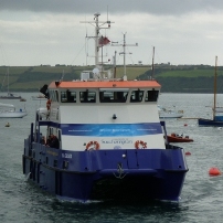
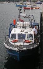
R.V Bill Conway is a small research vessel owned by the University of Southampton. At 11.74 metres long with a breadth of 3.96 metres, it draws 1.3 metres (fully loaded) and has a gross tonnage of 8.4 tonnes. R.V Bill Conway has a maximum speed of 10 knots and can carry a total of 12 scientists along with a skipper. |
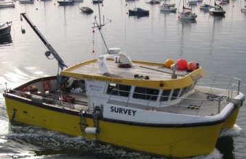
S.V Xplorer is a twin hulled diving support vessel owned by FD Marine Ltd. She is 12m long, 5.2m wide and has a draught of 1.2m. Xplorer is able to carry a load of 4 tonnes and is licensed to carry 12 passengers along with 2 crew members. She is powered by two 430hp engines allowing a top speed of 25 knots and a comfortable cruising speed of 18 knots. |
|
ADCP |
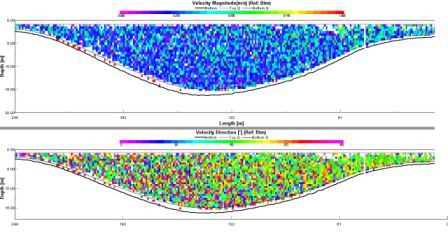 Figure 3.1 |
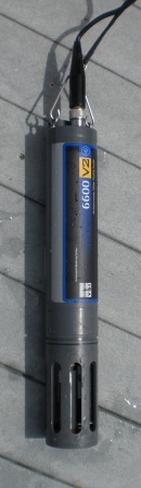
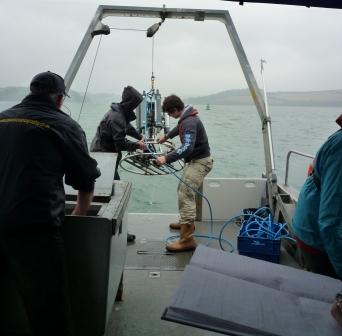
CTD |
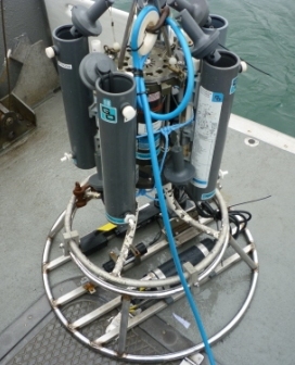 Figure 3.2 |
Plankton/Bongo Nets |
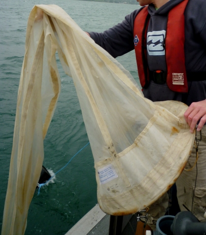 Figure 3.3 |
|
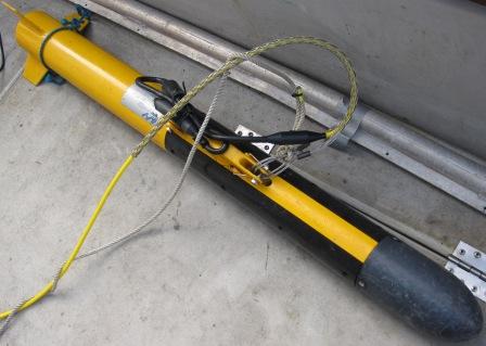
The ADCP uses Doppler shift to determine current velocity and direction of a flow within a water body. Particles, such as zooplankton and suspended particulate matter, can also be detected via backscatter. Particles moving away from the ADCP create a lower frequency, and those moving towards it will have a higher frequency. |
The CTD is an instrument which is lowered down through the water column. It measures conductivity (salinity), temperature, pressure, fluorescence and irradiance against depth. Data are continually recorded and automatically transferred to an onboard computer. The CTD is attached to a rosette which allows Niskin bottles to be closed at set depths. |
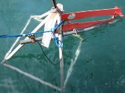
Plankton nets can be used to sample vertically within the water column, towed behind moving vessels or attached to static moorings (eulerian) to sample with the local flow/current. Nets vary in mesh size, and a 200µm was used for this study. The net is equipped with an impellor which has a 5 digit counter which allows calculation of the volume of water being filtered into a 500ml collecting bottle. |
|
Secchi Disk |
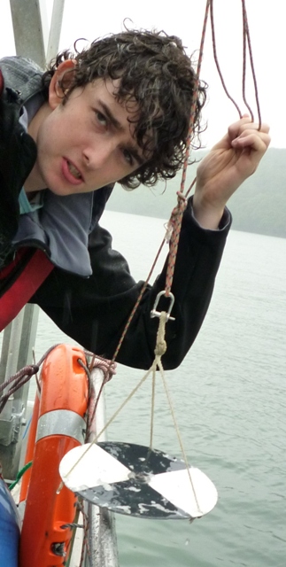 Figure 3.4 |
Sidescan Sonar |
Figure 3.5 |
T/S Probe |
Figure 3.6 |
|
A Secchi disk is a simple yet effective instrument used to estimate the depth of the euphotic zone. It consists of a circular piece of metal/wood with each quarter painted black or white alternately. An observer lowers the weighted disk, attached to a line, through the water column. The depth at which the secchi disk can no longer be seen is roughly 1/3 of the depth of the euphotic zone. |
The sidescan sonar was used onboard S.V Xplorer. It is GeoAcoustics Dual Frequency Sidescan Sonar which is towed along a predetermined track. An acoustic pulse is emitted by the instrument which reflects off the seabed and continuous data is recorded. More energy from the pulse is absorbed by mud and silt leading to a lower return signal, whereas coarse sediments have the opposite effect producing a higher return signal due to greater reflection. |
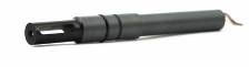
The temperature and salinity (T/S) probe is an instrument used for measuring temperature (thermister) and salinity (conductivity). It can be manually deployed from the side of a vessel and is often used when conditions are unfavourable for CTD deployment.
|
|
Van Veen Grab |
Figure 3.7 |
Video Camera |
Figure 3.8 |
YSI probe |
Figure 3.9 |
|
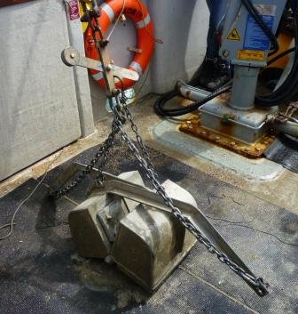
The Van Veen Grab is a claw mechanism which is lowered to the seabed closing upon contact with the sediment, obtaining a sample “grab”. Although small particles may be lost through the claw, the Van Veen Grab is a simple and reliable instrument, especially useful in soft sediment. It may also be used to examine benthic sea floor communities. |
A waterproof camera allows visual examination of the sea bed and is used alongside the Van Veen Grab. The camera can check for rare species and is therefore of qualitative value. Although the video cannot collect quantitative data, it allows verification of habitat type. |
The YSI probe is an electronic instrument which is used to measure salinity, via conductivity, and temperature using a thermistor. The probe also measures percentage oxygen saturation, turbidity and pH, with depth. A YSI probe is often used when unfavourable conditions prevent CTD deployment. |
![]()
![]()
![]()
![]()
![]()
![]()
![]()
![]()
![]()
|
The concentration of dissolved oxygen, nitrate, phosphate and silicon of each water sample was calculated in order to investigate the relationship between these chemical properties and chlorophyll at various positions and depths, ranging from shallow estuarine environments to deep offshore stations. The following techniques were used: |
|
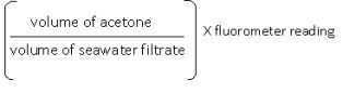
Chlorophyll: Once the sea water had been filtered, 6ml of 90% acetone was added and these were frozen over night rather than sonicated as this negated the use of a sonicator. The acetone and chlorophyll solution was pour into a cuvette and placed in the fluorometer in order to read off the chlorophyll value measured in µg/L. To calculate the chlorophyll content in seawater the following calculation was implemented:
|
|
Dissolved Oxygen: Water samples from thefour CTD stations along the estuary were collected in glass bottles, and treated with 1ml of both manganese chloride and alkaline iodide whilst on board the vessel. The samples were stored submerged in seawater to reduce contamination by atmospheric oxygen. Samples were later analysed in the laboratory using the Winkler technique (Grasshoff, K.,1999) using 0.22moles of sodium thiosulphate. |
|
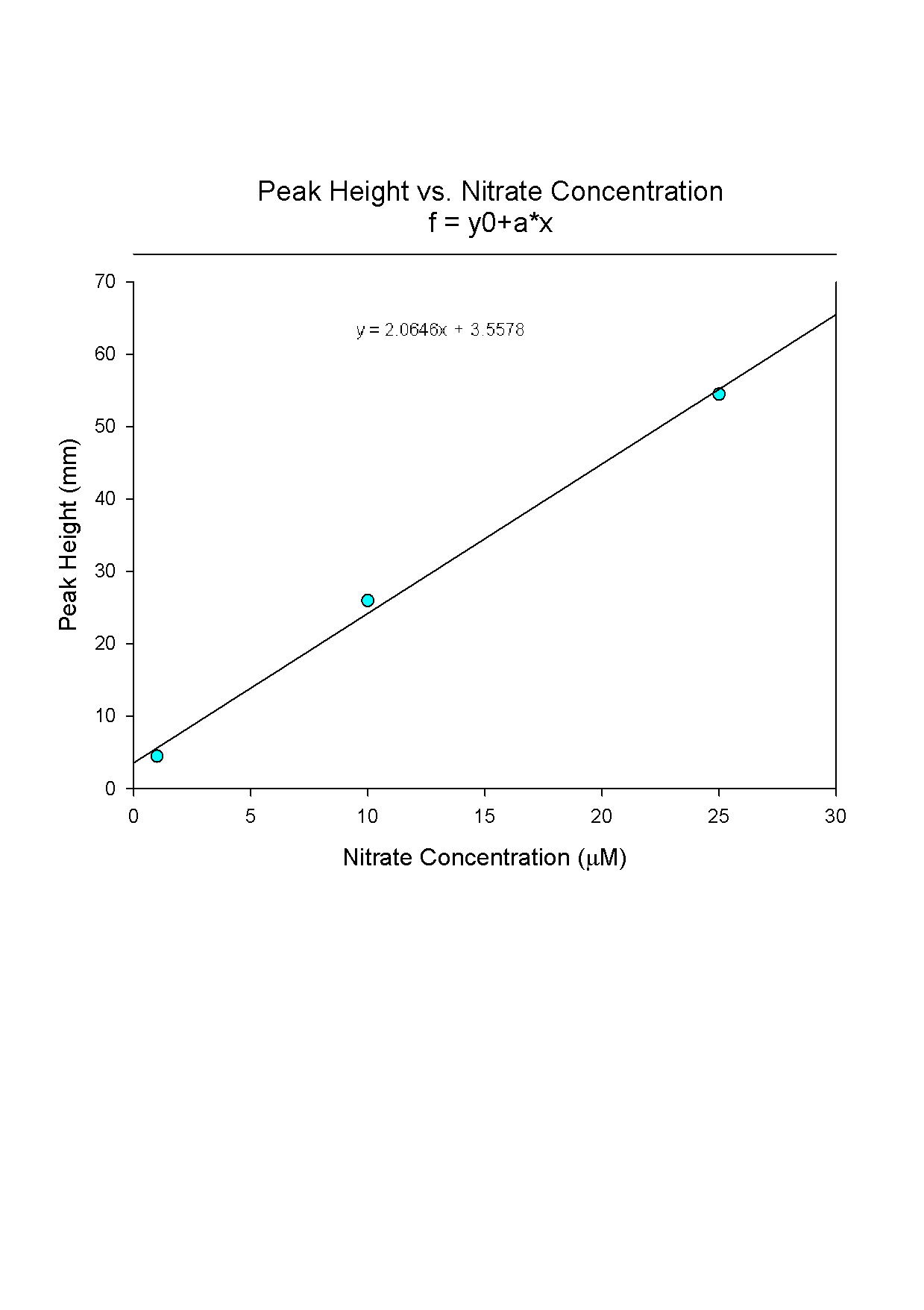
Nitrate: Nitrate concentrations of water samples were determined using flow analysis. The reagents used were sulphanilamide (1%) and NEDH (0.1%), which were independently injected using a peristaltic pump system, along with artificial seawater. The flow rates were controlled by the diameter of the tubing. The reagents were added at a rate of 0.76ml/min and the artificial seawater at 1.02ml/min. This method measures Nitrite, therefore the sample passed through a copperised cadmium column, known as a redactor. This converted nitrate to nitrite. As nitrite concentration is generally low in seawater (…..%), minimal error was introduced by the method. Approximately 150 µl of each sample (determined by the length of the tube) was mixed with the reagents and artificial seawater (used as a blank) prior to recording of transmission. The heights of the peaks on the read-out were proportional to the sample’s transmission. To determine concentration, the transmissions of standards with known nitrate concentrations were used to produce a calibration plot. This method is outlined in Johnson et al, 1983. |
|
Phosphate: From each collected sample, and the riverine and intermediate salinity samples provided in the laboratory, 10ml was removed and used as a working sample. Ammonium Molybdate, Sulphuric acid, Ascorbic acid and Potassium antimonly tartrate were mixed at a ratio of 2:5:2:1 and 1ml of this solution was added to each working sample. These were then left for approximately one hour to allow colour development. The absorbance of each working sample was then measured using a Hitachi U-1800 spectrophotometer at wavelength 882nm. The phosphate concentration of each sample was then calculated with the aid of a calibration plot, produced using the absorbance of standards of a known phosphate concentration. |
|
Silicon: Two sets of standards were required in order to calculate the silicon concentrations of water samples collected during the estuarine survey. Concentrated standards (set A) were required for the samples collected from the Truro River, as riverine silicon concentration is generally greater than estuarine and off-shore samples (set B standards). The lack of precipitation in the days leading up to the time of sampling lead to reduced riverine input, contributing to the low silicon concentration of samples collected from the estuary. Dilute standards were prepared from standard stock concentrations: 35.6 mmol/L was diluted 10 times to make up working standard A, and 25 times for working standard B. Working standard A was then used to make up five different silicon concentrations (7.1, 17.8, 35.6 53.4 and 71.1 µmol/L) and six different concentrations were prepared from working standard B (1.4, 2.8, 7.1, 14.2, 21.4, 28.5 µmol/L). Two replicates of each concentration standard were also measured. For analysis of the samples collected during the offshore survey, four standards of known silicon concentration were prepared. 5Ml of each sample/standard was mixed with 2ml of Ammonium Molybdate and left for 10 minutes. A mixed reducing agent was then added and left to stand of 2 hours. The mixed reducing reagent (MRR) comprised of; Metol Sulphite, Oxalic Acid, Sulphuric Acid (50% v/v) and MQ water, added in a ratio of 10:6:6:8. These reagents were mixed together and 3ml was added to each of the water samples, standards, and blanks. Following a 2 hour standing period, the absorbance of the standards and samples was measured using a U5625 spectrometer at a wavelength of 810nm, and recorded. The silicon concentration of each sample was then calculated using a calibration plot constructed from the absorbance values of the standards of known concentration. This method is outlined in Parsons et al, (1984). |
|
Introduction and Method: The estuarine field work was carried out on the 01/07/10 onboard RV Bill Conway. The aim was to investigate how the physics, chemistry and biology of the Fal estuary change within the transition zone between riverine and coastal waters. To achieve this, temperature, salinity, turbidity and chlorophyll data were collected using a CTD. The YSI probe was used when conditions were unfavourable for the deployment of the CTD and an ADCP system was used to collect data on flow direction and velocity as well as suspended particulate matter. Water samples from rosette mounted Niskin bottles, and a continuous pumped surface supply, were taken to determine concentrations of nitrate, phosphate, silicon and dissolved oxygen allowing investigation of the horizontal and vertical distribution of these chemical components. All samples were filtered to remove phytoplankton, and these filters used to calculate chlorophyll concentration. The depth of the euphotic zone was estimated using a Secchi disk and photometer. ADCP data were collected along six transects spanning the width of the estuary at different positions along its length. In the middle of each transect, either the CTD or the YSI probe was deployed. Water samples were taken from the pump system with every 0.25 change in surface salinity.
Weather Conditions and Tidal State:
Transect Locations and Times: Station Locations and Times:
|
|||||||||||||||||||||||||||||||||||||||||||||||||||||||||||||||||||||||||||||||||||||||||
|
Biological |
CLICK TO ENLARGE IMAGES |
||||||||||||||||||||||||||||||||||||||||||||||||||||||||||||||||||||||||||||||||||||||||
|
Phytoplankton: Water samples collected during the estuarine survey were mixed with Lugols solution, and stored in bottles onboard RV Bill Conway in order to preserve planktonic organisms. In the laboratory the samples were transferred to settling tubes and left overnight. The following day 90% of the solution was removed with a vacuum pump and u-bend tube. The remaining sample was agitated to suspend phytoplankton. A 21ml sub-samples from each station were prepared on a Sedgwick Rafter chamber and observed under x400 magnification. Phytoplankton were identified and counted systematically within the grid on the chamber. A replicate count was carried out for each sample.
Zooplankton:
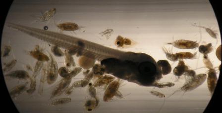
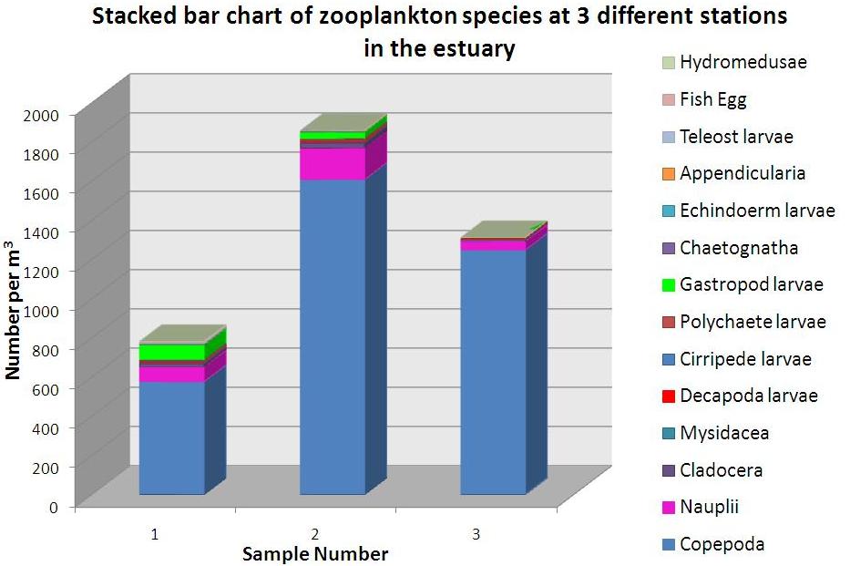
Three zooplankton net samples were taken from positions A, B and C in Fal estuary on 01/07/10. A 200µm mesh net with a 53cm diameter was towed for 5 minutes, at approximately 1m depth. Samples A and B were taken from the lower estuary and sample C was taken from the upper part of the estuary. Formalin was added to each sample in order to preserve its contents. Each litre sample was concentrated into 500ml bottle. Following homogenising by inversion, 5 ml of each sample was placed into a Borgorov chamber. Each zooplankton was identified and counted using a light microscope, and the procedure was repeated for each sample. The dominant taxa recorded include: copepods (and copepod nauplii), cladocerans and gastropod larvae, with calanoid copepods representing the vast majority of each sample - up to 20x more abundant than the next most common organism.
|
Figure 4.1: Fish Larvae and Copepods
Figure 4.2: Zooplankton Species in the Estuary |
||||||||||||||||||||||||||||||||||||||||||||||||||||||||||||||||||||||||||||||||||||||||
|
Chemical |
CLICK TO ENLARGE IMAGES |
||||||||||||||||||||||||||||||||||||||||||||||||||||||||||||||||||||||||||||||||||||||||
|
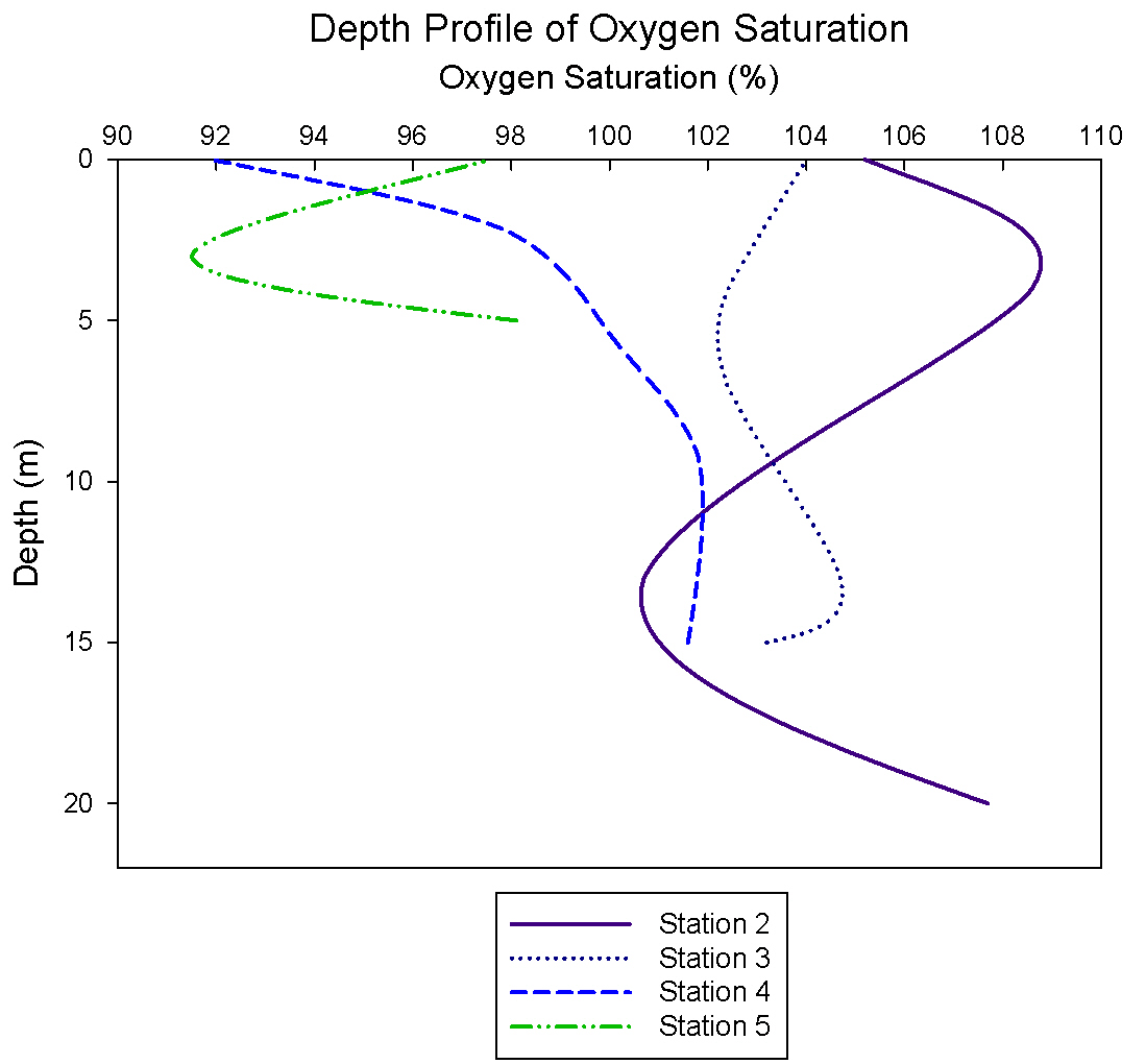
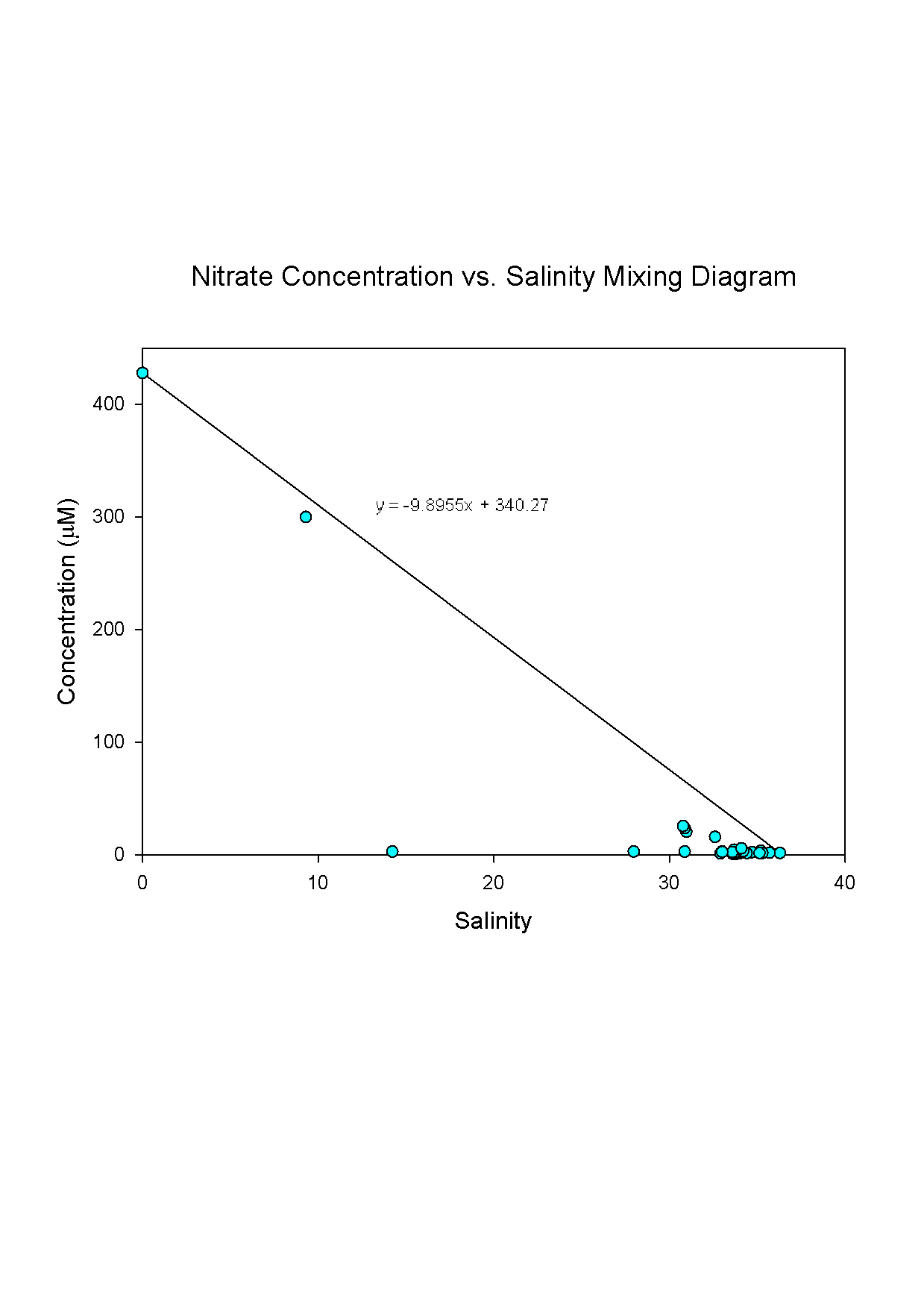
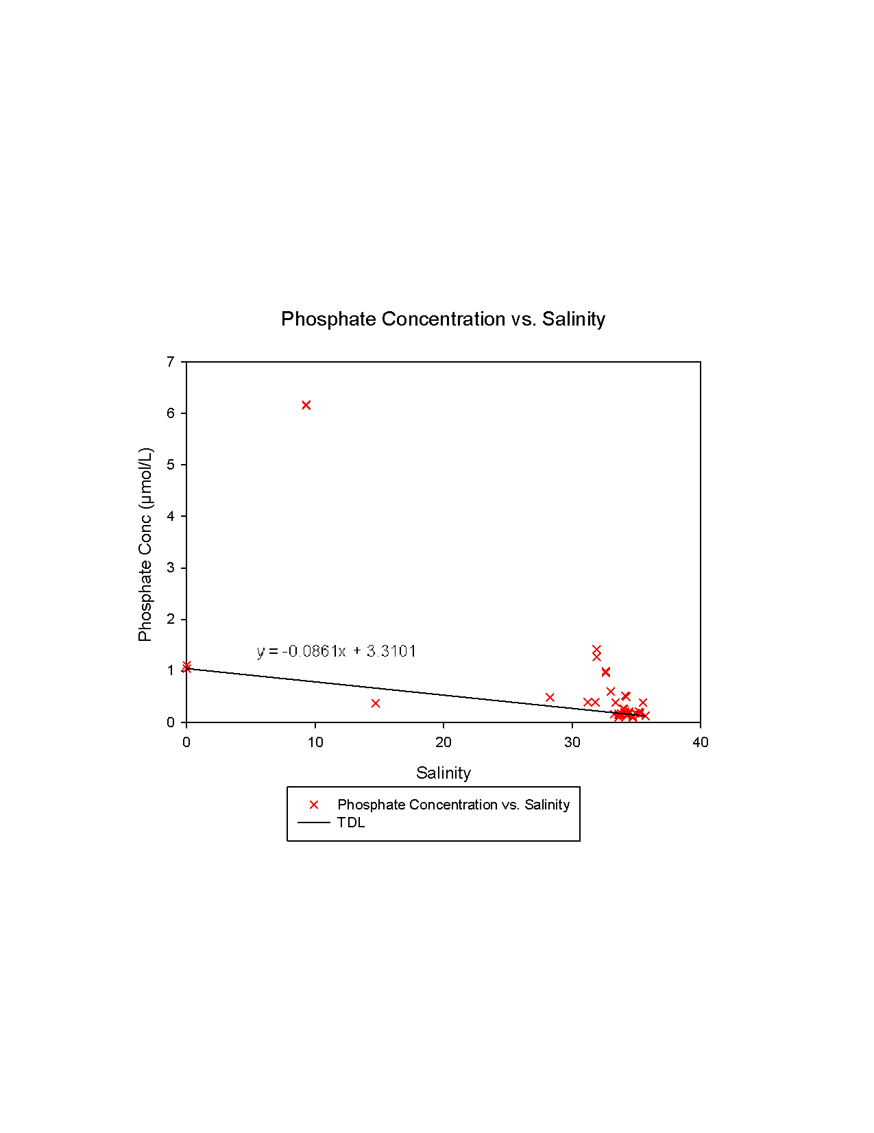
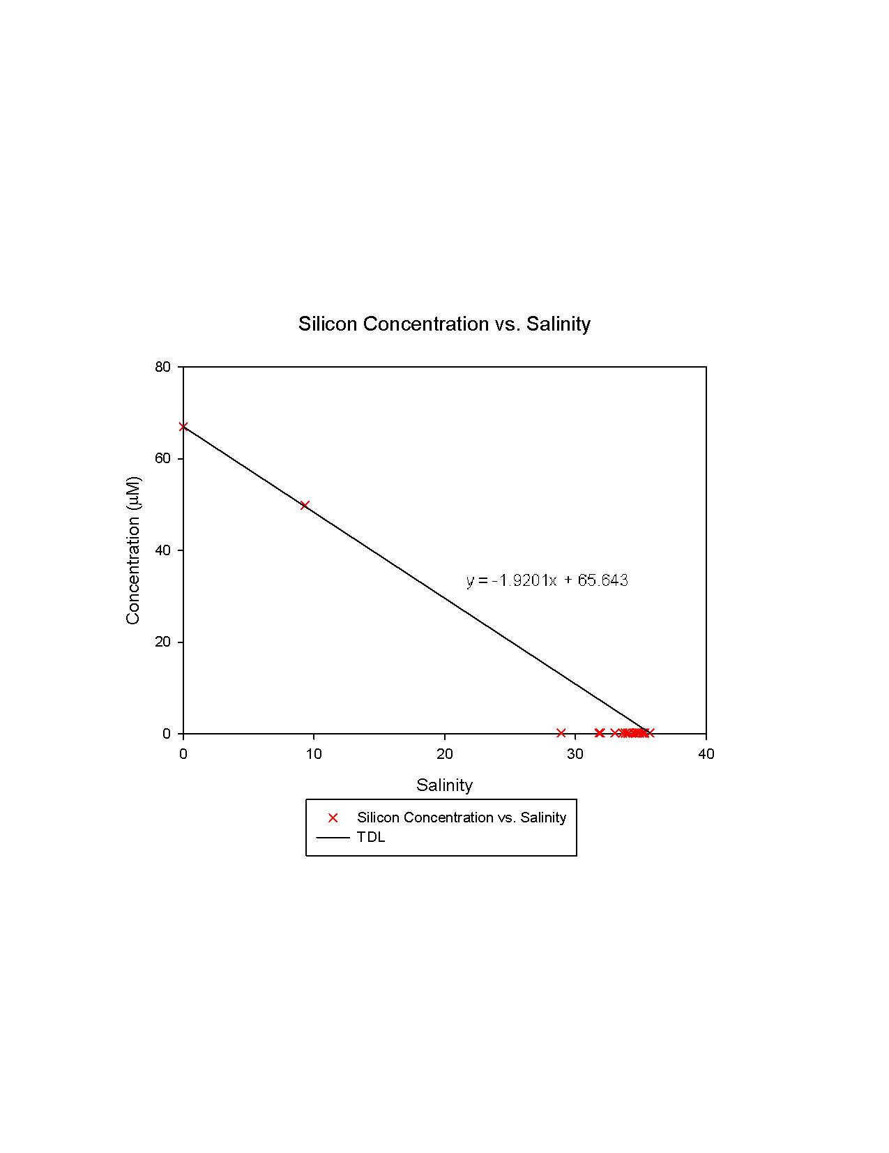
Dissolved Oxygen: As the survey advanced down the estuary, an overall increase in surface oxygen saturation, from 91.9% at station 4 to 105.2% at station 2, was observed. This may be attributed to an increase in the oxygen exchange rate with the atmosphere due to greater surface turbulence. At stations 3 and 5 oxygen levels decrease in the first few meters possibly as a consequence of zooplankton respiration, after which there is a gradual increase with depth. Station 4 has the lowest amount of surface oxygen suggesting a possible influx of deoxygenated water or sewage waste, with high biological oxygen demand (BOD). Station 2, located at the mouth of the estuary, shows the highest value of surface oxygen saturation. At 4.2m depth an oxygen saturation value of 108.5% was recorded, this value then decreases to 14m, which may be a result of zooplankton respiration and decomposition. There is little evidence that phytoplankton have an effect on the dissolved oxygen concentration, due to the lack of phytoplankton in the estuary. The depletion of phytoplankton is possibly due to heavy metal pollution within the estuary, as a result of the run off from the tin mines. The overall decrease in oxygen saturation from lower to upper estuary is likely to be due to the increase in nutrients associated with the pollution. Mixing Diagrams: Due to low rainfall, and consequently low riverine input to the estuary during the period leading up to sampling, a narrow range of salinities was observed. The majority of samples fell between salinities of 28.9 and 36.3. As a result of this, data points on the mixing diagrams are restricted to the higher salinity region, with few samples of low/intermediate salinities. This makes drawing conclusions regarding the behaviour of the chemical constituents within the estuary problematic. Sampling was also restricted to regions of the estuary easily navigable by RV Bill Conway. A theoretical dilution line (TDL) was plotted, linking the two data points with the highest and lowest salinities. When data points plot roughly along the TDL, conservative behaviour is observed and concentration varies linearly with salinity. However, non-conservative behaviour may be observed if addition or removal of the constituent occurs. Nitrate: Problems with the flow injection technique include those associated with the baseline from which the transmission peaks were measured. This occurred as background noise resulted in variation in the baseline’s position causing difficulty in peak height measurement. These deviations can be attributed to temperature fluctuations in the laboratory. Where nitrate concentration, and therefore peak height were low, it was difficult to distinguish between the “noise” and the true transmission peaks. Small differences in the transmission of the standards measured at the beginning and end of analysis were observed, possibly due to the reactor requiring recharging. In order to produce a mixing diagram, a riverine end-member was required. This sample was obtained from the Truro River (0 salinity). A sample of intermediate salinity was also obtained. The nitrate mixing diagram shows that the majority of samples had very low concentrations of nitrate, plotting below the TDL. Although nitrate appears to behave non-conservatively, the lack of low and intermediate salinity samples makes it difficult to determine whether removal of nitrate from the system was occurring. One intermediate salinity sample was obtained (14.7) from the surface during a CTD profile, however this appears to be an anomalous result as it does not relate to the other surface readings collected in the area. Phosphate: The phosphate estuarine mixing diagram shows a relatively high range of phosphate concentrations for a given salinity, with apparent non-conservative behaviour. There is an outlier at salinity 9.3, and this sample has an unusually high phosphate concentration of 6.16µmol/L. This sample was provided in the lab, representing an intermediate salinity data point. There is an apparent input of phosphate to the estuary here, possibly of anthropogenic origin from a source such as the sewerage works. Silicon: Figure 5.5 demonstrates that silicon concentration decreases with increasing salinity. The riverine end member, salinity 0, has a silicon concentration of 67.02µmol/L whereas the seawater end member, salinity 35.7, has a concentration of 0.20µmol/L. Silicon appears to act conservatively between salinities of 0 and 9.3 but as silicon concentrations at higher salinities fall below the Theoretical Dilution Line some silicon removal appears to occur. However, it was not possible to sample between salinities of 9.3 and 0 due to vessel restrictions, it is therefore difficult to determine whether removal is actually taking place. One problem arose from the technique used to determine silicon concentration of the water samples collected. The equation for the calibration curves obtained from the absorption of standards had intercepts of 0.2262 for the concentrated standards and -1.7116 for the diluted standards, rather than 0. This may have lead to inaccuracies in the silicon concentrations recorded for the collected samples, as an intercept of 0 is required to accurately calculate silicon concentrations. Nutrient Discussion: Upon analysis of the chemical data and their subsequent incorporation into depth profiles, several trends emerged between the estuary head and mouth. In concordance with the seasonality of phytoplankton abundance (Miller 2004), the investigation found low chlorophyll concentrations, particularly towards the seaward end and an average phytoplankton cell count of 0.33 cells ml-1. Interestingly, despite the chlorophyll concentration being an order of magnitude higher in the upper estuary compared to the lower end, the percentage saturation of oxygen shows a continual increase towards the seaward end, up to 108.5%. A possible explanation for this is the increase in turbulent surface mixing and bubble entrainment as exposure to wind stress increases. On the day of this investigation, sampling of most of the seaward area of the estuary had to be abandoned as the conditions exceeded the safe working limits (< Gale Force 6) of R.V Bill Conway. Samples were therefore only attainable within the shelter of the Fal estuary. Another potential reason for the discrepancy in oxygen saturation is high BOD (biological oxygen demand) in the upper estuary, as a consequence of nitrate and phosphate input from a sewage outflow in the Truro River. (Nitrate directive*) The decrease in chlorophyll concentration with distance downriver can be explained by a combination of two factors; an increase in zooplankton towards the seaward end, which increases the grazing pressure upon the phytoplankton and microbial component of the estuary, as well as the dilution, via mixing, and uptake of nutrients in the upper estuary by primary producers. Despite the lack of evidence for silica-secreting organisms, there is an apparent relationship between silicon concentration and salinity which cannot be accounted for solely by mixing. This suggests some component of biological uptake of silica, either by pelagic phytoplankton or sessile fauna such as poriferans. The increase in euphotic zone depth is also a measure of the decrease in phytoplankton abundance and over the course of the estuary increases its depth by a factor of 3, as a result of the decreasing influence of SPM (suspended particulate matter) In general it can be suggested that nitrate is the bio-limiting factor in surface waters toward the seaward end. In the upper estuary, the sewage outflow remains in sufficient concentrate to be non-limiting. It is therefore likely that light is the limiting factor. The estuary experiences a reduction in light attenuation (and increase in transmittance) toward the seaward end. With regard to trends in stratification, calculations of the Richardson number found that the upper part of the estuary was a well mixed system as a result of the low riverine freshwater input coupled with the strong wind stress on the day of the investigation.
|
Figure 5.1: Depth Profile of Oxygen Saturation
Figure 5.2: Nitrate Concentration vs. Salinity
Figure 5.3: Nitrate Concentration Peak Heights
Figure 5.4: Phosphate Concentration vs. Salinity
Figure 5.5: Silicon Concentration vs. Salinity
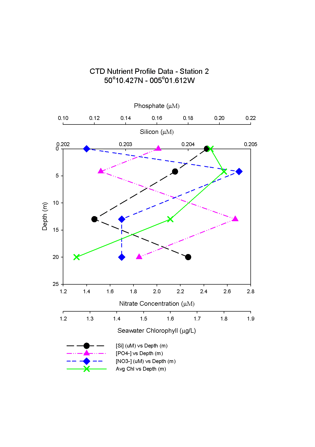
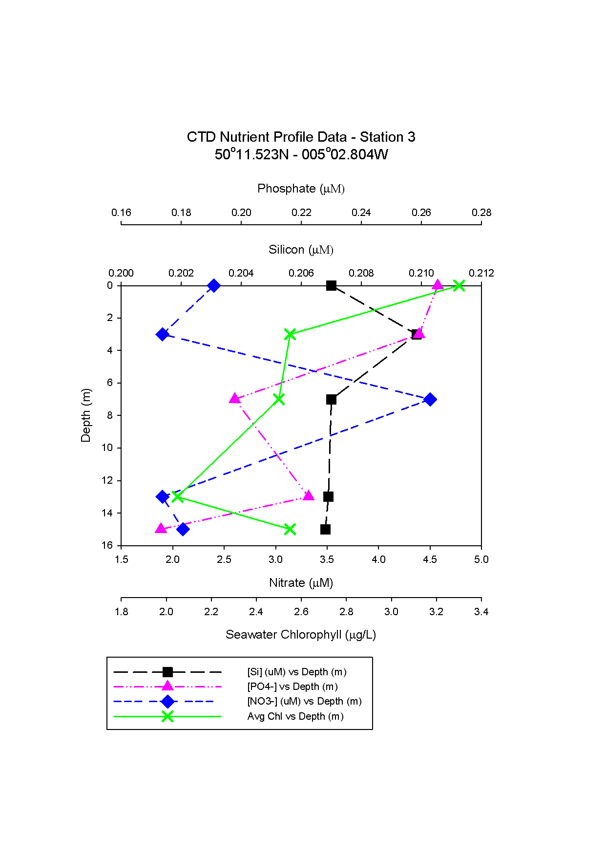
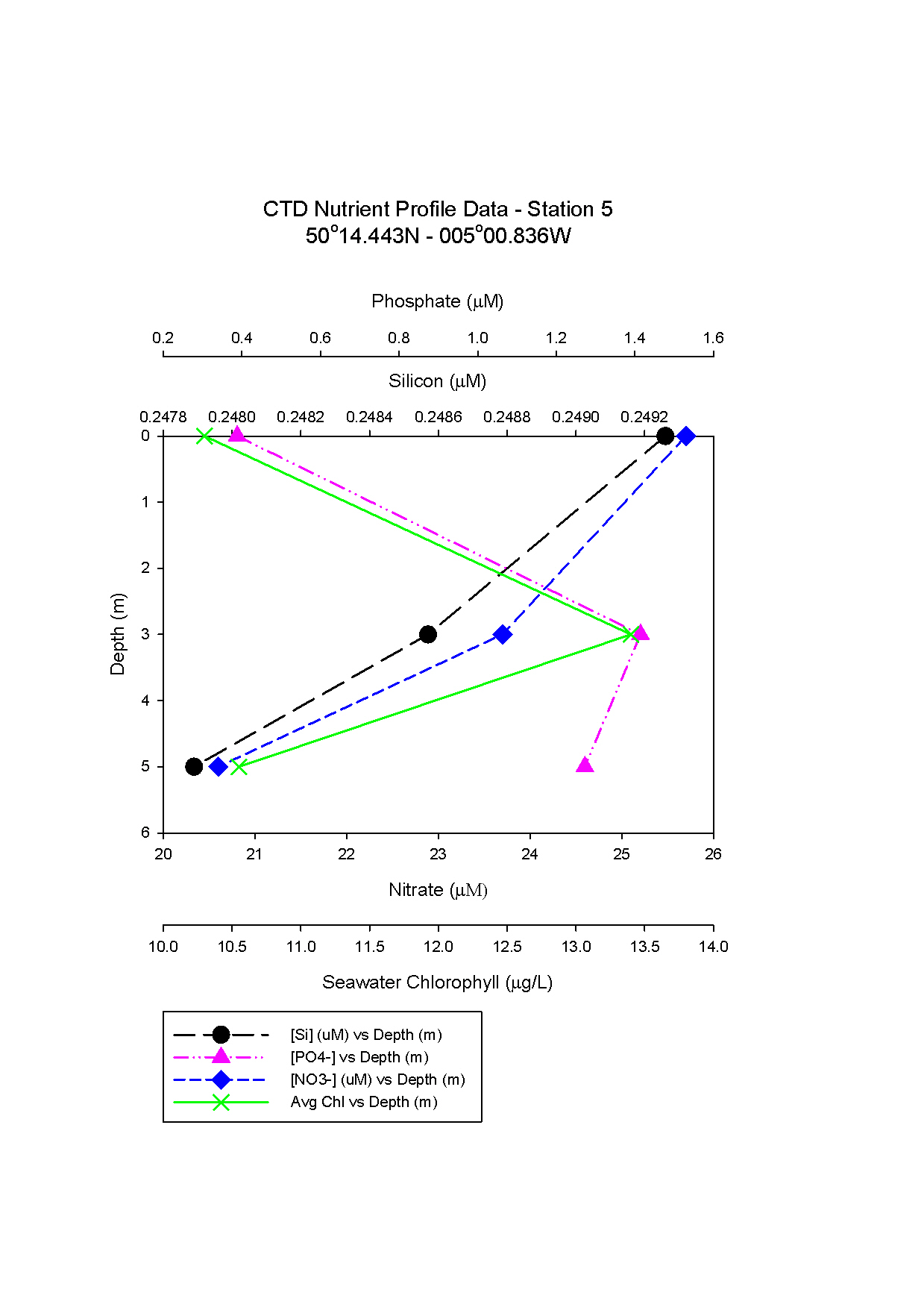
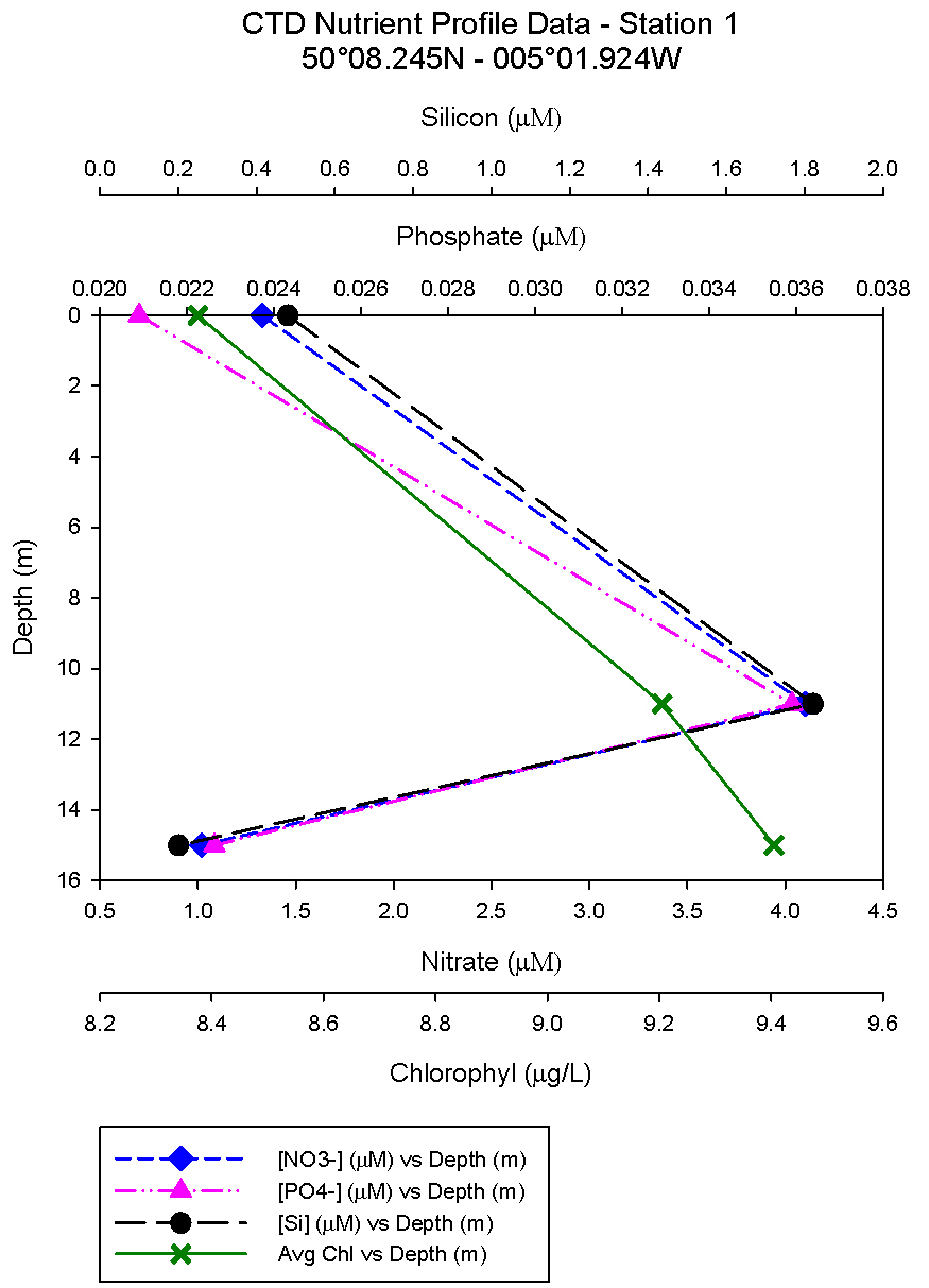
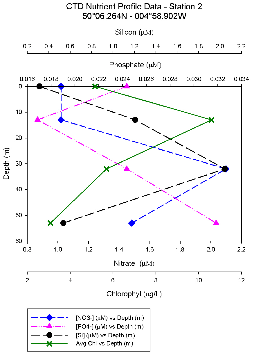
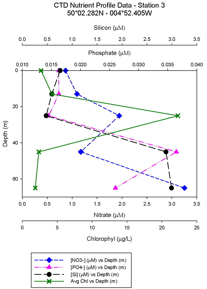
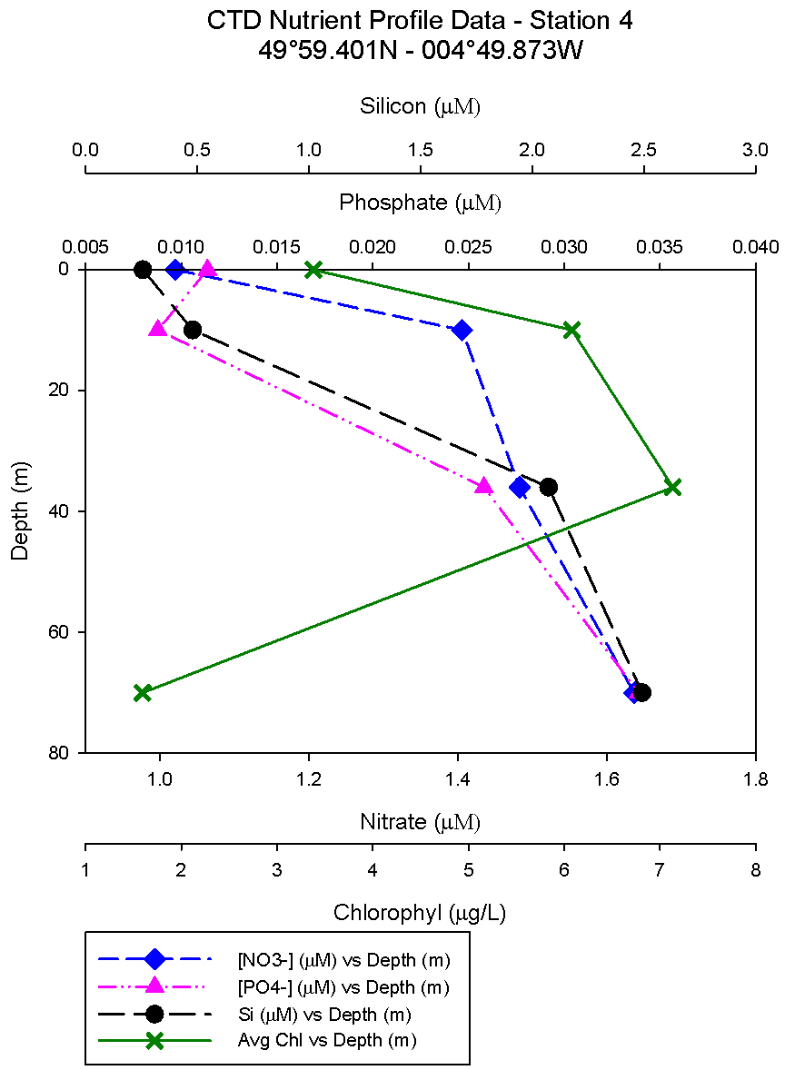
Figure 5.6: Station 2 Figure 5.7: Station 3 Nutrient Profile Nutrient Profile
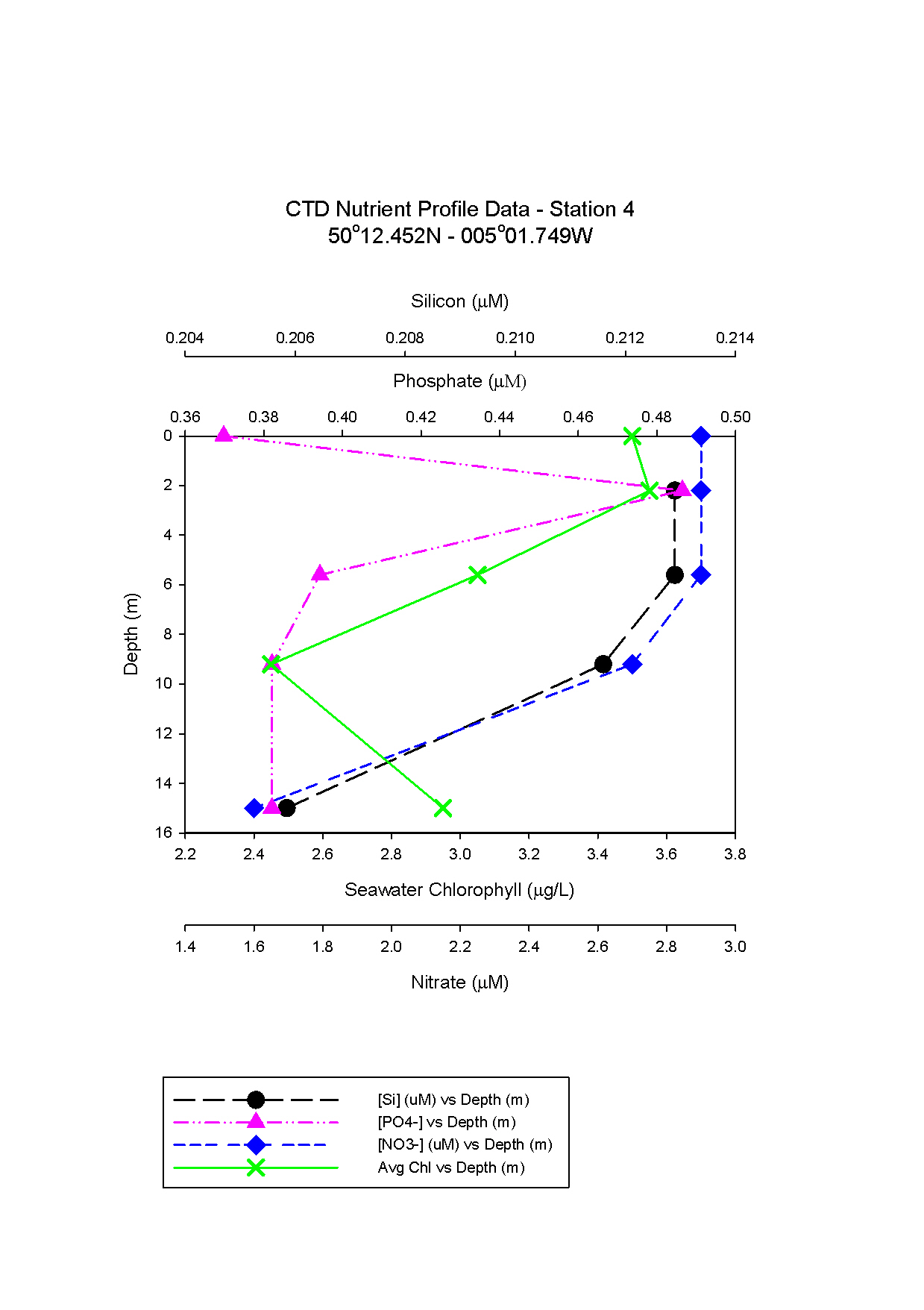
Figure 5.8: Station 4 Figure 5.9: Station 5 Nutrient Profile Nutrient Profile
|
||||||||||||||||||||||||||||||||||||||||||||||||||||||||||||||||||||||||||||||||||||||||
|
Physical |
CLICK TO ENLARGE IMAGES |
||||||||||||||||||||||||||||||||||||||||||||||||||||||||||||||||||||||||||||||||||||||||
|
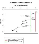
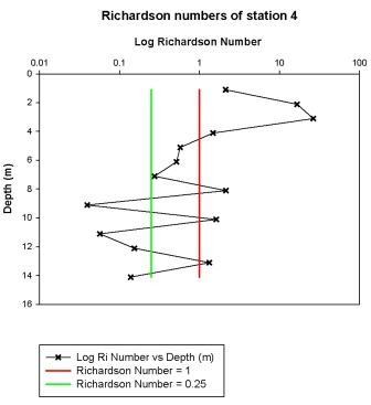
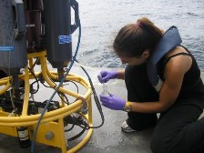
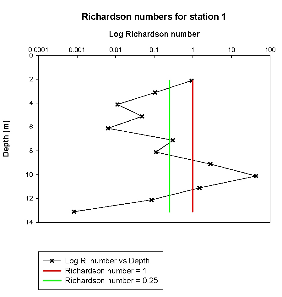
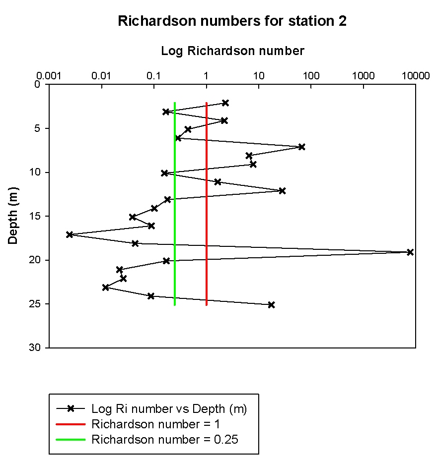
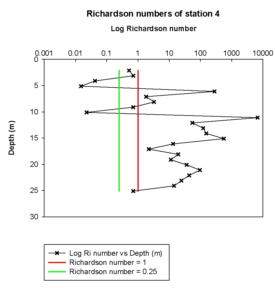
Light Attenuation Light penetration through the water column (photons/µmol/m²/s) is measured by a photometer . 6 stations were sampled along the length of the Fal estuary and light attenuation increased toward the mouth. Chlorophyll concentrations were greater toward the riverine end, with attenuation decreasing through the water column. Station 2 showed rapid attenuation of light, which may be due to wind stress resulting in mixing, thereby increasing turbidity of the surface layer. A problem that was encountered was that in some cases euphotic zone depth (1% light level) exceeded the depth of the deepest measurement. The slope of the log linear regression line equalled the light attenuation coefficient (k), which decreases up landward of station 2 as far as station 4. Higher k values were recorded at stations 5 & 6, indicative of the increase in phytoplankton biomass in the more nutrient rich upper estuary. Station 2 appears to have an anomalous high k value, possibly due to the increase in turbidity as a consequence of higher wind stress. Velocity Direction and Backscatter Transect 1 Transect one was carried out 25 minutes after high water (HW). At this time the channel is dominated by the ebb tide however the water over the shelf is not flowing in the same direction but instead the remainder of the flood tide is flowing in. The different flow over the shelf is due to the estuarine hydrograph as the water here is subject to more friction and therefore takes longer to change direction when the tides turn. Turbulent flow is observed in the surface waters of the channel, with mixing occurring between the ebb and flood tide. When this transect was surveyed, water flowed out through the narrowing mouth leading to increased friction and eddying compared to transect 2, located further up the estuary. The backscatter profile shows high values of approximately 80dB in the surface waters above the channel, indicating the presence of zooplankton. Below 15 meters, backscatter values fall 65dB, this can be related to the absence of zooplankton here. Transect 2 Transect 2 is located upstream of transect 1, in a wider section of the estuary 0.75 hours after HW. The ebb flow dominates the channel and surrounding shelves at this stage of the tidal cycle. The station 2 backscatter profile displays high values at the surface waters and low values below 10meters within the main channel, similar to station 1. Transect 3 Transect three is taken at the upper reaches of the Carrick Roads 2 hours after HW. The average flow direction reflects the ebb tide, with some turbulent flow over the shelves. High backscatter values, ranging from 70 to 80 dB, was recorded in the top 2meters of the water column and can be related to surface wave action. On the west side of the channel, backscatter values of 75 - 80 dB were recorded throughout the water column. This, combined with high turbulence values seen in at this position, is indicative of the re-suspension of sediments thus increasing the backscatter. Transect 4 Transect 4 was carried out in the River Fal, landward of Carrick Roads 3 hours after HW. Over this transect the ebb tide dominated the flow however some eddying was observed at the water-bed interface due to friction. The backscatter values for transect 4 remain at a constant low level, throughout the water column. However, there is an area of high backscatter, with values of approximately 80 dB, on the west side of the channel in the bottom waters. This can be attributed to turbulence resulting in sediment resuspension. Transect 6 Transect 6 was taken in the same location as transect 3 but only over the channel section due to the shelves on either side being too shallow. The data was collected 5 hours after high water and this is reflected in the average flow which is in the direction of the ebb tide. On average the backscatter over the transect is uniform with some regions of higher backscatter at the surface likely due to wave action. The Richardson Number (Ri) is a dimensionless ratio between the change in density gradient and velocity shear with depth and can be calculated using the following equation (Knauss, 1997):
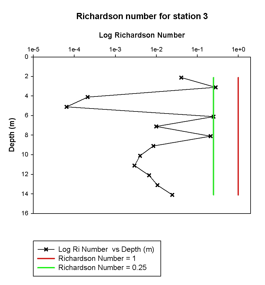
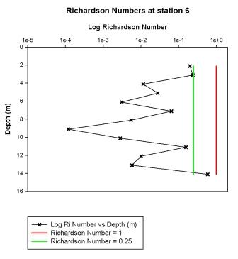
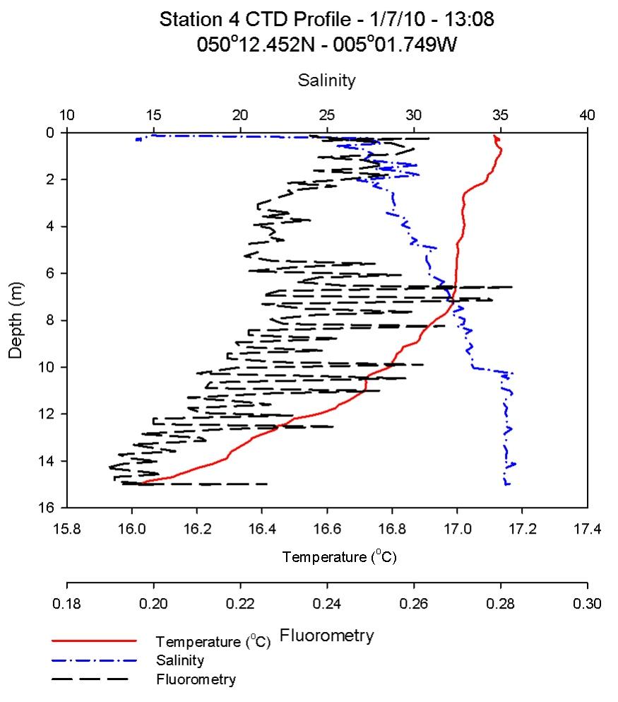
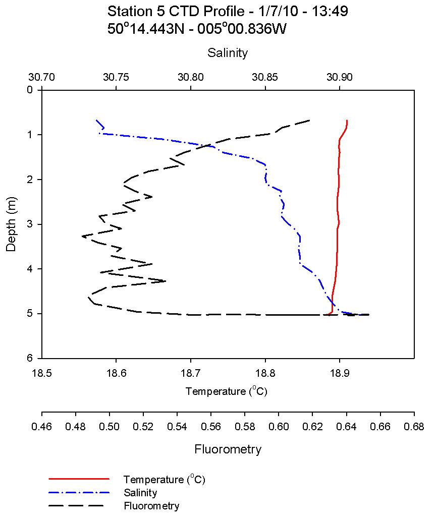
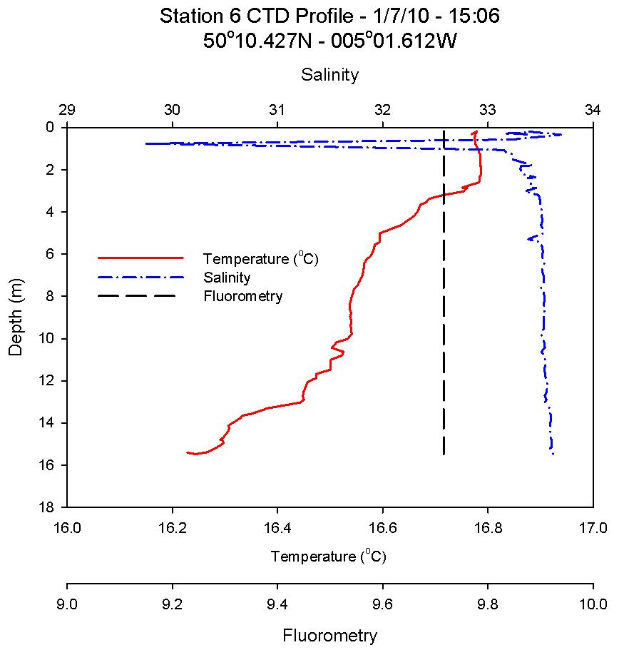
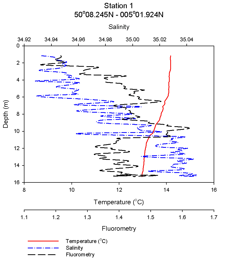
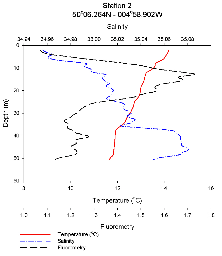
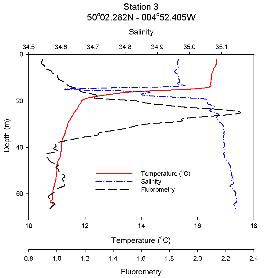
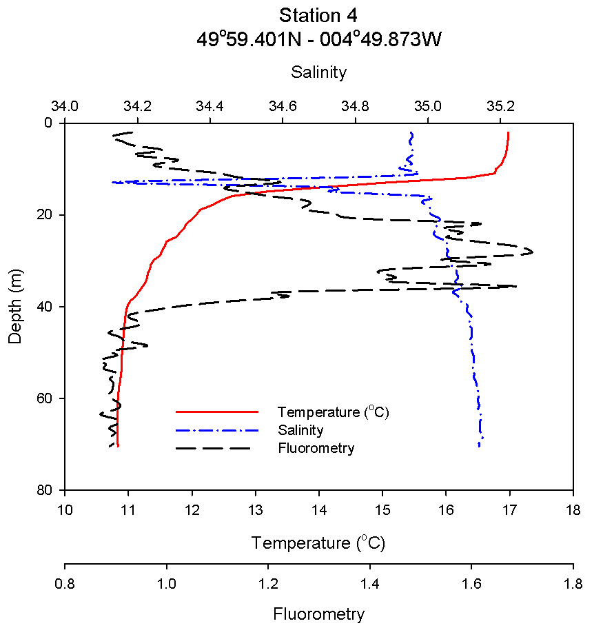
Where g is gravity, ρ is density, dρ is the change in density, and du is change in velocity. The water column was divided into 1m layers in order to calculate the change in density and velocity. Values recorded between 0 and 0.25 indicate gravitationally unstable water where mixing occurs; shear flow instability develops with values between 0.25 and 1; and values above 1 indicate that the flow is stable. The ‘du’ values were calculated using the VM and velocity direction from the ADCP data. Where the VM had approximately the same direction the values between the 1m layers were subtracted from each other. When the flow between layers varied in direction the VMs were added together as variation in direction of flow leads to the generation of shear. For the estuary the CTD raw data did not include water density therefore a formula from an UNESCO technical paper written by Fofonoff and Millard (1983) was used to calculate density using the depth, temperature, and salinity. Station 5 was a stationary station taken in a shallow location therefore due to a small data set the RI has not been calculated. The YSI Probe was used to collected data down to 9m at station 1 due to safety reasons producing a small dataset, therefore Ri values have not been calculated as they would be representative of the water column. Richardson Number at stations along the estuary For station 2 CTD values where collected down to an approximate depth of 20m. Values indicating stability were found between 1-3m; a value indicating shear flow instability was found between 3-5m and 6-9m; and the rest of the water column had values below 0.25 suggesting well mixed layers. For station 3 CTD values were collected down to an approximate depth of 15m. No values indicating stability were found. Between 2-3m there was a value indicating shear flow instability and the rest of the water column was well mixed. For station 4 CTD values were collected down to an approximate depth of 15m. Values indicating stability were found between 1-5m, 9-10m, and 12-13m; values indicating shear flow instability were found between 4-7m; and the remainder of the Ri values suggest well mixed conditions between the other layers. For station 6 CTD values were collected down to an approximate depth of 14m. One value found at 13-14m indicated shear flow instability. The remainder of the Ri values were below 0.25 indicating a well mixed water column. In conclusion, station 3 and station 6 were taken in the upper region of the Carrick Roads and exhibited well mixed conditions. Station 2 taken in the mid section of the Carrick Roads and contained some stability in the upper layers however these higher RI numbers were due to the difference in VM rather than density. Station 4 located in the upper estuary exhibited the greatest stability as expected due to the greater variation in salinity with depth. Water Column Structure As the survey advanced up the estuary, an increase in temperature was observed; from 15.26⁰C at station 1 (seaward end) increasing to 18.91⁰C at the riverine end. A general increase in salinity was observed toward the mouth of the estuary, as seawater inundation increases and the effect of freshwater input is reduced. The estuary appeared to be well mixed throughout, with little of the haline stratification one would expect to observe in an estuarine system. This can be attributed to the relatively low rainfall in the period prior to surveying. Physical profiles showed a maximum temperature and salinity difference, between surface and seabed, of 1.1⁰C and 0.5, with the exception of station 4. Here a large decrease in salinity of 7.9 between 0.2m and 15m was observed, which is likely to be an anomalous result attributed to instrument error. Fluorometry measurements show relatively constant chlorophyll concentrations at stations 3 and 4, with readings of approximately 0.25µg/L at the surface, falling to 0.20µ at 16m. Chlorophyll concentration appears to increase between stations 4 and 5, with 0.62µg/L at the surface falling to 0.5µg/L at 5m. N.B. Fluorometry readings obtained at station 2 and 6 show constant readings of 9.72µg/L throughout the water column. Once again, this measurement is unlikely to be an accurate reflection of chlorophyll concentration and is possibly due to instrument error.
|
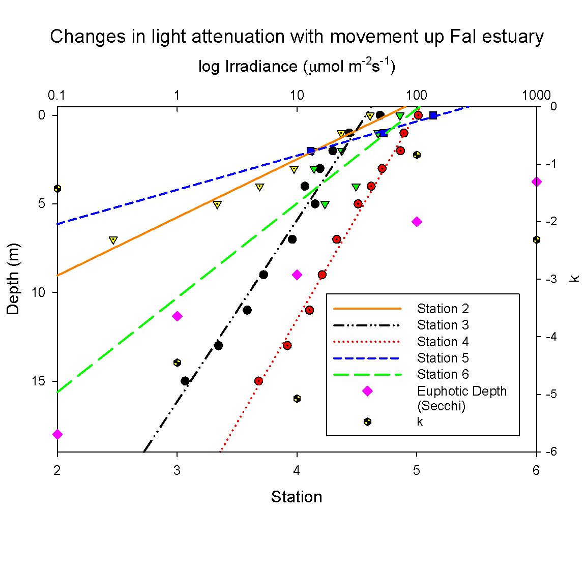 Figure 6.1: Light Attenuation in the Fal Estuary
Figure 6.2: Velocity Figure 6.3: Velocity Direction at Transect 1 Direction at Transect2
Figure 6.4: Velocity Figure 6.5: Velocity Direction at Transect 3 Direction at Transect4
Figure 6.6: Velocity Direction at Transect 6
Figure 6.7: Ri Number Figure 6.8: Ri Number Station 2 Station 3
Figure 6.9: Ri Number Figure 6.10: Ri Number Station 4 Station 6
Figure 6.11: Station 1 Figure 6.12: Station 2 YSI Profile CTD Profile
Figure 6.13: Station 3 Figure 6.14: Station 4 CTD Profile CTD Profile
Figure 6.15: Station 5 Figure 6.16: Station 6 CTD Profile CTD Profile
|
||||||||||||||||||||||||||||||||||||||||||||||||||||||||||||||||||||||||||||||||||||||||
|
Introduction and Method Conditions in the Western English Channel during the summer months are such that the waters become thermally stratified. The extent of this stratification is determined by water depth (h) and tidal strength (u). These parameters can provide an indication of the level of stratification, estimated using the following equation: h/u³ (Pingree & Griffiths, 1978). Further inshore, the thermocline is forced upwards by the shoaling bathymetry, leaving coastal waters well mixed. With development of a thermocline, associated with an increase in ambient air temperatures and a decrease in wind mixing, algal growth results in nutrient depletion in the upper waters. Nutrients may not be replenished by the deep waters due to development of the thermocline, and the extent of interaction between the two layers is dependent on the strength of this stratification. The aim of the offshore investigation was to establish the relationship between stratification and distance from shore. Water samples were collected onboard R.V. Callista, allowing calculation of dissolved oxygen, nutrient and chlorophyll concentration and plankton abundance. Data relating to temperature, salinity, depth, velocity and light attenuation were also collected using a CTD and ADCP. Four stations increasing in distance offshore, from Black Rock cardinal marker to a approximately 12nm offshore, were sampled. At each station the CTD was deployed and samples were taken from discrete depths. Bongo nets were deployed to vertically sample zooplankton through the water column. Additionally, a Secchi disk allowed estimation of the euphotic zone depth at each station. Between each station, an ADCP survey was carried out.
Weather Conditions and Tidal State:
|
||||||||||||||||||||||||||||||||||||||||||||||||||||||||||||||
|
Biological |
CLICK TO ENLARGE IMAGES |
|||||||||||||||||||||||||||||||||||||||||||||||||||||||||||||
|
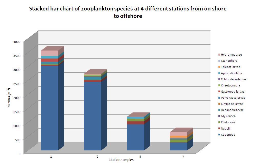
Phytoplankton Water samples were treated and stored using the same protocol implemented during the estuarine survey. A 10ml sample was then siphoned and 2ml was analysed on a Sedgwick Rafter slide. Figure 7.1 shows a table which details the phytoplankton types and the populations found in each station sample. The results show a decrease in phytoplankton abundance and diversity between stations 1 to 4. At station 1, five groups of phytoplankton were identified and replicate counts provided an average abundance of 12.5 cells/ml. Station 2 had the highest abundance (21.5 cells/ml) and diversity. Station 3 had low abundance and diversity, with a total of two phytoplankton cells counted. Finally, at station 4, a single phytoplankton cell was counted. The decrease in the abundance of phytoplankton with distance from the shore may be attributed to nutrient availability. The depth of coastal water decreases with proximity to the shoreline and the tidal currents force water shoreward. As bathymetry shallows, the thermocline is forced vertically upwards to the surface, thus nutrients are evenly distributed throughout the water column, and may be utilized by phytoplankton. With distance offshore mixing decreases, meaning fewer nutrients are mixed into the surface waters, therefore fewer phytoplankton can be supported within the system. This explains why low phytoplankton abundance and diversity was observed at station 4. Zooplankton Zooplankton samples were stored, preserved and analysed using the same protocol implemented during the estuarine survey. Samples were obtained using 200 micron bongo nets with a diameter of 60cm. At station 1, a 100 micron mesh was also used, however this this was abandoned for future stations because it was considered unnecessary. Conversely at station 4 the 200 micron mesh was damaged therefore the last sample was collected using the 100 micron net. For each station zooplankton were sampled at the chlorophyll maximum as indicated by the CTD. The plankton nets were deployed twice, and samples collected vertically from approximately 20m and 30m, allowing isolation of the organisms within the 20-30m section of the water column. The first sample was therefore taken from below the chlorophyll maximum (approx. 30m) to the surface and the second from above the chlorophyll maximum (approx. 20m) to the surface. Zooplankton data from the top surface 20m were then subtracted from the data obtained from the 30-0m sample. This method was implemented as a closing net was not available on the day of sampling and provided zooplankton data relating to chlorophyll maximum zone. Copepods were the dominant group recorded at each station, however results indicate that the abundance of copepods decreased with distance offshore. Phytoplankton are the primary food source for zooplankton therefore, due to higher phytoplankton abundance in well mixed coastal regions, more zooplankton can be supported. This correlates with the phytoplankton data obtained and explains the higher numbers of zooplankton at station 1 & 2. Stations 1 & 4 have the highest abundance of hydromedusae (cnidarians) and an increase in chaetognatha abundance was also recorded with distance offshore. This may be related to the fact that there are more physically (and osmotically) stable conditions further offshore. Zooplankton analysis proved problematic as identification skills varied, however replicate counts carried out by different individuals reduced errors.
|
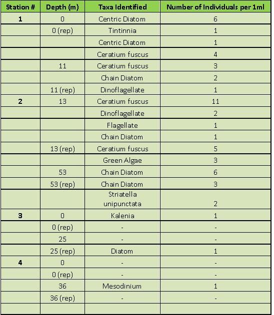 Figure 7.1: Table of Phytoplankton Species and Numbers
Figure 7.2: Zooplankton Species Offshore |
|||||||||||||||||||||||||||||||||||||||||||||||||||||||||||||
|
Chemical |
CLICK TO ENLARGE IMAGES |
|||||||||||||||||||||||||||||||||||||||||||||||||||||||||||||
|
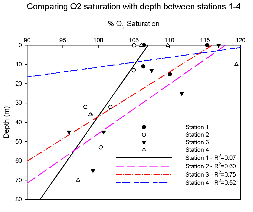
Dissolved Oxygen In all cases, oxygen saturation decreases from the surface, which is unsurprising given the nominal influence of photoautotrophic oxygen production. However, station 1 was the most well-mixed of the offshore series, showing the most homogenous oxygen % saturation with depth. Based on the temperature and salinity data for stations 1-3, the surface 20m of the water column shows super-saturation of oxygen. At station 4, the most stratified, a dramatic decline in O2 saturation is observed throughout the water column. Due to its position and proximity from land, station 4 is clear of the mixing front and is experiences minimal tidal mixing, inferring that wind is the dominant mixing source. Thus, the rapid fall in O2 saturation can be explained by poor surface mixing associated with reduced wind stress during the summer months. Stations 2 & 3 were surveyed to allow assessment of the differences between both sides of the mixing front. At these stations a relatively similar gradient of AOU was observed, with the more well-mixed station 2 having a slightly higher saturation throughout (2-5% greater than station 1). Nutrient Discussion Chemical analysis of the water samples, and the concentration profiles constructed from this processed data, showed several trends and contrasting features between stations. The nutrient profiles for all four offshore stations show an initial increase in concentration (nitrate and phosphate) with increasing depth. An exception was observed at station 2 where phosphate appears to decreases up to a depth of 13 metres. A nutrient maximum was observed at varying depths for each station, above which they have been utilised during the spring bloom and have not yet been replenished due to the stratification. In addition to this, the depth of this maximum increases offshore with overall water depth. The chlorophyll concentration initially increases with depth, until chlorophyll maximum is observed. The depth of the maximum varies with station. At station 1, the chlorophyll maxima is located at a depth of 15 metres whereas at station 4, the maximum is 20m deeper. The increase in chlorophyll concentration relates to the corresponding decrease in phosphate concentration at the same depth, visible in the first 30 metres of the water column at each station. This can be explained by the nutrient utilization by photoautotrophic organisms. Silicon values were relatively high with values ranging between 0.3 and 0.7 at the surface, and 1.8 and 2.0 at the silicon maximum for each station. This maximum may result from the presence of diatoms, although low numbers are generally observed during summer months due to phytoplankton succession. Surface nitrate values fall between 1 and 1.5 µM at all stations, increasing to an observed deep maximum of 3.25 µM at station 3 (at 65 metres). These low values can be explained by the preceding spring bloom which removes nutrients from the water column. Seasonal stratification prevents nutrient exchange between the deep waters and the nutrient deprived surface waters. These results reflect the typical structure of the local coastal region, post spring bloom, during the summer months when a strong thermocline forms and stratification occurs.
|
Figure 8.1: Oxygen Saturation with Depth
Figure 8.2: Station 1 Figure 8.3: Station 2 Nutrient Profile Nutrient Profile
Figure 8.4: Station 3 Figure 8.5: Station 4 Nutrient Profile Nutrient Profile
|
|||||||||||||||||||||||||||||||||||||||||||||||||||||||||||||
|
Physical |
CLICK TO ENLARGE IMAGES |
|||||||||||||||||||||||||||||||||||||||||||||||||||||||||||||
|
Velocity Direction, Magnitude and Backscatter Due to technical difficulties with the ADCP no data could be collected below 25m. This also prevented ADCP surveying between station 1 to station 2 on the outward journey, however it was possible to obtain data on the return journey. During transect 1 no data was recorded as the boat was moving too fast, this appeared as a blank section on the ADCP plot. Transect 1 Transect 1 was taken between station 2 and station 3 at 10.35 (GMT), 25 minutes before high water. The average direction of flow was northeast, corresponding to the flood tide moving into the English Channel. In the first horizontal 2000m, the direction of flow in the upper 13m was south-southwest, with velocity magnitude of approximately 0.075 m/s. As the survey progressed along the transect, the direction of flow moved northward and the velocity magnitude changed to approximately 0.2m/s. Below 13m depth, the direction of flow changes to an easterly flow (from northerly) and in the region centred around 4000m, turbulence can be observed. This is reflected in the variation of colours observed on the plot. Below 13m, the velocity magnitude changes from 0.2m/s (between 0-2300m along the horizontal) to 0.075m/s in the region of turbulence. Velocity magnitude then returned to approximately 0.2m/s for the remainder of the transect. The change in velocity direction from south-southwest to north could be associated with a tidal front. It is characteristic to find a high abundance of plankton at a front due to nutrients being mixed upwards into nutrient depleted upper waters. This is observed along transect 1, where a region of high backscatter indicates the presence of zooplankton which feed on the phytoplankton. Moving along the transect the intensity of the backscatter dissipates, reflecting a decline in abundance with increasing distance from the front. Transect 2 Transect 2 runs from station 3 to station 4, and began at 12.32 (GMT), approximately 1.5 hours after high water. In top 10m of water, eastward flow dominates. Below this depth, the dominant flow changes to a westward direction. The velocity magnitude varies from 0 to 0.3m/s both along the transect and vertically through ot the water column with no identifiable patterns. The backscatter along this transect is high at the surface due to wave action. Moving down through the water column there are shallow layers of high and low backscatter. Areas of high backscatter represent particles within the water column, for example photoautotrophic organisms. Transect 3 Transect 3 was carried out between station 2 & 1 and commenced at 15.20 (GMT), approximately 2 hours before low water. The average direction of flow was southwest, but below approximately 7 meters, the direction of flow is less uniform. This can be seen with the increasing frequency of red/pink/blue pixels amongst the common dominant green (South-westerly flow). This south-westerly direction corresponds to the ebb flow out of the English Channel. The pattern in velocity direction observed corresponds to the pattern seen with the change in velocity magnitude. At stations 1 & 2 the water column is well mixed, but as the transect progresses, there is a slight increase in stratification associated with a decrease in the bottom water temperature. In the shallow region (horizontal distance - 3500 to 6000m) there is an area of high back scatter at the surface, attributed to a high abundance of zooplankton. Moving further offshore, the intensity of the backscatter decreases and the region of highest backscatter deepens from the surface to 5-10m.
The same Ri calculation as used for the estuary data was applied to the offshore data. Station 1 For station 1, CTD values were collected down to an approximate depth of 13m. Values indicating stable waters were found between 6-7 and 8-11m. Shear flow instability was recorded between 1-3 m and the remainder of the water column was well mixed. Station 2 For station 2, CTD values were collected down to an approximate depth of 25m. Values indicating mixed waters were found between 2-3, 9-10, 12-18 and 19-24m. A value indicating shear flow instability was found between 4-6m. The rest of the values were higher than 1, thus suggesting the waters between these layers were stable. Station 3 For station 3, CTD values were again collected down to an approximate depth of 25m. The majority of the water column exhibited stable conditions although there were some layers of unstable waters. Between 3-5m and 9-10m waters were well mixed, and shear flow instability was found between 2-3 and 11-12m. Station 4 For station 4, CTD values were collected to an approximate depth of 25m. Waters were well mixed in the layers between 3-5 and 9-10m. Layers between 1-3 and 8-9m showed some shear flow instability, whilst the rest of the water column was stable. In conclusion, at stations 3 and 4 there is a layer of highly stable water between approximately 13-25m and 11-23m respectively, this relates well to the strong thermoclines observed at these depths. In contrast, for stations 1 and 2, the layers of stability found are largely a result of variation in velocity direction, rather than being induced by the presence of a thermocline. Vertical Stratification Coastal waters are generally areas of poor stratification, as surface and tidal mixing result in a well-mixed water column. Further offshore, the water column becomes affected by wind stress and tidal mixing begins to decrease. Stratification is therefore more likely to develop. A tidal mixing front is a boundary between well mixed waters on the landward side, and stratified offshore waters (summer-autumn). As solar radiation diminishes and storm intensity increases, stratification breaks down and nutrient concentrations are homogeneously distributed throughout the water column. A thermocline is a region within the water column where a rapid change in temperature occurs over a short range in depth. During the summer, a strong thermocline forms, above which wind stress is the dominant mixing force. Wind intensity rarely penetrates deep enough to disrupt the thermocline resulting in strong stratification. Furthest offshore (station 4), the thermocline amounted to a change of ~5oC over 8m. As a consequence of the rapid change in temperature, the salinity (calculated via conductivity, temperature & density) experiences a significant spike. This spike is a product of the lag between actual change in temperature, and the temperature recorded by the CTD (most pronounced at station 4, with a decrease of 0.84 salinity units). The spike disregarded, the salinity varies by <0.2 over the 70m profile, hence the spike represents a far out of range measurement which can only be explained by the temperature lag. The surface layer is characterised by low nutrients as they have been utilized during the spring phytoplankton bloom. Low chlorophyll concentration was also recorded representing low phytoplankton abundance associated with the fading bloom. As a consequence of the low nutrient content of surface water in summer, a deepwater chlorophyll maxima forms below the thermocline where tidal mixing sustains nutrient supply to a sufficient degree to support primary production. A 15m increase in the depth of the euphotic zone was observed between stations 2 and 4, providing sufficient light for phytoplankton growth deeper in the water column.
|
Figure 9.1: Velocity Direction at Transect 3
Figure 9.2: Velocity Direction Figure 9.3: Ship Track at Transect 1 at Transect 1
Figure 9.4: Velocity Direction Figure 9.5: Ship Track at Transect 2 at Transect 2
Figure 9.6: Ri Number Figure 9.7: Ri Number Station 1 Station 2
Figure 9.8: Ri Number Figure 9.9: Ri Number Station 3 Station 4
Figure 9.6: Station 1 Figure 9.7: Station 2 CTD Profile CTD Profile
Figure 9.8: Station 3 Figure 9.9: Station 4 CTD Profile CTD Profile
|
|||||||||||||||||||||||||||||||||||||||||||||||||||||||||||||
|
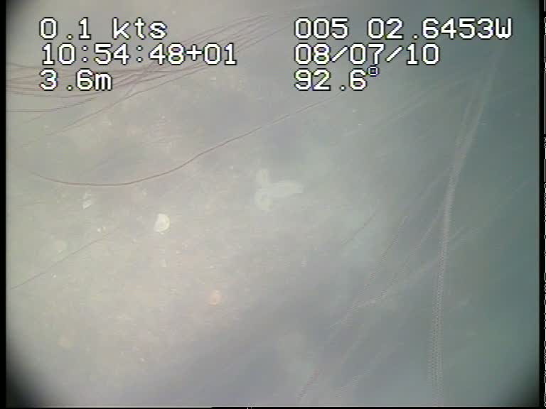
Introduction In 1992, the European Habitats Directive classified a 6387.8 ha area of the South-West Cornish coast as the ‘Fal and Helford Special Area of Conservation’ (SAC). The SAC aims to safeguard special features of the area including shallow inlets and bays, saltmarshes, intertidal mudflats and sub-tidal sandbanks. Protected Annex I habitats identified within the area include eelgrass meadows (Zostera marina) and the biggest maerl beds (Phymatolithon calcareum & Lithothamnion coralloides) in South West Britain. These benthic assemblages are important to the local ecosystem as they act as nursery grounds for juvenile fish and support a variety of rare organisms, including Couch’s goby (Gobius couchi). Benthic surveys of the area are therefore important in assessing long term change within the system. Aim On the 08/07/10, a benthic survey of the Fal estuary and Carrick Roads was carried out onboard SV Xplorer. The aim of the investigation was to map the habitat and the extent of the seagrass and maerl beds. Data collected was also made accessible to Natural England, allowing assessment of any changes in the coverage of benthic faunal assemblages. Method A GeoAcoustics Ltd dual frequency sidescan sonar was towed behind the vessel along a pre-determined track, at approximately 1m depth. A constant speed (4.4knts) was maintained as continuous data, relating to sediment type and topographic features, was collected. The instrument emits an acoustic pulse (“ping” rate of approximately 4 per second, at 415 kHz) from a towed “fish”, which is reflected by the seabed. The strength of the return signal received by the “fish” is dependent upon sediment type; more energy is absorbed by mud and silt leading to a lower return signal, whereas coarse sediments produce a higher return due to greater reflection. Four parallel transects were carried out, all approximately 100m apart. A swath of 150m allowed some overlap of adjacent transect.
|
||||||||||||||||||||||||||||||||||||||||||||||||
| Sidescan Sonar | ||||||||||||||||||||||||||||||||||||||||||||||||
|
Transect Locations and Times
Discussion and Analysis The sidescan sonar survey analysis revealed several artificial and natural features within the site of interest. The sediment changed from fine sediment in the North West of the surveyed sight, becoming coarser to the South East. This may be attributed to the increased energy environment of the deep channel, which cuts through the North bank. The Fal estuary is tidally dominated, producing varied bed forms highlighted on the sidescan trace. Sand waves and mega ripples are formed by diurnal tidal movements, and furrows are created by multi-directional estuarine currents. This accounts for the two perpendicular bed forms observed in the estuary. Areas of transverse ripples and dunes caused by currents can also be seen at the southern end of the study area. Three wrecks were detected, two of which were confirmed by local area charts; wreck (W1) was selected for further investigation using the submersible camera. She was identified by position as the SS Stanwood, which sank at its mooring on 10/12/1939 due to a failed attempt to extinguish a fire in the hold. The Stanwood was later destroyed with explosives to reduce the hazard posed by the feature, which would otherwise affect shipping movements. This explains the dissipated debris field located down into the channel identified on the sidescan trace.
Limitations Limitations of the side scan sonar are in the uncertain nature of the procedure. When analysing the printed side scan sheets one can only suggest what bedforms are on the sea bed. The side scan sonar provides an acoustic image of the sea bed not a photo. Therefore we could only infer what is there without actually knowing.
|
||||||||||||||||||||||||||||||||||||||||||||||||
| Van Veen Grab | ||||||||||||||||||||||||||||||||||||||||||||||||
|
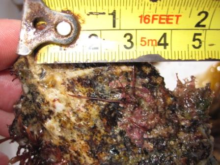
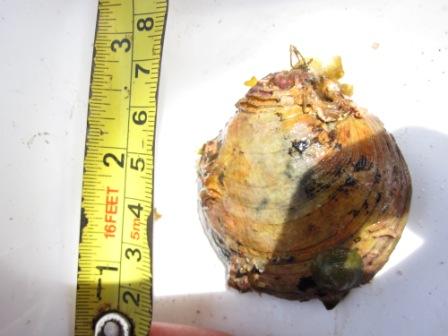
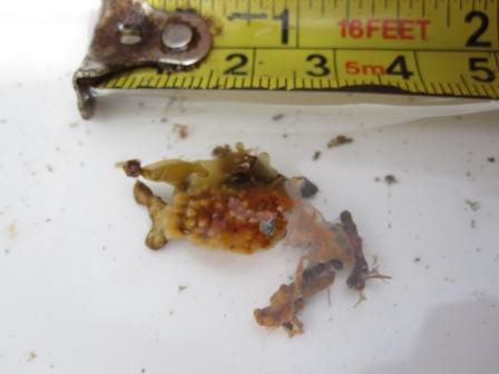
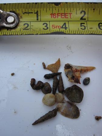
A Van Veen grab was used to sample specific areas of interest identified from the sidescan trace, and allowed ground truthing of the seabed type. Visual inspection of the benthos was carried out using a frame mounted video camera, preventing damage to the seagrass and maerl beds caused by the grab. The camera also allowed investigation of the shipwreck S.S. Stanwood, noted on the sidescan trace.
Figure 10.1: Polychaete Worm Figure 10.2: Bivalve Figure 10.3: Tunicate Figure 10.4: Gastropods |
||||||||||||||||||||||||||||||||||||||||||||||||
| Video Analysis | ||||||||||||||||||||||||||||||||||||||||||||||||
|
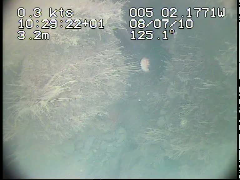
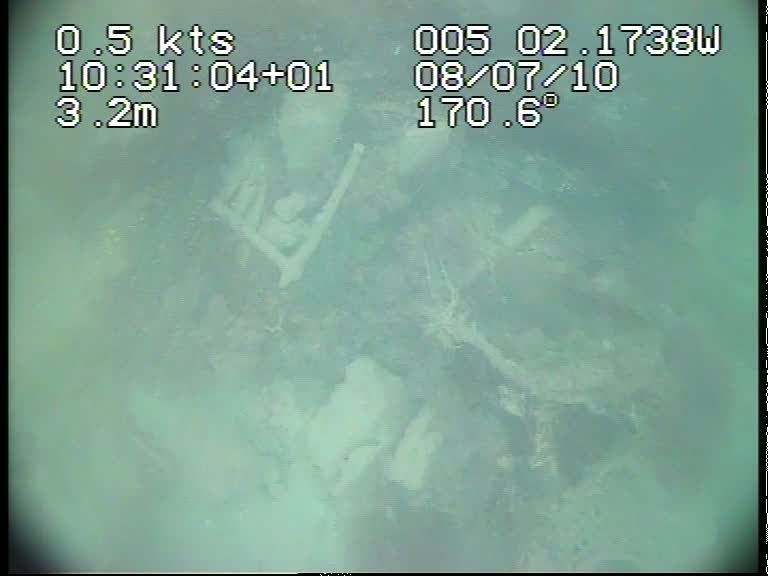
A video camera was deployed using the onboard winch system while the vessel drifted. This allowed visualisation of the benthic fauna, and identification of potential grab sites. The camera was deployed at 50°10.313N, 005°02.198W at 0917 (GMT) over the wreck of S.S. Stanwood, and was recovered at 50°10.322N, 005°02.156 at 0939 (GMT). Various algal species colonized the wreck allowing succession by fish and a diverse range of invertebrates, including bivalves and razor clams. The presence these organisms indicates that the wreck has become an important artificial reef ecosystem.
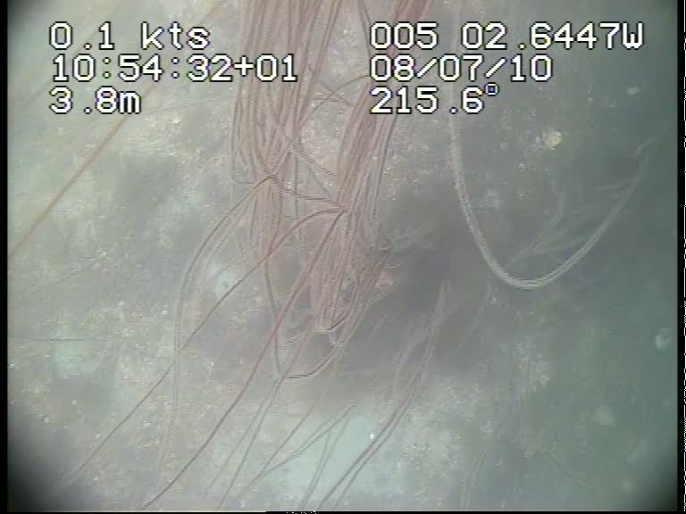
Figure 11.1: Video 1 Wreck Fauna Figure 11.2: Video 1 Wreck Fauna The camera was also deployed at 50°09.951N, 05°02.639 at 0954 (GMT) and was recovered at 50°09.955N, 05°02.636 at 09:57 (GMT). The seabed appeared to consist of muddy sand, maerl and broken shells. Asteroideans, bivalves, razor clams and red algae were observed in the benthos.
Figure 11.3: Video 2 Bed Fauna Figure 11.3: Video 2 Bed Fauna |
||||||||||||||||||||||||||||||||||||||||||||||||
| Conclusion | ||||||||||||||||||||||||||||||||||||||||||||||||
|
The sidescan plot interpretation showed the edge of the Carrick Roads channel sloping away from the west bank of the Fal estuary, further analysis allowed identification of typical estuarine sedimentary features as well as artificial components , in the form of three wrecks. Three sites were further investigated using the submersible video camera and, where possible, a Van Veen grab was deployed to investigate the biota. It was observed from these truthing methods that a number of different taxa and species have colonized the area. The wreck provides substrate for a number of different species of algae and has allowed a number of invertebrate and fish species to inhabit the area. The other area surveyed using video imaging and the grab showed that the sandy mud sediment also provides habitat for various algal species as well as invertebrates such as ascideans, molluscs and asteroideans. |
||||||||||||||||||||||||||||||||||||||||||||||||
|
During an 11 day fieldtrip to Falmouth, detailed measurements of coastal/ estuarine and offshore environments were undertaken. A variety of techniques were implemented, allowing investigation of the physical, chemical and biological parameters of the marine environment, local to Falmouth and the Western Approaches. Analysis of the Fal estuary revealed high salinities, and a low range throughout the estuary, due to low riverine inputs, the likely cause of which being low precipitation. High nutrient levels from anthropogenic inputs were also observed. An abundance of zooplankton was recorded, though phytoplankton numbers were very low. This was a result of strong autotrophic-heterotrophic coupling following the spring bloom. In contrast, the offshore data showed lower nutrient concentrations, decreasing with distance from the coast. Although phytoplankton abundance was greater than in the estuary, numbers were still relatively low following intense grazing and a decrease in surface nutrients, despite the increase in solar radiation. This was confirmed by the high numbers of zooplankton sampled offshore. A geophysical survey was conducted in Carrick Roads (the Fal estuary) in order to assess seabed features and benthic habitats. Sidescan sonar, submersible camera and a Van Veen grab were used to map the study site. Typical estuarine features were identified, along with three wrecks; one wreck, the SS Stanwood, and its associated fauna were visually inspected with the aid of the camera. Two grab sites were also selected; the fauna and sediment were logged. The grab sites were selcted following the sidescan analysis (and a video camera survey to prevent damage to fragile ecosystems such as Seagrass (Zostera marina). Estuarine sampling would have been repeated, to achieve a more representative dataset with a wider range of salinities; however this was not feasible due to time constraints and a shortage of suitable sample bottles. The offshore study was limited due to equipment malfunction, as the ADCP would not record data below a depth of 25 metres, thus restricting full analysis of the water column. The CTD light data was also discarded due to inaccuracies. In addition, the 200µm plankton net was damaged during its penultimate haul. |
|
The ideas expressed in this website are those of the group and do not reflect those of the University of Southampton or the National Oceanography Centre (NOC). |
![]()
![]()
![]()
![]()
![]()
![]()
![]()
![]()
![]()
|
Fofonoff and Millard (1983). "Algorithms for compilation of fundamental properties of seawater". UNESCO Technical Paper, Marine Sciences, vol 44, 53. Grasshoff, K., K. Kremling, and M. Ehrhardt. (1999). "Methods of seawater analysis". 3rd ed. Wiley-VCH. Johnson K. and Petty R.L.(1983) “Determination of nitrate and nitrite in seawater by flow injection analysis”. Limnology and Oceanography 28 1260-1266. Knauss, J.A., (1997). "Introduction to Physical Oceanography". Waveland Press. Langston, W.J., Chesman, D.S., Burt, G. R., Hawkins, S.J., Readman, J., and Worsfold, P. (2003), "The Characterisation of European Marine Sites. The Fal and Helford", JMBA, vol 8. Parsons T. R. Maita Y. and Lalli C. (1984) “ A manual of chemical and biological methods for seawater analysis” 173 p. Pergamon. Pingree, R.D. & Griffiths, D.K., 1978. "Tidal fronts on shelf seas around the British Isle". J. Geophys. Res. 83, 4615-4622. Miller C.B. (2004) "Biological Oceanography". Blackwell science. |