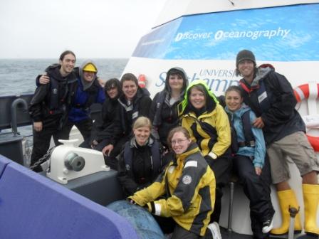
Introduction
Falmouth is situated on the south coast of Cornwall named after the river Fal (http://www.discoverfalmouth.co.uk). The coast is crucial for the areas economy by attracting
tourists due to a vast range of activities such as fishing,
farming and ship building (Howard et al., 2003).
The Fal estuary is considered to be one of the largest natural harbours in
the world, i.e. Carrick Roads (Langston et al., 2006). The
estuary has been described as macrotidal at the mouth, but has
been observed to be mesotidal further up-river towards Truro.
The wetlands on the upper part of Fal estuary are important
marine habitats which support rich flora and fauna communities,
but have been also subject to contamination by polymetallic
mining activity (Pirrie et al., 2003). After a major pollution
event during 1992, i.e. Wheal Jane incident (Younger, 2002), the
estuaries wetlands were characterised as
Special Areas of Conservation (SACs) (Langston et al., 2006).
Due to the important environmental features and the
contamination issues, Falmouth has attracted the interest of the
scientific community creating a long list of relevant research.
The aim of our survey is to provide additional information on
the Fal estuary and surrounding waters and to consolidate our
findings with existing data.
|
Equipment |
|
CTD
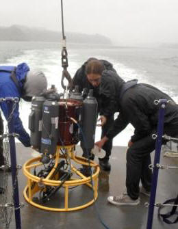 CTD
is an acronym for Conductivity, Temperature and
Depth. It measures distribution and variation of
water temperature, salinity and density. A CTD is
often attached to a rosette and lowered to the
surface via a cable. Another cable is attached to a
computer on board the ship and the CTD so it can be
controlled by the computer. Samples are taken at
regular intervals over a range of known depths.
CTDs are often very accurate but each small probe
has to be calibrated individually. CTDs are often
associated with Niskin bottles attached to the
rosette which collect water samples at wanted
depths. CTD
is an acronym for Conductivity, Temperature and
Depth. It measures distribution and variation of
water temperature, salinity and density. A CTD is
often attached to a rosette and lowered to the
surface via a cable. Another cable is attached to a
computer on board the ship and the CTD so it can be
controlled by the computer. Samples are taken at
regular intervals over a range of known depths.
CTDs are often very accurate but each small probe
has to be calibrated individually. CTDs are often
associated with Niskin bottles attached to the
rosette which collect water samples at wanted
depths. |
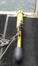
ADCP
 An
Acoustic Doppler Current Profiler, commonly
known as an ADCP, is an instrument used to measure
the speed of water through the water column.
It uses the principle of the Doppler Effect to
measure the speed of the water particles. The
device emits a series of high frequency ‘pings’ into
the water column which are scattered and reflected
by particles and the returning sound waves are
recorded by the ADCP. These returning waves
will have a different frequency to the original
emitted waves due to the Doppler Effect. If
particles are moving away from the instrument the
reflected sound waves return with a slightly lower
frequency. If the particles, however, are
moving towards the instrument then the returning
sound waves have a higher frequency. This
Doppler shift effect allows for the speed and
direction of a current to be calculated. ADCPs
emit four beams of sound, one pair measuring
E-W vertical velocity with the second pair
measuring north-south vertical velocity.
An ADCP can be left running to track the movement of
the ship and provide data on the bathymetry of the
sea bed. An
Acoustic Doppler Current Profiler, commonly
known as an ADCP, is an instrument used to measure
the speed of water through the water column.
It uses the principle of the Doppler Effect to
measure the speed of the water particles. The
device emits a series of high frequency ‘pings’ into
the water column which are scattered and reflected
by particles and the returning sound waves are
recorded by the ADCP. These returning waves
will have a different frequency to the original
emitted waves due to the Doppler Effect. If
particles are moving away from the instrument the
reflected sound waves return with a slightly lower
frequency. If the particles, however, are
moving towards the instrument then the returning
sound waves have a higher frequency. This
Doppler shift effect allows for the speed and
direction of a current to be calculated. ADCPs
emit four beams of sound, one pair measuring
E-W vertical velocity with the second pair
measuring north-south vertical velocity.
An ADCP can be left running to track the movement of
the ship and provide data on the bathymetry of the
sea bed. |
|
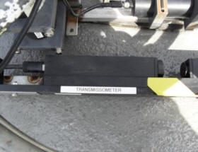
Transmissometer
A
transmissometer measures the turbidity of water by
measuring the fraction of light which reaches a light
detector at a set distance from the source. The
fraction of light, from the collimated source
reaching the detector is converted to the beam
attenuation coefficient (c). The light not reaching
the detector is due to absorption and scattering by
the water particles. The more light that reaches the
detector, the less turbid the water. The percentage
transmission is found from the following equation:
% transmission = (100%)e-cz
(where z is the length of the light beam)
|
Niskin Bottles
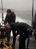 Niskin
bottles are used to take water samples at depth
without the issue of contamination. They are
often deployed on a hydroline made of reinforced
steel with a messenger weight. The bottle is
attached to the line and lowered into the water via
a winch system with both ends held open by rubber
bands or wire. A pressure sensor is usually
attached to the bottle as it is lowered as this
gives an accurate depth reading. When the
bottle reaches the sample depth the messenger weight is
dropped down the hydroline and hits the top of the
bottle. This collision disturbs the bands
holding the bottle open and therefore both ends
close. The bottle is then returned to the
surface. More than one Niskin bottle can be
used at once on one hydroline with the first
messenger creating a cascade effect of messenger
weights further down the line. If working in deeper
water a large number of Niskin bottles can be
attached to a rosette, often accompanied by a CTD.
They are held open by a number of pins which can be
remotely controlled from the vessel. This
allows for bottles to be closed at different depths
and if a large sample is required 3 or 4 bottles can
be closed in tandem. Niskin
bottles are used to take water samples at depth
without the issue of contamination. They are
often deployed on a hydroline made of reinforced
steel with a messenger weight. The bottle is
attached to the line and lowered into the water via
a winch system with both ends held open by rubber
bands or wire. A pressure sensor is usually
attached to the bottle as it is lowered as this
gives an accurate depth reading. When the
bottle reaches the sample depth the messenger weight is
dropped down the hydroline and hits the top of the
bottle. This collision disturbs the bands
holding the bottle open and therefore both ends
close. The bottle is then returned to the
surface. More than one Niskin bottle can be
used at once on one hydroline with the first
messenger creating a cascade effect of messenger
weights further down the line. If working in deeper
water a large number of Niskin bottles can be
attached to a rosette, often accompanied by a CTD.
They are held open by a number of pins which can be
remotely controlled from the vessel. This
allows for bottles to be closed at different depths
and if a large sample is required 3 or 4 bottles can
be closed in tandem.
|
|
Van Veen grab
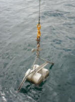 Collects
large samples of sediment through two grabs which
are clamped shut and returned to the surface. It is
operated on the ship. The amount of sediment in the
grab depends on the type of sediment being sampled.
Living organisms on the sea bed which are caught are
returned after observations. Collects
large samples of sediment through two grabs which
are clamped shut and returned to the surface. It is
operated on the ship. The amount of sediment in the
grab depends on the type of sediment being sampled.
Living organisms on the sea bed which are caught are
returned after observations. |
Secchi disk
 The
diameter of a secchi disk is between 20-30cm. It is
lowered into the ocean by a wire and the depth it is
lowered to is dependant on the operator. When the
secchi disk has disappeared from view then the
secchi disk length (Zs) can be
measured. The euphotic zone depth (Ze)
can be found by the following equation: Ze =
3Zs The
diameter of a secchi disk is between 20-30cm. It is
lowered into the ocean by a wire and the depth it is
lowered to is dependant on the operator. When the
secchi disk has disappeared from view then the
secchi disk length (Zs) can be
measured. The euphotic zone depth (Ze)
can be found by the following equation: Ze =
3Zs
|
|
Fluorometers
Fluorometers indicate chlorophyll levels in the
water so are therefore an indication of plankton.
They measure the amount of fluorescent radiation
produced by a sample exposed to monochromatic
radiation. Light is collected at a 90° angle from
the excitation direction. A photomultiplier tube is
often used as a detector.
 |
Plankton Nets
 There
are two types of plankton net that are used over the
course of the field trip, a vertical closing end net
and a bongo net. A vertical closing end net is
lowered into the water column and then slowly pulled
back up to the surface. A remote control is used to
close the net at a given depth. This allows
for specific sampling within a thermocline for
example. It has a diameter of 60cm and a 200μm
mesh. A bongo net is trawled behind the ship for a
short period of time just below the surface and
consists of two separate nets attached to one
another. Both nets have a 60cm diameter but
have different mesh sizes. There is a coarser
200μm net and a finer 100μm net. There
are two types of plankton net that are used over the
course of the field trip, a vertical closing end net
and a bongo net. A vertical closing end net is
lowered into the water column and then slowly pulled
back up to the surface. A remote control is used to
close the net at a given depth. This allows
for specific sampling within a thermocline for
example. It has a diameter of 60cm and a 200μm
mesh. A bongo net is trawled behind the ship for a
short period of time just below the surface and
consists of two separate nets attached to one
another. Both nets have a 60cm diameter but
have different mesh sizes. There is a coarser
200μm net and a finer 100μm net.
|
|
Side Scan Sonar
 This
instrument is used to identify the bathymetry of a
river or sea bed. A ‘tow fish’ is deployed
from a vessel and towed at around 8 knots. The
sonar beam hits the sea bed and reflects back to the
fish. The frequencies used in the majority of
side scan sonars range from 100 to 500 khz, with
higher frequencies providing a better resolution but
a smaller range. The sonar creates a black and
white image of the sea bed which can illustrate the
presence of bed forms, both natural and
anthropogenic. The image created can also
identify the type of sediment making up the sea bed
along the track as well as depth, height and width
of bed forms and even large shoals of fish. This
instrument is used to identify the bathymetry of a
river or sea bed. A ‘tow fish’ is deployed
from a vessel and towed at around 8 knots. The
sonar beam hits the sea bed and reflects back to the
fish. The frequencies used in the majority of
side scan sonars range from 100 to 500 khz, with
higher frequencies providing a better resolution but
a smaller range. The sonar creates a black and
white image of the sea bed which can illustrate the
presence of bed forms, both natural and
anthropogenic. The image created can also
identify the type of sediment making up the sea bed
along the track as well as depth, height and width
of bed forms and even large shoals of fish.
|
Sea-sickness tablets

Essential.
|
Analytical Methods
|
Silicon |
Analysed manually in
the lab using Parsons & Lalli (1984) method with a
Hitachi U1500 spectrophotometer at
810nm. |
| Phosphate |
Analysed manually in
the lab using Parsons & Lalli (1984) method with a
Hitachi U1800 spectrophotometer at
882nm. |
| Nitrate |
Samples were
analysed for nitrate content with a flow injection
method, Johnson & Petty (1983). |
| Dissolved Oxygen |
Grasshoff et al.
(1999) method, with particular care taken when
collecting and storing samples to avoid
contamination. |
| Chlorophyll a |
Two sources of
chlorophyll data were used in the Offshore and
Estuarine practicals. fluorometry values from the CTD
were converted to chlorophyll concentrations
to give a high-resolution vertical profile, and
samples from the Niskin bottles were also analysed
to support the CTD data, Parsons & Lalli (1984). |
| Phytoplankton |
Phytoplankton
samples were stained with Lugols solution and
settled overnight. They were then concentrated from
100ml to 10ml sub-samples for analysis under a light
microscope. |
| Zooplankton |
Zooplankton samples
were preserved using formalin overnight. Later, the
samples were inverted repeatedly to unsettle the
biomass from the bottom, and then 2ml was
transferred to a Bogorov cell for analysis under a
light microscope. |
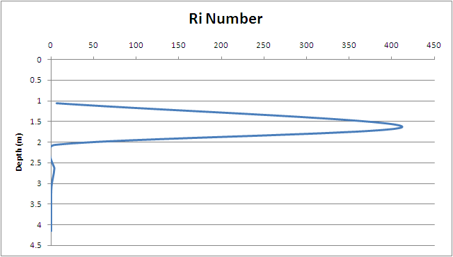
| Ri Number |
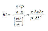 The
Richardson number (Ri) gives an indication as to
where mechanical mixing is likely to be taking place
in the water column and where stratification
prevents turbulence (Bob2010). When this number is
below 0.25 the water column can be said to be mixed,
and above 1 stable. Between the two there is a
transition stage. Ri is essentially the ratio of
stratification to the square of shear in the
horizontal current: The
Richardson number (Ri) gives an indication as to
where mechanical mixing is likely to be taking place
in the water column and where stratification
prevents turbulence (Bob2010). When this number is
below 0.25 the water column can be said to be mixed,
and above 1 stable. Between the two there is a
transition stage. Ri is essentially the ratio of
stratification to the square of shear in the
horizontal current: |
Back to top
Offshore Study
|
Aim |
Equipment |
Ancillary data |
Vessel Information |
|
To study how vertical mixing processes in the waters
off Falmouth affect, directly and indirectly, the
structure and functional properties of plankton
communities.
|
|
Date: 01/07/2010
Weather: Rain with 8/8
oktas
Tides: HW: 4.7m at 0805
GMT
LW: 1.9m at 1430 GMT
Sea State: Rough
|
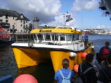
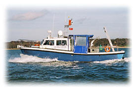
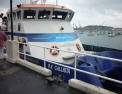 RV
Callista is largest of the three research
vessels used in Falmouth. It is 19.75m long
with a twin hull and a 1.80m draft. It has a
maximum cruising speed of about 15 knots and a range
of 400 nautical miles. Being a research vessel
it has a large A frame at the stern which has a 4
tonne capacity capable of deploying a CTD rosette
system as well as plankton nets and grabs. It has
two side mounted davits which have 100kg capacities.
The vessel can carry 30 passengers at one time as
well as a small crew of 3 and is equipped with both
wet and dry labs which contain microscopes and
computer monitors along with other sampling
equipment. This makes it an ideal vessel for sample
collection and analysis out on the water. RV
Callista is largest of the three research
vessels used in Falmouth. It is 19.75m long
with a twin hull and a 1.80m draft. It has a
maximum cruising speed of about 15 knots and a range
of 400 nautical miles. Being a research vessel
it has a large A frame at the stern which has a 4
tonne capacity capable of deploying a CTD rosette
system as well as plankton nets and grabs. It has
two side mounted davits which have 100kg capacities.
The vessel can carry 30 passengers at one time as
well as a small crew of 3 and is equipped with both
wet and dry labs which contain microscopes and
computer monitors along with other sampling
equipment. This makes it an ideal vessel for sample
collection and analysis out on the water. |
 |
|
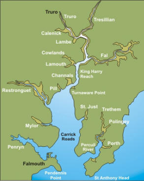
Google Earth
map of the six stations |
The importance of
vertical mixing on plankton communities is related to nutrients.
During summer, when nutrients are typically depleted in the surface
waters, the degree to which nutrients (esp. N and Si) can be cycled
up from depth is directly related to the abundance of phytoplankton
– the basis of all plankton communities.
Using the Callista
survey vessel and the equipment listed above, six discrete sites
were sampled along the coastal waters of the western English
Channel. Data from each site were
processed
in order to determine the amount of vertical mixing and
biological activity present, and then further
analyzed
to determine how the variables are related.
Each station was
initially sampled with a vertical CTD and ADCP profile, which were
then used to determine where, or if, water samples should be taken.
Niskin bottles were then fired at depth as the CTD ascended. These
samples were later analyzed in the lab for plankton abundance, as
well as nutrient content (N, P, Si), dissolved oxygen and
chlorophyll a.
| Station 1: Black Rock |
Time: 0828 GMT
Latitude: 50°08.053 N
Longitude: 005°01.524 W
Depth: 18.0m
Wind: 190°, 5.2m/s
Cloud Cover: 8 Oktas |
Results
|
Fig. 1a:
Nutrient profile
Fig. 1b: Oxygen
saturation depth profile |
The
water column at this station was relatively shallow,
with a depth of 18.0m. The CTD data showed that
temperature dropped by only 1oC
from 14.5°C at the surface (little or no thermocline)
and the salinity was constant at approximately 35.0
through the profile (see Fig. 1a). Fluorometer readings
indicate a maximum phytoplankton abundance between 5 and
10m, and the figure slightly decreases with depth below
this range. Both the nitrate and silicate concentrations
decreased with depth, with nitrate decreasing from
1.24μM to 1.09 μM and silicate decreasing from 1.13μM to
0.96μM down the profile (see Fig. 1a), however, only two
samples were taken, above and below the chlorophyll
maximum, so an expected peak may have been missed. The
phosphate concentration was uniform, with a
concentration of 0.01μM throughout the water column (see
Fig. 1a). No phytoplankton were observed in the samples
from this station under a light microscope, though it is
likely that they were too small or they weren’t stained
effectively by the Lugols solution. The fluorometry
readings indicate a chlorophyll maximum of 0.78µg/L at
10.0m (see Fig. 7d), which can be used to indicate
phytoplankton abundance. The Depth Average Chlorophyll
was 0.56µg/L. Zooplankton samples were taken from 14m
depth to the surface in a vertical profile. It was found
that the zooplankton community was dominated by the Copepoda, with an average frequency of 6881.31m-3
(see Fig. 8b). Aside from the Copepoda, the Cladocera
were the most abundant zooplankton group. Station 1
shows a nearly uniform distribution of oxygen with a
slight peak at 105.6% saturation, near the seabed at
15.6m (see Fig. 1b). This was a well mixed station so a euphotic depth of 21.3m is similar to what would be
expected for coastal waters, the chlorophyll
measurements from the fluorometer show a range of peaks,
with a maxima from 6-8 meters, and another smaller peak
at 18.0m, thus showing that light levels are sufficient
for photosynthesis to occur at 18m, which is consistent
with the calculated euphotic depth. The Attenuation
coefficient is again similar to the figure expected at
the mouth of an Estuary where a well mixed water column
with higher levels of suspended Particulate matter are
usually found, it is similar to station 6.
|
Fig. 1c: ADCP plot |
Discussion
Station 1
showed no significant thermocline or halocline, indicating a
well mixed water column which is expected of this station as
it was closer to the shore than other stations studied. The
results for chlorophyll indicate that the phytoplankton were
the least abundant at this station. Since lower nutrient
levels can be associated with higher phytoplankton levels at
other stations (Stations 2 and 5), it can be concluded that
zooplankton grazing is limiting the phytoplankton abundance,
since the Copepoda abundance was the second highest value
observed in this study at this station. The silicate and
nitrate concentrations decreased with depth, possibly due to
the deep chlorophyll maximum (between 5 and 10m). At this
station, our secchi disc and CTD data show that the light
levels are sufficient for photosynthesis at a depth of 18m,
which would tie in with the relatively deep chlorophyll
maxima that was observed.
| Station 2: The Bellows |
Time: 0950 GMT
Latitude: 50°11.114 N
Longitude: 004°47.967 W
Depth: 56m
Wind: 187°, 8.2m/s
Cloud Cover: 8 Oktas |
|
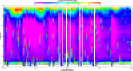
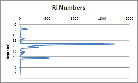
Fig. 2a: ADCP plot
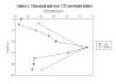
Fig. 2b:
Chlorophyll
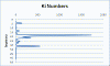
Fig. 2c:
Ri Numbers |
Results
The water
column depth at this station was 56.0m. Similar to Station 1
there was limited change in the salinity with depth. The
surface temperature was 14.6°C. There was a greater
difference in surface and bottom temperatures at this
station of approximately 2.5oC,
which could be due to deeper waters (see Fig. 2d). The
salinity increased from 33.3 at the surface to approximately
35.0 at 46.0m (see Fig. 2d). There is also a clearly defined fluorometry
reading maximum at this station than at others; the value increased
from 1.2 to over 2 volts in the first 25m of water. The nitrate
concentration decreased with depth, with a peak low value of 0.73µM
at 26.0m. The silicate concentration also decreased with depth,
with a peak low value of 0.64µM at 26.0m (see Fig. 2d). At
the first station only two Niskin bottles were fired so it
is hard to determine whether the nutrients recovered deeper
down. At this station however, the concentration of both of
these nutrients increases with increased depth. At this
station there was no change in the concentration of
phosphate which remained at 0.01μM (see Fig. 2d). No
phytoplankton were observed under a light microscope for
Station 2 samples. Fluorometry readings and analysis of
water samples were used to calculate chlorophyll
concentrations at this station. The fluorometry readings
follow a similar pattern to those of the water sample
calculations. The water sample chlorophyll concentrations
show a peak of 1.26µg/L at 26.0m (see Fig. 2b). The Depth
Average Chlorophyll was 0.69µg/L (see Table 2). Two vertical
profiles were conducted for zooplankton, one from 34m depth
and one from 20m depth. The Copepoda frequency was highest
at both stations, at 19469.03m-3 from 20m to the
surface. From 34m to the surface the Copepoda
frequency was lower, at 14177.94m-3 (see Fig.
8b).
Aside from the Copepoda, the Cladocera were the most
abundant zooplankton group in both samples. Station 2 shows
a defined oxygen saturation peak of 106.8% at 26.3m,
approximately halfway down the water column (see Fig. 2e).
The euphotic depth is 24.3, which is the deepest from all
the stations measured,
the water column at this site was
more stratified. There was a peak in chlorophyll just above
the bottom of the euphotic zone at 23m with a decrease in
chlorophyll present at deeper depths, indicating that the
euphotic zone does appear to finish around that depth.
The average Ri
at station 2 was 85.198, this is the highest value of the two
stations, showing there is less mechanical mixing throughout the
water column at this station. Fig. 2c shows a very stable
layer within the water column starting at around 17m; this is
consistent with fig 7b which shows a strong thermocline at around
10m. There is some mechanical mixing occurring at the surface,
likely due to wave action; with Ri values lower than 0.25.
|
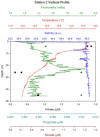
Fig. 2d: Nutrient
profile
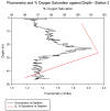
Fig. 2e: Oxygen
saturation depth profile |
Discussion
At Station 2 there was a well-defined thermocline and halocline,
indicating early stages of water column stratification as it
was relatively further offshore. Furthermore, the lowest
silicate and nitrate peaks were observed, which may be
limiting the phytoplankton abundance. The chlorophyll data
suggests the phytoplankton abundance was relatively low.
However, a major factor in the limited phytoplankton
abundance is the zooplankton, which far exceeded other
stations in terms of abundance, and were grazing on the
phytoplankton. The nitrate and silicate concentrations
decreased with depth, possibly due to the uptake of
nutrients by phytoplankton, which (according to the
chlorophyll maximum on the CTD data (See Fig. .)) are most
abundant fairly deep below the surface. The euphotic zone is
the deepest of all stations here, at 24.3m, which ties in
with the chlorophyll data which is at its maximum just above
this depth at 23m and starts to decline after this depth.
| Station 3: Off the Manacles |
Time: 1140 GMT
Latitude: 50°04.799 N
Longitude: 005°02.020 W
Depth 45.4m
Wind 200°, 7.5m/s
Cloud Cover: 8 Oktas |
|
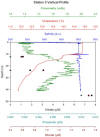
Fig. 3a: Nutrient
profile
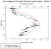
Fig. 3b: Oxygen
saturation depth profile |
Results The water column depth at this station
was 45.4m. The temperature decreased from 14.9°C at 1.0m to 11.9oC at 40.0m, but the salinity stays constant
at approximately 35.0 (see Fig 3a). At this station there is
a different pattern in the nutrient concentrations to the
two previous stations; the concentrations are at their
lowest at the surface. At this station the nutrients are
depleted in the surface 10m, but as with station 2, they
increase below the fluorometry reading maximum. Station 3
had the highest nitrate and silicate values of all stations;
nitrate increased with depth, reaching a peak of 7.65µM at
45.0m, and silicate peaked at 1.69μM at 45.0m (see Fig.3a),
also increasing with depth. Despite an increase in the
concentration, the phosphate value peaked at 0.01µM, as with
other stations (see Fig. 3a). Only two diatoms were counted
at this station, from a sample taken at 41m. Fluorometry
readings and analysis of water samples were used to
calculate chlorophyll concentrations at this station. The fluorometry readings follow a similar pattern to those of
the water sample calculations, but at noticeably different
concentrations. The water sample chlorophyll concentrations
show a peak of 0.86µg/L at 23.7m (see Fig 8a). The Depth
Average Chlorophyll was 0.87µg/L (see Table 8). We conducted
a horizontal zooplankton trawl at the near surface between
Stations 3 and 4 using a Bongo net, resulting in two
simultaneous samples, one of 100µm mesh size, and the other
of 200µm. Between Stations 3 and 4, the Copepoda frequency
was lowest, at 1589.26m-3 with the 100µm mesh and
1542.37m-3 with the 200µm mesh (see Fig. 8b),
however they still dominated the zooplankton community,
followed by the Cladocera. Station 3 shows a very well
defined oxygen saturation peak of 114.4% at 23.7m,
approximately halfway down the water column (see Fig 3b).
The current was too strong at this site for accurate secchi
disc data to be recorded.
|
Fig. 3c: ADCP plot
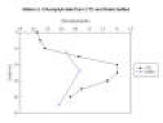
Fig. 3d:
Chlorophyll |
Discussion
At Station 3 there was no halocline but a
slight thermocline was present. Station 3 was more offshore so may
be experiencing slight stratification of the water column. The lack
of halocline may be due to the lack of influence of riverine input
compared with more inshore stations. Station 3 showed the highest
nitrate and silicate concentrations of all stations, and may account
for the fairly high depth average chlorophyll, and second highest
chlorophyll maximum (See Fig. 3d), indicating relatively high levels
of phytoplankton. Due to technical difficulties, no vertical
zooplankton profile was conducted, so the zooplankton cannot be
studied in relation with the phytoplankton. Nitrates and silicates
increased with depth, since below the chlorophyll maximum
approximately halfway down the water column, fewer phytoplankton
were taking up nutrients, however this would not explain the
increase between the surface and the chlorophyll maximum. This could
instead be explained by the production and downward flux of faecal
pellets and other organic matter containing nutrients into deeper
waters from the surface. It is also possible that the phytoplankton
are not nutrient limited, since the concentrations are exceptionally
high, and the nutrient distribution is determined by other factors,
although further study would be required to confirm this. The
relatively high dissolved oxygen content of the water column can be
attributed to the high phytoplankton abundance and activity,
producing waste oxygen.
| Station 4: Helmouth |
Time: 1246 GMT
Latitude: 50°05.825 N
Longitude: 005°03.995 W
Depth: 17.8m
Wind: 184°, 9.4m/s
Cloud Cover: 8 Oktas |
Fig. 4a: ADCP plot |
Results
The water column
depth at this station was 17.8m. As before, the salinity at
this station was constant. There is a temperature decrease
of approximately1oC over the entire water column
from 14.4°C at the surface, which is not as strong as in
stations 2 and 3 (see Fig. 4b). The salinity is approximately
35.0 throughout the water column. The nutrient profile for
station 4 is different from all other stations; after the
maximum reading from the fluorometer the concentration of
nitrate decreased with depth, with a low peak of 1.45 µM at
15.6m (see Fig. 4b), while silicate increased with depth,
with a peak value of 1.33µM at 15.6m (see Fig 4b).
Phosphate, again, was uniformly low at 0.01 µM and there was
no change with depth (see Fig 4b). No phytoplankton were
observed under a light microscope for Station 4 samples. The fluorometry readings indicate a chlorophyll maximum of
0.68µg/L at 10.0m (see Fig. 8a), which can be used to
indicate phytoplankton abundance. The Depth Average
Chlorophyll was 0.60µg/L (see Table 8). No zooplankton
samples were taken at station 4, instead a horizontal trawl
was conducted between stations 3 and 4. The
current was too strong at this site for accurate secchi disc
data to be recorded.
|
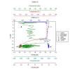
Fig. 4b: Nutrient
profile |
Discussion
There was no significant thermocline or
halocline at Station 4, indicating a well mixed water column
similar to other more inshore stations. There were
relatively few phytoplankton at this station; the
chlorophyll data shows this station had the lowest
chlorophyll maximum of all stations (near the seabed) and a
relatively low depth average chlorophyll value. The nitrate
concentration decreased with depth, probably due to uptake
by phytoplankton, and the silicate increased with depth.
This may be due to a relative lack of diatoms which utilize
silicate, so silicates are instead affected by abiotic
factors. No vertical zooplankton samples were taken, so it
cannot be confirmed that the low phytoplankton abundance is
caused by grazing, although this is a possibility.
| Station 5: Helford River |
Time: 1309 GMT
Latitude: 50°05.817 N
Longitude: 005°06.347 W
Depth: 5.8m
Wind: 192°, 3.8m/s
Cloud Cover: 8 Oktas |
|
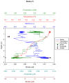
Fig. 5a: Nutrient
profile |
Results The water column
depth at this station was 5.8m. The water column was
slightly warmer than it was at station 4 (14.4°C at the near
surface), but the difference between the surface and bottom
temperatures is the same (1oC). The salinity
slightly increases from 34.9 at the surface to 35.0 at
5m(see Fig 5a). The nitrate and silicate profiles correspond
to the changes in salinity, while fluorometry readings and
phosphate concentrations correspond to the temperature
profile. The nitrate concentrations were low compared to
other stations and increased with depth, peaking at 0.78μM
at 5.2m (see Fig 5a). The bottom value of silicate on the
other hand, was the second highest out of all stations
(1.67μM) and increased with depth. Phosphate follows the
trend it set in the previous four stations; it falls below
detection levels at the bottom and the higher value is low
(0.01μM) (see Fig 5a). Three diatoms were counted in samples
taken from this station, from 1.47m depth. The fluorometry
readings indicate a chlorophyll maximum of 1.95µg/L at 1.0m
(see Fig 8a), which can be used to indicate phytoplankton
abundance. The Depth Average Chlorophyll was 1.78µg/L (see
Table 8). The chlorophyll concentrations at this station were
higher than that of other stations. No zooplankton
samples were taken at Station 5, since ADCP and CTD data
showed a relative lack of plankton abundance (See Fig 5b). The dissolved oxygen profile of Station 5 is not
uniform compared to Stations 1 and 4, with a peak of 107.9%
near the seabed at 5.2m; an increase of 2.8% from 1.5m. This site was very shallow, as it was into the
Helford Estuary, the euphotic zone continues to the sea bed.
The attenuation coefficient is higher than at the other
sights, at 0.36. This is most likely due to the increased
turbulence within the Estuary which was nearing the end of a
flood tide.
|
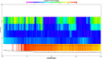
Fig. 5b: ADCP
plot |
Discussion
The Depth Average Chlorophyll was
highest at Station 5, indicating the highest phytoplankton
levels studied at these stations. No zooplankton samples
were taken, however ADCP data shows a relative lack of
zooplankton in the water column compared with other stations
(See Fig 5b), which could explain the relatively high
abundance of phytoplankton; there was limited grazing by
zooplankton. It can also be concluded that nitrate values
are the lowest at this station due to the high abundance of
phytoplankton. Both nitrate and silicate increased with
depth, which can be explained by the surface activity of
phytoplankton. The chlorophyll maximum is at 1.0m, so
nutrients are taken up at the surface and are thus depleted
compared with deeper waters, which have fewer phytoplankton.
There was no significant thermocline or halocline at this
station, indicating a well mixed water column. Unlike all
other stations, the dissolved oxygen does not correspond to
phytoplankton activity in the vertical profile of Station 5.
Instead the saturation peak is at the seabed. The euphotic
zone extends to the sea bed due to the shallowness of the
water, so potentially photosynthesis could happen throughout
the water column, providing a potential explanation for the
high oxygen levels near the sea bed.
| Station 6: Falmouth River |
Time: 1347 GMT
Latitude: 50°07.717 N
Longitude: 005°03.354 W
Depth: 17.1m
Wind: 188°, 6.8m/s
Cloud Cover: 8 Oktas |
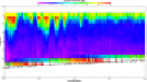
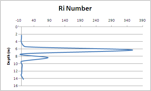
Fig. 6a: ADCP plot
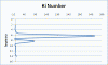
Fig. 6b: Ri
Numbers |
Results The water column
depth at this station was 17.1m. Station 6 was outside the
estuary, close to Black Rock (station 1) and this shows in
the salinity profile, which is back to being uniform. The
temperature decreases from 16.5°C at the surface to 14.3°C
at 12.5m (see Fig 6c). The thermocline is slight again, as
it has been for previous stations and the fluorometry
reading remains at similar levels through the profile. The
salinity increases from approximately 34.8 at the surface to
35.0 at 12.5m (see Fig 6c). The pattern for nitrate and
silicate is the same as it was at station 4, but the values
are reversed; nitrate increases from the surface to the
seabed (from 1.14 to 1.96μM) and silicate decreases (1.30 to
0.99μM) (see Fig 6c). The concentration of phosphate is
0.01μM for both sampled depths; staying constant through the
water column (see Fig 6c). No phytoplankton were observed
under a light microscope for Station 6 samples. The fluorometry readings indicate a chlorophyll maximum of
0.81µg/L at 6.0m (see Fig 8a) , which can be used to
indicate phytoplankton abundance. The Depth Average
Chlorophyll was 0.73µg/L (see Table 8). No zooplankton
samples were taken at station 6 due to time constraints. The
oxygen saturation at Station 6 shows a similar pattern to
that of Station 5, with a peak value of 109.2% approximately
5m above the seabed at 12.44m; an increase of 4.4% from 2.4m. Similar location to site 1, and has similar
attenuation coefficients and euphotic depth. Although the
water column is shallower at station 6 and it is very well
mixed, with no real peaks in chlorophyll. The euphotic zone
extends to the sea floor.
It is a well mixed
station with an average Richardson Number of 36.39;
this is lower than at station 2 indicating that it
is less well mixed. However is still considered to
have a very stable water column. Fig. 6b
shows a peak in the Ri number at around 6 meters,
which corresponds well with the slight thermocline
found at this station seen in Fig. 7b. At the
surface there is some mixing which is likely caused
by the wave action with an average value of 0.07 in
the first 4 meters thus below the Ri critical value
of 0.25. Fig. 6b also shows how stable the
water column is with very little change through out.
|
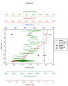
Fig. 6c: Nutrient
profile
|
Discussion
At Station 6 there was a slight
thermocline, but no halocline, indicating very slight
stratification as this station is slightly closer to the
shore than other stations with a slight thermocline. The
phytoplankton was reasonably abundant according to
chlorophyll data, with a shallow chlorophyll maximum
compared to Station 1, which was close to Station 6. This
corresponds to the increase of nitrate concentration with
depth, since uptake of nitrate occurs at a higher rate near
the chlorophyll maximum. The silicate concentration
decreases with depth. This may be because silicate is being
excreted rapidly by the plankton in the surface layers,
although further research would be required to confirm this.
No zooplankton data were collected for this station, so the
relationships between the plankton cannot be studied.
Vertical Profiles
 |
 |
 |
 |
|
Fig.
7a: Temp - Salinity |
Fig.
7b: Temp -
Depth
|
Fig.
7c: Salinity - Depth
|
Fig.
7d: Fluorometry -
Depth |
|
Chlorophyll
|
Depth
Average Chlorophyll |
Zooplankton |
 |
|
Stations |
(μg/L) |
|
1 |
0.56 |
|
2 |
0.69 |
|
3 |
0.87 |
|
4 |
0.60 |
|
5 |
1.80 |
|
6 |
0.73 |
|
 |
|
Fig.
8a: Chlorophyll - Depth for all Stations |
Table
8: Depth Average Chlorophyll for all Stations |
Fig.
8b: Zooplankton data for all Stations |
Summary
In summary, there are clear relationships between biotic,
abiotic and geographical factors along this area of the
south-east coast of the UK. The stations closest to the shore
tend to be well mixed compared to more offshore stations, due to
surface and seabed turbulence causing mixing, leading to more
thorough mixing of the water column in shallow waters. This
affects the temperature and salinity as has been shown in the
results and discussion. The phytoplankton at this time of year
are relatively low generally, as the typical Spring bloom has
passed, leading to depleted nutrients at depths which correspond
to phytoplankton activity (especially near the chlorophyll
maxima) and high numbers of zooplankton which feed on the
phytoplankton.
Back to top
Benthic Habitat Mapping
|
Aim |
Equipment |
Ancillary data |
Vessel Information |
|
To
effectively survey and categorize benthic habitats
in the Helford River using a range of geophysical
and biological techniques.
|
|
Date: 05/07/2010
Weather: Sunny with 2/8
cloud cover
Tides: HW 1100GMT, LW
1725GMT
Wind: 16knots average
Sea State: Calm
|
 SV
Xplorer: This vessel is ideal for both estuarine
and offshore work. At 12m long and with a 1.20m
draft it is able to navigate the mouth of a small
estuary much easier than the larger Callista.
It is also a much quicker vessel with a maximum
speed of 25 knots and a cruising speed of 18 knots.
It is equipped with a 1 tonne capacity winch on the
stern which is used for Van Veen Grab sampling. Side
scan sonar tow fish are also deployed from this
vessel. It can carry 14 passengers and the
wheelhouse can double up as a dry lab where the
progress of the side scan sonar can be monitored. SV
Xplorer: This vessel is ideal for both estuarine
and offshore work. At 12m long and with a 1.20m
draft it is able to navigate the mouth of a small
estuary much easier than the larger Callista.
It is also a much quicker vessel with a maximum
speed of 25 knots and a cruising speed of 18 knots.
It is equipped with a 1 tonne capacity winch on the
stern which is used for Van Veen Grab sampling. Side
scan sonar tow fish are also deployed from this
vessel. It can carry 14 passengers and the
wheelhouse can double up as a dry lab where the
progress of the side scan sonar can be monitored. |
Introduction
The Helford River is a
ria,
or a flooded river valley, fed by seven creeks. It
supports many types of industries, for example different
types of tourism and an oyster farm. Due to its
importance to people and the organisms living within its
environment, it has been a point of interest for both
conservation and development groups. The Helford River
is a Special Area of Conservation (SAC), a protected
site under the EU Habitats Directive and is home to many
rare species of marine life such as seahorses, gobies
and wrasse. It has gained status as a SAC due to
its various interesting habitats including mud flats,
sea inlets and sandbanks. These different habitats
support beds of the eelgrass, Zostera marina and
two species of the red calcareous algae maerl, L.
corallioides and P. calcareum, both of which
are protected species. The River incorporates the
National Seal Sanctuary which takes on injured seals and
nurses them back to health before later release back
into the Atlantic Ocean. This River is also a designated
Bass (Dicentrarchus labrax) nursery.
Two separate survey sites
were chosen for our study. One of these sites was
a known eelgrass area and it was chosen in order to
establish growth and abundance. Due to its status as a
protected species, it is important that such an area of
eelgrass is surveyed repeatedly. Eelgrass supports rich
invertebrate communities and lives submerged in seawater
in a range of habitat conditions and its survival is
subject to water clarity, sedimentation and various
forms of pollution (Langston et al., 2006). According to
relevant literature (Covey et al., 1987) it has been
observed that Zostera marina beds have
disappeared from many areas while the ones that remain
have been eroded. The effect of erosion on the eelgrass
beds is seen in this survey as the eelgrass abundance
was observed mainly in patches and not in extensive
eelgrass beds.
|
Images from video trawl |
 |
 |
|
Patchy Eelgrass |
More substantial Eelgrass Beds |
 |
|
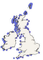
Maerl beds around the UK, sites
shown in blue. |
The
second site chosen was in the mouth of the
Helford estuary. This site was chosen as
it would hopefully provide a different benthic
habitat to that further up the estuary. It
was also presumed that this area would provide
grabs containing maerl. Maerl is a
collective term for a group of red algae that
form calcareous crusts on rocks, shells and
other substrates. They can form extensive beds
but are easily disturbed by changes in their
surrounding environment, including temperature,
salinity and heavy metal concentration of the
water column. The Maerl beds usually consist of
a mixture of two species of the algae, for
example L. corallioides and P.
calcareum. The exact combination of species
can vary with different environments. The
presence of Maerl beds has been a catalyst for
the introduction of new conservation sites
around the British Isles. This is due to it
being threatened by environmental and
anthropogenic pressures, such as the threat from
industrial use as it is often dredged and turned
into a powder for multiple used including a soil
conditioner and in water treatment. Maerl is
important in our ecosystems as it creates
habitats for smaller organisms which live in the
empty ‘shells’ of the Maerl, and it also affects
the substrate as it contributes to
biostabalisation on the sediment, making it more
coarse.
 |
|
Sidescan in Eelgrass beds, shown in
red
below |
 |
|
Sidescan in the Bay, shown in
blue
below |
At
both stations side scan sonar tracks were taken,
6 at the first site and only 2 at the second due
to time constraints. A drifting video
trawl was also undertaken at both, allowing for
a true view of the sea bed over which the tow
fish had just been dragged. Each time the
fish was being towed along a transect two
members of the group were positioned on the deck
as observers to note down anything that may
affect the sonar read out. The wake of
passing ships or the movement of moored buoys
could create cloud like trails on the print out.
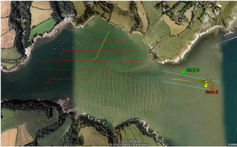
At the second site three grabs were performed
using a Van Veen Grab.
 |
|
Google Earth image of
benthic mapping transects |
|
Grab |
Location |
Time (GMT) |
Depth (m) |
Sediment type |
Organisms |
| 1 |
50°05.845N, 005°05.708W |
11:12 |
12.7 |
-
Medium – fine sand
-
Light brown
-
Uniform shape of sediment grains
|
- Live/ dead maerl
- Broken shells
- Unidentified
Amphipods
|
| 2 |
50°05.835N, 005°05.657W |
11:32
|
13.2 |
-
Medium – fine sand
-
Light brown
-
Uniform shape of sediment grains
-
Patch
of anoxic sediment
|
-
Large
shells, 3/4cm in size
-
Dead bivalves
-
Live
maerl
-
Bivalve - Donacidae
|
| 3 |
50°05.922N, 005° 05.907W |
11:52 |
12.1 |
-
Coarse/Mixed/Shingle sediment
- Larger rocks
|
-
Neriedae polychaetes
-
Hermit crab
-
Liocarcinus arcuatus
-
Ophiuroid brittle stars (Ophiothrix fragilis)
-
Brown algae
-
Bivalves
-
Amphipods
-
Janiridae isopod
|
Summary
By studying two separate sample
areas we are able to make a comparison between the variability
in the sea bed topography and its benthic habitats. Whereas the
transects in the mouth of the river showed a relatively
homogenous sea bed of medium sized sediment with patches of
fine, the other sample area further up the estuary produced a
sidescan track with a more variable sea bed. In this area there
were small areas of rock debris very close into the shore which
will have broken off the surrounding cliffs. Being this close to
the cliffs produces a unique habitat as it provides shelter and
a rocky substrate with plenty of crevices for organisms to live
and hide in. One area of our plot was hard to decipher as it
could have been either rock debris or yet another patch of sea
grass. Therefore it has been labelled as a mixture of the two as
it is impossible to determine without video analysis. The
majority of the rest of the sea bed at this site consists of
fine and medium sediment with an area of coarse sediment at the
eastern end of the transects. There were a lot less living
organisms further out into the bay than compared with in the
more sheltered part of the estuary where the video showed the
sea grass. This may be because they are more exposed to the
rough seas here. It may be that had we taken grabs closer to the
rock faces in the bay, we would have come across more biota, on
a more rocky sediment, more similar to further up the estuary.
The study area further up the estuary is a designated SAC site
due to the presence of protected eel grass meadows according to
the Joint Nature Conservation Committee. Using an ADCP and
sector scan we were able to determine areas in which sea grass
was growing. A video trawl was then undertaken to establish
whether the grasses were in a good state and the boundary was
discovered at 50°06.0150N, 005°06.6833W. We then saw a large
area of healthy sea grass close in to the shore, possibly
protected from the quicker currents present in the centre of the
estuary by a small headland. Sea grass grows best in slower
moving water and the ADCP data collected on the Xplorer backs
this up. Unfortunately, due to the constraints by the
conservation committee, we were not allowed to take grabs at the
sites of the sea grass so cannot be entirely sure what other
organisms are living in and around it, but it is possible for
wide varieties of sea life to flourish here; if more video
studies were conducted in this area we could inspect some of the
other life present. It is possible, due to the favourable
conditions in the estuary, the shelter from being close to the
rock face and the fact that researches cannot disturb them, that
a huge diversity of plant and animal life is present here, all
part of an intricate food web and ecosystem. It may be that
certain fish species use the sea grass beds themselves for
shelter and/or nursing grounds for their offspring. We also have
no idea, even using the video, of what organisms are living in
the sediments in this area, but they also play a huge role in
the ecosystem here as they affect the composition and structure
of the sediments.
Back to top
Estuarine Study
|
Aim |
Equipment |
Ancillary Data |
Vessel Information |
|
To study how the biological,
chemical and physical processes interact within the
Fal estuary |
|
Date: 09/07/10
Weather: Sunny, 2 Oktas
Tides: LW 0805 GMT,
HW
1415 GMT
Sea State: Calm
|
 The
Bill Conway is a smaller vessel than RV Callista
with a length of 11.34m and a beam of 3.96m. Its
full load draft is 1.4m making the Conway an ideal
vessel to navigate up small estuaries. It has an
average speed of around 10 knots which makes it
perfect for estuarine work. Two crew and twelve
scientists can be carried on the Bill Conway at any
one time allowing enough space for samples to be
collected. The A frame on the Bill Conway is 3m high
and its maximum capacity is 750kg which is ample for
any sample collected within an estuary. The trawl
winch is 70m which will reach the bottom of any
estuary enabling good samples to be obtained. The
Bill Conway is a smaller vessel than RV Callista
with a length of 11.34m and a beam of 3.96m. Its
full load draft is 1.4m making the Conway an ideal
vessel to navigate up small estuaries. It has an
average speed of around 10 knots which makes it
perfect for estuarine work. Two crew and twelve
scientists can be carried on the Bill Conway at any
one time allowing enough space for samples to be
collected. The A frame on the Bill Conway is 3m high
and its maximum capacity is 750kg which is ample for
any sample collected within an estuary. The trawl
winch is 70m which will reach the bottom of any
estuary enabling good samples to be obtained. |
 |
|
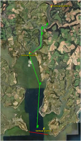
Google Earth map of transects and ship
track |
Estuaries
are bodies of semi-enclosed water that have different
biological, physical and chemical characteristics
compared to that of the seas into which they flow. They
form a transition zone between the fresh (riverine)
water environments and the ocean environments. The mix
of both the seawater and freshwater provide the water
column and sediment with a high nutrient concentration.
This alone makes the estuary one of the most productive
natural habitats in the world.
Wastes, transferring contaminants from heavily populated
or industrialised areas use estuaries as a convenient
channel to the coastal seas. Concentrated pollutants
tend to impact an estuary first due to the area being
more enclosed than coastal seas. Once the pollutants
reach the sea, processes in the estuary control the form
and concentrations of the various pollutants.
We took three ADCP transects (red lines) at
the mouth, middle and upper part of the
estuary to find the flushing time of the
estuary. At the same points we took
vertical
profiles of the water column to determine
the temperature, salinity and turbidity.
Ideally we would have measured fluorometry
but the fluorometer was not working.
However, samples for chlorophyll from the
Niskin bottles have been analysed in the
laboratory. The green line shows the five
points at which salinity decreased by 0.5
where we took nutrient samples to produce
mixing diagrams. The river-end member has
already been collected further upstream at 0
and 20.0
salinity.
It is
important to note that as the survey was undertaken
during a period of low rainfall, the salinity values
vary very little along most of the estuary. As
estuarine sampling is usually salinity-dependant,
this resulted in fairly low-resolution mixing
diagrams.
Depth Profiles
 |
 |
|
 |
|
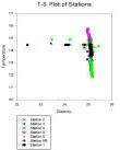
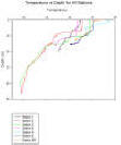
Fig.
1a: Temperature-Salinity plot |
Fig.
1b: Temperature -
Depth |
Fig.
1c: Salinity - Depth |
Fig.
1d Turbidity -
Depth |
Station
1 shows evidence of a slight thermocline (Fig. 1b),
over a few degrees as the measurements were taken
out in the mouth of the estuary. However, stations 2
and 3 were much shallower so a thermocline is not
present but temperature does decrease with depth. The
highest temperature recorded was at the surface at
Station 3 where there is least turbulence (Fig.
1b) and
the depth is shallowest. The highest turbidity was
at station 1 (Fig. 1d) which was constant throughout
the water column. Station 2 and 3 (Fig. 1c) show
salinity decreasing with depth whereas station 1 has
a constant salinity through the water column
representative of a well-mixed water column. The T-S
plot (Fig. 1a) also shows station 1 with a constant
salinity and only a small change in temperature
whereas stations 2 and 3 show larger decreases in
temperature and increases in salinity. Station 1 at
the mouth of the estuary has a light decrease in
temperature but is well-mixed. Further up the
estuary, with decreasing depth the surface is warmer
as less water to heat up and salinity is much higher
at depth as density increases.
The Richardson Number was calculated for Station
1 and 3, with an average of 11.82 and 2.68
respectively. This shows that at station one at
the mouth of the Falmouth Estuary is more stable
than further up the river, where ADCP data shows
that the current velocity is greater. The Ri was
calculated using un-calibrated salinity
measurements as the calibrated data was not
available at the time. This wouldn’t affect the
results as the change in shear stress would
still be detectable.
Station 1
|
 |
|
Fig. 2a: Nutrient depth
profile St. 1 |
Results
The first station sampled was a deep trough in
the middle of the mouth of the Fal estuary which
had a depth of 33m. Fig. 2a shows there
was a slight thermocline from 15.5ºC to 13.5ºC
but not much of a halocline with the salinity
staying relatively constant between 33.6 and 34.
The highest turbidity found during sampling was
4.397V (Fig. 1d) which was approximately
constant throughout the water column. The
nitrate minimum was 0.42μM at 4.4m whilst the
maximum of 1μM was observed at 20m. The
concentration decreases from the surface to 5m
then increasing down to 20m before decreasing
again at the bottom depth. The phosphate
concentrations show a decrease from the surface
to 5m then an increase. The maximum value for
phosphate was higher in the water column at
9.25m at 0.17μM. The results gave 0
concentrations at 19.8m and 25.7m. In the first
9.25m silicate has a completely opposite trend
to the two other nutrients with the
concentration increasing at 4.4m then decreasing
again. At 19.8m we see the maximum of 2.02μM.
This station shows an initial decrease in oxygen
saturation from the surface to 5 meters, and
then begins to increase; the biggest increase
taking place between 19.8 and 25.7 meters with
an increase of approximately 10%, resulting in
the highest oxygen saturation being 114.7% at
25.7m depth. (Fig. 7a) At Station 1 the
phytoplankton numbers were low. This was the
only station with Ceratum present and only
1,000,000 individuals could be found in 1m-3.
Dinoflagellates dominated the sample; the group
consisting of unidentified dinoflagellates,
Alexandrium sp., Karenia sp., and Gymnodinium
sp. (Fig. 5) The Copepooda dominated the
zooplankton community at Station 1, with
6375.52m-3, which is the lowest value of
Copepoda recorded for all the stations we looked
at. Appendicularia were abundant in the sample,
with 1499.31m-3. This is a very high value
compared to other stations and particularly to
that of the offshore samples (Fig. 6).
The chlorophyll data here is relatively low
compared to the other stations, not reaching
higher than 0.4746µg/L, and it is fairly uniform
as it only has a range of 0.3258µg/L (Fig. 7b).
The chlorophyll maximum is at the surface at
1.2m.
Discussion
The phytoplankton numbers here were the lowest
of all the stations visited, which may be tied
into the high turbidity observed, which would
restrict the amount of light available for
photosynthesis. The low chlorophyll levels at
this station support the hypothesis that there
are not many phytoplankton cells present here,
but we can assume that they are mostly in the
surface waters as the chlorophyll maximum is at
1.2m. The chlorophyll data are also relatively
constant throughout the water column which is
another indication of a mixed system. The low
abundance of phytoplankton may be the reason for
the low density of zooplankton found here, as
they would have little food to graze on. The
phosphate results are the highest at the surface
as they are being excreted by phytoplankton, and
the slowly decrease with depth as the
phytoplankton numbers decrease. There is an
anomalous reading where the concentration peaks
at about 10m depth; this could have been caused
by contamination of the sample. The Silicate has
an initial increase with depth, as the
phytoplankton abundance is decreasing and so
less silicate is being taken up. Below this
depth, the nutrients do not behave as would be
expected in this part of the estuary,
considering the results for factors such as
chlorophyll maxima and abiotic factors which
usually determine the nutrient levels throughout
the water column. These results can be explained
by pollution, as The Urban Wastewater Treatment
Directive has classified the Fal estuary as a
Sensitive Area (eutrophic) and the Nitrate
Directive designated the area as Polluted Water
due to eutrophication (Langston et al. 2006).
The initial decrease in oxygen saturation could
be due to the zooplankton which would be feeding
on the phytoplankton in the surface waters,
using the oxygen in respiration. The later
increase in oxygen could be due to the second
lesser increase in phytoplankton cells at around
20m which would reintroduce oxygen into the
water.
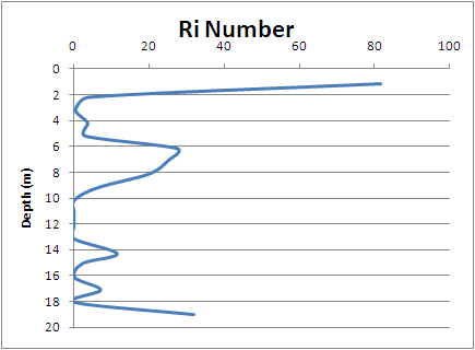
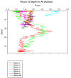
Fig. 8a shows the limited mechanical
mixing through out the water column, with some
mixing occurring at 10 to 12 meters. This
corresponds to the Brunt Vaisala frequency which
is lowest at that depth, but which also shows a
very stable water column.
Station 2
|
 |
|
Fig. 2b: Nutrient depth
profile St. 2 |
Results
At Station 2 the water temperature decreases
with depth from 16.51°C at the surface to
13.80°C at 15.3m depth. The salinity increases
with depth from 34.02 to 35.05. The
transmissometer reading increased from 4.10v to
4.26v, indicating increased turbidity at the
seabed compared to the surface. The nitrate
concentrations follow a strange pattern but this
time in reverse. At Station 2 the nitrate
maximum is at 3.18m (0.83 μM) and the minimum is
at 9.75m (0.17μM). The phosphate concentration
behaves in the same way as nitrate at station 1
with it decreasing at the surface but then
increasing again before decreasing near the sea
bed. The phosphate maximum was 0.26μM at 9.75m.
The silicate decreases very slowly from the
surface to 9.75m and then suddenly increasing
from 2.3μM to 9.0μM at 15.3m. Station 2 had
approximately the same number of total
phytoplankton m-3, 27000000, though a lower
diversity; only diatoms and Alexandrium sp. Were
present (Fig. 2b). The chlorophyll
maximum is 1.224µg/L, near the surface at 1.28m
(Fig. 7b). The zooplankton community at
Station 2 was composed almost exclusively of the
Copepoda, with a value of 159815.24m-3; the
copepods were very dense as well as very
dominant compared to other stations (Fig. 6).
The most abundant zooplankton after the Copepoda
were larvae of the Gastropoda with a frequency
of 392.61 m-3, however this value was very small
and did not deviate greatly from the frequency
of other organisms. Station 2 shows an initial
increase in oxygen saturation from the surface
to 3m and peaks here at 110.5%. After this, a
huge decrease of 13% occurs between 3.18m and
7.47m. It then gradually increases again as the
depth decreases (Fig. 7a).
Discussion
There is no thermocline but a halocline at
Station 2, probably due to its position in the
estuary. It is situated approximately in the
middle of the estuary between the sea and the
rivers, so the water column is likely to be
partially mixed with more freshwater overlying
more saline water. All nutrients are shown in
Fig. 2b to fluctuate between extreme values,
at depths which do not always correspond to
other factors such as chlorophyll maxima. This
can be explained by eutrophication and
pollution; The Urban Wastewater Treatment
Directive has classified the Fal estuary as a
Sensitive Area, and the Nitrate Directive have
designated the area as Polluted Water due to
eutrophication (Langston et al. 2006). The
oxygen saturation peaks near the chlorophyll
maximum, then decreases as the phytoplankton
abundance, indicated by chlorophyll
concentration, decreases. This is because
phytoplankton create large amounts of dissolved
oxygen at the surface. The turbidity is highest
near the seabed because increased friction
causes turbulence. The very high number and
density of the Copepoda can be explained by
eutrophication. It is possible that due to the
pollution of the estuary by nitrates and
phosphates a eutrophic event could have occurred
causing a large phytoplankton bloom. The
zooplankton would then have multiplied greatly
as they fed on the bloom, reducing the bloom to
more natural levels of phytoplankton in the
estuary, and resulting in a zooplankton
population explosion, where the Copepoda
outcompeted all other zooplankton Groups.
Station 3
|
 |
|
Fig. 2c: Nutrient depth
profile St. 3 |
Results
Fig. 2c
illustrates data collected right up the estuary
so one would expect to see low salinities and
high dissolved nutrient concentrations. It
could be argued that there is a slight
thermocline between 1.5 and 3.5m where the
temperature decrease 2ºC
from 18ºC
to 16ºC.
The salinity is incredibly high for the study
area, possibly due to lack of freshwater
inputs. The lowest salinity value was at the
surface, 31, with it increasing over the 5.25m
to 33.2. The turbidity increases from 3.96 to
4.14 at 2.87m before decreasing to 4.08. Here
the nutrient concentrations are at their
greatest. The nitrate maxima is at the surface
at 9.6μM
and it decreases linearly to 2.3μM
at 5.25m. The phosphate ranges from 0.59μM
to 0.27μM.
The silicate behaves in the same way as the
nitrate with the maxima at the surface at 8.4μM.
This is the only station at which the nutrients
have all followed a similar pattern and
decreased with depth.
Discussion
The plankton data (Fig. 5, Fig. 6) show
that this station was the most diverse; it had
the largest range of species for both
zooplankton and phytoplankton. Favourable
conditions encourage different phytoplankton
species to grow, which in turn promote
zooplankton growth by providing a range of
feeding niches. The chlorophyll maximum is at
the surface, showing that it reflects the number
of phytoplankton at this station. It is also the
highest of the chlorophyll maxima (Fig. 7b),
probably due to the conditions in the estuary.
Station 3 had the highest nutrient levels
and the maxima were at the surface (Fig. 2c).
This is good news for the plankton community,
but it could lead to eutrophication.
Eutrophication can lead to harmful algal blooms,
such as the red tide event of 1995-96, studied
by Langston et al. (2006). Our studies at
this station support this study; several species
of toxic phytoplankton where found such as
Alexandrium species and Karenia mikimotoi.
The CTD data show that there was a fair amount
of mixing going on, due to the combination of
shallow water and tidal mixing. Turbidity
increases with depth, which indicates that tidal
shear has more of an effect at 5m than at the
surface, however, the
euphotic zone extended to the bottom, allowing
phytoplankton to photosynthesise all the way
down.
At this station where the flow was greatest,
there is strong mixing seen near bottom of the
water column - likely due to the frictional
shear stress over the river bed. This can be
seen in Fig. 8b where Ri numbers are
around 0.0094, well below the mixing critical
value of 0.25. This data also corresponds well
with Fig. 1d, showing a high amount of
turbidity at around 3m depth.
Light data
 |
|
Fig. 3: Solar Irradiance - Depth |
Light will behave differently in
water to air. In water light is scattered and absorbed
by particles in the water column and is quickly
attenuated. The rate at which this occurs can be
quantified by the value k. K can be calculated in two
ways, using data from a secchi disk or alternatively
data from a light sensor. The formula for calculating k
using a secchi disk is very simple; k = 1.44/secchi disk
depth. This is however, not a very accurate form of
measuring the attenuation coefficient. Therefore one
can use the ratio between irradiance at depth (Ez) and
surface irradiance (Eo). The equation, Ez = Eo e-kz
can be rearranged to find k. This process is simplified
by creating a graph of Ln(Ez/Eo) against depth, finding
the equation of the line, and dividing 1 by the
gradient.
The
irradiance readings from the light sensor have allowed
for the construction of a graph illustrating the change
in solar irradiance with depth at each station. Fig.
3 shows that at all three of the stations the
irradiance decreases exponentially, with rapid decrease
in the surface layers and then a slow decrease at depth.
As one moves up the estuary the depth at which light can
penetrate decreases, due to increased particulate matter
in the water column. In just a metre the irradiance has
dropped from over 1000 at the surface to around 300μmol
m-2s-1 at station 3 whereas at
station 1 it is at 920μmol m-2s-1.
This illustrates how the surface layer of the estuary
will absorb or block a large amount of the incoming
solar radiation from reaching the water beneath. Fig.
3 shows how the irradiance figure at Station 1 does
not drop below 200μmol m-2s-1
until about 6m, whilst it occurs at much lower depths at
both Station 2 and 3. Station 2 appears to have the
sharpest decline due to the fact that the irradiance at
the surface was very high. However, it then follows a
very similar pattern to Station 1, ending a metre above
the sea bed with an irradiance of about 50μmol m-2s-1.
In accordance with the k values in Table 3, more
light is able to penetrate to greater depths at Station
1. A lower k value implies that less of the light is
scattered or absorbed by particles in the water column
and therefore the irradiance figures will be higher than
that of a station with a high k value.
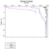
Table
3 also gives the depth of the euphotic zone, the
depth below which there is not sufficient light for
photosynthesis. This figure was calculated by
multiplying the secchi disk depth by 3. The euphotic
zone for Station 1 continues past the depth of the
profile in Fig. 3, but one can look at the amount
of radiation reaching the boundary at station 2 and 3.
At station 2 the boundary of the euphotic zone is 8.58m.
The photosynthetic active radiation figure at this depth
is 43.7μmol m-2s-1. The euphotic zone for
station 3 also
continues past the recorded depth of the light metre to
6.3m. This depth is within 10cm of the sea bed, implying
that phytoplankton would be able to photosynthesise
almost anywhere in the water column. Although 6.3m was
not recorded and one cannot definitely say that the
irradiance would be 40μmol m-2s-1 or less, it would be
foolish to suggest that the amount of light would
increase at this depth.
|
Station |
Secchi disk, k m-1 |
Ez/Eo k value, m-1 |
Euphotic Zone, m |
|
1
(50°08.659N,005°01.420W) |
0.238 |
0.211 |
18.15 |
|
2
(50°12.178N,005°02.429W) |
0.503 |
0.333 |
8.58 |
|
3
(50°14.395N,005°00.883W) |
0.686 |
0.630 |
6.3 |
Table 3:
Light data for all stations
Table 2 shows that the further
you travel up the estuary the greater the k value
becomes and therefore the euphotic zone decreases. The
euphotic zone will also decrease, however, due to the
decreasing water depth. At station 3 both k values are
within 0.06m-1 of each other. If the Ez/Eo
value is accepted as a truer value then k = 0.630
(3dp). Due to a smaller volume of water up the estuary
all of the absorptive material such as nutrients, SPM
and pollutants will be concentrated into a smaller area
and therefore the amount of light being scattered or
absorbed will greater. In contrast, the k value at
station 1 in the mouth of estuary was much lower at
0.211 (3dp), indicating that light will travel to much
greater depths through the water column. This is
because the volume of water is much larger here and the
scattering particles are dispersed throughout the
water. Station 2 is the only station which has k values
that are not within 0.1m-1 of one another.
This could be due to a change in the sunlight intensity
between the two measurement times. For example it could
have been very sunny when the secchi disk was deployed,
leading to inaccurate depth estimation and cloudy when
the light probe was used.
Estuarine Mixing Diagrams
 |
 |
 |
|
Fig. 4a: Nitrate Mixing Diagram - Removal |
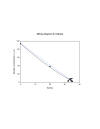
Fig. 4b: Phosphate Mixing Diagram - Addition |
Fig. 4c: Silicate Mixing Diagram - Removal |
-
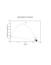
Nitrate mixing diagram (Fig. 4a) shows
non-conservative behavior of the constituent with
all the data bellow the theoretical dilution line
which suggests that nitrate was subject to removal
from the estuary. Most of nitrate removal was shown
at salinities 32 to 35.
-
Phosphate mixing diagram (Fig. 4b) showed the
strongest non-conservative behavior. Along the
estuary the concentration of phosphate was
increasing since the data points on the plot where
above the TDL. Most of phosphate addition took
place closer to the mouth of the estuary at
salinities 32 to 35.
-
Silicate mixing diagram (Fig. 4c) shows non
conservative behavior of the constituent with an
overall removal near the mouth of the estuary at
salinity 32 to 35.
The
nutrients, nitrate (NO3), phosphate (PO4),
silicate (Si) enter the open ocean through rivers via
estuaries, groundwater flow, and coastal zones.
Dissolved silicon is drained from land by natural
chemical weathering of silicate materials. The mean
concentration of dissolved Si in river water is much
higher than the concentration of NO3 and PO4
and within an estuary Si concentration decreases
towards the sea (Venucopalan et al., 2006). Si
concentration showed same pattern as suggested from the
relevant literature mentioned above i.e. the
concentration was decreasing towards the sea. Si is
also an important limiting nutrient for diatoms, thus
the removal can be accredited on the utilization of Si
by diatoms in the water column. Phytoplankton (diatoms
and dinoflagellates) were found during our survey up the
Fal estuary. The removal of nitrate, shown by the mixing
diagram, can be owed to the utilization by
phytoplankton. The strong non-conservative behavior of
phosphate can be attributed to anthropogenic input like
agriculture, sewage and other small inputs. In order for
the mixing diagrams to show a more reliable image of the
nutrients’ behavior in an estuary the amount of samples
collected for each nutrient must be around 50 or more,
over a range of salinities, as suggested by Head (1985).
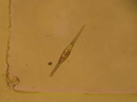 |
Phytoplankton |
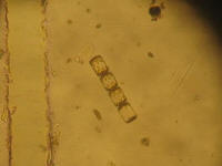 |
|
Ceratum fusus |
|
Diatom chain |
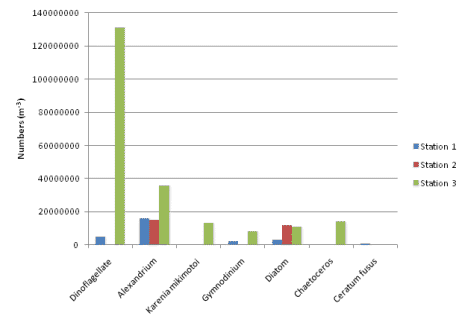
Fig 5:
Phytoplankton data for all stations
|
 |
 |
Zooplankton |
 |
 |
|
Hydromedusae |
Echinoderm larvae |
|
Copepod |
Mysidacea |
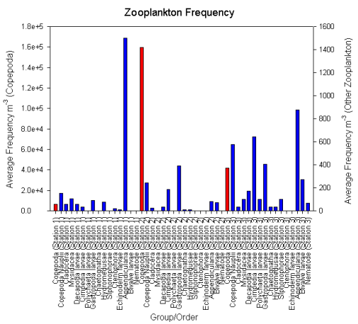
Fig 6:
Zooplankton data for all stations
|
Dissolved Oxygen
|
Chlorophyll
|
 |
 |
|
Fig 7a: Dissolved O2 for all
stations |
Fig 7b: Chlorophyll data for all stations |
|
Richardson numbers |
|
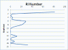 |
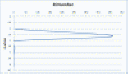 |
|
Fig 8a: Station 1 Ri Numbers |
Fig 8b: Station 3 Ri Numbers |
Summary
The biotic and abiotic factors of the stations studied
are expected of their position within the estuary; the
results for Station 1 show that of a well mixed water
column in terms of temperature and salinity, however the
nutrient profiles are not as expected due to pollution.
Station 2 shows similar nutrient profiles as a result of
this pollution. Station 2 is in between the sea and the
rivers entering the estuary, therefore it shows a
partially mixed water column. Station 3 appears not to
be as polluted as the other stations, resulting in
typical nutrient profiles, however this would have to be
confirmed by further research. Station 3 is atypical of
a river in terms of the water column; it is well mixed.
This can be attributed to the lack of freshwater input
due to limited rainfall, and the position of the tides
at the time of sampling.
Concluding statements
The offshore and
estuarine areas both displayed a great degree of
interaction between biological, chemical and
physical properties. The offshore showed that
the degree of mixing had a strong impact on the
abundance of plankton communities. A similar
pattern was seen in the estuary, where the
physics influenced the nutrients promoting
phytoplankton growth. The benthic mapping study
gave a clear, visual (through sidescan and video
data) representation of how the physical
processes affect benthic communities.
Back to top
References
Covey, R. &
Hocking, S., 1987. “Helford River Survey. Report for
the Heinz”, Guardians of the Countrysideand World
Wide Fund for Nature,pp 121.
Grasshoff, K.,
K. Kremling, and M. Ehrhardt. 1999. Methods of
seawater analysis. 3rd ed. Wiley-VCH.
Herdson
D. M., “The Helford river fish leaflet”, Helford
voluntary marine conservation area, pp 4
Howard P.,
Pinder D., 2003, “Cultural heritage and
sustainability in the coastal zone: experiences in
south west England”, Journal of cultural heritage,
vol: 4, p.p.:57-68.
Johnson K. and
Petty R.L.1983 “Determination of nitrate and
nitrite in seawater by flow injection analysis”.
Limnology and Oceanography, vol: 28, p.p.:
1260-1266.
Langston W.J.,
Chesman B.S., Burt G. R., Taylor M., Covey R.,
Cunningham N., Jonas P., Hawkins J. S., 2006,
“Characterisation of the European Marine Sites in
South West England: the Fal and Helford candidate
Special Area of Conservation (cSAC)”,
Marine Biodiversity,
vol:183, pp: 321-333.
Parsons T. R.
Maita Y. and Lalli C. (1984) “ A manual of chemical
and biological methods for seawater analysis” 173 p.
Pergamon.
Pirrie
D., Power R.M.,*, Rollinson G., Camm G. S., Hughes
H. S., Butcher R. A., Hughes P., 2003,“The spatial
distribution and source of arsenic, copper, tin and
zinc within the surface sediments of the Fal
Estuary, Cornwall, UK”, Sedimentology, vol:
50, p.p.; 579–595.
Younger, P.L.,
2002, “Mine water pollution from Kernow to
Kwazulu-Natal: geochemical remedial options and
their selection in practice”, Geoscience SW
England, vol:10, p.p.: 254–265.
Head
P. C., Practical estuarine chemistry, 1985,
Cambridge University Press, New York
Venugopalan
I., Unger D., Humborg C., Tac An N., 2006 ,The
Silicon Cycle: Human Perturbations and Impacts on
Aquatic Systems, Scientific Committee on Problems of
the Environment , USA. Wollast R., Chou L.
Disclaimer
The
views, opinions and scientific analyses
expressed in this website are those of the
authors and do not necessarily represent
those of the University of Southampton or
the National Oceanography Centre,
Southampton.
No animals were hurt in the duration of the
field course, other than a Seahorse and
several thousand plankton.
|