|

|
The
following methods were used to collect and analyse samples to ascertain
levels of chlorophyll, silicon, nitrate, phosphate and oxygen - methods
described below were relevant to both estuarine and offshore data. |
|
Chlorophyll - Sub samples (60ml) extracted from
the Niskin bottle samples collected by the CTD rosette system and
surface pump were filtered with the filters collected and placed in 6ml
of 90% acetone solutions over night in a fridge. The acetone solutions
having been left over night to dissolve chlorophyll from phytoplankton
collected on the filters were analysed for fluorescence levels to
determine amounts of chlorophyll and therefore relative phytoplankton
abundance. A calibrated flourometer with pure acetone(serial….) was
used to determine fluorescence of the samples (decanted into flourometer
cuvettes), normalized chlorophyll concentrations taking into account
volume of acetone (v) and media filtered (V) can be found by applying
the following equation with the flourometer reading (P, in µg/L): Chl.
In sample water = P x (v/V) |
|
Nitrate - Samples were collected at a number of
depths at known CTD stations using Niskin bottles mounted on a rosette
frame. Sub samples were filtered into glass bottles, left
overnight and refiltered to ensure no obstruction to the analytical
machinery. All vessels used were rinsed with a small amount of each
sample. 2-3 mL of sample was added to a system of flow-rated PVC tubes
with salt water and 2 reagents and through a catalyst of copperised
cadmium, converting nitrate to nitrite. Values for transmission for the
subsequent solution were measured and converted to millimetres using a
chart recorder.
The instrument used had a lower detection limit of 0.1µM |
|
Phosphate - Samples
were collected as for Nitrate above and prepared by the addition of 1ml
of a mixed reagent, bottles were then incubated for one hour to allow
colour to develop and a spectrophotometer was then used to determine
absorbance of light by the solution. A calibration graph created from
samples of known phosphate concentration was then used to determine the
phosphate concentration in the water samples. |
|
Silicon -
Again samples were collected as above and
subsequently prepared by pipetting 5ml of each sample into a tube and
adding 2ml of Molybdate reagent. After ten minutes 3ml of the mixed
reducing agent (MRR-metol sulphite, oxaic acid, sulphuric acid [50%v/v]
and milli Q water in the ratio 10:6:6:8 respectively) was added and the
solution left to stand for two hours for full colour development. A
spectrometer was used to determine absorbance of light by the solution.
A calibration graph created from samples of known Si concentration was
then used to determine the silicon content in the water samples. |
|
Oxygen - The Winkler method was utilized to
determine Oxygen Concentration as outlined by Grasshoff et al (1999).
The reagents added to the samples were 1ml manganese chloride and 1ml
alkaline iodide, in respective order. This was done immediately after
extraction from the Niskin bottles so to limit biological processes
within the sample bottles. Care was taken to ensure no air bubbles were
present in the sample bottles when inserting bottle stopper. Samples
were then stored and kept cool in a bucket of seawater.
|
|
Zooplankton Trawl - three trawls were carried out, 2 towed from the
Conway and a third from a pontoon as follows:
Table 1. Locations of zooplankton trawls
|
|
1 |
2 |
3 |
|
Start |
Lat:
50° 08.818N Long:
05° 01.518W |
Lat:
50° 10.316N Long:
05° 01.706W |
Lat:
50° 14.404N Long:
05° 01.878W |
|
Finish |
Lat:
50° 08.818N Long:
05° 01.630W |
Lat:
50° 10.402N Long:
05° 01.976W |
|
|
Meters Travelled Horizontally (M): |
47.1 |
176.7 |
2.4 |
|
Volume Of Water Filtered (M3): |
10.41562 |
39.07518 |
0.530732 |
|
|
Irradiance: A light meter was used to determine light attenuation in
the water and deployed at each of the CTD stations in the estuary, for
the offshore data a light meter was attached to the Rosette Frame. To
determine the light attenuation (k) at each depth the following equation
was used to determine the irradiance(ez) at each depth: Ez=eo-ekz
|
|
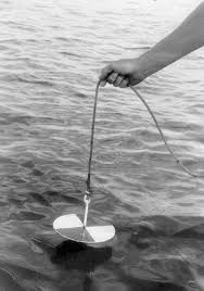
Secchi Disk
The light meter data were corroborated using
a secchi disk to monitor light attenuation at depth in both the estuary
and offshore at each of the stations at which the CTD was deployed. The
depth at which the secchi disk was no longer visible from the surface
was recorded and used to calculate the k value using the following
equation:
K (light attenuation)= |
|
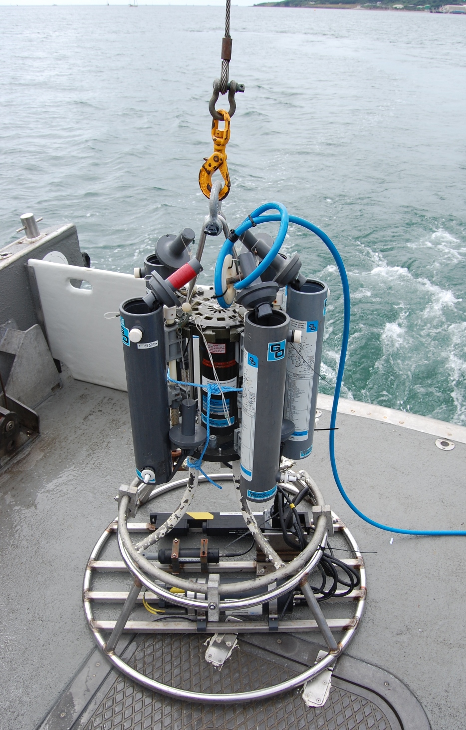
The CTD, measuring
temperature, conductivity (salinity) and depth, is attached to the
Rosette Frame with the
mid point of the Niskin Bottles being 65cm above the CTD for RV Bill
Conway and 1m for RV Callista hence all bottle sample measurements had
to be adjusted to reflect the actual sample depths. Also attached to
both Rosette Frames, at the same level as the CTD, were fluoremeters,
measuring fluorescence and transmissometers, measuring SPM (suspended
particulate matter) or turbidity. The RV Callista Rosette Frame also had
a light meter. Measurements from these instruments was recorded directly
to a computer programme and subsequently manipulated to provide the
results below.
|
|
ADCP
The ADCP
was used to conduct a number of transects during the estuarine study and
on a continuous basis during the offshore study. |


 |
|
INTRODUCTION
The aim of this study was to investigate the
interactions within the estuary between the chemistry, biology and
physics and to understand the horizontal and vertical changes within the
estuary characterised by the mixing properties of the freshwater and
seawater fronts.
Data were taken from
various stations along the estuary spanning from the mouth at Black Rock
(50o08. 444N, 5o01.098W) to the pontoon at King
Harry Reach (50o14. 444N, 5o00.834W), allowing for
a comparison of the behaviour horizontally up the estuary. Data
collection began in the morning of 30 June 2010.
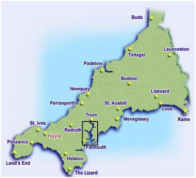
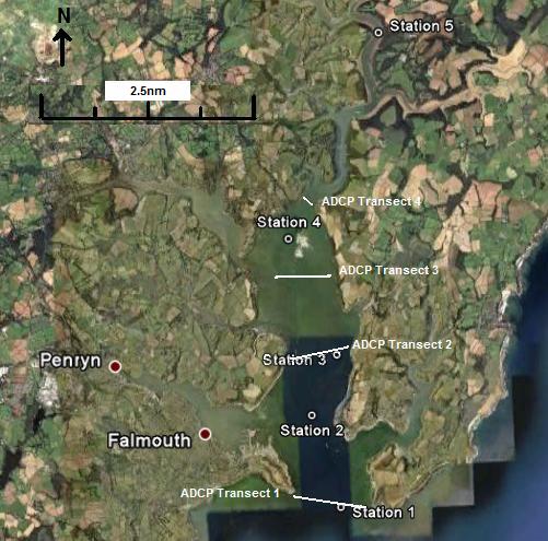
At 5
stations up the estuary (as marked on fig. 2.0) CTD profiles (mounted on
a rosette system with 5 Niskin bottles) were taken, with Niskin bottle
sample collection for nutrient analysis and data on fluorescence and
transmission taken from rosette mounted sensors; at 4 of these positions
ADCP transects were taken across the estuary to determine the physical
properties. At each station light meter readings were taken with depth
to determine light attenuation (k) values. The light meter data were
corroborated using a secchi disk whereby the depth at which the secchi
disk was no longer visible from the surface was recorded and used to
calculate the k value.
Due to
its Ria status, the estuary receives relatively small freshwater input,
so collection of freshwater end member samples was done an hour before
high tide on the 30/06/10 from Truro. This extra data will allow for
estuarine mixing diagrams to be made to study the behaviour of nutrients
in the estuary, along with the vertical profiles, light attenuation data
and data on plankton.
|
CTD
Data were collected at 5 stations, details of these stations, conditions
and tides were as follows:
Table 2 CTD station locations, weather and
tide information
|
CTD
Stations |
Lat |
Long |
|
|
Tide times |
|
|
 |
Figure 2.0 Map of CTD stations |
|
1 |
50°08.444' N |
5°01.574' W |
Wind speed |
4.9knots |
0149 |
Low |
1.2m |
|
2 |
50°09.605' N |
5°02.147' W |
Direction |
SW |
0723 |
High |
4.8m |
|
3 |
50°10.373' N |
5°01.656' W |
Sea state |
Slight |
1401 |
Low |
1.3m |
|
4 |
50°11.839' N |
5°02.611' W |
visibility |
good |
1930 |
High |
5.0m |
|
5 |
50°14.444' N |
5°00.834' W |
Cloud cover |
8/8 |
|
|
|
|
Four transects
were designed cross-sections of the lower, middle and upper
estuary at the following locations.
Table 3 ADCP transect locations |
|
ADCP Stations |
Lat/Long (START) |
Lat/Long (FINISH) |
Notes. |
|
Lower |
Transect 1 (East-West) |
50o08.440N 05o01.098W |
50o08.561N 05o02.495W |
8:32-8:48 GMT |
|
Transect 2 (East-West) |
50o10.417N 05o01.430W |
50o10.224N 05o02.646W |
10:30-10:43 GMT
At 338m, 020o alteration towards port. |
|
Middle |
Transect 3 (West-East) |
50o11.377N 05o01.805W |
50o11.339N 05o02.897W |
12:06-12:17 GMT |
|
Upper |
Transect 4 (East-West) |
50o12.267N 05o02.192W |
50o12.342N 05o02.299W |
14:12-14:16 GMT |
|
 |

Figure 2.0 Chlorophyll results |
Chlorophyll - at Station 1 chlorophyll concentration decreased
from the surface to 4m, then increased to a peak at 6m. After this peak,
the chlorophyll concentration remained constant with depth. The same
general pattern was repeated at Station 2, although both the minimal and
maximal peaks were deeper. This could indicate that the thermocline
deepened between Stations 1 and 2. Station 1at Black Rock is the most
seaward of the stations and marks the mouth of the Fal estuary.
Chlorophyll concentration in Station 3 shows an increase with depth, to
a maximum of 1.2uM at 4m followed by a sharp decrease to 0.9µM
at 8m and a further slight increase with depth. Station 4 shows a steady
chlorophyll concentration from surface to 2m, then a sharp increase
until a peak at 6m. Below 6m, the concentration remains relatively
constant. Station 5 shows a constant rate of decrease from surface to
4m. |

Figure 2.1 Nitrate results |
Nitrate: the
highest NO3 concentration (424.61µM)
can be found at the riverine end member,
likely to be due to the
introduction of anthropogenic inputs such as
sewage and agricultural run-off. Towards the
lower end of the estuary samples plot below the TDL indicating nitrate
is being lost from the system and behaving non conservatively. The
marine end member (35.07) has a concentration of 1.04uM
suggesting there is rapid removal of nitrate
from the estuary due to planktonic blooms, where nitrate is being used
as an essential element towards growth. |
Figure 2.2 Phosphate results |
Phosphate: the data
show that phosphate is acting conservatively in the estuary. One value
was discarded in order to produce the phosphate mixing diagram, which
was an anomalous result. This came from bottle 10 which was one of the
random samples from the onboard pump. This result was determined to be
an outlier, is still visible in the raw data but not included in the
final estuarine mixing diagram. |

Figure 2.3 Silicon results |
Silicon: Most plots lie
along the Theoretical Dilution Line showing that Si is conservative with
respect to the Fal estuary. This means that Si concentration is solely
dependant on mixing processes, and that there is no addition of removal
by any chemical or biological processes. |
|
Dissolved oxygen saturation has been plotted against temperature,
salinity and chlorophyll concentration for each station. Data have been
calibrated and depths have been corrected. Falmouth estuary is predominantly
saturated in dissolved oxygen with only the seabed at the riverine end of
the estuary showing under saturation. *Note samples were not taken at
station 4 due to sampling limitations, an ADCP profile only was taken. |

Figure 2.4 Station 1 Temp °C |
Station 1 shows a well
mixed water column at the estuary mouth, with salinity stable at 33.9 and
temperature range of 15°C at surface decreasing to 14°C at 15m depth where
it remains stable with depth. Dissolved oxygen saturation decreases
with depth to a minima of 100.3% at 15m, then increasing to a maxima of
104.7% at 20m. Chlorophyll increases with depth from 2.51μg/L at 4m to
7.27μg/L at 20m. |
 Figure
2.5 Station 2 Temp °C Figure
2.5 Station 2 Temp °C |
Station 2 shows a strong
thermocline at a depth of 2.3m, with a drop of temperature from 15.7°C at
surface to 14.7°C. Salinity increases from 31.9 at the surface to 35.3 at
depth. There is a dissolved oxygen saturation maxima of 107.1% at 5m, this
datum point is erroneous and could be due to machine error. Ignoring this
datum point, the general trend shows water column is oxygen enriched with a
lower saturation of 102.5% at surface increasing to 105.2% at 10m and 104.8%
at 20m. Chlorophyll concentration increases with depth except for a low at
5m, just below the diurnal thermocline. |
|
Figure 2.6 Station 3 Temp °C |
Station 3 shows
increasing salinity with depth, increasing from 33.4 at surface to 33.9,
with a halocline at approximately 5m. Temperature decreases with depth in
the mixed layer down to 10m, where temperature is stable with depth at
14.4°C. Oxygen saturation increases with depth down to 15m with saturation
of 105.7%, and decreases to 104.8% at 20m. Chlorophyll concentration follows
a similar trend with a surface value of 6.51μg\L increasing to 9.67μg/L at
8m and decreasing to 7.71μg/L at 20m. |

Figure 2.7 Station 5 Temp °C |
Station 5* the most
riverine station, was shallow with a sampled depth of 4.3m. Over this depth
salinity increases with a value of 31.1 at surface to 31.6 at 4m.
Temperature drops from a surface temperature of 20°C to 19.6°C at 4m. Only 2
water samples were collected, one at surface and one at 4m. Surface oxygen
saturation is the highest of all the stations with a saturation of 105.7%,
this drops to the lowest saturation level of all stations, with a saturation
of 98.7% at 4m. The chlorophyll concentrations are the highest of all the
stations with 107μg/L at surface dropping to 79.6μg/L at 4m. |
|
Zooplankton Trawl
Table 4 Zooplankton Trawl |
|
Tow Number |
Flowmeter Reading start (rotations) |
Flowmeter Reading end (rotations) |
Final Flowmeter Reading (rotations) |
Bottle Number |
Water Through Net in total tow time (m3) |
Figure 2.8 Zooplankton abundance |
The first two zooplankton tows were 5mins in
duration, the last 3mins as it was taken alongside a fixed floating
pontoon. |
|
1 |
12951 |
13108 |
157 |
B |
10.39 |
|
2 |
13109 |
13698 |
589 |
C |
38.91 |
|
3 |
13702 |
13710 |
8 |
A |
0.53 |
Overall
zooplankton abundance is much higher in tow 2 than any other tow; this
tow was carried out mid estuary, and for a length of 176meters, with 39m3
of water being filtered. Tow 1 then has the second highest overall
abundance. This tow was carried out at the mouth of the estuary; the tow
was 47m long, with 10m3 of water being filtered. Tow 3 was
carried out at the head of the estuary and displays the lowest overall
abundance.
Across the
species identified and quantified, a pattern can be seen in abundance
across the sites. Copepods have the highest abundance within all 3 tows,
being most abundant in tow 2, with 8675 copepods per m3.
Certain species were also only found at the seaward end of the estuary;
these species in particular are Ctenophores, Echinoderm larvae,
Appendicularia, Mollusca larvae and Siphoniphorae, with neither species
being found at the head of the estuary.
Horizontal distance (m) * area of net opening (m2) =
volume of water through net (m3). |
|
Phytoplankton trawl
The
phytoplankton counts have been conducted twice for each sample, except
for the one collected at station 2, for which a single count has been
made. The phytoplankton counts for all the samples range from 2 cells in
sample 1 to 24 in sample 3. 8 species have been recognised under
microscope analysis, with Karenia mikimotoi being identified at
all stations, while Alexandrium, Dinophysis and
Polytrictos have only been found in one over three stations.
Up to 16 Alexandrium
species of phytoplankton were identified on the first count in sample 3;
the occasional bloom of this type of phytoplankton is known as “red
tide”, and occurred for the first time in 1995 in the upper estuary, as
an indirect consequence of heavy metal pollution (Langston et al,
2003). The recurrence of Alexandrium in the sample collected at
the pontoon could be related to the same cause.
|
|
Table 5 Zooplankton Abundance |
Plankton Tow 1 |
Plankton Tow 2 |
Plankton Tow 3 |
|
|
N. in sample |
N. in sample |
N. in sample |
|
Groups/Order |
Count 1 |
Count 2 |
Count 1 |
Count 2 |
Count 1 |
Count 2 |
|
Karenia mikimotoi |
1 |
|
|
2 |
6 |
1 |
|
Guinardina flaccida |
|
|
|
2 |
1 |
1 |
|
Guinardina delicatala |
|
|
|
|
|
1 |
|
Mesodinium rubrum |
|
|
|
1 |
|
4 |
|
Alexandrium |
|
|
|
|
16 |
4 |
|
Dinophysis |
|
|
|
|
1 |
|
|
Polytrictos |
|
|
|
|
|
1 |
|
Dinoflagellates |
7 |
2 |
|
|
|
|
|
Total |
8 |
2 |
|
5 |
24 |
12 |
|
|
Irradiance |
|
Figure 2.9 Ez/Eo |
A graph showing the natural log of Ez/Eo
against depth was constructed (figure 2.10), the inverse gradient
of this line was used to determine k at each station.
The
light attenuation changes significantly with distance up the estuary
with the attenuation coefficient at station 5 from the light meter
reading almost an order of magnitude greater than that at station 1.
Irradiance: A graph showing the ratio of Ez/Eo
was constructed and displayed in figure 2.9.
Secchi disk results
show differences between the k values of the secchi disk and light metre
between stations have a range of 0.27m-1. |
Table 6 Comparison of Secchi disk and
light meter readings
|
Station |
k
m-1 (2d.p.) secchi disk |
k
m-1 (2d.p.) light meter |
|
1 |
0.21 |
0.20 |
|
2 |
0.32 |
0.25 |
|
3 |
0.37 |
0.26 |
|
4 |
0.46 |
0.44 |
|
5 |
1.13 |
1.51 |
|
Figure 2.10 Ln (Ez/Eo)
against depth |
Figure 2.11 Station temp profiles |
The highest surface temperature reading is at station
1 (20oc) due to the high volume of warm freshwater entering
near Truro. Water column temperature decreases downstream as it is
mixed with the colder water from Falmouth Bay. Below 2m, temperature
decreases by approximately 1oC for each station. |
Stations
1, 3 and 4 show little variability in salinity, with a range between
34.5 and 35.2. Station 2 has a lower salinity in the surface waters
(31.5) which decreases with depth below 1.5m. Station 5, has the lowest
salinity reading (31.1) as it is closest to the riverine input. Salinity
increases below 3m as the underlying saline water mixes with the
overlying fresh water. |
Figure 2.11a Station
salinity profiles |
Figure 2.12 Station fluorescence profiles |
Fluorescence is generally consistent with depth for
stations 1-4, with a small increase in values collected from stations
further upstream. Station 5 has a much greater fluorescence reading,
with a maximum value of 0.59v at 0.3m. |
Turbidity decreases with stations further upstream, although remains
consistent with depth. Station 1 has the highest turbidity reading
(4.47v) due to its proximity to the tidal influence at the marine end of
the estuary. Station 5 has the lowest turbidity reading (3.75v) although
increases to 3.9v at 5m |
Figure 2.12a Station
turbidity profiles |
|
ADCP |
|
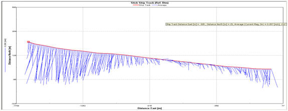
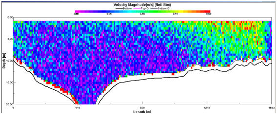
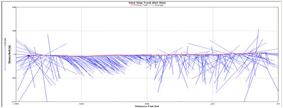
At the
lower estuary (Transect 1), the flow of the ebb tide shows a strong bias
towards the west bank of the estuary which is clearly shown by the Stick
Ship Track for Transect 1(Fig. 2.14). This circulation pattern is
present further up the estuary, shown by the Ship Stick Track for
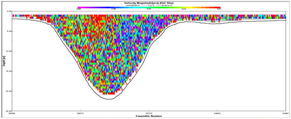
Transect 3 (Fig. 2.16). The Velocity Magnitude Profile for Transect 1
(Fig.2.15) illustrates that the area of high current energy is
restricted to the western bank and that there is a large area of low
energy present in the centre and east of the estuary. The Velocity
Magnitude Profile for Transect 3 (Fig.2.17) indicates that further up
the estuary the ebb flow, while still showing a bias for the west bank,
makes up a greater proportion of the water mass within the estuary. The
Ship Stick Track for Transect 3 (Fig. 2.16) and the Velocity Magnitude
Profile for Transect 3 (Fig.2.17) also illustrate that the net water
flow in depths of less than approx. 5m is retarded compared with the
unidirectional flow of the ebb-tide.
|
|
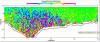
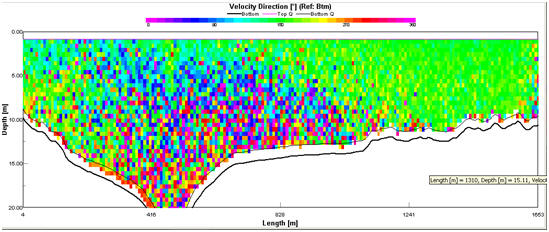
Figure 2.13 Velocity direction profile for
transect 1
|

Figure 2.14 Ship stick track for transect
1
|

Figure 2.15 Velocity magnitude profile for
transect 1
|
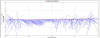
Figure 2.16 Ship stick track for transect
3
|
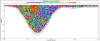
Figure 2.17 Velocity magnitude profile for
transect 3
|
|
Richardson Number:
The circulation pattern has important consequences for the Fal estuary.
The Velocity Magnitude Profile for Transect 1 (Fig. 2.15) and Velocity
Direction Profile for Transect 1 (Fig. 2.13) suggest that the ebb flow
moves on top of a stationary water mass generating two-layer flow in the
estuary. Two layer flow appeared to be present on the east bank of
Transect 2 and Transect 3 also. Using the UNESCO Equation of State
(1980) to covert the Temperature and Salinity readings from the nearest
CTD profile to density and the magnitude and direction of the flows from
the ADCP data, the Richardson number (Ri) was calculated to determine
whether the circulation pattern of the estuary enforces mechanical
mixing of the water mass specifically during an ebb tide.
The Ri numbers are all
below 1.0, suggesting that the water flow in the estuary is turbulent.
The Fal estuary is a combination of a fully mixed and partially mixed
estuary (Table 7).
The
circulation pattern also has important pollution and other consequences
for contaminants in the estuary. Any river source pollutants are going
to be restricted to the west bank of the estuary while the effects of
any marine source pollution will be concentrated on the eastern side.
The Ri number was then
plotted as a function of depth from the CTD profiles conducted at the
corresponding ADCP transect (fig 2.17). The plot of Ri profile of CTD
profile 1 for T1 (Fig. 2.17.T1.4) illustrates a laminar flow at the
surface <3m that changes to a turbulent/partially mixed water structure
>3m. It should be noted that the CTD profile data used to plot of Ri
profile of CTD profile 1 for T1 (Fig. 2.17.T1.4) was collected from
another group because of the anomalous readings collected by CTD profile
1. Further up the estuary the plot of Ri profile of CTD profile 2 for T2
(Fig. 2.17.T2.4) shows a reversed physical structure. The majority of
the water column, from the surface to 15m is partially mixed/turbulent .
Below this depth, layers of laminar flow are present and the plot of Ri
profile of CTD profile 3 for T3 (Fig. 2.17.T3.4) shows a similar
physical structure. At the furthest point up the estuary, the plot of Ri
profile of CTD Profile 5 for T4 (Fig. 2.17.T4.4) shows that the water
column is turbulent with a partially mixed layer along the estuary bed.
A recurring feature of the Fal estuary that the Ri plots have identified
is that physical structure of the water column alternates between
turbulent and partially mixed. Importantly, there no bottom boundary
turbulence layer in the estuary as might be expected. Fig.
2.17.T2.4-Fig. 2.17.T4.4 all clearly show bottom boundary induced
turbulence is suppressed by a laminar flow which is a characteristic of
partially mixed estuaries (Geyer, 1993). |
Table 7 Richardson numbers for Fal Estuary
ADCP transects
|
Transect |
CTD Profile |
Richardson number (Ri) |
|
1 |
1 |
0.07 Turbulent |
|
2 |
3 |
0.74 Partially mixed |
|
3 |
4 |
0.59 Partially mixed |
Figure 2.17 Profiles for Ri as a function
of depth for transects 1 to 4. (T1.4, T2.4, T3.4, T4.4) |
|
Fal Estuary Residence Time |
|
|

|
Smean = Mean Estuarine Salinity – Calculated from Stations
2,3,4 and 5 as equipment failure at station 1 prevented
correct results.
Ssea = Sea Salinity – Arbitrary figure of 35 used due to
equipment failure at station 1 prevented collection of true
marine end member
Vtotal = Total volume of estuary (m3), R =
Discharge rate of estuary (m3s-1) (Rough
estimation from Admiralty charts 5602.5 & 5602.3).
The rate of discharge of the estuary was calculated as a 10 year
average of July from 1999 – 2008 |
|
Year |
Rate of discharge for
July (m3s-1) |
|
1999 |
0.766 |
|
2000 |
0.988 |
|
2001 |
0.926 |
|
2002 |
1.006 |
|
2003 |
1.131 |
|
2004 |
0.678 |
|
2005 |
0.648 |
|
2006 |
0.586 |
|
2007 |
2.051 |
|
2008 |
1.948 |
|
AVERAGE |
1.074 |
|
NOTE: Data was collected from the Centre for Ecology and
Hydrology archives for the Fal station at Tregony. |
|
 =
687949.4s
Tres = 7.96 days
Due to naturally low rate of river discharge, the Fal estuary has a
long residence time. This has significant consequences as
pollutants from upstream tailings dams and sewage outfalls are
confined to the estuary for prolonged time periods. The recent
low precipitation levels mean that for 2010 the residence time
can be expected to be even longer, exacerbating the detrimental
effects of the upstream pollution inputs. |
|

The 5 depth profiles show a
slight decrease in salinity with distance up the estuary, this will be
because of a decrease in the saline member further up the estuary and an
increase in the freshwater member. Fig. 2.9-2.12 show the vertical
profiles of salinity, temperature, fluorescence and transmission at the
5 CTD stations within the estuary. The position of these stations is
noted in table 2. The fluorescence profiles show that stations 1-4 have
relatively similar levels of phytoplankton (remaining ~ 0.15-0.2v), with
some increase with distance up the estuary and decrease with depth at
station 4. Station 5 however shows much higher levels of fluorescence
(ranges between 0.4 – 0.6v), this may be down to the decreased size and
depth of the estuary at this point leading to increased nutrient
concentrations allowing for increased phytoplankton growth, this
apparent increase in fluorescence may also be helped by the decreased
amount of grazing zooplankton (see fig. 2.8).
Transmission:
decreases with distance up the estuary, ranging from 4.2 - 4.4v at
stations 1-4 to 3.8v at station 5, showing increased levels of
turbidity, this may be down to the shallow nature further up the estuary
leading to increased sediment suspension or simply may arise from the
increase organic input and phytoplankton at this point in the estuary;
it’s worth noting that these data agree with the secchi disk and light
meter data of greater light attenuation with depth further up the
estuary (see figs. 2.9 and 2.10).
Salinity: behaves in
a typical manor decreasing with distance up the estuary from the seaward
member, however with the small freshwater input the variation is small,
from ~35 at the stations in the main Carrick Roads channel (other than
the anomalous values from station 2) to ~31 at station 5. The station 1
data were taken from the 30/06/10 Callista data set as the Bill Conway
CTD initially gave clearly incorrect values (~19). The estuary seems
relatively well mixed as there is no sign of a strong halocline, other
than at station 2 which seems anomalous, however could be data from a
surface freshwater pocket.
Temperature: behaves
similarly but in inverse, with distinct differences with distance up the
estuary. The thermocline changes in depth, shallowing with distance up
the estuary as temperature increases. The thermocline seems a lot less
prominent at stations 4(4*)-5, with less than a 0.5oC change
with depth, as opposed to the 1-1.5oC change with depth at
stations 1-3.
The dominant force within
the estuary is tidal mixing, so where station 1 was taken at slack water
of the high tide, there was no mechanical mixing occurring allowing a
slight thermocline to form, as tidal currents increased throughout the
day and as data were collected further up the estuary the temperature
profiles show a more homogenous water column, with relatively little
fluctuation.
The CTD data show typical
partially/well mixed estuarine behaviour, with the values of components
as a function of tidal mixing and the meeting of seawater and freshwater
fronts.
|
|
Coriolis: From the data recorded by the ADCP, the ebb flow the
Fal estuary can be seen to be restricted to the western bank of Carrick
Roads. This corresponds with the circulation patterns of large bays and
enclosed seas in the Northern Hemisphere where the coriolis force
generated by the Earth’s rotation directs tides to circulate
anti-clockwise. It can be inferred that the flood tide of the Fal
estuary enters along the east bank and, while travelling up the estuary,
is restricted to the eastern side of Carrick Roads. The tide then turns
at the top of the large water mass above Transect 3 an the ebb tide
leaves along the western bank. At Transect 1 the ebb tide is forced into
the western English Channel. The ADCP Transects should be repeated on a
flood tide to confirm that this phenomenon is indeed present. However,
it should be noted that coriolis force is NOT the single determining
factor in terms of the circulation pattern of this estuary.
To see if the coriolis deflection could be
influencing the circulation of the estuary a simple equation can
constructed. Where a is the coriolis acceleration, t is
the length of time of the deflection. If result is greater than the
width of Carrick Roads the coriolis deflection is able to act for a long
enough time over a large enough distance to could be a contributing
factor to the circulation pattern of the estuary (width of Carrick Roads
approx. 1.7km).
a= fv = 10-4
x 0.5m
t2 = (2.16 x
104)2 = 4.67 x 10⁸s
 =
11.675 x10³m = 11km.
Coriolis can effect the tidal flow. =
11.675 x10³m = 11km.
Coriolis can effect the tidal flow.
The effect of coriolis is most likely balanced by a
pressure gradient across the estuary. The water on the eastern side of
Carrick Roads is a greater density than the water on the western side
because the highly saline seawater that enters the estuary on a flood
tide is restricted to the east bank whereas the low salinity freshwater
discharge is restricted to the western bank. This density difference
between the water on both sides of Carrick Roads forms a pressure
gradient across the estuary that balances the effect of the coriolis
deflection. Other factors, such friction, could balance the effect of
the coriolis deflection. |
The effect of coriolis is
most likely balanced by a pressure gradient across the estuary. The
water on the eastern side of Carrick Roads is a greater density than the
water on the western side because the highly saline seawater that enters
the estuary on a flood tide is restricted to the east bank whereas the
low salinity freshwater discharge is restricted to the western bank.
This density difference between the water on both sides of Carrick Roads
forms a pressure gradient across the estuary that balances the effect of
the coriolis deflection. 2 |


|
Introduction
The aim of this study was to
determine how the vertical profile of the water column changes at a set
offshore point over a 6 hour period. The time series data gained will
allow a study on the change in thermocline depth, and biological and
chemical activity with respect to this change throughout a tidal cycle.
Table 8:
Weather and Tidal data for 3 July 2010
|
Wind speed |
4.9knots |
|
Direction |
SW |
|
Sea state |
Slight |
|
visibility |
good |
|
Cloud cover |
3/4 |
|
0318 |
Low |
1.5m |
|
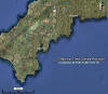 |
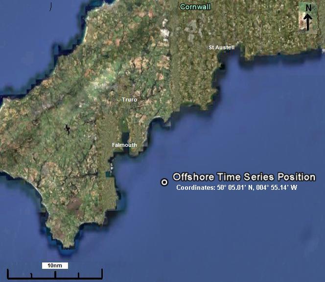
Figure 2.18 Location of offshore station |
|
0912 |
High |
4.5m |
|
|
1527 |
Low |
1.7m |
|
|
2117 |
High |
4.6m |
|
|
|
A time series of data
were taken over a 6 hour period on 3 July 2010 at (50. 05. 11 N, 4. 54. 95
W) to look at the structure of the vertical water column, phytoplankton and
zooplankton present at specific positions within the column. Vertical
profiles were taken using a rosette system with 5 Niskin bottles (see
methods) a fluorometer, transmissometer and CTD at 30 minute intervals
to a depth of ~60m. Surface to depth data were analysed to determine sample
collection points where changes were seen in the water column throughout a
tidal cycle. A continuous ADCP profile was taken allowing for judgment on
the changing zooplankton population and tidal flows beneath the vessel.
A continuous ADCP profile was taken allowing for judgement on changing
zooplankton population and tidal flows beneath the vessel. Data on tides and
weather was taken into account when choosing the station position, along
with an abundance of biological activity present; large number of diving
seabirds feeding indicated areas of food, in turn indicating fish abundance
and therefore high levels of phytoplankton. There was a moderate westerly
wind, with easterly tidal flow throughout the morning to one hour before
slack water at 1527 GMT. Niskin bottle samples were taken at profiles on the
hour, with zooplankton vertical tows taken at hourly intervals on the half
past profiles.
The transmissometer and ADCP are able to identify areas of higher SPM
(suspended particulate matter) indicating zooplankton or suspended sediment.
Using the data from the downward CTD profile the depth of zooplankton
sampling was determined from maxima in turbidity below the chlorophyll
maxima (that were inferred as being layers of zooplankton).
Ideally a closing zooplankton net would have been used, however this was
unavailable so was replaced by two vertical trawls, one beginning below the
maxima to surface, and one above to surface, so these abundance values could
be subtracted to find the approximate zooplankton abundance in the layer of
interest. A ‘bongo’ system was used, with a 100µm and 200µm mesh net.
Secchi disk depths to determine the euphotic depth at the station throughout
the day were also taken on the hour. |
|
For a
description of equipment used and analytical methods please follow the
 link.
link. |
 |
|
Chlorophyll:
The chlorophyll
results from all CTDs show a deep chlorophyll maximum in the morning,
shallowing towards the middle of the day and then deepening again in the
afternoon. In all CTDs sampled, the chlorophyll maxima equates to approx.
1.4μg/L. All three CTD profiles also show low levels of chlorophyll at the
surface. CTD1 shows a small chlorophyll peak at ~12m depth, which correlates
with nutrient graphs. After a small decrease, the main peak occurs at ~20m,
below which the chlorophyll decreases with depth. The second CTD shows that
the chlorophyll maxima has shallowed to ~15m and shows a very sharp decrease
with depth, but within a few metres the rate of decrease with depth slows
and the chlorophyll concentration continues to decrease until the end of the
profile, where an increase occurs. The third CTD shows a deeper chlorophyll
maximum than CTD2, and then follows the general trend of decreasing
chlorophyll with depth common to all the stations. |
Figure 3.1 CTD Chlorophyll profile |
|
Nitrate:
The data show that at the beginning of the day, the nitrate concentration
showed a clear minima at 12.23m, which correlates well with the chlorophyll
data. The general trend followed by the data is decreasing concentrations
from surface to the thermocline, with the minima being just above the
thermocline, then either increasing or remaining the same with depth below
the thermocline. |

Figure 3.2 Nitrate profile |
Phosphate:
The
graph indicates that phosphate concentration increases with depth. The
maximum phosphate concentration (0.31uM) recorded is found at 19.8m |
Figure 3.3 Phosphate profile |
|
Silicon:
The silicon concentration is plotted against depth for
stations 1,2 and 3. All transects show an increase in silicon concentration
with depth, ranging from values of 0.007 µM to about 0.011 µM, down to a
maximum depth of 50 meters at station 1. The rate of change of silicon
concentration with depth varies within each transect: at transect 1, the
silicon concentration remains approximately constant throughout the top 13
meters; it increases significantly between 13 and 24 meters, roughly
reflecting the thermocline, while below 24 meters the concentration
decreases linearly at a lower rate. The Si concentration trend at station 2
shows similar behavior to station 1, with a constant Si value throughout
the surface mixed layer down to 10 m depth, followed by a significant
increase at the thermocline (approximately between 10 m and 24 m), going
back to constant concentration below 24 m, reflecting a well mixed bottom
layer. The trend in transect 3 shows an increase in Si concentration with
depth from surface to 20 m depth. |
Figure 3.4 Silicon profile |
|
Oxygen: The percentage saturation of dissolved oxygen is highly
variable at the near surface waters ranging from 91-109% within the top 3
metres. There is then an area of high percentage saturation at around 10-20m
depth, though the range is still relatively large with values from 99 to
111% with no specific correlation between them. Percentage saturation
decreases sharply at 20-30m, just below the thermocline, with values of
82-85% saturation. After this the concentration increases slightly to around
91%at 31m and decreases steadily to 89% at 47m. |

Figure 3.5 Oxygen profile
|
|
Temperature: Throughout the day the defined
thermocline shallows dramatically (fig. 2.1) from ~25oC at
0840GMT to 18oC at 1330GMT, the temperature change in the water
column remains relatively constant, so the data have been displayed as
relative thermocline shape, with the values of each respective profile +1oC
of the previous. Surface waters remained at ~16.4oC, changing to
~11.7oC at the thermocline. |

Figure 3.6 Time Series temp profile |
|
Zooplankton tow: The
offshore zooplankton data were inconclusive, with clear errors that may have
arisen from the different methods to evaluate the depths of the tow nets.
The first tow was with a weight, with the second tow without and the rest
was with a depth meter so the actual depths of the tows are unknown and in
some cases negative values for zooplankton numbers were found at depths with
low transmission (high turbidity) readings. This data set does show however
the taxas present even if the depth of the tows and zooplankton maximas and
abundance per unit volume cannot be determined. As with the estuary, the
offshore water column was dominated by copepods, with much higher numbers of
Hydromedusae jellyfish. There was seemingly less Cirripedia larvae, but
similar amounts of copepod nauplii, Appendicularians and Cladocera. |
|
Turbidity:
Turbidity levels in the surface 10m are constistent with depth for all 4 CTD
stations, with a small decrease around 10m. The turbidity for all 4 stations
then increases to above the surface levels, at between 16 and 24m depth. The
turbidity falls between 25 and 27m, increasing again to another peak between
29 and 44m. In CTD3 this peak is not so sharply evident as in the other
profiles, and the eventual peak is delayed to below 40m. Below 44m the
turbidity decreases roughly linearly with depth to a minimum at the bed in
all profiles apart from CTD3, which shows high turbidity at the bed. |
Figure 3.7 Turbidity profile |
|
Fluorescence:
The general trend followed by the fluorescence data are of low surface
fluorescence, increasing to a peak roughly corresponding to the depth of the
1% surface PAR depth, then a decrease with depth below this. 1% surface PAR
marks the bottom of the euphotic zone, where the most common wavelength of
light is visible blue light. Red light is attenuated in the surface μm layer
whilst blue light persists to the bottom of the euphotic zone. CTD3
shows a main fluorescence peak around 20m and a smaller peak between 40m and
50m depth, which then sharply decreases again to follow the trend. CTD4
shows a main peak in fluorescence at between 15 and 20m, and another smaller
peak just below 60m. CTD4 also shows the highest surface fluorescence,
possibly as this CTD was taken at 1330 GMT when the surface PAR was
greatest.
|
Figure 3.8
irradiance profile |
|
ADCP
A continuous
ADCP was run for the duration of the time series (5hrs 16mins) to establish
the physical properties of the water column. This enabled the investigation
of any correlation between the changes in the hydrodynamic conditions on the
variation of a number of parameters (Temperature, Salinity, Chlorophyll,
etc.) that were measured over the course of the time series by comparing
the ADCP data with CTD data sets that were taken at the same times during
the time series. The continuous ADCP data were then separated into 5 data
sets: A1, A2, A3, A4 and A5:
Table 9: ADCP transect information
|
ADCP Data Set |
Time Start (GMT) |
Time End (GMT) |
Latitude |
Longitude |
CTD Profiles |
|
A1 |
08:55 |
10:04 |
50o05.023 N |
04o55.085 W |
1/2/3 |
|
A2 |
10:04 |
11:12 |
50o05.111 N |
04o54.945 W |
4/5 |
|
A3 |
11:12 |
12:11 |
50o05.109 N |
04o54.945 W |
6/7 |
|
A4 |
12:11 |
13:11 |
50o05.109 N |
04o54.941 W |
8/9 |
|
A5 |
13:11 |
14:11 |
50o05.123 N |
04o54.941 W |
10 |
At the start
of the time series the A1 Data Set shows that the water column is clearly
stratified.The Velocity Magnitude Profile of A1 (Fig. 3.9.A1.1) and Velocity
Direction Profile of A1 (Fig 3.9.A1.2) illustrates that the water column has
a clearly defined physical structure. Above 20m the water column oscillates
vertically as internal waves; gravity waves that oscillate within the water
column rather than at the surface. Internal gravity waves are common
phenomena in offshore coastal regions (Helfrich and Melville, 1986) and have
a significant role in the hydrodynamic properties of the water column,
increasing the mixing and transport components (Klymak and Moum, 2003). For
example, upwards transport of nutrients from depths into the euphotic zone
without disruption of the thermocline. The source of the internal waves is
likely to be the river plume of the Fal estuary as river plumes have been
identified as a source of large-amplitude internal waves in coastal seas.
(Nash and Moum, 2005).
Internal
waves propagate along layers of different density in the water column and in
A1 the oscillation is confined to a layer of reduced density above 20m. This
indicates the presence of a thermocline at 20m.
The profile
of the Backscatter Contour Profile of A1 (Fig. 3.9.A1.3) supports this
conclusion. Fig. 3.9.A1.3 shows a high level of backscatter in the top
layer down to a depth 20m, below which there is little reflectance . The
presence of a thermocline at 20m would explain this phenomenon. Dense
populations of zooplankton in euphotic zone cause the high levels of
reflectance recorded by the ADCP and as such, a chlorophyll max measured by
the CTD would be expected at this depth. The presence of phytoplankton
indicates the euphotic zone, the bottom limit of which is limited by the
depth of the thermocline.
To quantify
the physical structure of the water column for the A1 Data Set the Ri number
was calculated a function of depth for the CTD profiles that were conducted
between 08:55 and 10:04 average velocity recorded at each depth from the
ADCP (Fig.3.9.A1.1). The plot of the Ri profiles for each of the
corresponding CTD profiles for A1 (Fig. 4.0.A1.4) clearly shows the
structure of the water column. The thermocline is laminar flow that is
present at around 20m that separates layers of turbulent to partially mixed
water dynamics. This is analogous with data collected from each of the CTD
profiles 1, 2 and 3 that the water column is clearly stratified.
Importantly, Fig. 4.0.A1.4 shows the continuous vertical oscillation of the
thermocline over the course of the time series due to the oscillation of the
internal wave.
To determine
the strength of the stratification the Brunt-Vaisala Frequency was
calculated and plotted as a function of depth (Fig. 4.1.A1.5). The Brunt-Vaisala
Frequency is the maximum frequency that the internal wave can oscillate and
the results conclude that the stratification is stable.
The next
section of the time series was recorded by data set A1. In this data set the
physical structure of the water columned remained very similar. The Velocity
Magnitude Profile of A2 (Fig. 3.9.A2.1) and the Velocity Direction Profile
of A2 (Fig 3.9.A2.2) clearly show the presence of the internal wave is
restricted to the layer above the thermocline, suggesting that an upper
layer and a deep layer of greater density is present. The profile of the
Backscatter Contour Profile of A2 (Fig. 3.9.A2.3) illustrates that the upper
layer corresponds with the limits of the euphotic zone, suggesting that the
boundary between the upper and lower layers is the thermocline at approx.
20m. The plot of the Ri profiles for both of the corresponding CTD profiles
for A2 (Fig. 4.0.A2.4) showed a stratified water column with the laminar
thermocline sits in between the turbulent to partially mixed upper and lower
levels. The Brunt-Vaisala Frequency was again plotted (Fig. 4.1.A2.5) and
classified the stratification as stable.
As the time
series progressed in data set A3 the internal waver structure was lost but
the Velocity Magnitude Profile of A3 (Fig. 3.9.A3.1) and Velocity Direction
Profile of A3 (Fig 3.9.A3.2) indicate two layer flow and thus, a thermally
stratified water column and the Backscatter Contour Profile of A3 (Fig.
3.9.A3.3) supports this by still showing a definite euphotic zone. However
the plot of the Ri profiles for both of the corresponding CTD profiles for
A3 (Fig. 4.0.A3.4)and Brunt-Vaisala Frequency (Fig. 4.1.A3.5) are less
conclusive when trying to determine the level of stratification of the water
column.
As the time
series came to a conclusion the Velocity Magnitude Profile of A4 and A5
(Fig. 3.9.A4.1; Fig. 3.9.A5.1) and Velocity Direction Profile of A4 and A5
(Fig 3.9.A4.2; Fig 3.9.A5.2) became less conclusive when trying to determine
the stratification of the water column. However the plots of the Ri profiles
for both of the corresponding CTD profiles for A4 and A5 (Fig. 4.0.A4.4;
Fig. 4.0.A5.4) and Brunt-Vaisala Frequency for both A4 and A5 (Fig.
4.1.A4.5, Fig. 4.1.A5.5) suggest that not only is the water column is still
thermally stratified and stable, but that the thermocline is migrating
upwards towards the end of the time series.
The time
period, T, the frequency, f, and the phase velocity, c, of the internal wave
were calculated for data sets A1 and A2 to see how the properties of the
inertia wave change over the time series.
Table 10: ADCP calculated
values
|
Data Set |
T(s) |
f(s-1) |
c(ms-1) |
Λ (m) |
|
A1 |
2070 |
0.00048 |
0.15 |
310.5 |
|
A2 |
2622.9 |
0.00038 |
0.38 |
996.7 |
The wave
length, phase velocity and Time period increase over time. Due to the fact
that the source of the internal wave is likely to be the river plume of the
Fal estuary, the tidal cycle of the estuary could be the determining factor
of the physical properties of the resulting internal waves in the immediate
coastal zone. |

Figure 3.9.A1.1
The Velocity Magnitude Profile of A1

Fig 3.9.A1.2 Figure
Velocity Direction Profile of A1

Fig 3.9.A1.3
Figure The Backscatter Contour Profile of A1

Fig 3.9 A2.1
The Velocity Magnitude Profile of A2

Fig 3.9.A2.2
Velocity Direction Profile of A2

Fig 3.9.A2.3
Backscatter Contour Profile of A2
|
   
Fig 3.9.A3.2 Velocity
Direction Profile of A3 Fig
3.9.A3.3 Backscatter Contour Profile of A3 Fig 3.9.A4.1 Velocity
Magnitude Profile of A4 Fig 3.9.A4.2 Velocity Direction Profile
of A4 |
 

Fig 3.9.A5.1 Velocity
Magnitude Profile of A5 Fig
3.9.A5.2 Velocity Direction Profile of A5
Fig 3.9.A3.1
Velocity Magnitude Profile of A3 |
|

Figure 4.0.A1.4, A2.4, A3.4, A4.4, A5.4 Richardson Number (Ri) profiles:
|
Figure 4.1.A1.5, A2.5, A3.5, A4.5, A5.5 Brunt-Vaisala frequency profile
|
 |
|
Temperature, fluorescence and turbidity: In the
offshore environment the water column is characterized by temperature
differences as opposed to the haline controlled conditions within estuaries.
This means that the data on temperature is crucial, as the thermocline
determines the mixing ability of the water column. At this depth and
position offshore, tidal mixing plays a small role, with surface wind mixing
the defining factor for water column mixing. It is worth noting that the
data were collected 2 days after a small storm event which would potentially
have lead to localized upwelling from the swell and therefore a
phytoplankton bloom.
The fluorescence maxima at just above the thermocline is
explained by the thermocline trapping nutrients in the surface layers, the
maxima in turbidity (minimum transmission values) can be explained by the
presence of a migrating zooplankton population grazing on the phytoplankton
bloom from below, this may be down to the shallowing of the thermocline from
the movement of internal waves throughout the day compressing the stratified
top layer. In the top 3 metres there is some slight diurnal thermocline
formation from solar heating, however it is hardly noticeable.
Silicon: The rate of change of silicon
concentration with depth varies within each transect: at transect 1, the
silicon concentration remains approximately constant throughout the top 13m,
for mixed by winds in the surface layer of the water column; it increases
significantly between 13m and 24m, roughly reflecting the temperature
changes in the thermocline, while below 24m the concentration decreases
linearly at a lower rate, reflecting slight mixing in the bottom layer.
Nitrate:
The
highest concentration of phytoplankton is around the thermocline, which
could explain the low nitrate values as the phytoplankton utilise the
nitrate throughout the day. An exception is Niskin 4 (1300GMT) which shows
an increase in nitrate concentration from surface to thermocline and a
further increase from thermocline to depth. This accumulation of nitrate
indicates that the phytoplankton are no longer using up all the nitrate
available in the water column, possibly because of decreasing phytoplankton
numbers. For Niskin 1 the nitrate minima equates to chlorophyll maxima
indicating that phytoplankton were using up the nitrate. As the time series
continued, the vertical stratification of the nitrate became less
pronounced, perhaps indicating that the phytoplankton uptake rate had
decreased. Throughout the morning, up until 1200 GMT, the nitrate
concentration increased overall, and then decreased again from 1200GMT to
1300 GMT. This could indicate that the phytoplankton uptake rate had
decreased. Overall throughout the time series, the nitrate values do not
show any strong trend, however they do show small variations in
concentration and maximal position within the water column, all of which can
be correlated with the numbers of phytoplankton present.
Phosphate: is being used in the euphotic zone as an essential element to
phytoplankton growth. As light attenuation diminishes with depth, the
abundance of phytoplankton also decreases, leading towards a build up of
phosphate. The thermocline (20m) acts as a barrier, by trapping phosphate in
the upper 20m, whilst also stopping the surface waters being replenished by
nutrient upwellings from the deep.
Irradiance: As there was no data on surface
irradiance levels and levels at depth the attenuation coefficient can only
be found from secchi disk data. This data didn’t change throughout the day,
which is unsurprising in an offshore environment where sunlight is not a
limiting factor and remains relatively constant for extended periods. Data
on changes in irradiance with depth are more relevant within estuaries,
where sunlight is often a limiting factor and nutrients rarely. The offshore
environment is the inverse, with a consistent euphotic depth of ~27m and
k of 0.053m-1.
The current
and behaviour of the water column at the time series seems to mainly be
controlled by the tidal regime of the English Channel, surface wind mixing
and the movement of internal waves, with upwelling and then trapping of
nutrients in surface layers by thermocline formation. |
| |
 |
|
Introduction
The aim of this study was to
complete a bathymetric survey of the benthic environment and create a
biotope map on the benthos in an area within the small bay to the west of
Pendennis Point and the mouth of the Fal estuary, and determine the
relationship between bathymetry and biota present at the benthos.
In a region of Falmouth Bay a
bathymetric survey was completed, using side scan sonar tow fish to
determine sea bed bathymetry and a towed camera and Van Veen Grab to
determine biota and sediment characteristics. The three methods can be
compared to determine the reliability of data achieved from each and how an
overview of the sediment biota interactions can be gained from employing all
three of them.
The sampling took place on SV
Xplorer on 7/07/10, with a side scan sonar tow fish towed behind the vessel
over an area, along 4 horizontal tracts, giving an area shown in figure 4.1.
Analysis of the side scan sonar read out allowed for recognition of bedforms
and areas of interest in order to decide sample sites for grab samples. At
applicable sites, a towed camera system was deployed to determine where in
the area a grab should (if at all) be taken. Four grabs were taken at 50o06.839N,
05o05.800W (grab 1), 50o06.934N, 05o04.745W
(grab 2) and 50o08.2604N, 05o03.3417W (grab 3 and 4).
Grabs 1 and 2 were taken at either side of a transition zone between coarse
and fine sediment, in order to compare the affect of substrate on biota.
Grab 3 and 4 were taken further east along the transect in an area of
homogenous ripples, grab 3 however misfired and failed to collect a
representative sample. |
|
Methods
Side scan
sonar
This tow fish system was
deployed from the stern of the boat using the hydraulic crane and towed
along mapped transects. It allows for determination of seabed
characteristics; sediment type and bedforms (see equipment for details). The
side scan ran at a swath width of 150m, meaning data on the seabed to 75m
perpendicular to the tow fish could be taken.
Video
transect
At areas of interest as
determined by the side scan sonar, the towed video camera was deployed using
the hydraulic crane. This allowed for live streaming of footage of the
seabed to the vessel and made it possible to check for applicability of
site; i.e. is it a sensible site, will it damage any protected species is it
worth taking a sample.
Van Veen
Grab
Using the hydraulic crane, the
Grab was deployed at the 3 sample sites, with the collected 0.5m3
of sediment placed into a collection box. This sample was then hand checked
for any macrofauna, or organisms that may be damaged or easily desiccate,
before being sieved through a sieve stack of 1cm, 0.5cm and 0.1cm mesh. The
taxonomy of collected biota was determined before the sample was returned to
the water at as similar a position as possible that the grab was taken.
|
|
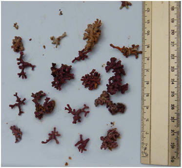
Video Transect 1.
This transect showed a large plain
of uniform ripples with large red algae present at the ripple peaks, at the
peaks there was also a aggregation of bivalve shell and larger sediment.
|
Video
Transect 2.
This
transect initially showed similar results to video 1, however the vessel
moved across the transition between ripples and flat, finer sediment, with
seemingly little biota. |
Video Transect 3.
This was altogether different, with large red algae assemblages, and large
numbers of echinoderms |
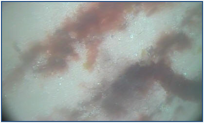
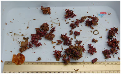
Figure 4.1: Still from
camera tow at site 1. Notice parallel ripples with reg macroalgae.
|
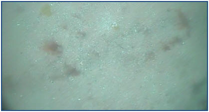
Figure 4.2: Still from
camera tow at site 2. |
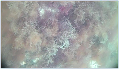
Figure 4.3: Still from
camera tow at site 3. |
| |
|
Grab 1
VIDEO: 50o06.840N, 05o04.800 W
An area of linear ripples with red macroalgae dominating at the
ripple peaks and causing build up of bivalve shells. A few
Asteroidea were visible with some juvenile fish sheltering in
the algae.
GRAB: 50o06.839N, 05o04.784 W
Time: 1103GMT
Depth: 16m
Fauna: Maerl, Tube worms, Bivalves, Amphioxious, Amphipod
The grab showed the sediment to be coarse fragmented shell sand,
with large amounts of dead and alive Maerl. Unidentified
Polychaete tubes were found on a few larger shell and Maerl
fragments. |
Grab 2
VIDEO START: 50o06.932N, 05o04.811 W
VIDEO FINISH: 50o06.947 N, 05o04.722 W
A
flat bedded area of fine sand, indicating a fast moving underlying
current near the benthos.
GRAB: 50o06.934N, 05o04.745 W
Time: 1143GMT
Depth: 16.5m
Fauna: Bivalve – veneroidia, Polycheate – neridie,
Dead maerl
Few
organisms present due to low nutrient availability and unstable
substrate.
|
Grab 3
VIDEO: 50o 08.258 N, 05o 03.335 W
GRAB 3: 50o 08.2604 N, 05o03.3417W
Depth: 17.5m
Time: 1235GMT GMT
Fauna: Ascidacia, Bryozoan mat, Red & Brown varieties of
Fucus, Polychaete tubes
Maerl (living and dead)
|
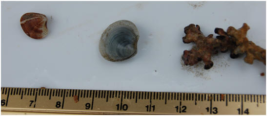
Grab 4
500 08.2604 N 050 03.3417 W
Depth: 17.5m
Time: 12:42 GMT
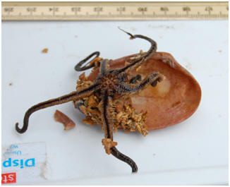
Fauna: Ophiuroidea sp, Nemertean worm, Nereid worms,
Psmmanchus, Gastropod, Bivalve Chlamys, Ulva sp,
Sipunculid
Note: At site 3, the first benthic
grab was a partial mis-fire, so the sample volume was small. In
order to gain a larger sample size, a second grab was taken.
|
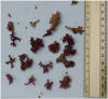 |
Figure 4.4 Lithothamnion sp |
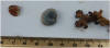 |
Figure 4.5
veneroidia, Polycheate – neridie,
Dead maerl
|
 |
Figure 4.6 Maerl, living and dead |
 |
Figure 4.7 Ophiuroidea sp |
Site 3 marks a benthic boundary
with ripple formations on one side and none on the other. One grab was taken
either side of the benthic boundary. Both grab samples were dominated by
Maerl, with the second grab being over 80% Maerl. The benthic substratum at
this site was hard with many rocks for sessile fauna such as the Sipunculid
to attach to, with fine sandy mud in between the rocks. Most of the fauna
recovered from the samples were either mobile or sessile epifauna, with a
few burrowing fauna also recovered. Grab 3 was dominated by Ophiuroids and
Grab 4 by tube-building polychaetes. The wide variety of fauna recovered at
this site can be interpreted as evidence that even the smallest change in
benthic conditions can completely change the biotope. |
|
Discussion
The data show a variation in
biota with sediment type. The change in biota between sites may be down to
food availability and stability of substrate, both a function of sediment
type and bottom currents. Food availability changes in a variety of ways,
the feeding mechanism of the organism is an important factors, whether it is
a deposit or suspension feeder or detrtivore etc, meaning for example, if
the organism concerned is a suspension feeder, there needs to be certain
levels of suspended biogenic particulate material to feed on, or if the
organism is a detritivore there needs to be certain levels of benthic
detritus available. Food availability is in turn affected by sediment type,
as from differing bacterial breakdown rates from different sediments. So,
sediment type is affected by bottom currents, which in turn affects the
potential organisms present from the feeding methods made available, which
are in turn reliant on the correct sediment type, which is controlled by
bottom currents. There is therefore a very succinct feedback loop between
biota and sediment which can be seen from the change in biotopes between
sites. Grab 1 shows an area limited on potential substrate for algae, which
therefore limits the other organisms able to survive, the lack of large
numbers of echinoderms as with grab 3 shows that either the flow rate is too
great, not allowing settlement of biogenic matter for suspension or deposit
feeding invertebrates, and therefore not providing the diet for echinoderms.
Grab 2 shows a site of little to no biota, with the fine sediment present
being unable to sustain many macrofauna. This fine sediment may be present
due to low flow rates, which may also be affected the present biota. The
lack of substrate available explains the sudden decline in algae. Grab 3 as
mentioned above seems to be the most diverse biotope, with the greatest
abundance of organisms. |
|

The estuarine and offshore environments are characterized
by differing physical conditions. The estuarine environment is dependent on
the mixing of fresh and seawater members, with the biological, physical and
chemical interactions often a function of this frontal mixing system. If the
estuary is large enough then tidal pumping will be affected by coriolis and
also affect conditions by skewing the flow. Estuaries are therefore
halocline controlled, with little affect from temperature. Nutrients are
consistently high and rarely a limiting factor, whereas in the offshore
environment nutrients are often limited in surface waters towards the end of
summer, where waters masses are trapped in surface layers by seasonal
thermoclines. Phytoplankton growth is therefore mainly a function of
nutrient availability, whereas within the estuarine environment, where
attenuation coefficients are an order of magnitude greater, light is often a
limiting factor, with the well mixed tidally pumped waters relatively
consistent with nutrient levels. Both systems are significantly influenced
by the tides, with diurnal changes in the offshore environment from internal
waves and changes in tidal currents, and with the estuarine currents
dominated by tidal flow. The tide is the one factor that ties the two
together and has consequences in both.
In the estuarine environment, the tide dictates
influences the physical structure of the water column. The tidal flow in the
Fal estuary is part of a two layer water column with the high energy tidal
flow moving on top of a low energy body of water. This two layer flow was a
quantified as turbulent at the mouth of the estuary and partially mixed
further towards the source. Furthermore, it was established that the entire
water column was partially mixed/turbulent apart from a bottom boundary
laminar layer that prevented bottom-boundary turbulence, a characteristic of
partially mixed estuaries.
The offshore environment was found to be a continuously stratified
throughout the tidal cycle. Internal waves caused by the river plume of the
estuary were shown to effect key mixing and transport parameters of the
offshore water column. The properties of the internal wave (period,
wavelength, phase velocity and frequency) were shown to change in accordance
with the tidal cycle.
Where these
systems meet, the transition zone has a variety of characteristics, common
in both. This investigation has allowed for data to be taken on the
differences between the systems, and the dynamic character of the estuarine
environment in relation to the more stable offshore conditions.
|
|
References
Callista -
http://www.soes.soton.ac.uk/resources/boats/vessels.html Accessed on 4
July 2010
Fal and Helford Management Forum,
Fal and Helford: Marine Special Area of Conservation Management Scheme,
Fal and Helford SAC Management Scheme, 2006, pp. 8-15
Geyer,
W. 2000. the dynamics of a partially mixed estuary. Journal of Physical
Oceanography. 30. 2035-2048
Grasshoff, k., K. Krenling, M. Ehrhardt (1999). Method of Seawater
analysis. 3rd ed. Wiley – VCH.
Helfrich, K., Melville. 1986. Transcritical two-layered flow over
topography. Journal of fluid mechanics. 178. 31-52.
Klymak,
J. & Moum, J. 2003. Internal solitary waves of elevation advancing on a
shoaling shelf. Geophysical research letters. 30
Langston, W.J., Chesman, B.S., Burt, G.R., Hawkins, S.J., Readman, J. and
Worsfold, P. 2003, Site Characterisation of the South West European
Marine Sites: Fal and Helford cSAC, Marine Biological Association,
Plymouth.
Nash Moum, J. 2005.
Pirrie, D., Power, M.R., Rollinson, G., Hughes, S.H.,
Camm, G.S. and Watkins, D.C. no date, Mapping and visulisation of the
historical mining contamination in the Fal Estuary,
Cornwall, [online], Available: http://projects.exeter.ac.uk/geomincentre/estuary/Main/intro.htm
[accessed 2010, July 6th].
JNCC Fal and Helford SAC Site details, [online],
Available: http://www.jncc.gov.uk/protectedsites/sacselection/sac.asp?EUCode=UK0013112
[Accessed 6 July 2010]
Map images from Google Earth
www.earth.google.co.uk [Accessed
3 July 2010]
Tides and Weather:
www.bbc.co.uk/weather/coast/tides/southwest [Accessed 5 July 2010] |
|


