
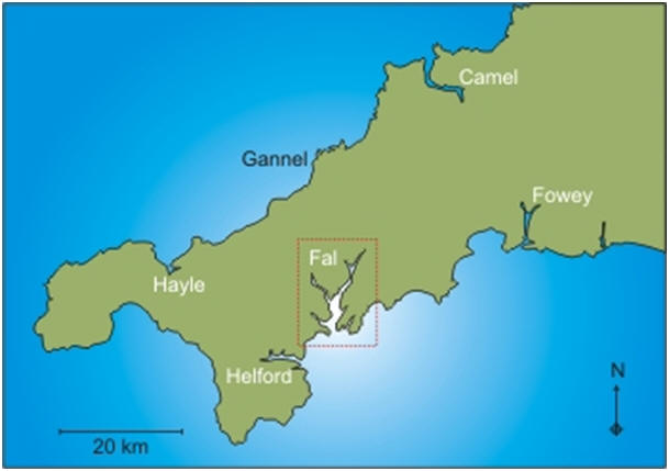
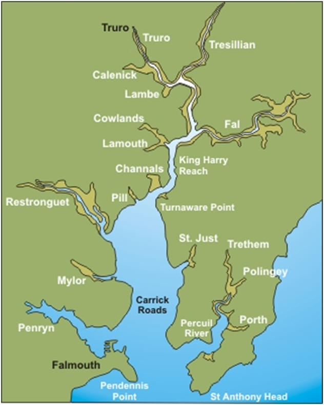
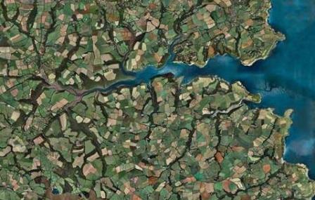
The Fal estuary is located in the southwest of England and gives the town of Falmouth its name. It extends 17Km from the open coast at St Anthony and Pendennis Heads to the Head of the Tresillian River.
The geology of the estuary largely consists of granite and metamorphic rock.
It is classified as a Ria (drowned river valley), and was formed at the end of the last ice age and into the Holocene epoch. During the last ice age, glacial movement cut a channel through the area (giving the estuary its depth). Since the melting of the glaciers (due to climate change), sea level has risen by 15m due to the addition of water into the oceans, resulting in the formation and subsequent flooding of a river valley. The melting of the glaciers after the ice age has resulted in isostatic rebound. The weight of ice over Scotland and Northern Europe put a lot of pressure on the land. Once this pressure was released, the land started to rise, tilting the UK towards the south and giving a larger rise in sea level than other parts of the country.
The channel cut by glaciations resulted in the Fal estuary being the 3rd largest natural harbour in the world, with depths reaching 34m in places. This makes the estuary ideal for shipping channels and moorings. There are two main ports along the estuary at St. Mawes and Truro, making the estuary important commercially, as well as for recreational and fishing purposes.
The Fal estuary is classed as a Special Area of Conservation, SAC, by English Nature, due to its rich diversity of biota (Langston et al. 2003), and support of rare, endangered or vulnerable biotopes and species; listed in the Annexes I and II of the Habitats directive.
Composition of the estuary is predominately sea inlets making up 60%, with tidal rivers; estuaries; mudflats; sand flats and lagoons comprising 35%, the other 5% salt marshes and sand beaches (JNCC, 2010). Some species to note are Maerl (Phymatolithon calcareum and Lithothamnion corallioides), eelgrass (Zostera marina and Zostera noltei), and shore dock (Rumex rupestris) (JNCC, 2010). The total area of the SAC is 6387.8ha.
However various threats are posed to the environment in a number of different forms. Main pollution pressures are from nutrients, sewage, TBT, metals and synthetic organic compounds (endocrine disruptors). As the catchment of the Fal is predominantly rural, arable farming and thus eutrophication into the upper estuary is common, although the most common source of excess nutrients are from sewage works. The table below gives estimated values for different sources of nutrients, based on Parr et. al, 1999.
|
Shoreline length |
126.8km |
|
Channel length |
18.1km |
|
Channel width |
0.01-1.75km |
|
Total estuarine area |
2482 ha |
|
Channel depth (sub-tidal) |
0.2-34m |
|
Sub-tidal |
1736 ha |
|
Inter-tidal flats |
653ha |
|
Salt marsh |
93 ha |
|
Spring tidal range |
5.3m |
|
Neap tidal range |
2.3m |
|
Catchment area |
663.5km² |
|
Source |
Nitrogen % |
Phosphorous % |
|
Agricultural |
25-49 |
3-49 |
|
Sewage treatment works |
3-13 |
26-62 |
|
Atmospheric deposition |
2-6 |
1.5-1.8 |
|
Nitrogen Fixation |
<5 |
- |
|
Background |
13-15 |
10-19 |
Mining for Sn, Pb, Cu, and Fe since the Bronze Age has resulted in the estuary having the highest levels of metal pollution in the UK. Millions of tons of tailings have been deposited in Restronguet Creek, which has a major impact on the Fal and thus the estuary. Although little industry remains, dredging; oil spills; TBT; residual drains from old mines and spoilages still contaminate the water (Langston et al. 2003). For example, in 2009, 13,600 litres of waste oil were leaked into Falmouth Docks, and the Wheal Jane incident in 1992, where 50 million litres of acidic (pH 3.1) metal laden water flowed out via Restronguet Creek into Carrick Roads.
A combination of metal and nutrient inputs sometimes causes toxic algal blooms, such as from Alexandrium minutum, or the 1995-1996 bloom of the dinoflagellate Alexandrium tamarense.
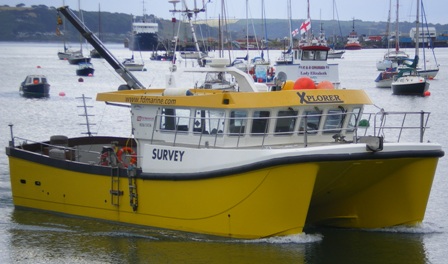
RV Xplorer:
The RV Xplorer is a twin hulled inshore research vessel which can be used to sample in the estuary and offshore. It is operated by the FD marine Survey and is also used for the geophysics practical.
Specification
Length:12.0m
Draft: 1.00m
Beam: 5.2m
Speed: 25 knots (max)
Passengers: 12 passengers plus crew
Capstan: Anchor retrieval
Range from safe haven: 60 mls
Large working deck with winch, 1.5 ton capacity
Beam: 5.2m
Equipment
Hydraulic crane with winch, 1.5ton.
Lacking in processing labs
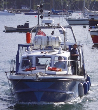
RV Bill Conway:
The Bill Conway is a small scientific vessel used to take samples and survey in the estuary. The vessel is a Lochin 38, it operates out of Southampton and at sea up to 60 miles from a safe haven. The boat has a large open deck and a spacious wheelhouse, equipped with lab benching and a sink.
Specification
Length: 11.74m
Beam: 3.96m
Draft: 1.3m
max Speed: 10knots
Passengers: 14 including crew
A-Frame in stern: 750kg 3m max height
Davits: 1x50kg
Trawl Winch: max wire length 70m
Range from safe haven: 60mls
Freeboard to Working Deck: 1.0m
Cruising Speed: 9 knots, range 150 nm
Maximum Endurance: 1 day at sea
Equipment
Two davits, 50kg capacity
A frame with 750kg capacity
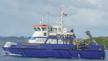
RV Callista:
The RV Callista is a twin hulled offshore vessel with three deployment points. The vessel can be used for sampling both in the estuary and offshore.
Specification
Length: 19.75m
Cruising speed: 15kts
Beam: 7.4m
Passengers: 30+4 crew
Draught: 1.8m
A-Frame: 4 tonne capacity
Capstan: 1.5tonne pull
Davits: 2x100kg
Range from safe haven: 60mls
Depth midship: 2.85m
Equipment
Two side davits with hand winch, 100kg capacity
A frame with 4 tonne winch at the rear
Wet and dry labs
Vessel has kitchen, toilet, sleeping facilities
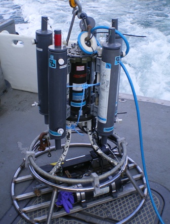
Scientific equipment:
Fluorimeter
Transmissometer
CTD and rosette
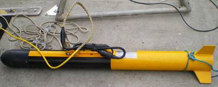
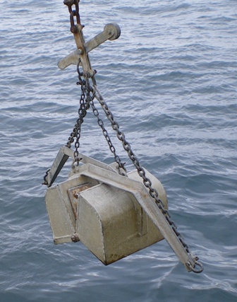
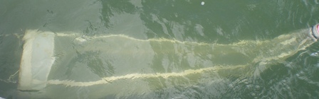
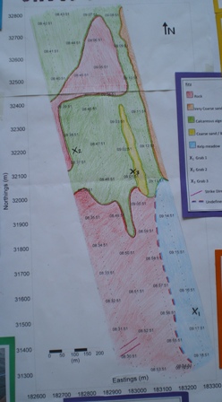
•To identify specific biotopes and benthic sediments in the estuary by surveying specific transects using a sidescan, then focusing on a particular area of interest identified from the sidescan tracer using the Van Veen grab.
•Use the side scan sonar to give an overview of the seafloor and bed formations.
•To produce a geophysical and biological benthic map of transects.
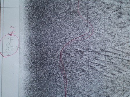
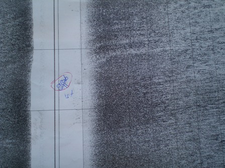
The tracing was cut in to segments representing each transect and aligned for analysis. Different areas showing different habitat features were identified by differences in shading and texture, boundaries were then located. A track plot was created on Surfer showing the track of the boat by time and at different locations (Eastings and Northings). The different areas of the habitat were then transferred to the benthic map from the tracing. The shading of the tracing was dependent on the intensity of the backscatter of the sound wave of the side scan sonar. Fragments needed to be greater than 3mm to appear on the tracing, this was calculated from the equation :
V=Fλ
1500m/s=450KHz x 3mm
Rock appeared white with dark shadows due to strong reflections, however calcareous algae and broken shells appeared darker due to many fragments causing intensified scatter. Coarse sands appeared paler as more energy was absorbed than reflected. Areas were seen to have extensive kelp meadows from using video and grabs samples but these did not appear on the tracing as kelp and seaweeds have the similar densities to water so appear transparent to the side scan sonar.
To transfer the benthic areas to the side scan map the tracing had to be scaled. To do so the width of the tracing must be measured and then compared to the known 150m swath width
Fig.4.14: Sidescan interpretation method.
Fish Height (Hf ) was calculated by measuring the distance from the fish track to the seabed on the tracing ( 2.5cm), which was converted to actual distance (12.25m). R is the slant swath and is the measurement from the fish track to the change in boundary. To calculate the true range (Rh) Pythagoras theorem was used. E.g. Rh2 + Hf2 = Rs2. Rs is the Slant range. The process was repeated for each change in benthic habitat in order to plot the areas onto the scaled side scan plot by using ratios of measurements. Grab sites were also plotted on to the map and the areas coloured and a key created.
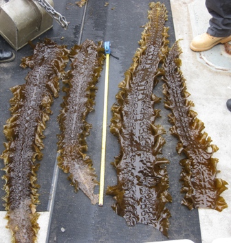
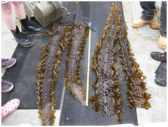
Such as the sea belt Laminaria saccharina. This is a green brown sea weed usually found attached to rock. The sample we collected had Bryozoa attached to its surface.
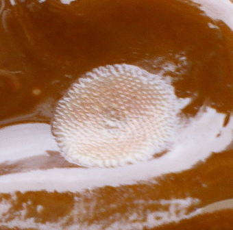
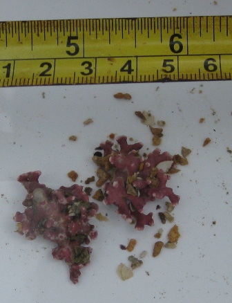
Maerl was found on granite collected from the grab.
A type of sea snail, believed to be Gibbola cinerari was identified. It had 4-5 whirls on its grey/brown/brick red shell. This was found on the kelp.
Repeat 1: Kelp was collected in the second grab (repeat of grab 1). It was smooth, green/brown, with no spots.
The sea bed was identified to be a kelp forest growing on rocky substrata, so little sediment was collected.
Repeat 2: A small brittle star (Ophioroid) was collected but its species was not identified on the boat.
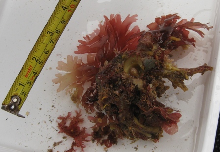
Red seaweed was identified and was thought to be Nitophyllum punctatum. It was smooth, thin, red/pink.
An hermit crab was collected. The species was not identified.
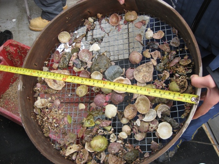
Sieving the sample revealed large numbers of Maerl. This sample appeared to have more diversity than grab 3.
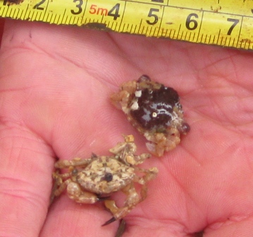
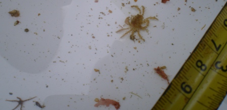
A number of organisms were found; including several unidentified crab species
1. Hermit crabs
Crab with black carapace (1cm wide) and white legs. Large posterior appendages.
3. Sandy coloured carapace (1.4cm wide)
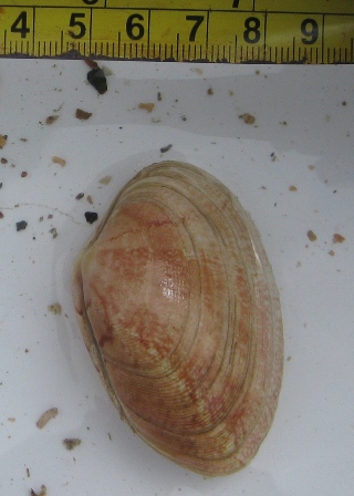
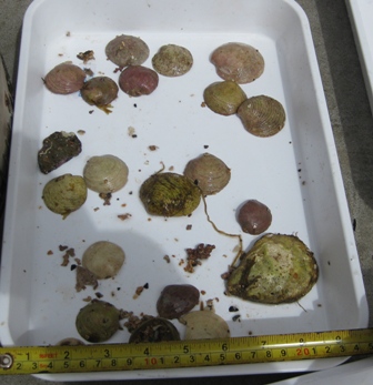
Several Bivalve shells were collected, most of which were dead. E.g. Astarte sulcata.
The live bivalves found were difficult to identify as the inside of the shell could not be examined (for example teeth).
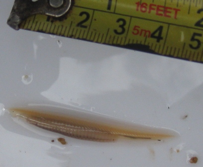
One of the unidentified living bivalves was this 2 inches wide, with
cream and brown/orange shell:
Small amphipods were also collected at this grab station but they were unidentified.
Falmouth Group 5 Video 1: http://www.youtube.com/watch?v=RXReIX8YV-M (Kelp meadow)
Falmouth Group 5 Video 2: http://www.youtube.com/watch?v=ajvzRw8af9s (coarse sediment area)
![]()

![]()
![]()
A geophysical survey was conducted in Falmouth Estuary in order to determine the marine benthic habitat. The area observed had been studied the previous 4 years, so the survey was for monitoring purposes, and the data that were collected could be used to identify any changes in the biology. This could be due to natural changes such as the tides and seasons, but also due to the invasion of alien species and pollution, as there is a sewage outfall that goes into the estuary. Natural England will view the survey data with the aim of identifying the biotopes in the area. Many rare and important species (such as the calcareous algae Maerl) live in the estuary and it is important that their existence is known so efforts can be made to protect them.
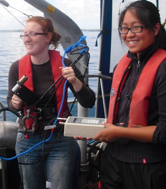
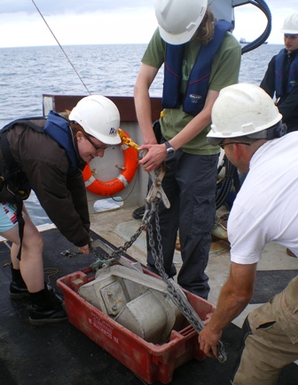
The safety elements of the investigation involved wearing hard hats when deploying instruments and wearing gloves when handling the grab samples.
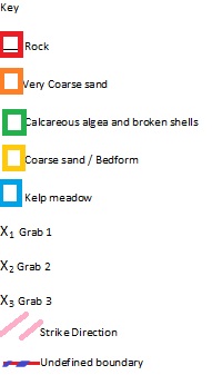
Date: 30/06/2010
Location: Falmouth Estuary
Time: 0800-1300GMT
Weather: Overcast, light breeze
14mph, gusts of 27mph.
Temperature 20⁰C, 8/8 cloud cover.
Excellent visibility.
Tides: GMT
|
Low Water |
High Water |
Low Water |
High Water |
|
00:37 |
06:10 |
12:54 |
18:20 |
|
1.1m |
4.9m |
1.1m |
5.1m |
Biotopes:
A biotope is an area of homogeneous environmental conditions where a specific biological community exists. The idea of biotopes is that they can be classified and applied in other areas of similar surroundings. This can be helpful to understand the degree of pollution in an area and to describe community change.
The Wheal Jane tin mine:
Care had to be taken when handling the samples, as due to a mining accident in 1992 sediment could still contain traces of copper, tin, arsenic and other heavy metals. The Wheal Jane tin mine flooded causing roughly 50 million litres of water with a high heavy metalloading and very low pH of around 3.1 to be released into the river Fal. An extensive cleaning operation was carried out however traces could still remain.
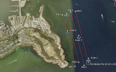
Four transects parallel to the beach were sampled, the transects were taken 100meters apart from each other with a 75m swath on each side of the boat, so the total swath was 150m. The transects then overlapped by 25m to create an accurate overview of the sea bed substrate. Measurements were taken at high frequency (415 KHz). The latitude and longitude were recorded every minute to record the exact position of the boat during the transects.
The side scan was deployed at point 50°08.8351’N 5°02.3934’W creating a side scan tracer along the four transects. The GPS location for the side scan needed to be corrected as the GPS on the Xplorer is located on the back of the boat and the tow fish was attached to the back of the boat by a rope (542cm long) creating a horizontal difference between the distance recorded and the actual.
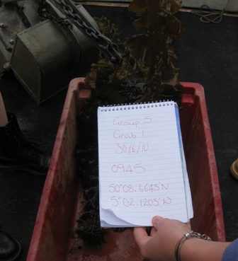
The side scan tracer was checked and 3 sites were chosen to conduct grab samples. At the first site three repeats of the grab sample were conducted due to the rocky substrate, which made it difficult for the grab to pick up the sediment. At this site mainly seaweed (Kelp) was found. Only one sample needed to be taken at the other two sites.
At sites 1 and 2 the video camera was deployed after the grabs were taken in order to view the seabed clearly as the boat drifted with the current, this provided a more complete understanding of the sea bed topography and substrate at these sites.
To process the side scan data the four segments were placed to correspond with their positions in the estuary. The lengths of the scans was different due to the boat moving at different speeds at each transect. The speed was altered by the tides, for example the landward ebbing tide made the track towards the land longer. To produce the benthic map various equations were used to ensure the distances plotted on the map were accurate on the sea bed, as the depths recorded were the slanted depth “slant swath range (r)”.
Transect Locations:
Table.3.2: Transects
|
Transect Number |
Position |
Time (AST) |
||
|
Start |
Finish |
Start |
Finish |
|
|
1 |
50˚08.6180 05˚02.3827 |
50˚09.2300 05˚02.5984 |
0832 |
0842 |
|
2 |
50˚09.2440 05˚02.5173 |
50˚08.6648 05˚02.2953 |
0844 |
0852 |
|
3 |
50˚08.6300 05˚02.1985 |
50˚09.2650 05˚02.4451 |
0857 |
0907 |
|
4 |
50˚09.2727 05˚02.3560 |
50˚08.6622 05˚02.1220 |
0909 |
0917 |
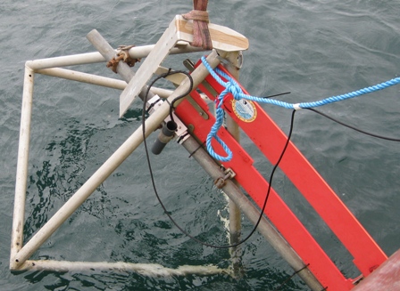
Grabs:
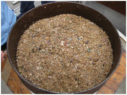
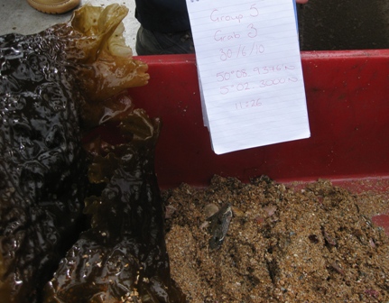
From the side scan sonar trace, 3 sites were chosen at which to take a grab sample, using tonal changes to identify different substratum. The first grab site chosen was unsuitable; after 2 repeats it was decided that the rocky strata was not giving us informative conclusive results. For the following 2 grabs therefore, a video camera was used in order to get a better overview of the site.
Table.3.3: Grab positions and times
|
Grab Number |
Position |
Time (AST) |
|
1
|
50˚08.6643 05˚02.1200 |
0940 |
|
1 (2) |
1000 |
|
|
1(3) |
1005 |
|
|
2 |
50˚08.9963 05˚02.5115 |
1055 |
|
3 |
50˚08.9380 05˚02.3032 |
1126 |
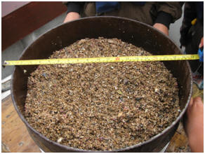
The sediment size in grab 2 was largely granule size (phi-unit: -1, ~2mm). There was also the occasional cobble sized fragment (of granite, metamorphic rock and shell fragments). More live Maerl was found in this grab compared to grab 3.
The sediment size in grab 3 was also mostly granule size (phi-unit: -1, ~2mm). Again, there was also pebble and cobble sized fragments. The grab was similar to grab 2.
Analysis of the data from the side scan revealed the majority of the area was composed of rocky reefs covered by kelp meadows. With another area of calcareous algae and broken shells. Grabs were taken in the following substrata: grab 1 in a kelp meadow area; grab 2 in calcareous algae and broken shells area; and grab 3 in coarse sand with calcareous alage and shell fragments. The grab from the kelp meadow did not give a sediment sample, as it overlay a rocky bed. Sieve analysis of grabs 2 and 3 revealed the density of Maerl was higher in grab 2, which corresponded to a greater species diversity, such as bivalves, amphipods, crabs etc.
Overall, the sample area surveyed can be classified into two main biotopes. The first of these is the kelp forests and meadows which are likely to provide food and shelter for many marine species. The rocks themselves provide a substratum for the kelp, and many organisms are likely to live within the cracks and crevices. The second biotope consists largely of Maerl growing on course sediments and shell fragments. The presence of Maerl is significant as it is a protected species.
The area of the estuary that was surveyed is a special area of conservation (citation) and if the construction of the proposed shipping channel was approved and dredging was to take place at this part of the estuary, there will be drastic consequences for this ecosystem.
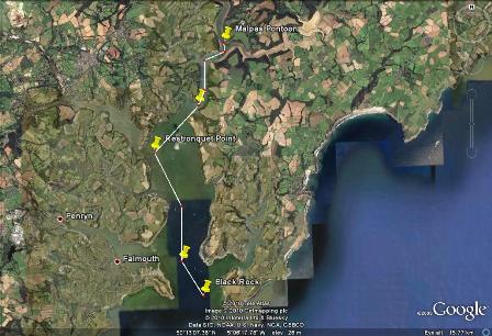
In order to gain a good understanding of the Fal estuary a plan was drawn up to locate potential areas of interest on the estuary. Areas of interested included the mouth of the estuary, three locations in the mid estuary with specific characteristics such as, an adjoining dock, contaminated creek and a significant change in width of the estuary. A final station was selected near Malpas, the furthest possible landward location within the time constraints. All transects had a station located in the centre of the transect.
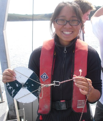
Transects were drawn (see results for lat and long) across the mouth of the estuary and the three other stations. Here ADCP transects were taken to gain an understanding of current speed and direction throughout the water column. At station 5 near Malpas an ADCP transect was not possible. At all stations a CTD profile was taken, this enabled salinity, temperature and transmission to be plotted against depth at all five stations. Five Niskin bottles were attached to the CTD Rosette and were fired at depths where there were noticeably different water masses on the CTD monitor, this was so samples of differing characteristic could be analysed for changing nutrients, oxygen and biology. Further sampling was carried out insitu, where water pump samples were collected every half salinity unit change for surface mixing analysis. The plankton net was deployed at stations 1, 2 and 5 for organism analysis. Lastly the secchi disk and light attenuation probe were deployed at all stations, this gave evidence for suspended particulate matter and light penetration depths relating to phytoplankton growth.
(All transects were conducted from East to West)
Transects were drawn (see results for lat and long) across the mouth of the estuary and the three other stations. Here ADCP transects were taken to gain an understanding of current speed and direction throughout the water column. At station 5 near Malpas an ADCP transect was not possible due to the shallow water surrounding the thin deep water channel.
Transect 1
Velocity magnitude shows there is not much flow at this transect, due to the tide being at a turnaround point between flooding and ebbing. Average flow would be approximately 15-20cm/s. It is clear that there is faster flow reaching 0.300m/s on the flats east and west of the deep water channel, whilst flow in the channel itself is much slower at approximately 0.100m/s. Higher flows indicate disturbance and eddying from the shallower depths, particularly on the eastern shelf. Velocity direction is very sporadic, evidence of high rates of shear and turbulence as the tide switches. The 3 higher backscatters averaging 90dB at 58m, 616m, and 1278m show interference; motor boats passed at these points.
Transect 2
A similar effect as transect 1 is seen, whereby
velocity is at a faster rate reaching 0.400m/s on the flats than in the
deep channel, where it is a fairly uniform 0.080m/s. Flow at shallower
depths up to 10m is generally southerly, i.e. ebbing out of the estuary,
which corresponds to the state of the tide. Considerable turbulence in
the deep channel is evident, with flows in all directions. Composition
of the bed can be estimated using the backscatter – on the west, where
backscatter is high, up to 90dB, mud is likely to be the dominant
sediment, whilst on the east where backscatter has lower values of
60-70dB, rocky strata is likely to dominate. The higher backscatter
within the water column is likely to be from plankton reflection.
It should be noted that the full extent of the channel is not shown, as
the ADCP had not been set up correctly.
Transect 3
In comparison to transects 1 and 2, the velocity magnitude appears more uniform across the whole transect, in both the flats and the deep channel averaging 0.052m/s. A higher velocity reaching 0.5m/s on the western flat could be the result of a back eddy or feature on the seafloor. Velocity direction is again generally southerly, due to the tide ebbing. Backscatter again shows high values of 90dB on the western flats, indicating a muddy sediment.
Transect 4
Velocity magnitude varies laterally in this profile with higher flows up to 0.488m/s at the surface, gradually decreasing within the main channel to 0.094m/s at the bottom. Tidal direction is on the whole in a southerly direction, although in the main channel some significant eddies are evident as the flow varies, even completely reversing at 311m along the transect. Backscatter in the water column averages 74dB, a value higher than observed at other stations and thus could indicate a higher productivity water column.
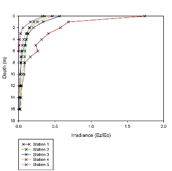
Light data:
The irradiance showed a general trend of increasing down the estuary. Station 1 had the highest irradiance of a ratio of 1.74. The ratio decreased with depth for every station as the attenuation of light decreased through the water column.
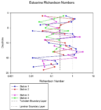
Richardson's number:
The Richardson numbers were calculated at each site at 1m intervals, due to the very mixed nature of the estuary and no obvious stratification or front from the ADCP. A Richardson number below 0.25 indicates turbulent flow, between 0.25 and 1 indicates partially mixed water, and above 1 laminar flow predominates. As can be seen from the diagram, at all sites the principal flow was turbulent, i.e. a Ri of below 0.25. This is due to tidal mixing, turbulence and shear in the water column, and furthermore the constant flood and ebb of the tide preventing stratification occurring. At stations 2 and 4, the flow was never laminar, although at 1 and 3 there were certain depths where laminar flow occurred. Increased turbulent flow at stations 1, 2 and 3 is the result of bottom stress and shear. Overall, the Richardson Numbers imply the estuary is well mixed, with high levels of turbulence causing fresh and saline water to combine.
|
Track |
Start |
Finish |
||
|
Position |
Time GMT |
Position |
Time GMT |
|
|
1 |
50°08.376N 05°01.013W |
0831 |
50°08.591N 05°01.481W |
0845 |
|
2 |
50°09.293N 05°01.481W |
1006 |
50°09.353N 05°01.941W |
1016 |
|
3 |
50°11.480N 05.01.773W |
1139 |
50°11.190N 05°01.136W |
1153 |
|
4 |
50°12.160N 05.02.125W |
1254 |
50°12.274N 05°02.399W |
1258 |
| Station | Secchi Depth (m) | k | Euphotic depth (m) |
| 1 | 7 | 0.2 | 21 |
| 2 | 5.4 | 0.3 | 16.2 |
| 3 | 3.5 | 0.4 | 10.5 |
| 4 | 3 | 0.5 | 9 |
| 5 | 1.4 | 1.0 | 4.2 |
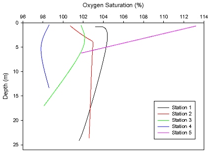
Oxygen profile:
Looking at the graph it is noticeable that stations 1 to 3 towards the mouth of the estuary have a similar trend throughout the water column. Oxygen saturation at all three stations increased within the first 5 metres and then decreased and in one case at station 2 stayed constant for the rest water column. Station 4 began at 99% saturation at the surface and then decreased to 98% at 5 metres only to increase after this point. Lastly station 5 began at an extremely high saturation of nearly 114% a the surface and decreased rapidly to 102% in only 6 metres of water.
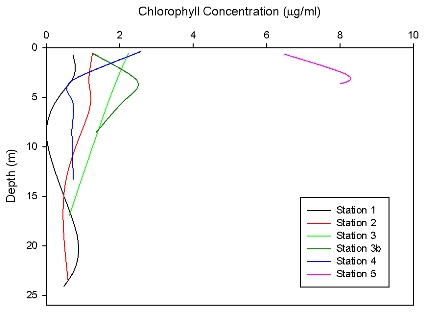
Chlorophyll profile:
At the surface the chlorophyll values increased from station 1 to station 5. There was a gap of about 4µg/l of chlorophyll between station 4 and 5. Chlorophyll decreased with depth at all stations, the chlorophyll peaked at different depths and followed different trends at each station.
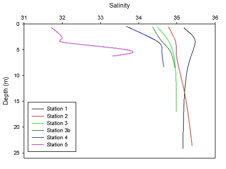
Salinity Profile:
The salinity profiles show a general increase in salinity with depth at all stations excluding station 1. Station 5 shows the greatest variation and at the shallowest depths. The overall trend is that of decreasing salinity through the stations as the measurements were taken further up the estuary.
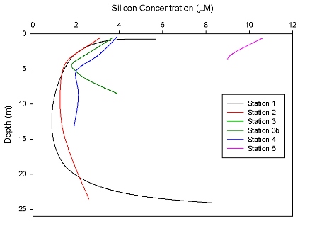
Silicon Profile:
The general trend of silicon was to peak at the surface and at depth, with lowest values around the middle of the water column. Stations 1 to 4 where generally much lower than station 5 and station 1 shows greatest variation with depth.
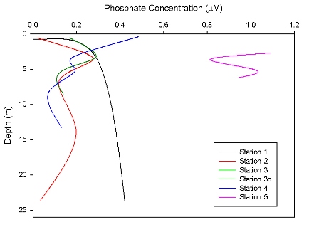
Phosphate profile:
Stations 1 to 3 showed peaks in phosphate at around 4m depth, and a second increase around 15m, station 4 showed highest concentrations at the surface and Station 5 showed greater concentrations than the other four stations
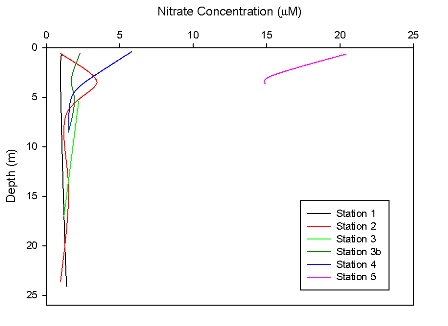
Nitrate profile:
Stations 1 to 4 show similar low Nitrate concentrations of between 0 – 5µM, with the general trend of decreasing with depth. Station 5, highest up the estuary, shows an increased Nitrate concentration surface value of 20.4µM decreasing with depth to 8.6µM.
Mixing Diagrams:
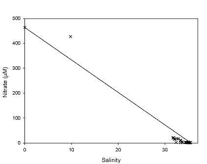
Nitrate Mixing Diagram:
Nitrate samples show deviations from the theoretical dilution line thus demonstrating non-conservative behavior. Higher salinities have lower concentrations than expected, possibly representing removal of nitrate and lower salinities could possibly show addition but with too few samples it is inconclusive.
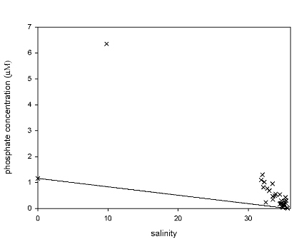
Phosphate Mixing Diagram:
Phosphate samples where found to be generally higher than the theoretical dilution line, showing non-conservative behavior, with addition occurring throughout most the estuary.
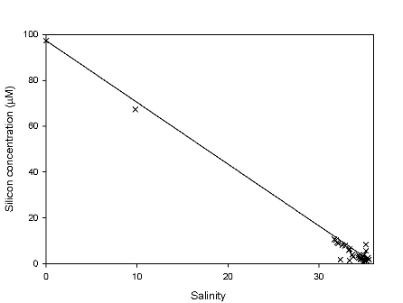
Silicon Mixing Diagram:
Silicon values follow the theoretical dilution line, showing conservative behavior, as such little silicon is added or removed along the estuary.
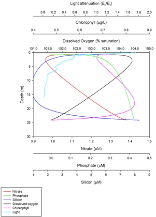
Station 1 info:
At station 1 light attenuation decreases with depth from 1.7 at the surface to 0.0 below 12m depth. Chlorophyll generally decreases with depth, with a peak at 0.85µg/L at 20m depth, which may be due to migration, due to the lack of light attenuation at this depth. Dissolved oxygen decreases with depth, with a peak at 4m depth at 104.4% and decreasing to 101.5% at 24m, suggesting photosynthesis activity in the surface layers, which is not supported by the chlorophyll data. Nitrate concentrations are lowest (0.95µM) at the same depth as the percentage oxygen saturation is at its highest, and increases with depth to 1.39µM, suggesting activity of phytoplankton. Phosphate levels are also found to increase with depth from 0.0µM at the surface to 0.42µM at depth. Silicon concentrations appear to be high at the surface (5.8µM), then decrease with depth to 1.3µM and peak again at the seabed to the highest value of 8.5µM. This may be due to sampling or measuring errors, or it may be due to presence of silicon at the surface and remineralisation of diatoms at depth.
Tres = Total residence time
Smean = 34.11
Ssea = 35.49
Vtotal =12634177m3
R = rate of estuarine discharge = 0.648
((1-34.11/35.49) x Vtotal)/0.648
=758132.36s
=8.77 days
To calculate the residence time of the estuary the river flow rate into the estuary is needed. The figure of 0.648 was used as this was the lowest on the records, as the riverine input is currently the least it has been for 80 years. The residence time of 8.77 days is a relatively long time, and this makes it difficult to use the mixing diagrams to estimate the mixing of the estuary with confidence. This is also due to the fact that because of the low rainfall and riverine input, the salinity gradient throughout the estuary does not differ by much, going from 30 to 35.
The Silicon mixing diagram (fig.5.16) indicates conservative behaviour, with simple mixing between the riverine and ocean end member and with no addition or removal throughout the estuary. Silicon levels are relatively low throughout the estuary, this may be due to the fact the samples were undertaken after the plankton bloom, indicated by low plankton levels, when silicon has been utilised by diatoms and sunk through the water column and possible been grazed by the zooplankton. (Loder & Reichard. 1981). However the Nitrate and Phosphate samples (fig.5.14 & fig.5.15) indicate non conservative behaviour and therefore lack of simple mixing within the water column. There is a possibility of addition towards the riverine end member, also supported by increased nutrient levels in station 5 (at the top of the estuary) and decreasing down the estuary (fig.5.13). This addition may be a result of agricultural runoff (Miller.2004) introducing increased nutrients into the Fal estuary, this may be due increased rainfall the previous day to the sampling. Addition may also be due to remineralisation of nutrients after the spring phytoplankton bloom, by grazing and excretion by zooplankton. (Miller.2004) This is supported by the increased zooplankton obtained from the site highest up the estuary. (fig.5.19) Increased nutrients supports a larger population of phytoplankton, indicated by the higher chlorophyll levels also found in station 5. (fig.5.9) (Miller. 2004). Nitrate is also potentially removed in higher salinities, closer to the seaward end member (fig.5.13) This may be due to uptake by phytoplankton, for use in DNA, proteins and enzyme co factors (Miller. 2004).
Estuarine mixing diagrams are based on the assumption that the system is in a steady state (Loder & Reichard. 1981), however as the flushing time of the Fal estuary is 8.77 days which is greater than a few days, the changes in end member concentrations will affect the shape of the mixing curve, resulting in an inaccurate interpretation. Also the end members for the phosphate data (fig.5.15) may be inaccurate, changing the conservative behaviour, this may be due to collecting them at a different time to our samples.
Oxygen concentration (fig.5.8)has been found to decrease with depth, which indicates phytoplankton are photosynthesising in the surface layer and there is increased zooplankton respiring at depth. This increase in oxygen at the surface is supported by the increased light attenuation in the surface of the water column (fig.5.6) as photosynthesis by phytoplankton decreases with depth (Miller. 2004). Most stations appear mixed with fairly homogeneous oxygen saturation throughout depth, which is supported by the absence of distinct thermoclines and haloclines at the majority of stations (fig.5.17).
Salintiy (fig.5.10) is shown to increase with depth and increase down the estuary. Station 1 has a more uniform water column with little difference in salinity and temperature with depth, indicating increased mixing supported by Richardson’s numbers of below 0.25. Station 2 and 3 are situated by river mouths meaning a more distinct thermocline and halocline are formed as lower density, warmer freshwater flows on top of the denser, more saline, cold sea water. This is evident from the CTD data as well.
The results are inconclusive as certain variables do not correlate and a conclusion cannot be accurately drawn from our data sets. This may be due to short term fluctuations of riverine concentrations due to changes in turbidity (Morris et al. 1981). As the samples were only collected over a short time period, they cannot be generalised to longer time periods, further data must be collected.
Physical structure of the estuary : From the ADCP data and Richardson’s number calculations it appears that the estuary has a well mixed physical structure.
Plankton: The growth of plankton in estuaries is light limited. Turbidity in the estuary therefore effects phytoplankton growth. Little phytoplankton was found on this study, but many zooplankton were collected. This could indicate that the phytoplankton bloom occurred earlier in the season, and that currently the zooplankton are in bloom due to the recent high consumption of phytoplankton.

Aim:
· To determine the mixing and fronts around Lizard point west of Falmouth harbour.

· To study the development of eddies travelling towards Helford estuary.
· And how these physical factors influenced the biology surround Lizard Point.
Location: Lizard Point and Helford Estuary
Time: 09:00-17:00 (GMT)
Weather: Mostly overcast, 7 oktas. Occasional sun and rain.
Tides: High tide: 12:51, Low Tide: 19:34 (GMT)
Introduction:
At Lizard Point there is a steep topography decreasing sharply from 70m to 30m, this induces mixing due to frictional forces from wind and seabed shear. During the summer months the offshore water column is stratified with an obvious thermocline of warm water overlying cold water. These two separate water masses are entrained once the frictional forces act upon them. As the spring phytoplankton bloom is thought to have passed the upper thermocline is likely to be depleted in nutrients while the underlying water is nutrient rich.
Once water begins to be entrained at Lizard Point the cold nutrient rich water mixes with the warm nutrient depleted water, potentially providing good plankton growth conditions. Offshore there may also be continued plankton growth however it is a balance between nutrient and light availability. Offshore water is generally low in suspended particulate matter and therefore does not attenuate light like coastal or estuarine water. As the upper water column is nutrient depleted it is unsuitable for plankton growth, but at the bottom of the thermocline there is some diffusion of nutrients across the two water bodies enabling some plankton growth. As light is likely to penetrate down to the thermocline plankton can grow in the boundary where nutrients diffuse across. This suggests the limiting growth factor is nutrients in offshore water.
Methods
Physical Properties
ADCP transect
Near Lizard point headland, around the sill, there was a high velocity magnitude, averaging 0.440m/s across the entire water column. Moving away from the headland, the magnitude decreased rapidly to between 0.100m/s and 0.250m/s, until the end of the transect at 5000m offshore. A marked magnitude change at 1700m suggests the position of a front. Considerable eddying can be seen throughout the entire length of the transect, but appears stronger within 1271m of the headland, this is due to increased shear and bottom stress due to shallowing waters.
Across the transect, velocity direction varies 90° between North East and South East. Closer to the headland the direction is predominantly South East, indicating refraction from the South Westerly wind and tide direction. Further offshore, the velocity direction is closer to the wind direction as there is less interference from bedforms and the headland, reducing refraction.
A large zooplankton bloom can be detected by a backscatter value of approximately 78dB at 1692m off the headland. The position of the zooplankton matches the position of the predicted front and diminishes with distance from this position. Backscatter from the sea bed of 60dB indicates a possible rocky substrata.
Richardson Number:
The Richardson number was calculated at 1m depth intervals from the start of the ADCP transect, at Lizard’s Point. As can be seen, the majority of values lie >0.25, i.e. of a turbulent nature. At depths 3, 4, 11 and 14m, the Richardson number increases beyond 0.25, i.e. it moves from being turbulent to being partially mixed. If it increased beyond 1 it would be classed as laminar. This data corresponds to the ADCP data, which showed a high velocity magnitude, averaging 0.440m/s combined with refraction from the headland, producing turbulent flow.
Due to the strong thermocline observed at the end of the ADCP transect as can be seen in the CTD data, Richardson number was calculated across this. Above the thermocline, a value of 0.31 was achieved whilst below 0.07 was observed. Considerable stratification is thus evident, with laminar flow in the surface 6m where there are warmer temperatures (averaging 16.8°C), and below the thermocline (averaging 12.2°C), turbulent flow due to bottom stress and shear.
|
Start 1105 |
Finish 1142 |
||
|
49°56.500N |
005°12.243W |
49°53.038N |
005°11.900W |
| Station | Secchi Depth (m) | k (m-1) | Euphotic depth (m) |
| 1 | 7.5 | 0.19 | 22.5 |
| 3 | 9 | 0.16 | 27 |
| 4 | 7 | 0.21 | 21 |
| 5 | 8 | 0.18 | 24 |
| 6 | 9 | 0.16 | 27 |

Fig.6.3: ADCP transect taken on Callista
| Station | Position |
| 1 | 50°07.857N 05°01.898W |
| 2 | 49°56.567N 05°12.202W |
| 3 | 49°56.500N 05°11.791W |
| 4 | 50°05.81N 05°06.41W |
| 5 | 50°05.874N 05°05.313W |
| 6 | 50°05.911N 05°04.121W |
To determine physical processes operating around Lizard Point and how they affected the biology in the area it was necessary to carry out ADCP transects, CTD profiles and plankton and light studies. Firstly a CTD profile was taken at Black Rock, located at the mouth of the River Fal. The profile was taken to act as a control for the offshore data, so estuarine water could be compared to ocean water. The secchi disk and the plankton net were also deployed to 10m at this point.
RV Callista then motored from Black Rock to Lizard Point, roughly 15Nm. Here a CTD profile was taken to study the extent of mixing at the location. A stationary ADCP was also taken to determine current speed and direction throughout the water column at the headland. Then an ADCP transect was taken in a southerly direction for approximately 8Nm. This was carried out to provide information on where the front was located (mixed water becomes stratified) and to show any zooplankton showing up as backscatter in the water column. At station 3 a third CTD profile was taken at the end of the transect to determine the extent of water column stratification and the formation of the thermocline. This could then be compare to the previous profile. The secchi disk was deployed to 9m and the plankton net was deployed twice, once to 17m to sample the full water column below the thermocline and once to 10m to sample water above the thermocline.
It was then decided that the sea state was too rough so sampling took place in Helford estuary (sites 4, 5 and 6). Station 4 was the furthest up the estuary but still in the mouth with the other two stations occurring within the next mile towards the sea. At each station a CTD, a static ADCP, plankton net and secchi disk was taken, with an ADCP transect being taken across all three stations. Refer to map for Site locations.

Table.6.3: Light information at stations
Lab techniques
Data was calibrated to the appropriate instrument before any data analysis took place.
Silicon analysis: Standards were used to produce a calibration line from which the silicon concentration of the samples could be calculated from absorbance values (when mixed with the reagents). (Parsons et al. 1984).
Phosphate analysis: Standards were used to produce a calibration line from which phosphate concentrations of the samples could be calculated from absorbance values. (Parsons et al. 1984).
Chlorophyll analysis: The fluorescence of acetone extracts from filtered samples where measured using a fluorometer to determine chlorophyll concentration. (Parsons et al. 1984).
Winkler’s Titration Method: Used to determine dissolved oxygen concentration (Grasshoff. 1999)
Flow Injection Analysis: Used to determine nitrate concentration (Johnson. 1983)
The graph shows the vertical profile at station 1 taken from the surface to the seabed. All the variables fluctuated through the water column which showed mixing of the water. Temperature decreased with depth from 15 to 12.8°C, a thermocline could be seen between 4m and 8m, where most mixing took place so the salinity changed in a short distance. Salinity increases with depth, first it decreased to 34.8 and then increases to 35 at 7m. The fluorometer readings are high at the top and the bottom decreasing in the middle of the water body. Turbidity tends to decrease with depth peaking at 2m.
The data indicates that the nutrients and chlorophyll values increase with depth but the percentage oxygen saturation decreases with depth.
Station 2:
Temperature decreases gradually from 13.3°C to 12°C. Salinity increases with depth from 0.5m to 26m, the salinity fluctuates throughout the water column generally at 35.06 except for at the surface, 12m and 16m where it decreases. Turbidity remains low after the surface measurements but shows some peaks at 10m and 17m, the fluorometer shows the same trend fluctuation more but staying around 1.05/1.10.
Station 3:
At station 3, temperature measurements showed a clear thermocline between 4.5m and 18.6m, decreasing from 16.8°C at the surface to 10.8°C at depth. Salinity values vary with depth but showed a general increase from 34.9 at the surface to 35.1 at 69m depth. Apart from within the first 3m, where there is a turbidity peak, turbidity remains fairly constant throughout depth. Fluorometer readings show a clear chlorophyll peak between 10m and 26m, which corresponds with the position of the thermocline, indicating the position of the phytoplankton populations.
Phosphate levels increased with depth from 0.0µM at the surface to 0.15µM at 30.8m depth. Silicon levels also increased with depth from 1.0µM at the surface to 2.8µM at 30.80m depth. Nitrate concentrations decreased with depth, with the minimum at 11.8m of 0.7µM. Dissolved oxygen concentration had a peak at 11.8m of 104.7%, corresponding with the Nitrate minimum, suggesting photosynthesis, oxygen concentration then decreased with depth. Chlorophyll concentrations decreased with depth, following the same trend as Nitrate, with a minimum at 11.8m of 0.16µg/L.
Phosphate levels at stations 4, 5 & 6:
The graph shows that the phosphate concentration in the water is very low. At station 4 there is no phosphate in the water column. At station 5 there is no phosphate in the surface but it increases to 0.06µg/l at 11.3m. Phosphate concentration at the surface is 0.03µg/l going down to almost 0 at about 5m and increasing again to 0.13µg/l at 16.7m.
Nitrate levels at stations 4, 5 & 6:
At station 4 and 6 the nitrate concentration decreased with depth and increased w.ith depth in station 5. The nitrate concentration ranged from 1µM to 5.4µM for the three stations.
Silicon levels at stations 4, 5 & 6:
At all three stations: 4, 5, and 6, the concentration of silicon decreased with depth and ranged from 1.5µM to 2.0µM.
Oxygen levels at stations 4,5 & 6:
The samples were taken from the niskin bottles closed at two depths within different water bodies as shown from the CTD profile. The difference between the two bodies is also reflected in the dissolved oxygen with higher values in the upper layer. Station 6 has the biggest difference with 12% in 15m depth change, and station 4 has the lowest difference, 2% in 5 meters. Three depths were sampled from station 6, showing a peak between 5 and 10m.
Chlorophyll levels at stations 4, 5 & 6:
Chlorophyll concentration tended to peak around 5m at both stations 4 and 6, with station 5 showing a relative high value at around 11m depth. In saying this all stations showed relatively low chlorophyll concentrations throughout the water column with no more than 0.9µg/L being detected.


| Phytoplankton list |
| Ceratium tripos |
| Chaetoceros |
| Chaetoceros densus |
| Guinardia flaccida |
| Karenia mikimotoi |
| Leptocylindris damicus |
| Mesodinium |
| Nitzschia longissima |
| Rhizolenia Imbricata |
| Rhizolenia setigera |
Plankton
Low levels of phytoplankton were found in comparison to zooplankton. It is possible that stratification of waters occurred earlier in the year than normal. This could occur if weather conditions were warmer earlier in the year (warmer, drier weather would also explain the low freshwater input into the estuary this year). If this was the case, the phytoplankton bloom could have occurred earlier (and therefore decay earlier). This would explain why zooplankton are in such high concentration during this investigation. Zooplankton and Phytoplankton coupling is delayed in temperate regions. So the levels of zooplankton imply that a phytoplankton bloom could have recently ended.
Again, the class Copepoda were the most abundant at every station. This graph is made on a ln scale to make comparison easier as the number of individuals of other species was a lot lower. Station 4 had the least amount of diversity in the samples, this could be due to the lack of phytoplankton available to graze on. Station 5 contained high levels of larvae in the plankton, indicating a healthy estuary.

Date: 3rd July 2010
Location: Fal Estuary: Black rock, up to 1Km south of Malpas
Time: 8:00-15:00 BST
Weather: Mostly overcast, 6 oktas. Occasional sun and rain.
Tides: High tide: 9:12, Low Tide: 15:27 (GMT)
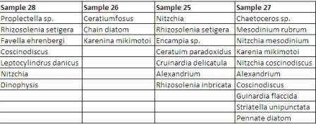
The phytoplankton samples taken from the offshore boat showed very few cells. There were 13 samples taken, and many were found to be empty after 10 transects had been taken. However, sample 7 was found to contain many Karenia mikimotoi cells, the highest value being 13 cells in one transect.


All the data on this website was calibrated to instruments aboard each of the research vessels.


Physical
From the data that was collected using the ADCP combined with CTD the Richardson Number was calculated. Around Lizard’s Point a Richardson’s number of less than 0.25 indicated a turbulent water column (Knauss, 2005). With increasing distance from the headland surface waters became laminar (fig.6.3) as frictional forces and shear reduced allowing a thermocline to develop. Between two distinctive water masses a front must occur at the boundary, which from our ADCP appears to occur at 1700m into the transect. A zooplankton bloom is evident here supporting this conclusion.
Bio-Chemical
Looking at the CTD data at station 2 (fig.6.7) it supports evidence for increased mixing, yielding relatively constant fluorescence, temperature and salinity throughout the water column. In contrast the offshore station 3 (fig.6.8) shows a distinct peak in fluorescence between 10 and 22m supporting the theory of nutrient entrainment across the thermocline within the euphotic zone(27m) allowing planktonic growth (Miller, 2005). The base of the thermocline coincides with the peak of fluorescence. Nutrient analysis (fig.6.9) gives an indication of nutrient availability within the water column. An oxygen peak at 12m (within the thermocline) also give evidence for production in this area. Nitrate and phosphate concentration have minima also at this point indicating uptake by organisms. However it is important to take into account that not all data supports this theory possibly due to sampling errors or other factors.
Helford Estuary
Comparing phosphate data (fig.6.10) between stations in the Helford estuary, concentrations increase with distance down the estuary, nitrate also follows a similar trend (fig.6.11). Silicon concentrations (fig.6.12) however show a reversed trend with a decrease in concentration down the estuary, this could be due to an imbalance in diatoms population distribution throughout the estuary. Oxygen saturations (fig.6.13) indicate an increase down the estuary possibly indicating a higher phytoplankton population in comparison to the mouth.
When comparing the data with data from the Fal estuary it can be seen that nutrient concentrations are higher in the Fal with mouth concentrations being greater by up to a factor of ten. Also within the Fal concentrations increase towards the river end whilst within the Helford estuary they increase towards the sea. This maybe due to inputs from agriculture, effluent or other factors. There also appears to be more zooplankton (fig.6.15 and 6.16) in the Helford estuary supporting the lower nutrient concentrations due to uptake. Greater euphotic zones with the Helford estuary (table)support the evidence further.
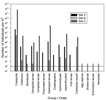
|
Site |
Location |
|
A |
Mouth of estuary |
|
B |
Upper estuary |
|
C |
Turnaware point |
The majority of zooplankton are found at turnaware point were the narrow upper estuary meets the main water body. Lowest levels were in the upper estuary. High levels at turnaware point could be explained by the influx of nutrients brought in from the river, while at the same time the salinity levels are close to that of the lower estuary. Lower levels in the upper estuary could be due to the slightly lower salinity levels or too further distance to migrate from coastal waters.
Copepods are the dominant group in the estuary and are found in large numbers at all locations. Gastropod larvae are found in high numbers at turnaware point, being the second most dominant group. However their numbers are much lower in the upper estuary. Despite copepods being the dominant group overall, their nauplii are only found further up the estuary, with very few at the mouth. This could be because the upper estuary is more nutrient rich and sheltered for the growth of the early life stages. Eggs and larval stages had the lowest numbers of all the zooplankton.
Phytoplankton were found in low numbers in all parts of the estuary. Rhizosolenia and Coscinodiscus appeared to be the dominant group of the few phytoplankton that were found. There does however appear to be quiet a diversity in the samples with a large variety of species found.

BMT Environment , 1994. An Environmental Review of the Fal Estuary and the Port of Falmouth : BMT Environment.
Gehrels W.R. 2010. ‘Late
Holocene land- and sea-level changes in the British Isles: implications
for future sea-level predictions’. Quaternary Science Reviews. Vol 29,
Issues 13-14, 1648-1660
Grasshoff, K., K. Kremling, and M. Ehrhardt. (1999). Methods of seawater analysis. 3rd ed. Wiley-VCH.
Johnson K. and Petty R.L.(1983) “Determination of nitrate and nitrite in seawater by flow injection analysis”. Limnology and Oceanography 28 1260-1266.
Knauss, J.A. 2005. Introduction to Physical Oceanography (2nd Edition). Waveland PR Inc. Pg 78, 253
Langston, W. J., Chesman, B. S., Burt, G. R., Hawkins, S. J., Readman, J., & Worsfold, P. (2003). Characterisation of European Marine Sites: The Fal and Helford. Maring Biological Association.
Loder, T.C., Reichard, R.P. 1981. The dynamics of conservative mixing in estuaries. Estuaries 4:1. P 64 – 69.
Miller, C.B. 2004. Biological Oceanography. Blackwell Publishing. Oxford. P 56 – 63
Morris,A.W., Bale, A.J., Howland, R.J.M. 1981. Nutrient distributions in an estuary: Evidence of chemical precipitation of dissolved silicate & phosphate. Estuarine, Coastal and shelf science. 12:12. P 205 – 216.
Parr, W., Wheeler, M., & Codling, I. (1999). Nutrient Status of the Glaslyn/Dwyryd, Mawwdach, and Dyfi estuaries - its context and ecological importance. WRc final report to the Countryside Council for Wales.
Parsons T. R. Maita Y. and Lalli C. (1984) “ A manual of chemical and biological methods for seawater analysis” 173 p. Pergamon.
JNCC. (2010). Fal and Helford - Special Area of Conservation - Habitats Directive. Retrieved July 1, 2010, from http://www.jncc.gov.uk/protectedsites/sacselection/sac.asp?EUcode=UK0013112
Centre of ecology and hydrology. http://www.nwl.ac.uk/in/nrfa/webdata/048003/g2008.html. Retrieved July 2, 2010
Over the time in Falmouth it was discovered that the estuarine and offshore zones behave differently creating different environments and conditions for plankton growth. Estuarine environments are mainly influenced by salinity, due to fresh water riverine inputs, causing haloclines, changing the conditions for plankton growth seasonally due to change in inputs. Phytoplankton within estuaries are often light limited, controlled by turbulence and suspended sediment in the water column. Offshore areas however are influenced primarily by temperature, which changes seasonally, causing the development of fronts and thermoclines and different conditions throughout the year for optimum primary and secondary production. Production in these areas are therefore greatly influenced by nutrient limitation, due to lack of input and reliance of remineralisation within the system.
Sediments in different marine habitats influences the marine biota inhabiting the area, due to their ability to live infaunally or epifaunally. Within the estuarine system, organisms can be influenced by the primary production on the sea bed such as kelp and maerl, whereas in the offshore area organisms are influenced by the primary production within the water column such as phytoplankton. The biology of the marine environment is dependant on both the chemical and geophysical properties of the ocean.