|
Falmouth Field Course: Group Four |
||
 |
General Aim: To gain a better understanding of the physical chemical and biological processes and properties of the Falmouth region. |
|
|
Falmouth Field Course: Group Four |
||
|
|
General Aim: To gain a better understanding of the physical chemical and biological processes and properties of the Falmouth region. |
|
.JPG) |
| Amy Astley |
| Rachel Boschen |
| Patrick Cooper |
| Esmé Flegg |
| Jack Maunder |
| Stephanie Moss |
| Simon Prissick |
| Adam Smith |
| Adam Sproson |
| Rebecca Summerfield |
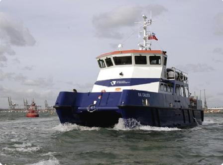 Fig. 2. Image of RV Callista |
RV Callista Specification:
Used for Offshore practical.
|
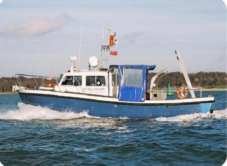 Fig. 3. Image of RV Bill Conway |
RV Bill Conway Specification:
Used for Estuary practical.
|
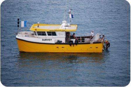 Fig. 4. Image of SV Xplorer |
SV Xplorer Specification:
Used for Geophysics practical.
|
| Equipment - Boat |
|
ADCP Implementation: The acoustic Doppler current profiler (ADCP) is a device which attaches to the hull of the research vessel and allows the user to analyse the movement of individual water layers, as well as the column as a whole. The device is often used to supplement and confirm tidal flow information taken from charts, as it can provide real time flow rate and direction. Description: The device operates by emitting a sonic ping which will reflect off suspended particles in the water, particles which are moving towards the receiver will produce a higher frequency and particles which are moving away from the receiver will produce a lower frequency; this is due to the Doppler shift, which the ADCP analyses and then produces a visual data plot on the movement of the water. By analysing and determining the Doppler shift on the seabed sound signature the ADCP can take into the account the movement of the vessel and therefore can be used whilst underway at slow speeds. Limitations: ADCP data becomes unusable when the vessel is travelling at speeds above 6 knots, however this value will be decreased in rough seas. In water exceeding 80m in depth the ADCP is unable to analyse the entirety of the water column. Data obtained by analysing the water layers in close proximity to the seabed can often give unreliable values due to contamination of the sound lobe as it comes into contact with the seabed; this is known as the sidelobe effect.
|
Fig. 9. Acoustic Doppler Current Profiler (ADCP) |
|
YSI probe Description: YSI is a multi-parameter probe that is capable of measuring, temperature, conductivity ( as a measure of salinity), pressure, dissolved oxygen, pH, chlorophyll and turbidity. It can store up to 49,000 sets of data and is accurate with a high resolution. Implementation: the probe is lowered into the water column giving continuous data out put at preset intervals, to a depth of 20m. This was used on RV Callista, during the offshore surveying. Limitations: must be calibrated to ensure accuracy. |
.JPG) .JPG) Fig. 10. YSI Probe
|
|
Video camera Description: A waterproof video camera which is mounted on a frame to stabilise the camera and its resulting footage. This was attached to the vessel by a electrical cable that is attached to the monitor aboard the vessel. It is used ensure the suitability of sediment prior to collection of samples via a Van Veen Grab, ensuring that there is no protected species e.g. sea grass and maerl and that the sea bed area is of suitable consistency i.e. not sea grass or hard rock. Implementation: The rig was lowered into the water by the crane and an image was shown on the screen. A video of the coverage was created. Limitations: Assume that the picture is representative of the entire area that is to be sampled. |
Fig. 11. Underwater Video Camera |
|
Plankton Nets I: Vertical plankton net Description: The mesh size of 200µm designed to retain plankton species >200µm in size, which are funnelled into a collecting vessel at the ‘cod end’. Aperture diameter of the net was 60cm. Implementation: Deployed from the vessel whilst on station to obtain a vertical sample of plankton between a specified depth and the surface. Using a brass messenger, the net can also be deployed to collect a fixed vertical plankton sample between two specified depths. Limitations: If the vessel is moving or drifting, the net may not remain vertical, meaning the distance travelled by the net may be greater than the exact vertical distance between the specified depth and the surface. Highly motile species may be able to escape the net. Organisms <200µm or >60cm in size will not be retained by the net. II: Bongo net Description: Two nets held together parallel, one with a 100µm mesh, the other with a 200µm mesh. Each mesh has a 60cm aperture diameter. Implementation: Deployed from the vessel whilst underway and towed at a speed <10kts. Larger plankton are retained both the 200µm mesh and the 100µm mesh, whereas plankton <200µm and >100µm in size are retained on the 100µm mesh.
|
Fig. 12. Closing Plankton Net
Fig. 13. Bongo Net |
|
Secchi Disc Description: The Secchi disc is a small circular metal plate attached to a notched rope so that it can be lowered into the water from a boat. The face of the disk is split into alternating black and white quadrants; this is to provide contrast when it is lowered into the water. Implementation: The Secchi disc is used to show light penetration and thus estimate the extent of the euphotic zone. Limitations: The major benefit of the Secchi disc is its simple usage but this is also its major constraint relying on personal opinion to give an estimate of the light penetration. |
Fig. 14. Secchi Disc |
|
Van Veen grab Description: The Van Veen grab is designed to collect a sample of bottom sediment, along with its associated biota. Implementation: It is deployed from a crane off the back of the vessel. The release mechanism is attached by chain to the hock and is deployed on hitting the seafloor. The impact frees the mechanism, causing the metre cubed box to cut into the sediment and once lifted to close around a sample of approximately 0.01 metres cubed. Viewing windows allow the sample to be observed from its original orientation before it is dumped into a tray for inspection. Limitations : The Van Veen grab can only be used in “blind sampling”, unless used in conjunction with the video camera. Some biota may be damaged in the process of grabbing, meaning that it cannot be used in sensitive areas such as beds of seagrass.
|
Fig. 15. Van Veen Grab |
|
Niskin Bottle Description: The Niskin bottle is a device for sampling seawater at specific depths. The Niskin bottle is an open ended bottle, with caps that can be snapped shut at specific depths trapping the water. The Niskin bottle is generally used in conjunction with a hydro line or multiple Niskin bottles can be attached to a CTD rosette allowing vertical profiles of a water column to be taken. Implementation: Five Niskin bottles used on the RV Callista with the CTD Rosette, where samples were taken depending on how mixed the water column is using information from the CTD Rosette, focusing on areas of interest, for example the thermocline. Limitations: The depth of a Niskin bottle can be inaccurate due to the line or CTD rosette not being completely vertical in the water column, and going down at an angle. Also in some cases the bottles can fail to close, which in many cases is only noticeable when the bottle has been retrieved, causing issues with time constrained projects. |
Fig.16. Niskin Bottles attached to a CTD Rosette |
|
Sidescan Sonar Description: This consists of a fish which is towed behind a boat, at a depth of 1m below the surface. The device emits two sound pulses simultaneously, giving a wide angled fan shaped beam. When the pulse reaches the seafloor it is reflected back, and this reflected pulse is measured. The degree of reflection depends on the density of the material and the slope of the sea floor. In some cases, shadow zones occur. These shadow zones are areas of no return pulse, and occur when a slope faces away from the beam. This helps to create a picture of the sea floor. Implementation: This device is used for mapping the sea bed, and to identify bathymetric features. It can be used in habitat mapping, by looking at the different sediment types on the sea floor. Limitations: The picture may be interfered with by movement in the water column. The results of this device are based on assumptions so it is also difficult to identify exactly what is present, unless supported by other equipment such as video footage. |
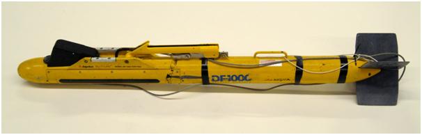 Fig. 17. Sidescan Sonar Towfish |
|
CTD Rosette Description: A CTD Rosette is a deployable metal frame used in conjunction with other instruments such as Niskin bottles (see above) and transmissometers to give a number of readings. Implementation: By using a winch or similar deployment technique the CTD rosette can be used to take a transect of the entire water column, also allowing water samples to be taken. Limitations: A CTD frame is a bulky piece of equipment which requires a strong winch system to allow deployment meaning smaller vessels may be unable to use such equipment. |
Fig. 18. CTD Rosette with attached Niskin Bottles
|
|
|
|
Fluorometer · Description: Flurometers are used to give an indication of chlorophyll levels and resultantly indicate phytoplankton concentrations. · Implementation: This results from stimulation of chlorophyll at the blue end of the light spectrum (oscillates between approximately 360-240nm, close to the UV end of the spectrum), with a response occurring from the red end of the spectrum (usually detected between 680-665nm). · Limitations: However if overstimulation occurs the chlorophyll will no longer occur. To prevent this a Pump Probe Fluorometer can be used which builds up the intensity of the stimulation to a saturation level.
|
Fig. 5. Image of a Fluorometer
|
|
Microscopes Description: Microscopes are an essential piece of laboratory equipment, allowing the user to see objects that are smaller than to be seen by the naked eye Implementation: Microscopes were used to count and classify and count the numbers of phytoplankton and zooplankton within our samples. Bugroff trays allow transects to be taken to provide a representation of the samples. Limitations: Microscopes rely on human input and so suffer from human error. As transects were conducted the counts won’t be fully accurate but a representation. |
Fig. 6. Image of Light Microscope |
|
Spectrophotometer Description: Is a type of photometer that measures intensity and wavelength of light. Implementation: Samples that have been reacted to produce a coloured product relative to the volume of nutrient being recorded, are place into the machine and a light is passed through the sample and the receiver the other side of the sample records the amount of light that has passed through and the wavelength of the light after passing through the sample. We used this to measure the nutrients (nitrogen, phosphate, silicon) levels in samples taken from the estuary and the offshore. Limitations: Other molecules present in the sample can also act as the wavelength under consideration and therefore cause an incorrectly high value. Limited to a certain range of the electromagnetic spectrum. |
Fig. 7. Image of Spectrophotometer |
|
Electronic Burette Description: Implementation: Limitations: |
Fig. 8. Image of Electronic Burette |
|
Overall Discussion At the top end of the river a large amount of mixing was shown on the ADCP. This area had a low Richardson number of 0.45, meaning there was high turbulence and particulate matter and resultantly low light available to the phytoplankton. This showed a transition between well mixed and stratified waters which could have been due to a slack in the tide. The estuarine environment was dominated by salinity, but there was little change between the upper and lower estuary despite a fresh water input at Turnerware Point. Towards Blackrock there is a transition to a more coastal system, where winds and tides dominated the structure and mixing regimes. There was also a transition between the salinity dominated structure of the estuary to the temperature controlled structure of the offshore region. The front was found between offshore stations 3 and 4, where there was a boundary between stratified waters and well mixed waters. There was a four layer system near the frontal region that had only been recently re-stratified indicating well mixed behaviour. In the offshore there was high light penetration compared to the estuarine waters where high particulate matter meant higher attenuation coefficient. At the top of the estuary a salt wedge system formed where fresher water overlaid a more saline and therefore denser water mass. This prevented mixing between the two layers; also the difference in ionic strengths between the layers caused the aggregation of particles increasing particulate matter and thus explaining the decreasing the light penetration. Silicon is pseudo-conservative element is this estuary, so there is uptake and renewal taking place at the same rate. Silicon is at low concentrations throughout the estuary and especially offshore. Phosphate is also at low concentrations throughout out due to uptake in the previous bloom; it is found at deeper depths in the offshore region. Nitrate peaks just below the surface due to remixing of nutrients after the spring bloom, and was undetectable towards the mouth of the. Nitrate concentrations were higher at the coast due to terrigenous inputs (e.g. station 2 offshore). Within the euphotic zone offshore nitrate levels were lower due to consumption by phytoplankton in previous blooms; whilst in the estuary, levels were lower except for station 2 (estuarine) where high concentrations were found due to eutrophication. Oxygen was found at very low concentrations at station 2 in the estuary. In deeper waters there are lower concentrations of oxygen due to a higher rate of respiration. Chlorophyll was fairly constant throughout all stations, and for the most part had a maximum at around 15-20m offshore. In the offshore chlorophyll concentrations were mostly uniform where the water column was well mixed, although some stations only had one sample. At station 2 (estuarine) there were high nutrient levels and very high chlorophyll levels, this indicated that the area was eutrophic. This is most likely due to inputs from moored vessels and effects concentrated by the shallow water and slow flows. High surface levels of oxygen and low concentrations of nutrients indicated a recent bloom of phytoplankton, yet the nets showed no evidence of phytoplankton. This can be explained by the large abundance of zooplankton throughout all samples both in offshore and estuarine environments. The diversity of the zooplankton was low with a dominance of copepods; this suggests that the copepods are out competing the other taxa of zooplankton. Another area in which the environment had a strong influence on species present was the biotopes of the Helford estuary, where the topography, chemical and physical environments played a part in the distribution of species. For example the anoxic muds to the north of the anchorage area and the coarse sands towards of the mouth of the estuary where the conditions favoured bivalves and polychaetes. The main limitations of this study were time and weather, which limited repetition of stations, so that only one tidal phase, weather condition and time period could be sampled. Human error was also an issue which occurred when recording latitude and longitude readings. Vessel capabilities were also a constraint as we could only sample to a certain depth, as we could not go to upper reaches of the estuary nor too far offshore. In the Helford estuary anthropogenic inhibitors such as the large areas of anchorage prevented a full side scan transect. Equipment resolution also posted a problem, for example the nitrate levels were at some points below the detectable limits of the equipment and so could not be sampled. Potential investigations included creating a full time series of each parameter at all locations, therefore overcoming the limitations of weather and providing the opportunity to sample throughout the yearly cycle. Also the use of more sensitive equipment so that all nutrients can be recorded even at low concentrations, meaning a full profile of the water column can be taken. Research boats with a shallow draft so that a vessel can go up the estuary or ribs could also be used to get a full transect of the estuary. Vessels with automated chemical analysis systems could allow more samples to be taken regularly so that a larger area can be surveyed in a smaller amount of time increasing efficiency.
|
|
Introduction Sampling was conducted on the South Coast of Cornwall in the Fal and Helford estuaries and offshore of Falmouth from Black Rock to Mounts Bay via Lizard Point and the Manacles. The Fal Estuary is a ria, or drowned river valley, that formed at the end of the last glaciation as a result of sea-level rise. This rise led to extensive wetlands in the upper estuary and in the deeper sections of the lower estuary, the formation of Carrick Roads, one of the largest natural harbours in the world (Langston et al, 2006). The River Fal, Helford River, River Carnon and Restronguet Creek all feed into Carrick Roads. The Fal estuary is macrotidal, with a mean tidal range of 5m and maximum tidal currents below 2 knots. The underlying geology is Carmellis granite and metamorphic rocks to the west. The catchment for the Fal Estuary has a long history of tin mining, resulting in substantial pollution of the water column and sediments, including the Wheal Jane incident in January of 1992 (Hunt and Howard (1994). There have been many pollution studies in the Carrick Roads area including those on heavy metal speciation and distribution (Williams et al, 1998; Pirrie et al, 2003) water quality (Neal et al, 2005) tolerance to copper (Burlinson and Lawrence, 2007) community response to pollution (Warwick, 2001) and imposex and intersex of molluscs as a results of TBT (Langston et al, 1994; 2007). The TBT concentration in the Fal estuary fails to comply with the European Quality Standard of 2ng l-1 (Langston et al, 2006). Despite their long history with mine pollution, the Fal and Helford portions of the estuary together form a European Marine Site (EMS) designated as a Special Area of Conservation (SAC) under the Habitat’s Directive. This designation recognises the importance of the area in having rare or endangered habitats or species. Habitats of interest in the SAC include Atlantic salt meadows, mudflats and sandflats exposed at low water, subtidal sandbanks and large shallow inlets and bays (Keddie, 1996). Other important habitats are the Zostera marina seagrass beds (Langston et al, 2006) and the mearl bed at St. Mawes bank, containing the most southerly living mearl in the UK and providing important habitats for a number of species (Farnham and Jephson, 1997). The Fal estuary has further interest as a result of blooms of the toxic dinoflagellate species Alexandrium minutum, which blooms in response to the high nitrate concentrations in the upper Fal estuary as a result of sewage treatment works in Falmouth and Truro and the run off from the agricultural land in the catchment area (Langston et al, 2006). Nitrates are so high in the upper Fal estuary as to designate it a Sensitive Area (Eutrophic) and Polluted Water (Eutrophic) under Nitrates Directive and Waste Water Treatment Directive respectively (Langston et al, 2006). In summer, the offshore environment can form a tidal front. Landward of the front, the water column is cooler and well mixed due to tidal and wind action. Salinity is also lower as a result of riverine input. Seawards of the front, the water column is stratified with a warmer surface layer and higher salinity. Where these two water bodies meet, a front forms, providing excellent conditions for phytoplankton species with high irradiance, a stable water column and access to nutrients below the thermocline. The blooms that result can be observed from satellite, indicating the location of the front (Le Fevre et al, 1983). |
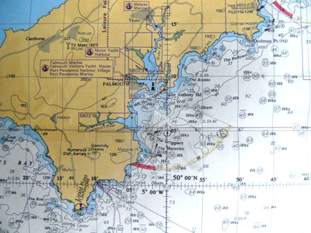 Fig. 1. Map to show location of sample sites, courtesy of Admiralty Charts |
|
Introduction A laboratory session was held to analyse all the water samples collected whilst aboard the RV Callista: plankton and zooplankton counts and identification; silicon, phosphate, nitrate, oxygen and chlorophyll analyses. The aims of such lab work are to prepare and analyse collected data allowing analysis and conclusions of the samples to be reached.
|
|
|
Method Safety note: A laboratory coat should be worn at all times whilst in the lab, legs and feet should be covered and no food or drink should be consumed. |
|
| Biological | |
|
Zooplankton Each sample of water collected on the previous day was initially treated with Formalin, before being stored in a fridge overnight. The samples were then shaken thoroughly to mix up the settled plankton. A small amount was decanted into a 25ml beaker, from which a 5ml sample was extracted, using a measuring cylinder. This was then transferred to a Bogorov chamber, which was viewed under a low power microscope. Each zooplankton was then categorised to at least phylum level with the use of an identification guide (reference )and recorded in a table. This process was repeated four times for each water sample. For those samples that contained a much higher concentration of zooplankton only a 2ml sample was taken. The values of zooplankton per 5ml and 2ml were then converted into units of metres cubed per sample. This volume could then be converted into metres cubed in the water column by dividing by the net volume taken (which is the area of the mouth multiplied by the length of the tow). |
|
|
Phytoplankton In order to quantify the number of phytoplankton present at a range of depths 100ml samples were taken from the Niskin bottles attached to the CTD profiler, these were then treated Lugol’s iodine in order to kill and fix the phytoplankton present they were then allowed to settle overnight. The sample was concentrated from 100ml down to 10ml using a vacuum pump to remove excess liquid, whilst be careful to avoid disturbing the fixed phytoplankton which has settled to the base of the tube. The concentrated solution was then transferred to a Sedgewitch-Rafter counting chamber using a pipette, the number of phytoplankton present were counted by performing 10 transects of the counting chamber under a microscope set to a magnification of x100. |
|
|
Chemical |
|
|
Silicon The samples for silicon analysis were refrigerated overnight in plastic containers. A pipette was first rinsed through with the sample before 5ml was then pipetted from each into a clean labelled tube. Three samples were randomly allocated to have replicates taken of them and were treated in the same manner as the other samples. To each of these tubes 2ml of Ammonium molybdate was added and the samples were allowed to stand for 10 minutes. A beaker for Mixed Reducing Reagent (MMR) was prepared using a measuring cylinder. The ratio was doubled in order to produce enough reagent for 3ml to be added to each sample. This contained 20ml Metol Sulphite, 12ml Oxalic Acid, 12ml Sulphuric acid (50% v/v) and 16ml MO water. Safety note: Whilst handling these chemicals gloves and safety glasses should be worn at all times. Especial care should be taken when decanting sulphuric acid. Once 3ml of the reagent had been added each tube was shaken and left for a minimum of 2 hours to develop. Silicon samples were analysed using a modified version of Mullin and Riley (1955), adapted by Parsons et al, (1984). A UNICAM 5625 UV/V15 Spectrometer was used to determine the absorbance of the silica samples at a wavelength of 810nm. The low silicon concentrations required a larger 4cm cell. Each sample was inverted to mix and introduced to the cuvette. The absorbance of the standards was plotted against their known concentrations to create a calibration curve used to determine the unknown silicon concentrations of the samples collected. The detection limit for silicon was 0.3µM.
Fig. 39. Offshore Silicon Calibration Plot
Fig.40. Estuarine Silicon Calibration Plot
|
|
|
Phosphate Calibration of phosphate standards Use a stock solution of 6 mili-molar phosphate which is exceedingly concentrated (X1000 of our samples) – so use a dilution process. Need to dilute by 400 fold to get a working solution. It is more effective to use a two step dilution process as otherwise the result would be a very large volume of sample – so prevents waste. Would not want to measure to a concentration of less than 100 microlitres. Must be very precise in measurements – most errors are random and result from inaccurate pipetting. Bottles used must also be clean and dry to prevent any inaccuracies or errors. Also any spillage of the stock solution could cause a contamination issue, especially as a result of its concentration. Best to measure from the stock solution when it is at room temperature – however in this case was used soon after removal from a refrigerator – minor issue of volume change. Initial dilution: Use 1ml stock solution and 99ml water (milliQ water) creating a 1 in 100 ratio of phosphate stock solution. Need to then mix the solution well to ensure any removal from the sample is representational of the true concentration. Secondary dilution: Transfer 25ml of the 1 in 100 phosphate solution into a 100m bottle; as usual must be very precise, and then fill with 75ml of miliQ water to create a 1 in 4 concentration. This is a 1 in 400 concentration compared to the stock solution. Calibrated samples concentration: 0.15µl, 0.3µl, 0.75µl, 1.5µl and 3µl standards and blanks. All samples have a total volume of 10ml. Create all standards in triplicate. Include two method blanks within sample (miliQ water and reagent). Replicate every 1 in 5 samples.
The samples were stores in brown bottles in a fridge, and were only removed when in use. Each bottle had a number inscribed on the side which corresponded to the numbers on the centrifuge tubes – into which a quantity of the samples would be placed. Three duplicate bottles (98, 111 and 104) were also going to be used to assess the accuracy of the pipette usage, resultantly judging humand random error – in theory the results for these duplicate bottles should be identical. A 5ml pipette was used to place a total of 10ml of sample into each centrifuge tubes. A separate 1ml pipette was later used to add 1ml of a pre-prepared reagent to the tubes. These samples were then left for a period of over 1.5 hours to allow the reaction to be completed before the analysis of the samples can begin. Contents of the mixed reagent in proportion: · 20% Ammonium Molybdate · 50% Sulphuric Acid (2.5 mole strength) · 20% Ascorbic Acid · 10% Potassium Antimonyl Tartrate Once the samples were fully reacted the 11ml solution was carefully poured into a 4cm glass cell and then their absorbancy was calculated by placing this into a spectrophotometer (Hiatchi model U-1800). To prevent errors the glass cell was placed in the same position for each analysis, by lining the edge of the cell up against the block . The outside of the cell had to be kept dry, as did the internal working area of the spectrophotometer. As the instrument had already been used by another group earlier in the day slight changes in calibration were avoided by ‘zero-ing’ against distilled water. For each sample two values were taken; whereas for the duplicates a total of 4 values were obtained. After each value was taken the solution was returned to the centrifuge tubes in case they were required at a later time. These data can then be used alongside the calibration curve using standards put together by another group (to allow more speedy work alongside the two groups).
Fig. 41. Offshore Phosphate Calibration Plot
Fig. 42. Estuarine Phosphate Calibration Plot
|
|
|
Nitrate The samples used for analysis were collected on Callista Prior to analysis the seawater was drawn up into a 5cm3 syringe and passed through a 13mm diameter PTFE filter with a 1µm pore size; this removes any particulate matter including phyto and zooplankton, this prevents blockages in the narrow diameter tubes. In order to analyse the nitrate content in the samples a flow injection technique was used, in which a flow of artificial seawater solution consisting of sodium chloride and ammonium chloride was sent through a series of pipes along with the reagents 0.1% NEDH and 1% sulphanilamide, this reacts with the nitrate present in the sample to produce an AZO dye. The flow through the tube is continuously monitored by a visual spectrometer which analyses light transmission, next the sample solution is introduced into the system in increments of roughly 1.5cm3. This is done using the injection component which momentarily diverts the flow of the artificial seawater, and injects a section of the sample solution into the flow. The flow then passes through the spectrometer and the chart recorder visually displays the change in light transmission. This was repeated for each bottle sample to allow identification of erroneous results and errors. The results of this nitrate analysis are displayed on the chart recorder trace where the peak heights are measured against a defined baseline. The sample concentrations can be calculated by drawing a calibration plot of the peak heights produced by running standard nitrate concentration of 1 µM, 5 µM and 10 µM; then by using the equation of the regression line the sample peak heights can be converted to concentrations. Equipment used - Flow injection system consisting of including spectrophotometer, chart recorder and sample injection component. Syringe (5cm3) PTFE Filter (13mm diameter, 1µm pore size) Reference - Johnson K. and Petty R.L.(1983) “Determination of nitrate and nitrite in seawater by flow injection analysis”. Limnology and Oceanography 28 1260-1266.
Fig. 43. Offshore Nitrate Calibration Plot
Fig. 44. Estuarine Nitrate Calibration Plot
|
|
|
Oxygen 1ml of manganese chloride and 1ml of alkaline iodide was added to a sample of seawater. These reagents were added in order to fix the oxygen in the sea water. This caused a precipitate of manganese iodide to be formed. The samples were left overnight. 1ml of sulphuric acid was the added in order to dissolve the precipitate. The sample was then mixed using a magnetic stirrer, until all of the precipitate had dissolved. This solution was then titrated with Sodium Thiosulphate, using an electronic burette. The end point of the titration was indicated by the solution becoming colourless. When the pen on the chart recorder levelled off, this indicated the end point. Equipment: Magnetic stirrer Pipette Beaker 665 Dosimat electronic burette Servoscribe 1s Chart recorder.
|
|
|
Chlorophyll A 50 ml sample was filtered through microfiber glass filter GF/F, of mesh size 200µm and 25mm diameter, the samples were stored in a fridge under acetone overnight. 6 ml were transferred into cuvette and left to settle to avoid the filter particles to affect the results. The Fluorometer was used to measure the sample chlorophyll level. Each sample was individually placed in the fluorometer and its fluorescence was averaged over a period of approximately ten seconds. Readings were presented in µmols, these were converted to µg/l. This was done by multiplying the value by the volume (6) and then dividing it by the amount of seawater filtered by the filter (50ml).
Fig. 45. Offshore Chlorophyll Calibration Plot
|
|
|
Results |
|
| Biological | |
|
Zooplankton During offshore sampling, zooplankton nets were deployed at every station (1-4), at various depths. At Station 1, the net was deployed and trawled between 20m at the surface. The dominant group of zooplankton here were copepods, with an estimate of 1682 individuals per m³, there were also low levels of copepod nauplii present. At Station 2, the net was deployed and trawled between 20m and the surface. Here the estimated average was 698 copepods per m³, and 115 nauplii per m³. At station 3 there were two nets deployed and trawled, one between 30 and 17 metres, and another between 10 metres and the surface. Here the deeper net found 306 copepods per m³ and 30 nauplii per m³. The shallower sample gave an estimated 7294 copepods per m³, it also had a higher copepod nauplii value than any other station at the shallower depth. At station 4 there were again two nets deployed and trawled. The first trawl we did was intended to be between 25m and the 13 metres, during this trawl the weight on the net was lost, meaning the trawl was in reality between 25m and the surface. The other trawl was between 13m and the surface, so in order to find the value of the 25-13m we subtracted the shallower trawl from the other trawl, this gave us very low levels of all plankton types. The shallower trawl gave higher plankton readings with estimated copepod numbers of 5298 per m³ and nauplii numbers of 88 per m³. We also trawled bongo nets, the results of this however are to be considered erroneous, and possibly an error due to the long length of time they were trawled for, with the nets reaching capacity after a certain point, meaning that after the calculations, the estimated values were no higher than 8 copepods per m³, which considering the location was chosen to find large amounts of plankton, is extremely low. Throughout all the stations, other plankton groups were found including Appendicularia, Echinoderm larvae, Ctenophora, Chaetognatha, Gastropod larvae, polychatae larvae, Decapoda larvae and Cladocera. The numbers of these organisms were consistently low throughout the stations rarely reaching higher than 30 per m³.
|
Fig. 46. Numbers and species of zooplankton found in net trawls
Fig. 47. Copepod (WoRMS (2010). Copepoda. Accessed through: World Register of Marine Species at http://www.marinespecies.org/aphia.php?p=taxdetails&id=1080 on 2010-07-09)
|
|
Phytoplankton Microscope transects showed a distinct lack of phytoplankton in the water samples, with very low numbers or organisms and a small range of species being observed. |
|
|
Chemical |
|
|
Silicon The silicon vertical profiles for station 3 showed a general decrease in silicon concentration with depth, whilst station 4 silicon vertical profile was variable with no observable pattern. Station 1 and 2 only had one data point available so no vertical silicon profile was obtained.
|
Fig. 48. Vertical Profile of Silicon Concentration for Offshore Stations
|
|
Phosphate At station one the concentration of phosphate at 10m appears comparatively high to stations 3 and 4, though this could be due to experimental errors at low concentrations. The concentration of phosphate at station 2 is the highest at any stations at a depth of 10m. Both these two stations were taken near to the shoreline, where the input of terrestrial phosphate will be less diluted than further offshore, which could explain their comparatively higher concentrations. The data from station 3 shows a peak of phosphate at 20 metres and two minima at 10 and 30 metres, though the difference between these two minima and maxima is only 0.002 μMolL-1. From 30 metres the phosphate decreases in the following two samples. This peak is likely to be due to analytical errors as it does not coincide with any other trends seen in the other nutrients. The phosphate concentrations for the forth station appear to follow a near linear trend, decreasing with depth. The maximum concentration is found at 5 metres of 0.004µMolL-1, decreasing to a minimum of 0.005µMoll-1 at 30 metres. The process of calibrating samples’ absorbance against the absorbance of standard concentrations has a limited sensitivity of 0.003μMolL-1. This restricts the values to which one can have confidence in, to those of concentrations above 0.003 μMolL-1. All the concentrations found were relatively close to 0.003μMolL-1 which is the limit of the equipment sensitivity this means one should be cautious when analysing this data. The range of concentrations is from 0.004 μMolL-1 (at stations 1, 3 and 4) to just 0.006 μMolL-1 (at station 3). |
Fig. 49. Vertical Profile of Phosphate Concentration for Offshore Stations
|
|
Nitrate Station 1 is located near Black Rock at the mouth of Falmouth estuary and has a relatively low nitrate concentration of approximately 0.5µmolL-1 at 10m. Station 2 is located roughly 2km off Lizard Point and has a relatively high nitrate concentration of approximately 5.2µmolL-1 at 20m. Station 3 is located roughly 5km south of Lizard Point. Nitrate concentrations decrease rapidly in surface waters down to 20m by approximately 4.5µmolL-1. Nitrate then increases between 20 and 75m by approximately 0.5µmolL-1. Station 4 is located a further 8km off Lizard Point then Station 3. Nitrate concentrations increase with depth by 0.7µmolL-1 until 20m where nitrate levels level out at 2.5µmolL-1.
|
Fig. 50. Vertical Profile of Nitrate Concentration for Offshore Stations
|
|
Oxygen Station 3 is located roughly 5km south of Lizard Point. Oxygen concentration and saturation follow a similar pattern, decreasing by approximately 15µmolL-1 and 10% respectively over 20m. Oxygen concentration and saturation then increase over the next 10m by approximately 4µmolL-1 and 1% respectively. Oxygen concentration and saturation decrease again after 13m by 20µmolL-1 and 11% respectively. Station 4 is located a further 8km of Lizard Point then Station 3. Oxygen concentration and saturation increase in surface waters down to 18m by approximately 20µmolL-1 and 5% respectively. This is followed by a sharp decrease in oxygen concentration and saturation over the next 2m by 50 µmolL-1 and 30% respectively. Oxygen concentration and saturation then decrease again over the next 5m by 5µmolL-1 and 1% respectively.
|
Fig. 51. Vertical Profile of Oxygen Concentration for Offshore Stations |
|
Chlorophyll Station 1 showed that the chlorophyll concentration within the seawater was at 1.069 µgL-1 at a depth of 2m. Chlorophyll concentration at station 2 (Lizard Point) was 0.7416 µgL-1 at a depth of 20m. Samples at station 3 showed a chlorophyll maximum at 20m whilst at station 4 the chlorophyll maximum was found at 15m. After the maximum in station 3 at 20m there was a steady decline in chlorophyll concentrations so that at 75m the chlorophyll concentration was 0.3936 µgL-1. In Station 4 there was a very rapid decrease in chlorophyll concentrations after the maximum, so that 5m deeper than the maximum (at 15m) the levels of chlorophyll were 0.4932 µgL-1.
|
Fig. 52. Vertical Profile of Chlorophyll Concentration for Offshore Stations
|
|
Discussion Few phytoplankton were found in analysis in comparison to zooplankton species, therefore it is likely that prior to sampling phytoplankton numbers were reduced as a result of zooplankton feasting on the phytoplankton species. It would be useful to get a clear picture of the bloom cycle timings within the Falmouth region to see if our prediction is indeed correct. Low silicon concentrations reflect that silicon requiring phytoplankton, such as diatoms, would have bloomed in spring, taking up all the available dissolved silicon. As the re-mineralisation process is slow and stratification of the water column prevents upwelling of fresh silicon from below the thermocline, the silicon concentrations in summer remain low. The higher concentration at depth reflects the slow remineralisation of siliceous phytoplankton species frustules at depth. Phosphate results were highest at station two and showed questionable results for the first station, which may be as a result of experimental error as the techniques for processing (i.e. filtering) of samples was only just being developed. This small range suggests that phosphate is not entering, or leaving, the system in large net quantities. The low level suggests a large uptake, which could be due to a previous phytoplankton bloom (though no evidence was found in the phytoplankton count of this). One would expect station four to have the lowest concentrations of phosphate at the surface due to its high level of stratification and so the prevention of mixing, thus over time phosphate will be taken up by phytoplankton and not as readily recycled into the surface layers. This can be seen in station fours results as it has the lowest surface concentration of any station.This small range suggests that phosphate is not entering, or leaving, the system in large net quantities. The low level suggests a large uptake, which could be due to a previous phytoplankton bloom. For chlorophyll results stations 1 and 2 were single data points as the water column at these positions was found to be very mixed (reference to CTD). The difference in the depths (5m) of the chlorophyll maximums at stations 3 and 4 could be due to the zooplankton being higher in the water column at station 4. Also the very rapid decrease in chlorophyll at station 4 could be due to a bigger population of zooplankton being present (refer to zooplankton data). Station 3 is the only profile in this data set that shows the changes within the water column. This was an interesting station as the water had been recently re-stratified into a four layer system hence why a profile could be made. The reasons less samples were taken at station 4 was that it was near the front and so the top 20m was stratified but below 20m the water was well mixed. Station 4’s position near the front would explain the larger population of zooplankton and therefore the higher chlorophyll maximum. At Station 3 the peak of Oxygen at 10m is associated with an increased level of phytoplankton activity, due to the presence of a strong thermocline. At depths below this zooplankton levels are increased producing higher levels of respiration than photosynthesis, and so oxygen is consumed. At Station 4 there is strong thermocline which constrains the phytoplankton bloom to the surface 17, creating a large maxima oxygen at this depth. Below which respiring zooplankton have taken up the oxygen in great amounts, producing an even great oxygen minima. Station 1 nitrate has been taken up in large amount by a recent bloom in phytoplankton. At Station 2 relatively high levels of nitrate are present due to terrigenous input and high mixing recycling nitrate from cold bottom waters. Station 3 nitrate is used up in surface waters by phytoplankton, which are confined to the euphotic zone which is defined by the thermocline at 20m. Nitrate is present in higher concentrations in bottom waters due to low vertical mixing, preventing nitrate from being re-introduced into surface waters. At station 4 nitrate is being used up in surface waters by phytoplankton, which are confined to the euphotic zone which is defined by the thermocline at 20m. |
|
|
Fig. 19. Google Earth Offshore Location Map
|
Aims: To study ADCP data to attempt to observe the position of
the front, and also to analyse the biological structure of organisms
found at the sample locations. Planning: After reviewing the previous groups’ chart plots. It was decided that samples would be taken to the South West of Falmouth. This was due to the lack of significant change in the tidal regime between the two offshore data collection days and so provides a larger range of data over the period of the field course. As the data was going to be collected offshore in potentially rough waters Callista would be the research vessel used; this is due to its stability and its onboard laboratory capabilities. Given the time constraints the plan was to measure at four stations with the possibilities of doing other locations and repeat readings if time permitted. Introduction: RV Callista was taken to 5 stations off the coast of Falmouth on 30th June 2010 between 08:00 and 16:00 GMT, the vessel left Falmouth harbour was taken to 5 stations off the coast. The first station was situated at Black Rock, at the mouth of the Fal estuary. The second station was situated at Lizards Point, a headland to the west of Black Rock. The stations that followed were located offshore, to the south of this headland, at increasing distances from the coast. For exact position coordinates see “Boatwork” The instruments used aboard Callista were:
At each station the CTD with rosette frame was deployed, which provided data on the vertical profile of temperature, salinity and fluorescence along with light data. This gave an indication of the structure and features of the water column. The rosette helds several 5 litre Niskin bottles which were used to take ‘in situ’ water samples at each station. The number of samples at each station, and the specific depths chosen depended on the structure of the water column. Additional information was collected using a plankton net of 60cm diameter and 200micron mesh size. At station 1, at Black Rock, the CTD results showed a homogenous water column. Therefore only one sample was taken at 10 meters using the Niskin bottle because the properties of the water did not vary with depth, when CTD profile was assessed. The Acoustic Doppler Current Profiler was also used at each station. This provided information on currents, shear within the water column and the presence of particles. A vertical plankton net sampled from the bottom (18m) to the surface of the water column to ensure the equipment was in working order. CTD data at station 2, Lizards Point, also showed a homogeneous water column. One water sample was also taken at this station, at 20m. A vertical plankton net was also deployed which sampled from 20m to the surface, in order to analyse the plankton in the euphotic zone. At station 3, the CTD measurements were taken and the vertical profile analysed. The water column indicated stratification at this station. This resulted in the decision to take five samples at various depths in order to attempt to capture the differing conditions throughout the water column. The vertical plankton net was also used at this station, with samples being taken from 30-17m, and between 10m and the surface. These ranges were chosen to reveal the effect of the thermocline on the numbers of plankton and abundance of certain species. At station 4, CTD results were supplemented by four samples taken through the water column, at depths chosen using similar criteria to station 3. The CTD data showed a stronger stratification, and a very distinct chlorophyll maximum within the water column. Two depth ranges were sampled using the vertical plankton net, in order to capture the variations at this maximum, and around it. Plankton samples were taken from 30-17m, and 10m to the surface. In addition to rosette sampling and CTD data, measurements of the current, shear in the water column, and backscatter due to particles in the water column were also recorded using the hull mounted Acoustic Doppler Current Profiler. Measurements of light penetration and turbidity were obtained by deployment of a Secchi Disc were taken at each station. A horizontal transect was also taken at each station in order to investigate the reason for the well mixed area at station 2. For horizontal transects, ADCP measurements were taken, to help analyse any internal mixing which may be taking place. Through out this experiment, underway temperature measurements were taken using water from the onboard pump and a temperature/salinity probe. This was aimed at detecting the ‘front’ that was located to the west of Falmouth in offshore waters. A Bongo net was also deployed, and a sample taken along a horizontal transect located in an area where a front was indicated i.e. between station 3 and 4. The Bongo net consisted of two adjacent nets, each 60cm in diameter. One net has a 200mircon mesh size, and the other has a 100micron mesh size.
|
|
Station 1 Conditions and Other Information: Cloud Cover: 8/8 octants Latitude 50° 08.107N Longitude 005° 01.537W Time 08:34.27GMT Water Depth 16.9m |
|
|
Station 2 Conditions and Other Information: Cloud Cover: 7/8 octants Latitude 49° 55.470N Longitude 005° 11.762W Time 10:13.27GMT Water Depth 71.4m |
|
|
Station 3 Conditions and Other Information: Cloud Cover: 3/8 octants Latitude 49° 54.000N Longitude 005° 13.39W Time 11:06GMT Water Depth 79m |
|
|
Station 4 Conditions and Other Information: Cloud Cover: 4/8 octants Latitude 49° 50.34N Longitude 005° 12.64W Time 12:14GMT Water Depth 33m |
|
|
Station 5 Conditions and Other Information: Cloud Cover: 4/8 octants Latitude 49° 52.98N Longitude 005° 13.55W Time 13:08GMT Water Depth 33m |
|
|
Other Measurements Information: Location: The Manacles |
|
Fig. 96. Google Earth Image of the Helford Estuary Survey
|
Aims:
To complete a total of three transects, and then use the available data to complete a number of grabs at sites which look interesting in nature. Planning: The night before working on the Xplorer a discussion was held on where would be best for studies to take place. It was decided that the top end of the Helford estuary would be a suitable location. Introduction: General History The Helford estuary is a Ria (drowned river valley) that was formed 10,000 years ago when the last glaciers retreated. It is situated on the eastern side of The Lizard Peninsula. The land closest to the river is surrounded by ancient deciduous woodlands, but historically the catchment area was dominated by agriculture and large load bearing quays, whilst river was used as a passage way for the products of the mining and granite industry. Heavy usage increased siltation of the creeks and eventually the estuary (Millward and Robinson, 1971). In the 20th century the mining industry’s collapsed and was replaced by leisure and tourism so that the Helford is an area for pleasure crafts and holiday makers. The maritime climate, sheltered nature of the area, the variation in soil type, depth and fertility has meant there is a wide variety of farming activities from arable to cattle farming (Reynolds, 2000)making the Helford an important agricultural area. Habitats The Helford estuary has a mild climate throughout the year and is sheltered from westerly winds, creating numerous habitats and acting as an important refuge for winter migrants. There are five distinct habitats found in the Helford. Sand and shingle shores are home to tube and peacock worms, sea slugs and cockles. The mudflats (found in the upper creeks) are rich in nutrients and are abundant in invertebrates, attracting migratory birds. Rocky shores are found at the mouth of the estuary (Rosemullion Head) and along the Helford Passage. The rocky shores are home to starfish, sea urchins, sponges, crustaceans and the Trumpet anemone one of the scarcest species of anemones in the UK. Kelp forests are also found on the lower shores, their holdfasts supporting a community that includes the rare fish, Couch’s Goby. Off Durgan and Grebe eelgrass beds are found, eelgrass is the only British flowering sea plant, where they are currently under threat by anchorages of the pleasure boats. This has caused the local sea horse population to disappear. Another important habitat in the Helford is the maerl bed that is situated at St. Mawes Bank (http://www.helfordmarineconservation.co.uk/helford-habitats.htm). Conservation The Helford estuary is a unique area that consists of many different habitats. Due to the sheltered nature of the area it is an important nursery for juvenile fish, molluscs and crustaceans. There is little freshwater input and the water column is well mixed with very little variation in salinity, unless there is heavy rainfall in the upper creeks. In 1987 it became a Voluntary Marine Conservation Area (VMCA). In recent years it has become a Special Area of Conservation (SAC), SSSI (at the mouth Rosemullions Head) and an Area of Outstanding Natural Beauty (National Park), recognising the importance of the area as supporting important species such as Fan mussels, maerl. To monitor the area it is being surveyed to define biotopes, recording current communities so that changes can be noted and if need be stopped (http://www.helfordmarineconservation.co.uk/conservation.htm). The Helford estuary was surveyed on 3rd July 2010 between 08:00 and 15:00 GMT. The aim was to identify and define a range of biotopes in the area, to use grab samples to ground truth the side scan sonar data and to use a variety of instruments (sector scanner, ADCP and Van Veen grab), to survey the bathymetry of the Helford estuary. Three transects over two locations were completed as well as 4 grab samples within these transects at points of interest that were observed on the side scan trace. Methods used for each transect: A sidescan trace was taken for transects 1, SG6 and SG5, with two grab samples taking place at the first transect and one grab for the other two. Sector scanner and ADCP data were taken during each transect. However the video camera was only successfully deployed and used during a grab on transect SG5.
|
||||||||||||||
|
Saturday July 3rd
Spring Tides |
|||||||||||||||
|
Transect 1 Information: Latitude 50° 05.410N to 50° 05.5994N Longitude 005° 10.6541W to 005°08.7145W Time 09:28.58GMT to 09:47.32GMT
|
|||||||||||||||
|
Transect SG6 Information: Latitude 50° 05.8699N to 50° 05.8685N Longitude 005° 06.2489W to 005°07.1874W Time 09:28.58GMT to 09:45.17GMT
|
|||||||||||||||
|
Transect SG5 Information: Latitude 50° 05.8922N to 50° 05.8951N Longitude 005° 07.1695W to 005°06.3927W Time 11:47.33GMT to 11:53.24GMT
|
|
Method The Helford River was surveyed on the 3rd of July 2010 using the vessel RV Xplorer. Time of departure was 07:00 GMT returning at 13:30 GMT. The speed of the vessel was approximately 20knots. The travelling time from the dock to the Helford was an approximately hour and a half, the first ADCP data set was started at 09:27 GMT. The exercise aimed to investigate benthic habitats in the River Helford and to show the main geophysical features and seabed types in order to answer questions related to biotopes. The equipment for this investigation was a side-scan sonar, an Acoustic Doppler Current Profiler (ADCP), a Van der Veen grab sampler and video equipment. RV Xplorer towed the side scan sonar device along a predetermined track. A busy anchorage in the middle of the estuary both restricted and determined the track plotted. The track was recorded and displayed by a program supplied by Trimble, called Hydropro. The average speed of Xplorer for each transect is shown in the table below. In total three transects were taken, full details of the latitude and longitude along with start times GMT are located in the results section. The side scan sonar produced an image of the seabed with a 75 meter swath either side. Intensity variations of the backscatter shown on the image provided information on differences in substratum on the sea bed. Areas of particular interest were chosen for grab sampling by studying the paper trace. The side scan images were used to confirm the bottom types. The initial intention had been to use a camera to view the biota prior to sampling. As the sonar “fish” was towed along the transect, positional data was recorded every 2 minutes in the log book. Whilst recording the side scan trace, the external environment was monitored for disturbance and the position of any potential interference was noted. Key features were also marked onto the edges of the trace plot coming out of the Thermo printer. Areas of particular interest were chosen for grab sampling by studying the paper trace. The ADCP was used to give a visualisation of the current velocity bathymetry of the Halford estuary. The data were displayed and recorded in WinRiver for later analysis. The Van Veen Grab samples were sieved in a sieve stack on the back deck. Sediments were classified according to grain size. Living or dead organic material was identified and recorded in the log book. Photographic data was collected to enable species identification. All grab samples collected were replaced in the area they were collected from to minimise any alien species transfer. Two transects were completed in the mouth of the estuary, this time constrained by local industry (oyster pots) sampling the edge of a depression with a depth of 9 meters, to see the possible changes in the biotopes of the area. |
||||||||||||||||||||||||||||||||||||||||||||||||||||||||||||||||||||||||||||||||||||||||||||||||||||||||||||||||||||||||||||||||||||||||
| Sidescan | ||||||||||||||||||||||||||||||||||||||||||||||||||||||||||||||||||||||||||||||||||||||||||||||||||||||||||||||||||||||||||||||||||||||||
|
The Sidescan sonar equipment was used as a tool to determine sea bed substrate types as well as the general positioning of other features e.g. oyster beds. Using this type of data the sidescan trace will then be used as a guide to assist in the decisions on the locations of points at which grabs and video footage might be taken. Features and structures can also be determined from a sidescan trace as a result of differences in reflection and absorption of the energy from the sonar emission. |
||||||||||||||||||||||||||||||||||||||||||||||||||||||||||||||||||||||||||||||||||||||||||||||||||||||||||||||||||||||||||||||||||||||||
|
Aims To effectively use sidescan data to locate the position of substrate changes as well as a dip in substrate level surface within the Helford estuary. Data collected will hopefully be clear enough to allow identification of bedforms such as ripples if present in the region studied. |
||||||||||||||||||||||||||||||||||||||||||||||||||||||||||||||||||||||||||||||||||||||||||||||||||||||||||||||||||||||||||||||||||||||||
|
Grabs |
||||||||||||||||||||||||||||||||||||||||||||||||||||||||||||||||||||||||||||||||||||||||||||||||||||||||||||||||||||||||||||||||||||||||
|
Grab One Sediment Properties: The sediment was very anoxic, with no visible oxic layer. Estimated sediment classification of mud, very dark grey in colour with high levels of organics. No living organisms were found within the sample. Flora and Fauna:
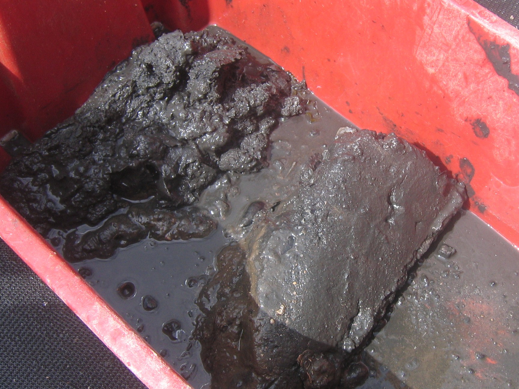
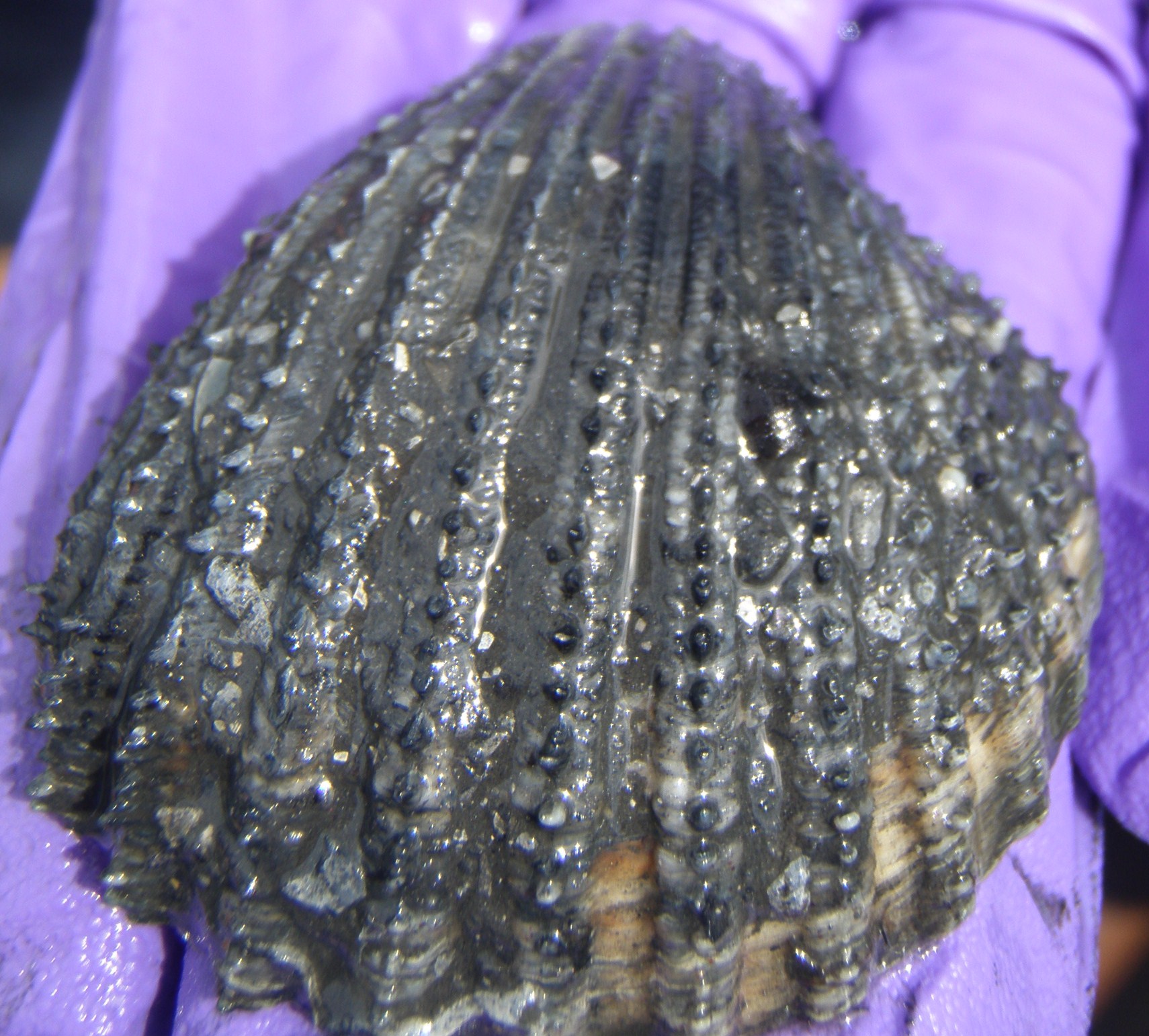 Fig. 97.Sediment sample from grab Fig. 98.Spiny cockle shells (Acanthocardia aculeate) |
Latitude: 50° 05.5616N Longitude: 5° 09.7338W Time: 10:20:34 GMT Depth: 3.7m |
|||||||||||||||||||||||||||||||||||||||||||||||||||||||||||||||||||||||||||||||||||||||||||||||||||||||||||||||||||||||||||||||||||||||
|
Grab Two Sediment Properties: The sediment had an estimated 2-3mm surface oxic layer but no living organisms were found in the sample. The sediment was sandy mud. Flora and Fauna:
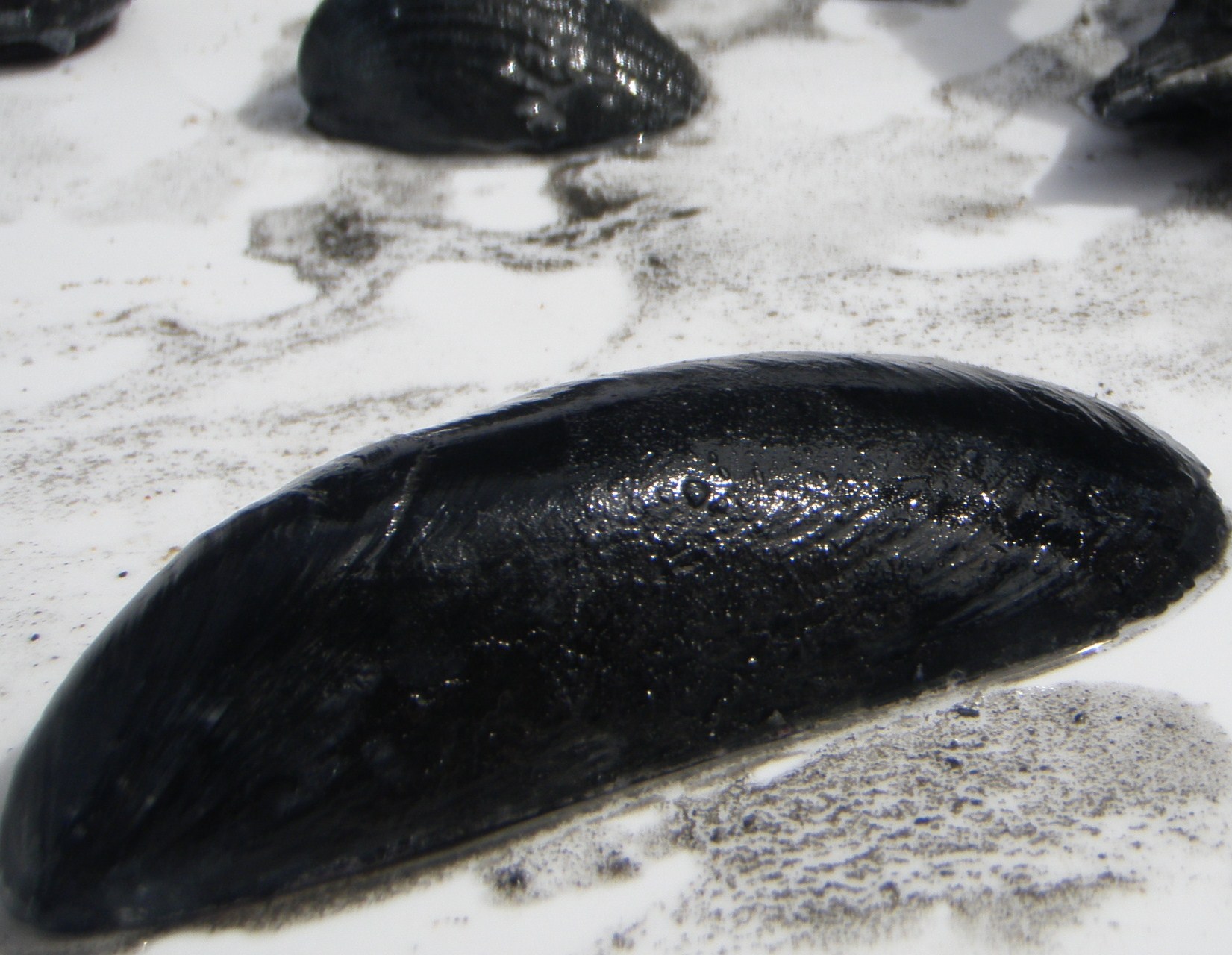
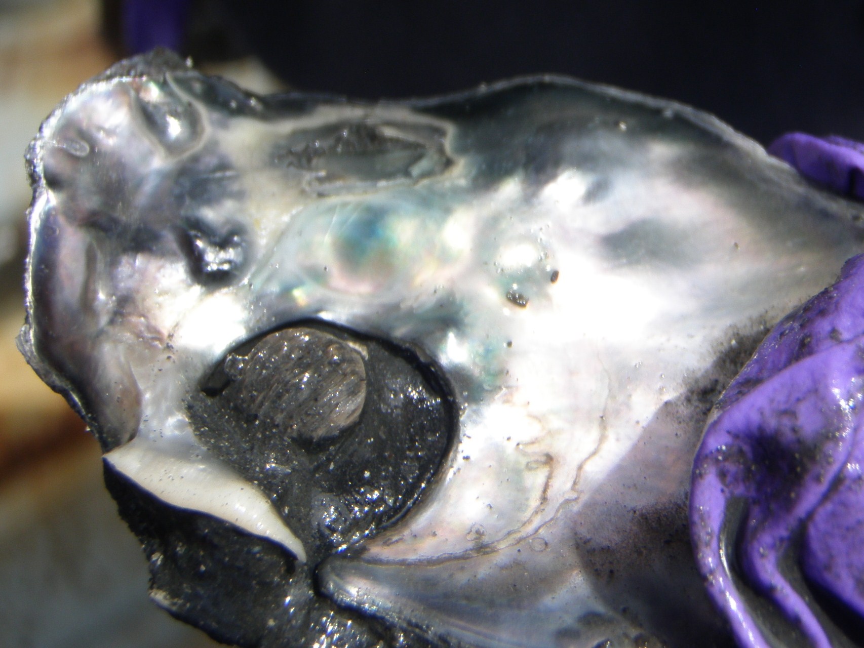 Fig. 99. Common mussle shell (Mytilus edulis) Fig. 100. Common oyster shell (Ostrea edulis) |
Latitude: 50° 05.7004N Longitude: 5° 09.1607W Time: 10:47:59 GMT Depth: 5.2m |
|||||||||||||||||||||||||||||||||||||||||||||||||||||||||||||||||||||||||||||||||||||||||||||||||||||||||||||||||||||||||||||||||||||||
|
Grab Three Sediment Properties: The grab sample consisted of mixed seaweeds (red, brown and green) along with the sediment. Within the sediment there were numerous small shell fragments, which some seaweeds had attached to which some seaweed species attached via their hold-fast. Flora and Fauna:
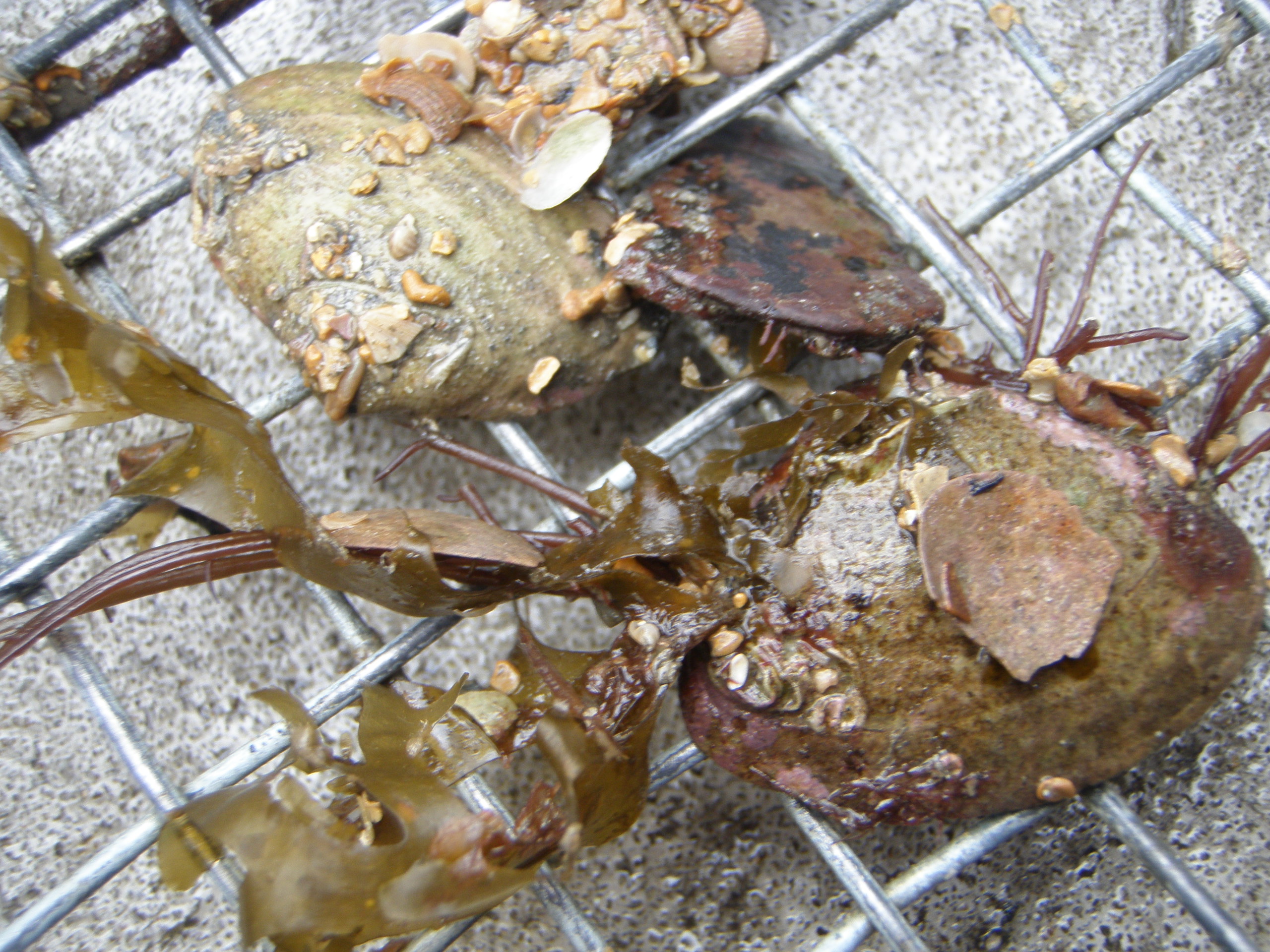
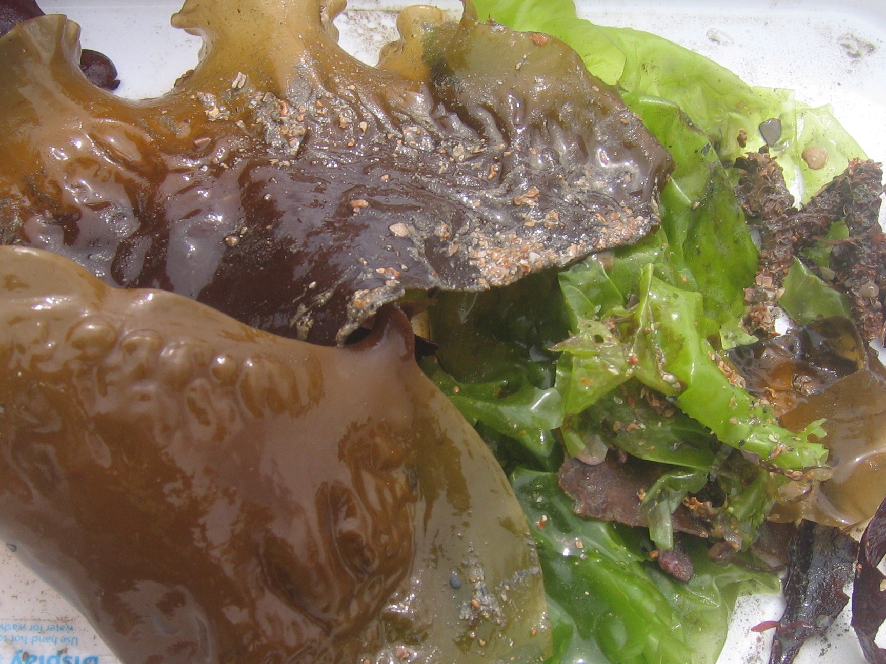 Fig. 101. Cockle and other bivalve shells Fig. 102.Mixed seaweeds (red, brown and green) |
Latitude: 50° 05.8991N Longitude: 5° 06.6489W Time: 12:05:07 GMT Depth: 7m |
|||||||||||||||||||||||||||||||||||||||||||||||||||||||||||||||||||||||||||||||||||||||||||||||||||||||||||||||||||||||||||||||||||||||
|
Grab Four Sediment Properties: The material sampled mainly comprised of small shell fragments and some coarse sand. This grab was the only one where living fauna were found. Fauna and flora:
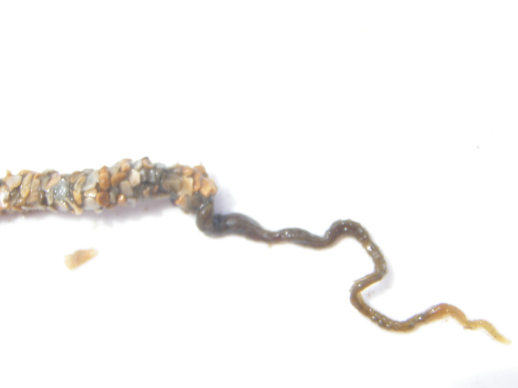
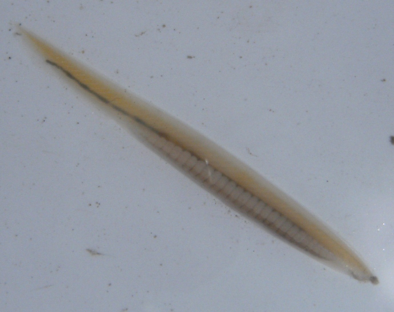 Fig. 103. Sand mason worm (tubes and polychaete) Fig. 104. Amphioxus (Branchiostoma sp.) |
Latitude: 50° 05.8721N Longitude: 5° 06.5611W Time: 12:28:09 GMT Depth: 7.1m |
|||||||||||||||||||||||||||||||||||||||||||||||||||||||||||||||||||||||||||||||||||||||||||||||||||||||||||||||||||||||||||||||||||||||
|
Video The video system was only deployed successfully at Transect Two, Station Two as earlier attempts during Transect One found the water too cloudy with sediment particles. It was possible that as the water was fairly shallow at these sites the movement of the Xplorer’s motors may have disturbed the surface sediments. The lens of the video was also shown to be slightly fuzzy, likely as a result of the instrument becoming too warm. Measures were then carried out to cool the lens for a period of time, to see if this helped to improve picture quality. A successful video deployment occurred during observation at Transect Two, Station Two, as the water was deeper and resultantly less murky; and also as the lens had been cooled. Organisms which could be identified directly from live footage included a number of seaweed species (broadly classified as red, brown and green species), small shells and a substrate of fine shell segments.
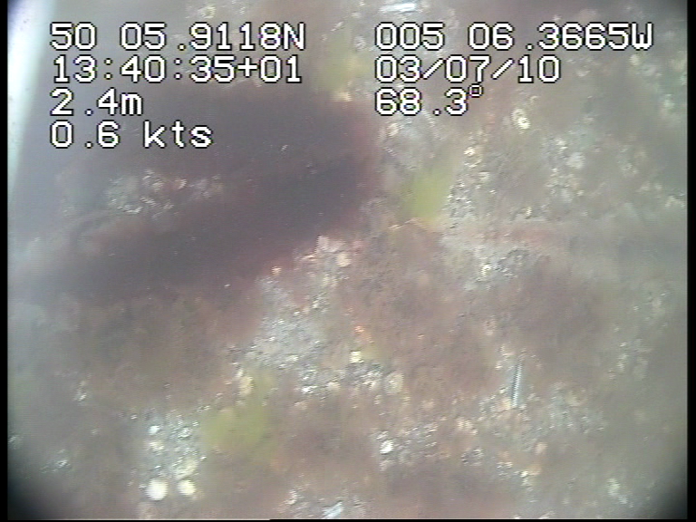 Fig. 105. Video Camera Image
|
||||||||||||||||||||||||||||||||||||||||||||||||||||||||||||||||||||||||||||||||||||||||||||||||||||||||||||||||||||||||||||||||||||||||
| ADCP | ||||||||||||||||||||||||||||||||||||||||||||||||||||||||||||||||||||||||||||||||||||||||||||||||||||||||||||||||||||||||||||||||||||||||
|
The GPS co-ordinates for starting and ending of the ADCP files were taken from the video monitor. After comparing them with those from the Nav plot it was noted that the two did not match. Therefore when dealing with the ADCP data the times used were from the ‘winriver’ file, from which the location could be determined. |
||||||||||||||||||||||||||||||||||||||||||||||||||||||||||||||||||||||||||||||||||||||||||||||||||||||||||||||||||||||||||||||||||||||||
Transects 1 to 4 follow the path of the initial sidescan plot along the Helford River towards the anchorage site. All four plots indicate a sporadic, although low, velocity magnitude and direction over the entire depth and course of the path. The average velocity increases downstream from 0.04m/s to 0.07m/s, coinciding with the increase in depth .
Profiles 8 to 10, from the mouth of the Helford estuary, transect SG6, indicate two layers of flow within the water column. The surface flow from 0m to 3m has a greater velocity than that of the one below and is flowing in an Easterly, direction towards the mouth. The lower layer from 3m to the seabed is approximately 0.1m/s slower and follows a more Southerly direction. In the third profile this directional change does not occur, though there still appears to be two very distinct layers of velocity magnitude.
The ADCP profiles of the second transect in the mouth of the Helford estuary, transect SG5, still show a distinct faster surface layer with an Easterly direction. The lower layer of flow however has no obvious dominant direction, unlike transect SG6. Discussion Transect 1: The low variable velocities of the first transect is likely to be due to the changing of the tides at approximately this time from flooding to ebbing flow, causing conflicting flows at this station. The topography appears to be one of the main influencing factors of velocity magnitude and direction, shown by the change with depth along the track. These fluctuating parameters are likely to inhibit the formation of discrete bedforms. The increasing velocity downstream makes it more likely that if bedforms did occur they would form downstream, towards the end nearest the main area of anchorage. On the first sidescan transect two discrete areas of bedforms were identified. The velocity magnitude and direction appear similar to the rest of the transect at these points, with the only difference seen at these locations being the water depth. Both areas of bedforms were found in significantly deeper water, but it is unclear as to whether it was the change in depth that resulted in bedform formation, or that the bedforms created the change in depth by erosion. This could only be established with more information on the type or the bedforms and their duration. Transect SG6: The more regular flow found across the ADCP files of transect SG6 would be more likely to instigate distinct bedforms along this stretch of the Helford estuary compared to station 1, though the formation of bedforms is dependent on the sediment type at the station, which was found to be mostly made up of coarse shell pieces, so the area is unlikely to support the formation of bedforms. Transect SG5: The ADCP profiles making up transect SG5 indicate that the area covered is less likely to support the formation distinct bedforms as the lower layer has no dominant direction and so there would be insufficient time of flow in one direction for bedforms to form. |
Fig. 106. Image from station 1
Fig. 107. Image from station 1
Fig. 108. Image from station SG6
Fig. 109. Image from station SG6
Fig. 110. Image from station SG5
Fig. 111 Image from station SG5
|
|||||||||||||||||||||||||||||||||||||||||||||||||||||||||||||||||||||||||||||||||||||||||||||||||||||||||||||||||||||||||||||||||||||||
|
Sector Scanner |
||||||||||||||||||||||||||||||||||||||||||||||||||||||||||||||||||||||||||||||||||||||||||||||||||||||||||||||||||||||||||||||||||||||||
|
An active sector scanning profiler was used to help describe the composition of the substrate in conjunction with the sidescanning profiler. It works by emitting sound pulses from a transducer and with the use of a hydrophone listens for the echoes (www.furunousa.com/productDocuments/CH37.pdf). The sector scanner was aligned to scan a vertical-fan passing through the water column below. This was restricted to 45° either side of the vertical profile. This allows for a small distance either side of the boats track to be viewed. However, towards the edges of the scan the beam will become stretched and so will no longer give a true picture. The intensity of the reflection depends on the composition of the substrate and can help to describe features found on the sidescan profile. Any images on the scan found below the seabed line will be disregarded, as the frequency used cannot penetrate through the seabed and these signatures are as a result of noise disturbance in the system.
|
Fig. 112. Sector Scanning Readout |
|||||||||||||||||||||||||||||||||||||||||||||||||||||||||||||||||||||||||||||||||||||||||||||||||||||||||||||||||||||||||||||||||||||||
|
At 0940 GMT the thickness of the seabed sounding decreases significantly in comparison to the previous recordings, suggesting a change in substratum. By relating this time to the sidescan it’s possible to find the position at which this occurs. At this point on the sidescan the trace becomes whiter, as there is a decrease in backscatter, indicating the sediment has indeed become finer.
|
Fig. 113. Sector Scanner Readout
|
|||||||||||||||||||||||||||||||||||||||||||||||||||||||||||||||||||||||||||||||||||||||||||||||||||||||||||||||||||||||||||||||||||||||
|
Discussion The sidescan data collected clearly showed areas of changing substrate composition moving downstream towards the estuary mouth ranging from muddy sand to shell fragments giving an indication of oxygen saturation, flow speeds and even organisms existing in the region. This data also showed the position of bedform features such as ripples and sand waves, which are thought to exist in regions of faster flow, and so also giving an indication of flow speeds. However insufficient data was available to decide whether the features were ephemeral as a result of tidal influences or had a more permanent presence. The sector scanner was used to back up sidescan data, giving indications on sediment type change. Grab data from four sites were used to give an indication of the benthic environment. Observations were made on sediment type and (if relevant) the depth of the oxic layer as well as the presence of fauna and flora (notes were also made as to whether they were living or dead). This data showed that more favourable environments existed towards the direction of the estuary mouth compared with the riverine end, with the only living fauna identified at grab site four. Such data gives a clear view on how estuarine environments are variable across fairly small distances, indicating how tolerant species present must be. Taking into account the sediment type, direction and strength of flow it is unlikely that any of the stations would support large areas of distinct bedforms at the time of surveying. This is not to say that localised bedforms might not occur, as the ADCP and sidescan only take into account changes in large areas, so there might still be small pockets of different sediment types and flow that the instrument could not detect. The Helford estuary is also a continually changing environment and so the results found can only be applied to the time and conditions from when the results were taken. |
||||||||||||||||||||||||||||||||||||||||||||||||||||||||||||||||||||||||||||||||||||||||||||||||||||||||||||||||||||||||||||||||||||||||
| Transects |
|
CTD Station 1, located at Black Rock is found just outside the mouth of the Falmouth estuary. There is a relatively small thermocline at 10m of about 0.6oC, which coincides with maxima in fluorescence at approximately 12m indicating a high abundance of phytoplankton at the thermocline. We also see a relatively small increase in salinity with depth. At Station 2 temperature decreases with depth but no thermocline is present. Salinity remains relatively constant with depth, indicating a well mixed water column. Fluorescence increases in a linear fashion with depth until approximately 10m and then remains relatively constant at approximately 0.16 after 10m. Station 3 shows a large decrease in temperature with depth, with a strong thermocline at 10m, where temperature remains relatively constant for 20m. This coincides with fluorescence maxima at 20m, indicating a high abundance of phytoplankton within the thermocline. After 30m temperature begins to decrease again. Salinity tends to increase with depth indicating poor mixing. Station 4 shows a large thermocline of approximately 7oC at 20m, remaining relatively constant below 20m. This coincides with a large spike in fluorescence at 20m by over 0.17. Salinity remains relatively constant with depth, indicating poor wind mixing, allowing stratification ant the formation of warm surface waters. This allows high abundances of phytoplankton to form at the thermocline indicated by the high fluorescence. Station 5 shows a 4oC decrease in temperature with depth, with a thermocline forming at 15m. This coincides with a peak in fluorescence at the bottom of the thermocline.
|
Fig. 20 - Station 1 CTD Data Plot
Fig. 21 - Station 2 CTD Data Plot
Fig. 22 - Station 3 CTD Data Plot
Fig. 23 - Station 4 CTD Data Plot
Fig. 24 - Station 5 CTD Data Plot |
||||||||||||||||||
|
ADCP Aims ADCP was intended to be used to describe the mixing regimes from coastal to offshore waters off Falmouth. The boundary at which the waters changed from coastal well mixed waters, to stratified offshore waters would give the location of the front. This would then allow for a more informed system of sampling either side and at the boundary of the front. ADCP data could also be used in conjunction with CTD data in order to calculate the Richardson number, which would give a more numerical description of the change in shear from coastal to offshore. The ADCP profiler could also be used in a biological manner to locate the maxima of zooplankton due to the increase level of backscatter at this point. |
|||||||||||||||||||
| Station 1 The fastest currents are found in the surface two metres of the profile, this is likely to be due wind mixing. There appears to be little variation in the magnitude of velocity from 3 metres depth to the seabed. The average direction of velocity appears to be relatively constant along the track, though at each depth the direction appears to fluctuate between 130° and 150°. Backscatter intensity shows minima at the depths of 6m and 15m, with a slight increase in between these two levels, which could suggest the presence of zooplankton at this depth. Richardson 0.48 |
|||||||||||||||||||
| Station 2 The initial 150m of the second station’s profile should be disregarded, as the boat was still manoeuvring between these times. After this time the velocity magnitude plots seems to suggest there are two discrete areas of lower velocity, between 200m and 300m and 337m and 375m. Though comparing this plot to the directional plot it is likely that the patchiness is due to noise on the plot between 300m and 337m. Removing this noise would give a continuous lower magnitude at this level, a much more likely scenario. The dominant flow at this station is North Westerly, with a slight South Westerly flow at the surface. The backscatter peaks at the surface and near the seabed, with a region in between of much lower backscatter. Comparing the location of this station with that of the ADCP transect performed it appears that this data was collected very close to the position identified as the front. Therefore at this point one would expect the regime to be changing from wellmixed to stratified. The average Richardson number at this point, 0.13, supports this as it is close to the critical value. |
Fig. 25. Station 2 ADCP Velocity Magnitude |
||||||||||||||||||
|
Station 3 A body of water with a higher magnitude extends towards the starting point of the transect. The lower layer of this faster flowing water flows 30° further to the North than the layer above. At 10m depth there appears to be three areas of very high backscatter, though comparing these to the other traces there appear to be similarly anomalous results in the same positions, making it likely that these patches are due to noise in the data collected. Profile is in the southwest direction |
Fig. 26. Station 3 ADCP Velocity Direction |
||||||||||||||||||
|
Fig. 27_. Station 3 ADCP Velocity Magnitude |
|||||||||||||||||||
| Station 4 The velocity magnitude remains fairly constant throughout the track at station 4, with only a very small decrease at the depth of 20m. The velocity direction plot also shows little variation throughout the transect. These two factors suggest that there is little shear throughout the water column and that it could be a stratified body. This is supported with the comparatively high Richardson number of 2.49, which is above the critical values, suggesting the water column here is stratified. |
|||||||||||||||||||
| Station 5 The magnitude of velocity appears to have a slightly lower velocity layer at 20m, 0.05m/s slower than the layer above and below. The direction remains near constant throughout the profile only varying by 30° at most. This profile is very similar to that of station 4 apart from the average velocity direction is 45° further to the south at this point, being 201°. The Richardson number at this station is 0.46, in between the two critical values, therefore at this station the mixing of the water column will depend on the previous conditions. This value suggests that station 5 could have been near the front where the water is in transition between mixed and stratified. |
|||||||||||||||||||
|
Bongo net transect The bongo nets were deployed with the use of the YST temperature and salinity probe in order to estimate the location of the front. Once the temperature began to drop the nets were deployed. From the average backscatter it appears that there could be an increase in zooplankton levels from 400m in at the depth of 18m. Though this cannot be confirmed as only one net was taken along the entire length of the transect. Comparing the bongo transect to the location of the front on the ADCP transect it is unlikely that we crossed the front whilst towing this net. |
Fig.28. ADCP Average Backscatter from Bongo Net Transect |
||||||||||||||||||
|
Coastal to Offshore Transect
The transect was started as near to the coastline as was feasible in
Callista and the prevailing wather conditions. The vessel then
slowly motored along a line perpendicular to the coastline, until it
was believed that we had crossed the front. The velocity magnitude
plot indicates very clearly the change from the well mixed coastal
waters, with a high velocity, to the open stratified waters, where
tidal mixing has less of an influence and buoyancy fluxes further
inhibit mixing. The direction of the flow also changes at the
supposed location of the front from 270° nearer to the coast, to 220 No other data was collected during this transect so one cannot confirm this is the location of the front, even though the ADCP strongly suggests that it is. |
Fig.29. ADCP Velocity Magnitude from Coastal to Offshore Transect |
||||||||||||||||||
|
Fig.30. ADCP Velocity Direction from Coastal to Offshore Transect |
|||||||||||||||||||
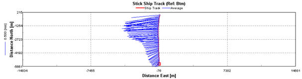 Fig.31. ADCP Ship Track and Average Flow Directions from Coastal to Offshore Transect |
|||||||||||||||||||
|
ADCP Conclusion For each profile shear could be approximated from analysing the change of velocity magnitude and direction between layers. In order to gain a full insight of the type of mixing at each station the ADCP data must be coupled with CTD data for the Richardson number to be calculated, which gives a numerical value for the type of mixing. Station 1: The fastest currents are found in the surface two metres of the profile, this is likely to be due a combination wind mixing and tidal mixing, due to station 1’s close proximity to the Falmouth Estuary. Backscatter intensity shows minima at the depths of 6m and 15m, with a slight increase in between these two levels, which could suggest the presence of zooplankton at this depth. The small directional fluctuation between depths could due to local topography, as it is only a small difference occurring throughout the column so is unlikely to be caused due to the tides. The average Richardson number at this station is 0.48, in between the two critical values, which for a coastal area is unexpectedly high, as one would expect a large amount of wind and tidal mixing. Station 2: Comparing the location of this station with that of the ADCP transect performed it appears that this data was collected very close to the position identified as the front. Therefore at this point one would expect the regime to be changing from well mixed to stratified. The average Richardson number at this point, 0.13, supports this as it is close to the critical value, so the water column is still mixed but close to the point at which stratification could occur. The backscatter profile shows a large amount of backscatter from the surface to a depth of 20m, but there is no clear increase that could represent a zooplankton maximum. Station 3: The lower layer of the faster flowing water found at station 3 flows 30° further to the North that the layer above, this is suggestive that there could be some shear between these two layers. The Richardson number is below the lower critical value, indicating the water is mixed, which is supported by the ADCP data. Station 4: The velocity magnitude and direction show little variation throughout the transect. These two factors suggest that there is little shear throughout the water column and that it could be a stratified body. This is supported with the comparatively high Richardson number of 2.49, which is above the critical values, suggesting the water column here is stratified. The backscatter profile again does not support the zooplankton data, as there is no dramatic increase in return signal seen in the surface layers. Station 5: The Richardson number at this station is 0.46, in between the two critical values, therefore at this station the mixing of the water column will depend on the previous conditions. This value suggests that station 5 could have been near the front where the water is in transition between mixed and stratified. There is also a thicker layer of backscatter at the beginning of the track, which could represent a bloom of zooplankton at this location; which would also support the idea that this station was sampled very near to the front. With the frequency of the ADCP set to 600KHz one would expect to see a significant increase in backscatter intensity at the zooplankton maxima. From our zooplankton sampling nets at each level the maxima was found to be at approximately 10m. Though at all stations there was no noticeable increase in backscatter intensity at this depth. This could be due to SPM have a more dominant influence over the level of backscatter, or the rough conditions creating bubbles creating noise which would disguise the signal from the zooplankton. The primary use of the ADCP instrument was to determine the amount of shear and mixing within the water column from coastal waters to offshore waters, with the intention of locating and describing the front, if present. The transect profile was very successful at this, as it gave a large response due to the dramatic decrease in velocity magnitude over the entire length. The station profiles gave a more discrete view and so it was harder to identify the mixing regime water in the surrounding area.
|
|||||||||||||||||||
|
Satellite Image With the use of MODIS sea surface temperature satellite images it’s possible to see the change in surface temperature in the surrounding coastline from Falmouth. An 8 day assembly was used, from the 11/06/2010 till 21/06/2010, in order to give more detail and to remove the effects of cloud cover, to allow a full picture of the coastline to be seen. The Lizard headland clearly causes a great deal of disturbance within the water column, as colder upwelled water can be seen surrounding this point. The effects of this can be seen more than 400km offshore. After which the temperature becomes warmer, which could represent the location of the boundary of the front, where the water has become more stable due to an input of buoyancy from surface heating.
|
Fig. 32. Satellite Image of Front NASA, 2010. Sea surface temperature, MODIS satellite. [online] Available: ftp://podaac.jpl.nasa.gov/pub/sea_surface_temperature/modis/data/terra/L3_mapped/sst/8day/04km/2010/. Accessed: 01/07/2010
|
||||||||||||||||||
|
Richardson number analysis Using data collected from the CTD and ADCP Richardson number was calculated for all 5 stations for 1metre depth increments. This provides information on the mechanical mixing within the estuary. Richardson number is basically the ratio of stratification to the square of shear in horizontal current. The critical values for the Richardson number are 0.25 and 1. Below 0.25 mixing is likely where as above 1 mixing is unlikely. Between the two a transition between the stable environment and mixing occurs. As the ADCP was on the underside of the vessel the closest values to the surface were at 2.35metres. There was also a difference between the CTD and ADCP depths so the CTD data selected as close as possible to the ADCP data.
Black rock is highly mixed and this is reflected by the Ri number with most depth falling well below 0.25 with only the depth 9.35 being above 1. This is due to its low velocity flow and differing flow direction between the two layers. The average at this station was 0.64 which is transitional.
Lizard point shows a mixed surface layer down to about 20 metres where mixing is unlikely. Although the average Richardson number is 0.2 which means on the whole this is a mixed location
Station 3 is a relatively mixed location as the average Richardson number is 0.17 although several values show transitional data as most values fall within the transition between mixing and stable. 0.17
The average at Station 4 is 2.43 which shows stratification although this average is skewed by the thermocline at a depth of 17 metres.
Station 5 shows a well mixed water column with stratification occurring at the sea bed. The average is 0.43 which represents a sporadic transitional location.
|
|||||||||||||||||||
|
Underway Sampling
Table shows the Temperature range during the Transect and the Bongo trawl, it also shows distance travelled. The major gradients in temperature are generally seen when moving from the shallower waters near the shore, to the deeper waters offshore. An exception to this was the region where we did the bongo trawl which had a sharp drop in temperature of around 1.5°C over a short distance in the direction of the shore.
|
Fig.33. Contour plot showing the underway sampling data for temperature, It highlights the temperature throughout the offshore sampling. The labels show the transect and bongo trawl, these were chosen based on the continuous samples highlighting areas where there was a large temperature gradient.
|
||||||||||||||||||
|
Light Attenuation The light attenuation data has been put into figures for each station, plotted with a trend line. The trend lines were used to determine the light attenuation coefficient for each station, further, the usable light depth was also determined for each data set. These values are found in table ...
The data collected at station 3 was considered unrealistic due to the shape of the graph when plotted, as the light decreased with depth to a point, then began to increase, which is why the results were considered erroneous. Station 4 is the station with the lowest light attenuation rate, and therefore the highest usable depth. Stations 1 and 2 are the most linear with a fairly constant attenuation rate throughout the column. Stations 4 and 5 are less linear, but still follow decrease at not too erratic rate. Station 3 is much more erratic, with the light increasing past a certain depth, as mentioned before.
Fig. 34. Station 1 Light Attenuation Plot
Fig. 35. Station 2 Light Attenuation Plot
Fig. 36. Station 3 Light Attenuation Plot
Fig. 37. Station 4 Light Attenuation Plot
Fig. 38. Station 5 Light Attenuation Plot
|
|||||||||||||||||||
| Offshore - Laboratory |
| Offshore - Laboratory |
|
Disclaimer This website and its contents do not represent the views of the University of Southampton or National Oceanography Centre including its staff and affiliates.
|
| Boatwork |
| Lab Work |
| Estuarine |
| Results | |
| Biological | |
|
Zooplankton In the estuary, zooplankton sampling took place at stations 1, 2 and 6. Station 1 and 6 were the same location, Black Rock, at the mouth of the estuary, but 1 was on the flood tide, and 6 was during slack water. Station 2 is found up river from station 1 and 6 at Turnaware point. The main zooplankton was copepods at all sites, with an estimation of 1057 per m³ at station 1, 336 per m³ at station 2 and 4933 per m³ at station 6. This shows a difference of 3876 per m³ between stations 1 and 6 at the different points on the tidal cycle. There is also significantly less plankton of any type at station 2 than the other two stations. Copepod nauplii were also present at on the slack water at black rock, in far smaller quantities on the flood tide and at even smaller quantities at station 2. The same goes for Cirripedia except none was found at station 2.
|
Fig. 87. Numbers and species of zooplankton found in net trawls
|
|
Phytoplankton Microscope transects showed a distinct lack of phytoplankton in the water samples, with very low numbers or organisms and a small range of species being observed.
|
|
| Chemical | |
|
Silicon The silicon vertical profile at stations 1 and 6 (Black Rock at different stages of the tidal cycle) showed a variable concentration with no apparent pattern, whilst stations 2 and 3 showed a decrease in silicon concentration with depth. Station 4 showed an increase in silicon concentration with increasing depth. The highest silicon concentration was 8μmol L-1 at station 2, 1m depth whilst the lowest silicon concentration was 2μmol L-1 at station 6, 25m depth.
|
Fig. 88. Vertical Profile of Silicon Concentration for Estuarine Stations
|
|
Silicon Mixing Diagram The silicon mixing diagram data points were clustered around salinity 33-35 but using the salinity 0 and 20 samples collected from the river near Truro, it was possible to see the mixing of silicon within the estuary. The mixing diagram showed a generally conservative structure with the data points plotting close to, although slightly below, the theoretical dilution line (TDL). There was a higher concentration of silicon at the riverine end member (110 μmol L-1) and a lower concentration of silicon at the marine end member (3 μmol L-1).
|
Fig. 89. Estuarine Mixing Diagram for Silicon
|
|
Phosphate The range in phosphate concentration over depth at all stations was low (0.0 – 0.4 μmol L-1) with much variation over depth and no clear pattern. The highest phosphate concentration was at 1m depth, station 2 (pontoon) with a concentration of 0.4 μmol L-1. The lowest phosphate concentration was 0.0 μmol L-1 at 13m stations 1 and 6 (Black Rock at different stages of the tidal cycle).
|
Fig. 90. Vertical Profile of Phosphate Concentration for Estuarine Stations
|
|
Phosphate Mixing Diagram The phosphate mixing diagram showed non conservative behaviour of phosphate as the points plot off the TDL at intermediate salinities (salinity of 20, phosphate 3.2 μmol L-1). The phosphate concentration was higher at the riverine end member (0.8 μmol L-1) than at the marine end member (0.0 μmol L-1) showing that the input of phosphate into the estuary was from riverine water (along with the other source at salinity 20).
|
Fig. 91. Estuarine Mixing Diagram for Phosphate
|
|
Nitrate Station 1 is located near Black Rock at the mouth of the Falmouth estuary. Nitrate concentrations remain relatively constant at 2µmolL-1 in surface waters down to 5m. Between 5 and 8m nitrate decreases by approximately 2µmolL-1, with a minima at 7.5m. Nitrate increases again by 1 µmolL-1 between 8 and 12m. Nitrate remains relatively constant between 12 and 25m. Station 2 was taken furthest upstream of Truro River. The Nitrate concentration peaks at 2m, though all three depths sampled give unusually high concentrations. Nitrate concentration increases by approximately 6µmolL-1 over the surface 2m. Between 2 and 5m nitrate concentration decreases rapidly by 10µmolL-1. Station 3 is located near the point where Truro River meets Saint Just Pool. Nitrate concentration remains relatively constant with depth at approximately 0.2µmolL-1. Station 4 and 6 had nitrate concentrations below the detection limit preventing detection of trends. Nitrate appears to be absent within the water column at these stations.
|
Fig. 92. Vertical Profile of Nitrate Concentration for Estuarine Stations
|
|
Nitrate Mixing Diagram The nitrate mixing diagram showed conservative behaviour of the nutrient with the data points plotting along the TDL. Nitrate concentration was highest at the riverine end member (400 μmol L-1) and lowest at the marine end member (0 μmol L-1) showing the source of nitrate within the estuary was riverine. The data points were concentrated at the higher salinities. |
Fig. 93. Estuarine Mixing Diagram for Nitrate
|
|
Oxygen Station 1 is located near Black Rock at the mouth of the Falmouth estuary. In the first 5m from the surface oxygen concentration increases and saturation deceases by approximately 4µmolL-1 and 0.5% respectively. This is followed by a sharp decrease in concentration and saturation over 2.5m by 15µmolL-1 and 6% respectively. This is followed by another sharp increase in oxygen concentration and saturation by 15µmolL-1 and 4% respectively over 4m. Finally there is a gradual decrease in oxygen concentration and saturation by 10µmolL-1 and 3% respectively. Station 2 is located towards the source of Truro River. Oxygen concentration and saturation increases rapidly in surface waters with depth by 25µmolL-1 and 10% respectively over 2m. Between 2 and 5m oxygen concentration only increases by approximately 3µmolL-1, while oxygen saturation decreases by 2%. Station 3 is located near the point where Truro River meets Saint Just Pool. Oxygen concentration and saturation shows a large decrease in the first 5m by approximately 25µmolL-1 and 10% respectively. This is followed by a sudden decrease of approximately 15µmolL-1 and 6% between 5 and 8m. Oxygen concentration then levels out at approximately 274µmolL-1 while oxygen saturation decreases by 2% over 4m. There is a final decrease in concentration and saturation towards the bed by approximately 10µmolL-1 and 5%. Station 4 is located the northern part of Saint Just Pool. Oxygen concentration shows little variance with depth remaining at approximately 274.5µmolL-1. Oxygen saturation shows a small decrease with depth from approximately 106% at the surface to 103% near the bed. Station 6 is located at Black Rock near Station 1. Station 6 shows a similar pattern in oxygen concentration and saturation to that of station 1. Oxygen concentration and saturation has become less stratified in surface waters than station 1, and is present in higher values. Oxygen concentration and saturation decrease by approximately 8µmolL-1 and 3% between the surface and 8m. Between 8m and 12m concentration and saturation increase by 18µmolL-1 and 6%, before decreasing again over the next 13m by approximately 34µmolL-1 and 14%.
|
Fig. 94. Vertical Profile of Oxygen Concentration for Estuarine Stations
|
|
Chlorophyll Station 1 showed no real changes in the top 12m of the water column, the highest reading of chlorophyll at this station was 0.8412µgL-1 (12m) after very slight increase (0.01 µgL-1) the concentration of chlorophyll declines steadily to the bed (25m) where it reaches a low of 0.357 µgL-1. Station 2 had a depth of 5m (the shallowest of the data set). The range of concentrations at this station was colossal from 0.9966 µgL-1 at 5m to 6.954 µgL-1 at the surface, this is most concentrated chlorophyll sample in the data set by 4.644 µgL-1 (next highest was at the surface of station 3, 2.31 µgL-1 ). Station 3 shows a great range of chlorophyll values from 2.31 µgL-1 to 0.4578 µgL-1, this occurs rapidly within a relatively shallow water column (when compared to the offshore where greatest decline was 0.9588 µgL-1, station 4). Station 4 shows a distinct chlorophyll maximum at 7m of 1.56 µgL-1, after this the concentration of chlorophyll declines gradually to 0.4518 µgL-1 (18m).Station 6 has a chlorophyll max at 12m of 0.7896 µgL-1; however the concentration at 8m does not fit the trend expected. Station 6 also has the smallest range of chlorophyll values in this data set, with the lowest concentration being 0.351 µgL-1 (at 25m).
|
Fig. 95. Vertical Profile of Chlorophyll Concentration for Estuarine Stations
|
|
Discussion For the chlorophyll results Station 1 was taken at Blackrock, which is at the boundary between offshore and estuarine waters, here the waters were well mixed and so there is very little difference in chlorophyll. Station 2 was taken at the shallowest part of the estuary that we could get to, we were tied up to a pontoon where there were other boats moored up. The extreme chlorophyll values when looked at with the nitrate values from the lab (fig …) show nitrate concentrations of 2.5952µM (5m), 11.46 µM (2m) and 6.5098µM (1m). This correlates with the high chlorophyll concentrations and thus confirms that the water column is eutrophic at this station. The reason that the nitrate is higher slightly below the chlorophyll max is because the phytoplankton will be in greater numbers at the surface and then as they die they will sink lower and decay releasing nitrate. Station 3 was the second shallowest station with a max depth of 16m; this could explain why there was such a large range as the water column is concentrated. It was also far up the estuary near station 2 where the water was eutrophic. Station 4 shows the expected trends and reveals that they is a zooplankton community living below the chlorophyll maximum , thus explaining the rapid decline below the maximum at 7m. Station 6 was a repeat of the station at Blackrock, but at this time the tidal state was different - slack tide. During this station the boat drifted quite a bit and this could explain the anomalous result at 8m. The absence of pattern in silicon distribution over depth could result from silicon concentrations being consistently low as a result of phytoplankton utilisation of silicon in the spring bloom. Stations 2 and 3 were further up the estuary, with a higher silicon concentration in the surface. As silicon concentrations are generally higher in freshwater sources, this could indicate a layer of fresher water at the surface of the estuary, possibly with higher silicon concentration as a result of run off from surrounding silicate rocks. The low concentration of silicon at 25m depth for station 6 (Black Rock: the most marine station) could reflect the very slow remineralisation process of siliceous phytoplankton frustules left from the spring bloom. That the data plotted slightly below the TDL might indicate a removal process for silicon within the estuary. This could result from utilisation of silicon by siliceous phytoplankton, such as diatoms, or a flux to the sediment. The nitrate concentration plotted slightly below the TDL, suggesting possible removal of nitrate at higher salinities. This could be due to the utilisation of nitrate by marine phytoplankton or as a flux to the sediment. The higher phosphate concentration at station 2 can be explained to a certain extent by the mixing diagram, as phosphate is supplied by the river and so one would expect the highest phosphate concentrations to be at the lower salinities: station 2 was the furthest station sampled up river and had the lowest salinities. The low phosphate concentrations at 13m depth at station 1 and 6 (Black Rock) could be due to phytoplankton utilisation at an intermediate depth approaching the thermocline. That the data did not plot along the TDL indicates non-conservative behaviour of phosphate within the estuary. The higher phosphate concentrations at salinity 20 could result from an additional source, such as agricultural run off, flux from salt marshes, flux from sediment, an additional riverine source or even sewage treatment works. At Station 1 nitrate has been used by the previous phytoplankton bloom at approximately 7.5m. Below this depth nitrate increases as the phytoplankton is restricted to surface waters. At Station 2 there is low tidal mixing causing less saline estuarine waters to be restricted to the surface while highly saline waters are restricted to the bed, creating a salt wedge. Therefore high nitrate levels produced by terrigenous inputs are trapped at the surface. At stations 3, 4 and 6 nitrate has been consumed by previous phytoplankton blooms, leaving low concentrations throughout the water column. At Station 1 and 6 oxygen has been produced by the previous phytoplankton bloom at approximately 5m. Below this depth oxygen is consumed by the increased abundance of zooplankton. At Station 2 there is a peak in oxygen associated with a peak in nitrogen, facilitating phytoplankton growth. At Station 3 there is low tidal mixing with less saline estuarine waters confined to the surface bringing high nutrient content allowing for accelerated phytoplankton growth and high oxygen levels in surface waters. At the peak of Oxygen at 20m is associated with an increased level of phytoplankton activity, due to the presence of a. At depths below this zooplankton levels are increased producing higher levels of respiration than photosynthesis, and so oxygen is consumed.
|
|
|
CTD Station 1 was located near Black Rock in the mouth of the Falmouth Estuary. Station 1 shows a temperature decrease of approximately 2oC within surface waters. A thermocline occurs at roughly 13m, where temperature levels out. Transmittance increases with depth, leveling out at approximately 13m, coinciding with the thermocline. Salinity remains fairly constant with depth at 35.1, indicating a well mixed water column. Station 2 was located towards the source of Truro River. We find a temperature decrease of approximately 2oC over 6m, with a thermocline occurring at 2m. Temperature remains fairly constant in surface waters, decreasing after 2m. Transmittance remains fairly constant with depth until 2m where it begins to increase with depth by approximately 0.16V over 4m. Salinity is low in surface waters and relatively higher in bottom waters, with a halocline forming at 2m. This suggests less dense estuarine river water with a salinity of approximately 32.9 is running over denser sea water with salinities as high as 34.4. Station 3 is located further along the estuary at the point where Truro River meets Saint Just Pool, near Turnaware Point. There is a small almost linear decrease in temperature with depth of approximately 2oC. Transmittance is constant at approximately 4.19V until 4m, where it begins to increase with depth until 8m by approximately 0.6V. Transmittance decreases slightly at the seabed. Salinity increases with depth by 0.8 suggesting a poorly mixed water column with fresher less dense water overlying denser sea water. Station 4 is located in the northern part of Saint Just Pool. There is a decrease in temperature of approximately 2oC over 18m. A thermocline is seen at 5m with constant surface temperatures of 15.6oC. Between 5 and 10m temperature decreases sharply by approximately 2oC, leveling out after 10m. Transmittance is constant in surface waters until 5m where it increases from 4.28 to 4.35V by 10m coinciding with the thermocline, before decreasing again by 0.3V. Salinity increases in the first 3m before leveling out at approximately 15.3. This suggests station 4 has better vertical mixing then station 3, but still has a small volume of fresher less dense water overlying denser sea water. Station 6 is located at Black Rock near Station 1. Temperature has become stratified with a thermocline forming at approximately 12m. At the thermocline temperature decreases sharply by 0.8oC. Temperature decrease more steadily after 13m by 0.4oC. Transmittance remains fairly constant with depth at a relatively high level of 4.39V. Salinity remains fairly constant with depth suggesting a well mixed water column with relatively high salinities of 35.1.
|
Fig. 54 - Station 1 CTD Data Plot
Fig. 55 - Station 2 CTD Data Plot
Fig. 56 - Station 3 CTD Data Plot
Fig. 57 - Station 4 CTD Data Plot
Fig. 58 - Station 6 CTD Data Plot
|
|||||||||||||||
| ADCP | ||||||||||||||||
|
Transect One The first transect was carried out using an ADCP across the mouth of the estuary from Black Rock, between St Anthony’s Head and Pendennis Point. A minor change in velocity of the water body was evident when crossing the mouth of the estuary, reaching a peak velocity around 0.5m/s at the eastern end. The direction plot showed turbulent mixing in the first few hundred meters, settling into a southerly current. Backscatter plots from the first transect indicated limited particulate matter in the water column, yet there were some pockets of slight disruption within the first few meters of the waters surface. The true wind speed ranged from 5.2 knots at the start, to 9.3 knots at the end. The stick ship track plot showed the water direction to be uniform throughout.
|
Fig. 59. Estuarine Transect 1 ADCP Velocity Magnitude
Fig. 60. Estuarine Transect 1 ADCP Velocity Direction
Fig. 61. Estuarine Transect 1 ADCP Average Backscatter
Fig. 62. Estuarine Transect 1 ADCP Ship Track
|
|||||||||||||||
|
Transect Two Velocity was variable with no defined peaks across the transect, the average water speed was about 0.2m/s. The direction plot showed Northward water movement and some in easterly and westerly directions also. There is large scale variation in backscatter within the small area sampled, with shallow pockets of backscatter at the surface reaching down only a few meters. Overall backscatter was approximately 60dB.Wind speed was 7.2 knots.
|
Fig. 63. Estuarine Transect 2 ADCP Velocity Magnitude
Fig. 64. Estuarine Transect 2 ADCP Velocity Direction
Fig. 65. Estuarine Transect 2 ADCP Average Backscatter
Fig. 66. Estuarine Transect 2 ADCP Ship Track
|
|||||||||||||||
|
Transect Three The ADCP profile of Turnerwave point, taken at 12:10 GMT, showed a consistent magnitude of between 0.00m/s and 0.25m/s. Some areas, notably those close to the surface in the shallow zone, displayed increased velocity. The direction flow of the water was not uniform across the transect and gave no clear direction of movement. Backscatter levels were higher near the surface of the shallower areas, with a defined change around 5 meters. The stick ship track showed a change in water direction around the Bill Conway at the start of the transect. Wind speed was 9.9 knots.
|
Fig. 67. Estuarine Transect 3 ADCP Velocity Magnitude
Fig. 68. Estuarine Transect 3 ADCP Velocity Direction
Fig. 69. Estuarine Transect 3 ADCP Average Backscatter
Fig. 70. Estuarine Transect 3 ADCP Ship Track
|
|||||||||||||||
|
Transect Four The forth transect was just north of Messack Point, taken at 12.59 GMT. The Velocity/magnitude data did not show a high flow rate, though there was a clear flow direction. The water in the top 15 meters was moving to the North West, while the water body beneath moved in a southerly direction indicating stratification. Small amounts of stronger backscatter were visible only in the surface meter. Otherwise there was a uniform low level of back scatter through out. The Stick ship Track revealed variation of average water direction of the boat. Wind speed 12.8 Knots.
|
Fig. 71. Estuarine Transect 4 ADCP Velocity Magnitude
Fig. 72. Estuarine Transect 4 ADCP Velocity Direction
Fig. 73. Estuarine Transect 4 ADCP Average Backscatter
Fig. 74. Estuarine Transect 4 ADCP Ship Track
|
|||||||||||||||
|
Transect Five The fifth transect, taken across the estuary just south of the Messack Creek, recorded a very weak velocity of the water column, but there was a distinct difference in direction of the water. The surface 5 meters moved southward. The channel though had turbulent flow below 5 meters to the sediment surface. Increased levels of backscatter at the surface were seen and the averaged wind speed for this location was 12 knots. The current was strongest in the west of the estuary, with flow to the south.
|
Fig. 75. Estuarine Transect 5 ADCP Velocity Magnitude
Fig. 76. Estuarine Transect 5 ADCP Velocity Direction
Fig. 77. Estuarine Transect 5 ADCP Average Backscatter
Fig. 78. Estuarine Transect 5 ADCP Ship Track
|
|||||||||||||||
|
Transect Six Black Rock was sampled for the second time in the day. This time water speed was very weak and the shallows also had some faster movement close to the surface. The wind speed had increased to 12 knots. The flow direction was south, out of the estuary and turbulence was present close to the bottom of the channel. The surface layers show signs of increased backscatter, but lower down the water column was a more uniform level of backscatter. The Stick Ship Track indicated that the average current was unidirectional and the west side of the estuary had a much stronger current with an overall southerly flow.
|
Fig. 79. Estuarine Transect 6 ADCP Velocity Magnitude
Fig. 80. Estuarine Transect 6 ADCP Velocity Direction
Fig. 81. Estuarine Transect 6 ADCP Average Backscatter
Fig. 82. Estuarine Transect 6 ADCP Ship Track
|
|||||||||||||||
|
ADCP Discussion Stations one and six show the same location at two times of the day. The first was recorded at 08:50 GMT and then again at 14.19 GMT. High water was at 08:52 at Falmouth, with an extra 6 minutes added on for the distance to Truro. The difference in velocity of the water is due to the difference between Flood tide and Slack tide from the two tracks respectively. Stick Ship Lines confirm a change in current direction of 1800 taking place during slack water. There was a change in backscatter in the water column between the transects, which correlated with an increase in wind speed, from 5.2 knots to 12 knots. This appeared to be the main reason for the increase in backscatter on the second transect of Black Rock, as there was limited chlorophyll, or zooplankton variation. Station two was the furthest up the estuary that we sampled. There, water velocity was mixed due to the tidal cycle, because the readings were taken at slack water. (If the estuary had been ebbing or flooding the movement would have been faster). At slack water the conflicting direction causes a slower movement of water, along with a large variation in the direction of the water, as was recorded. When the ADCP data for this station was compared against that of chlorophyll data, there is a clear indication of the cause of the amount of backscatter in such a shallow area. The chlorophyll readings for this station were in the high, between50 and 60, far above the estuaries average. This fitted with the ADCP profile. At Station 3 slack water caused the direction of the flow to be inconsistent, yet have uniform, though weak, flow speed; this is typical slack tide data. Unlike station 2 the ship stick plot is not in northerly flow direction, but more southerly as it followed high tide. The chlorophyll data is consistent with limited backscatter. At station 4, north of Messack Creek there was a strong body of water that was moving in a southerly direction, with overlying waters moving in a north westerly direction. It is interesting to see that only a few hundred meters south at station five there was a dramatic shift in flow direction to southerly water in the upper 10 meters of the channel and the bottom few meters are more turbulent. This is most likely due to the input of water from the creek; it is also the reason for the change to a unidirectional flow of the ship stick in the profile during station 5. The average backscatter is fairly similar. Due to sample number limitation it is hard to compare the two points with regard to backscatter, as no phytoplankton was collected.
|
||||||||||||||||
|
Estuary Underway Sampling Start Time – 08.16.15 BST End Time – 15.08.44 Start Latitude - 50° 09.469 Start Longitude - 5 03.244 End Latitude - 50° 08.988 End Longitude - 5° 02.053 Underway sampling was conducted on the estuary for the entirety of the day, where T/S probes were used to take measure of any change in temperature or salinity throughout the day sampling the estuary, from water taken at the surface continuously using a pump. The measurements were taken when any large change in salinity occurred. The salinity of the water was constantly monitored, and any large changes were recorded, this method of monitoring was used as opposed to samples at certain times as time samples could miss large changes of salinity. When processing data, the data collected at 10.03, 10.04, 10.09 and 10.10 had to be considered erroneous as the samples were contaminated by bubbles in the water, giving readings that were too low, and considered anomalies. Fig... shows the salinity as a contour plot, with lines showing constant salinity, the stations where CTD vertical profiles, and ADCP transects were take.
|
Fig. 83. The Full salinity range falls between 32.7 and 35.3 for all of the estuary samples. The diagram shows that as the latitude (or distance from oceans influence) increases the salinity decreases, with the highest salinities falling around black rock where the freshwater influence is far less (stations 1 and 6).
|
|||||||||||||||
|
Estuary Richardson number analysis The Richardson number for the estuary data was calculated using both the ADCP data and CTD. As the CTD didn’t provide a density, a computer program was used to calculate it. The program required temperature, salinity and depth to provide the density at the depth. Richardson number was calculated for Black Rock at 08:49 and 14:45 GMT and Woodbury Pontoon this allows for a range of stations along the estuary as well as a time comparison.
As all the Richardson values are below 0.25 this represents mechanical mixing taking place. As this across the whole water column it coincides with the flooding tide mixing the water at the time the data was taken. At this station the average Ri number was 0.028 which shows a well mixed estuary.
Woodbury Pontoon was a shallow station and so it is difficult to discern too much from the data. This was the furthest point sampled within the estuary. As the Richardson numbers between 2 and 4 metres are above 0.25 metres this represents a transition. The average for this point was 0.43 and so this is a transition point. This is due to the sporadic nature of the slack tide that was effecting this point
The Richardson numbers for the second Black Rock station show similar values except at 17 metres depth where the value is 1.4 this represents that mixing is unlikely at this depth. This represents the transition into the deepest part of the channel. The average Ri number for this station was 0.092 showing a well mixed area. |
||||||||||||||||
|
Light Data
The k values calculated with the use of the irradiance meter and secchi disc correlate very strongly, even though the secchi disc values are all more than twice as large as the light irradiance meter values. Station 1, the most marine station, recorded at black rock, has the lowest K value of all the stations, for both the secchi calculated value and irradiance meter calculated values. The k value is a numerical description of how well light will penetrate through the water column; it is influenced by the rate of absorption by matter within the water column. A low value of k, such as the one seen at this station, represents a water column in which light will penetrate a large distance, due to a lower level of absorption. Station 2, the most riverine station, has the highest value for K of all the stations, again for both the secchi and irradiance meter calculated values; the light here will therefore only penetrate a short distance, as the level of absorption will be high. Station 3 and 4’s k values are close in comparison and both lie between the upper estuary value and the estuary mouth values The light irradiance data from station 5 was not plotted, as during taking these recordings the underwater meter drifted under the boat. Therefore these data cannot be used in comparison to the other stations.
|
||||||||||||||||
|
Light Data Discussion The irradiance meter is likely to give much more accurate results in comparison to the more “rough and ready” secchi disc. There was a high level of correlation between the k values of these two methods, but little agreement. This is likely to be due to the perception of the person responsible for taking the secchi depths, which were all uniformly larger than expected. At the mouth of the estuary, station 1, the k value was at its lowest, donating that light is able to penetrate deepest, as the levels of absorption are lower. This could be due to low abundance of phytoplankton and suspended material, the latter we cannot prove, but the former, the abundance of phytoplankton, can be seen from our phytoplankton nets taken at each station. The overall levels of phytoplankton were very low …….., suggesting that the presence of suspended matter had a larger influence on the value of k at each station. Station 2 was taken furthest up the river and gave the highest value of k, therefore light could not penetrate as deep at this location. As previously discussed the abundance of phytoplankton is unlikely to be the cause of this, instead the previous nights heavy rain is likely to have had a larger influence. By comparing the k value here, with the results from the ADCP transect, one can see high levels of backscatter, which could represent a large amount of sediment having been churned up and carried by the now stronger flow of the river. The values from stations 3 and 4 lie in between those of 1 and 2, as expected, as the amount of suspended material would decrease with dilution and settling along the course of the river. Had the transmissometer been functional during the practical one could have compared the results from this with the k value, which would have given a further description of the optical properties of the water column.
|
||||||||||||||||
|
Fig. 53. Google Earth Estuary Location Map
|
Methods for estuaries On the 7th of July 2010, the vessel RV Bill Conway was used to survey the Fal estuary. Samples were taken at 5 stations along the estuary and various physical, chemical and biological measurements were obtained. During this practical, several measurements were taken at each station. A CTD and rosette frame were used to gather information on temperature, salinity, fluorometry and light. Attached to the rosette were five 2.5L Niskin bottles, which were used to take water samples at different depths in the water column. An Acoustic Doppler Current Profiler was also used to measure direction and velocity of currents within the water column. Plankton nets were deployed at some stations, and these nets were 200microns mesh size, and 50cm diameter. Measurements of light, and depth of the euphotic zone were obtained by use of a secchi disk, and a light meter. This light meter consisted of a surface downwelling light probe, which remained out of the water, and a underwater downwelling probe which was lowered into the surface water. Underway temperature and salinity measurements were also taken using an onboard pump, and a temperature/salinity probe. Station 1 was located at the mouth of the Fal estuary, at Black Rock. A horizontal transect was taken across the estuary, and measurements were obtained, using the hull mounted Acoustic Doppler Current Profiler. After completing the horizontal transect, vertical samples were taken in the deepest part of the channel. This was done through the use of the CTD, and it provided information on the nature of the water column. Once this data was received, a decision was made on how many samples would be taken and at which depths. Samples were taken using Niskin bottles. At this station, all 5 bottles were used to take samples, to ensure all the equipment was in working order. Measurements of light, using both the light meter and the secchi disc were carried out at this station, along with the deployment of a plankton net. Station 2 was located at Woodbury Point, at the source of the estuary. A horizontal transect was also taken at this station, and ADCP measurements were taken. Three water samples were taken at this station, at depths of 5m, 2m and the surface, as the depth of the water column only reached 7.4m. As before, light measurements were taken, and plankton net was deployed. Station 3 was located at Turnerwave point, further down the estuary, towards the mouth. A similar method of experimentation was used at this station also, with water samples being taken at five different depths. These depths were chosen in relation to the thermocline. A sample was taken at the bottom of the water column, below and above the thermocline, within the thermocline, and at the surface. A horizontal transect across this part of the estuary was also taken, and ADCP data was recorded. Identical to previous stations, a horizontal plankton sample was done, and light attenuation was measured. Station 4 was located at a wider point, further down the estuary, at North Messack point. The experimental methods used at this station, were very similar to those of the stations before. However no plankton net was deployed as storage capacity had been supposed. Station 5 was located further seaward than that of Station 4. Once again, no plankton net was deployed. Water samples were taken at five different depths. These depths were chosen in relation to the thermocline, along with one at the surface, and maximum depth. Station 6 was located, once again, at Black Rock in order to collect comparable data to that of Station 1. This enabled an attempt to compare the variations in physical and chemical properties at different stages in the tidal cycle. The methods of data collection at this station were the same as station one, with the exception of the plankton sample. In addition to these set stations, underway monitoring of salinity was also taken. This was achieved using a Temperature/ Salinity probe. This probe was placed in a bucket on board, which was continually filled by a pumping system. Changes of 0.5 salinity units were recorded, and any significant changes were sampled and sent to the lab for analysis. This was done to help investigate the changes in the chemical properties within a tidal cycle.
|
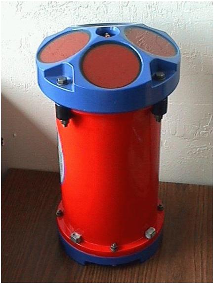
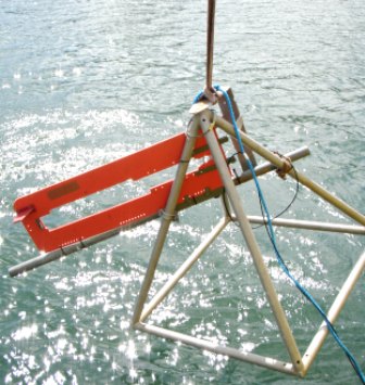
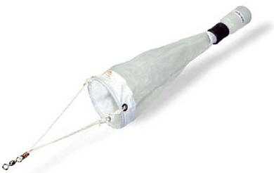
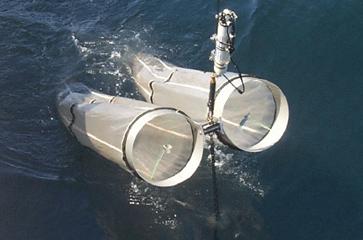
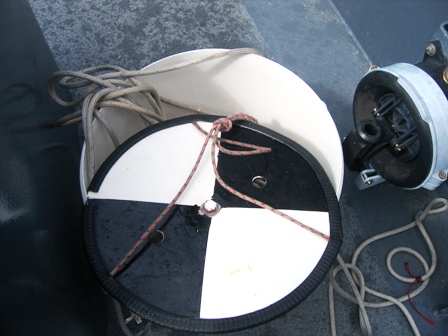
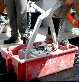
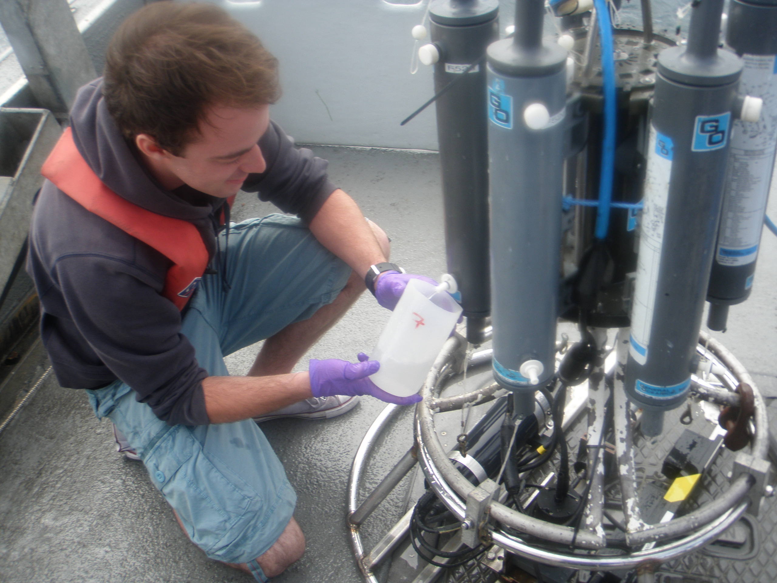
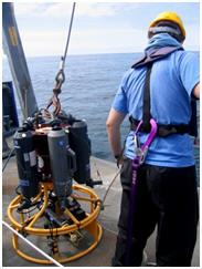
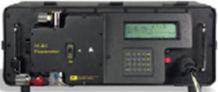
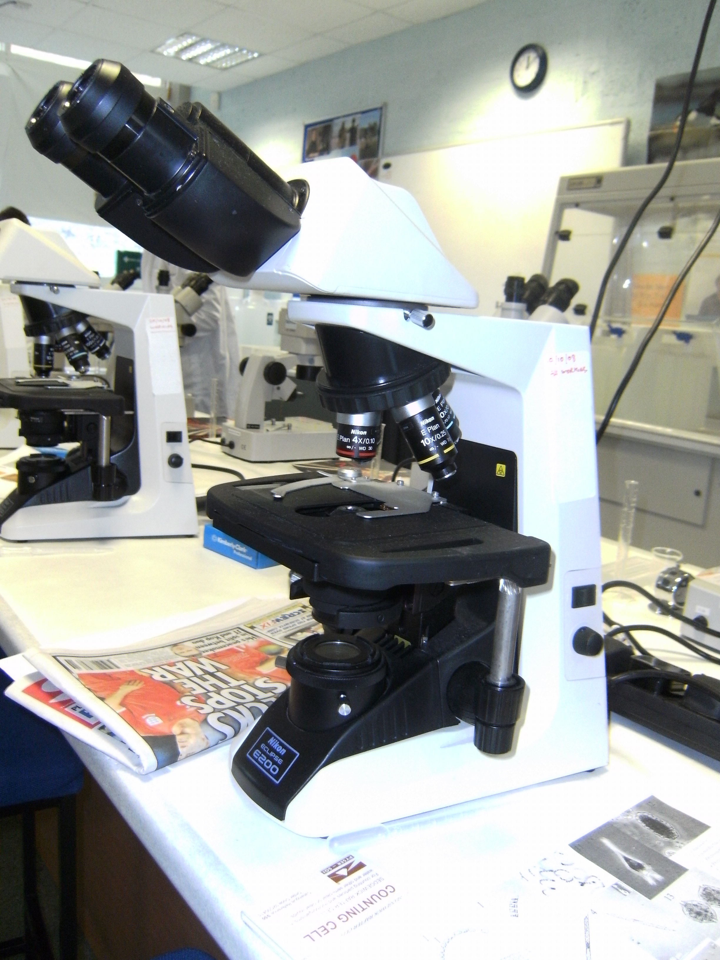
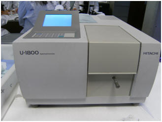
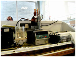
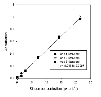
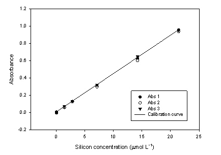
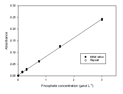
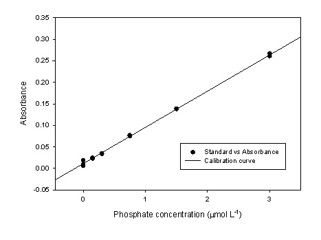
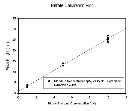
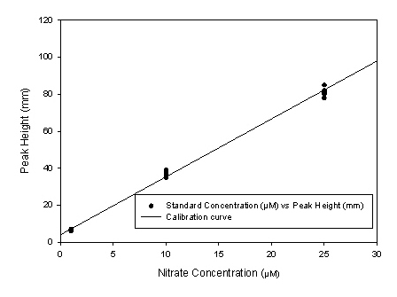
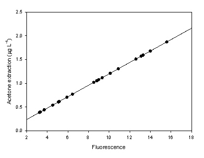

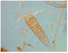
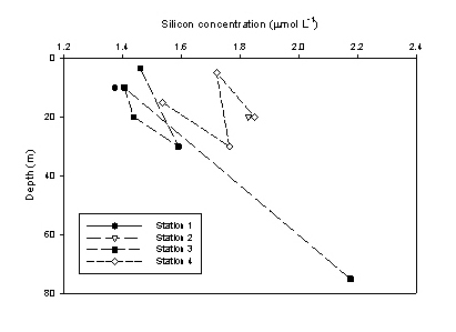
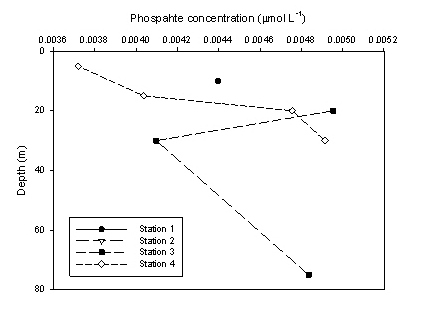
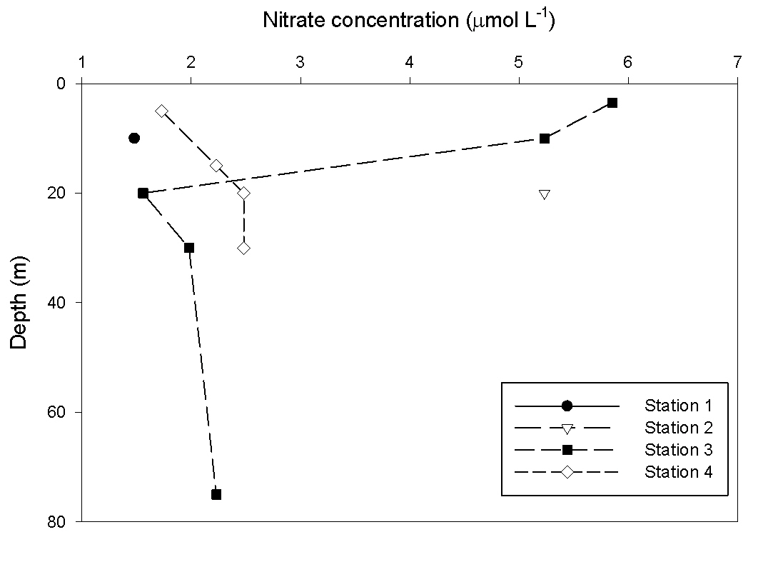
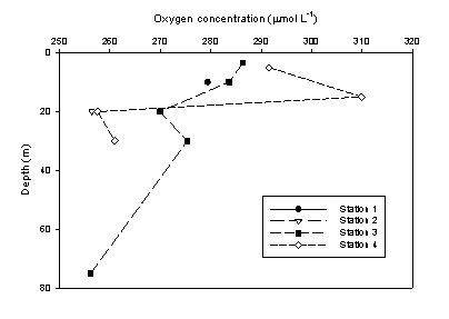
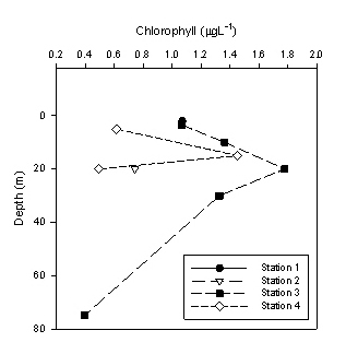
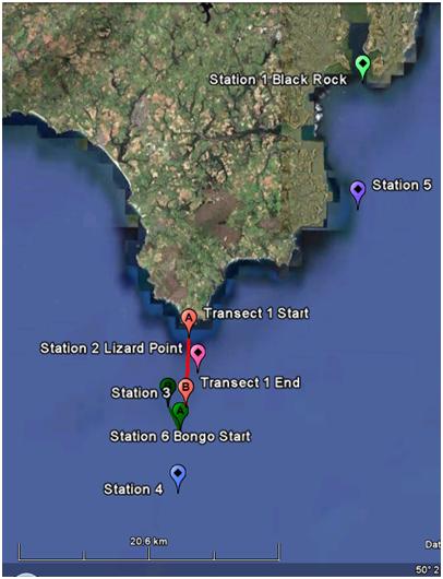
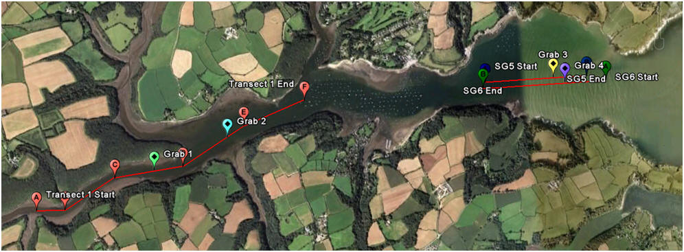
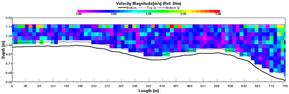
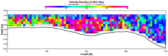
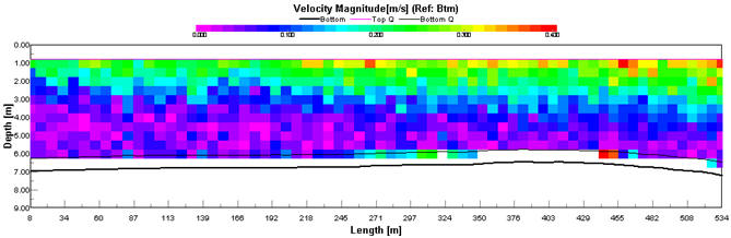
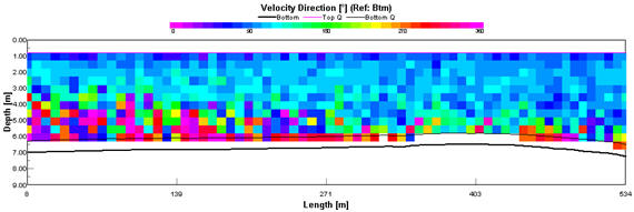
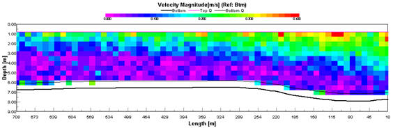
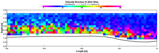
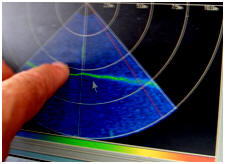
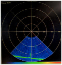
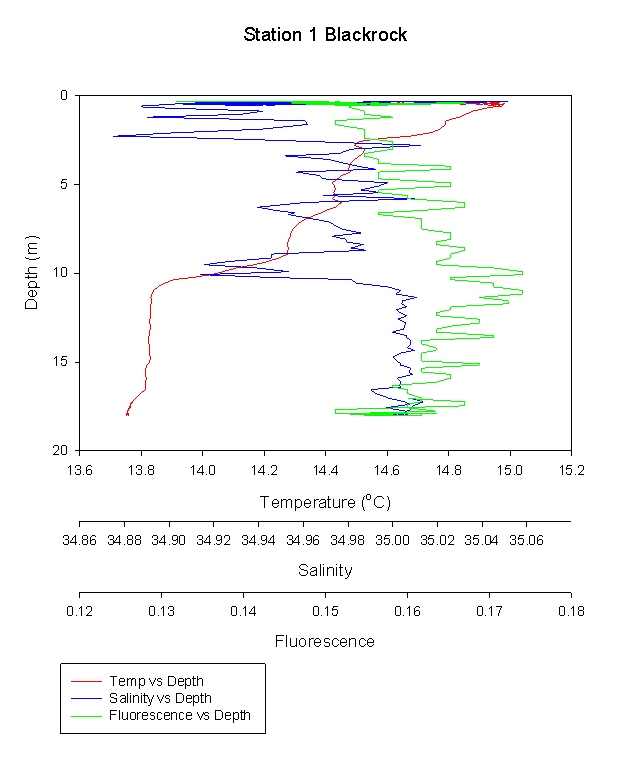
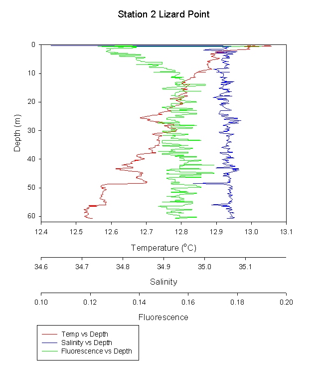
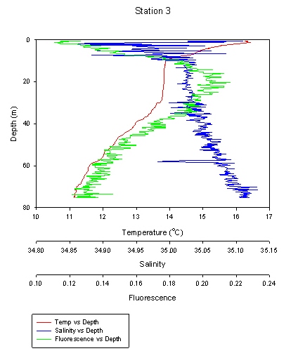
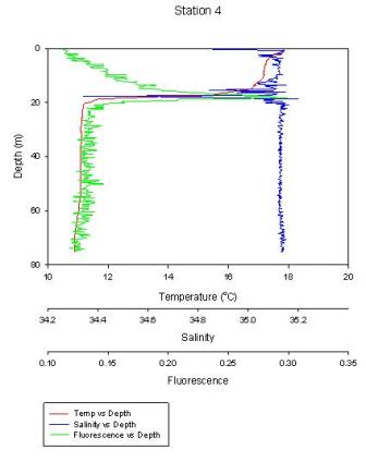
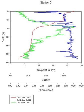
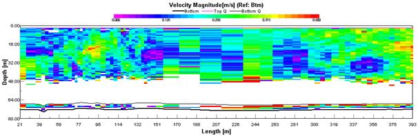
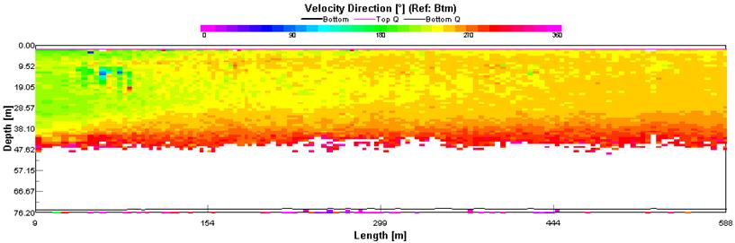
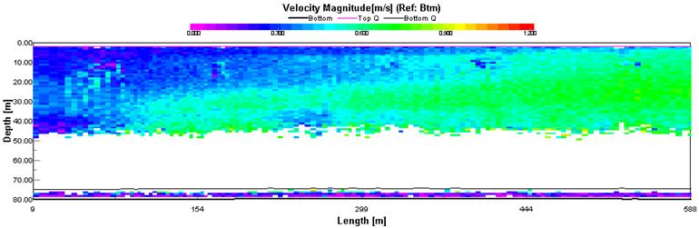
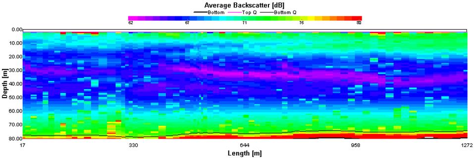
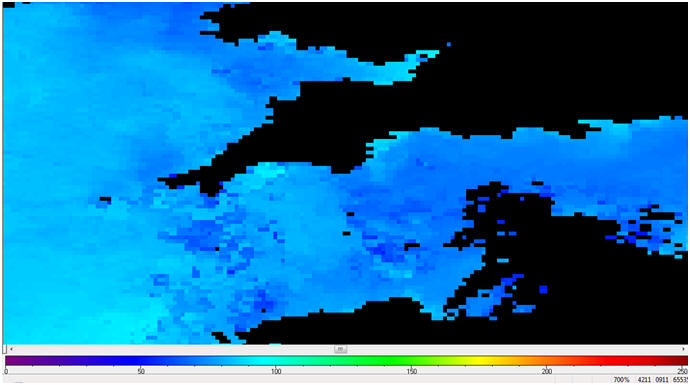
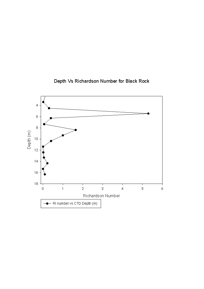
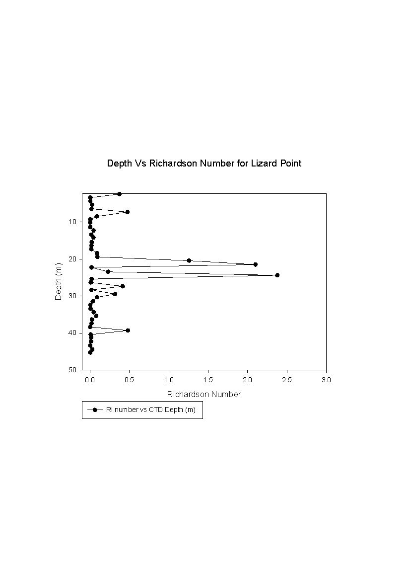
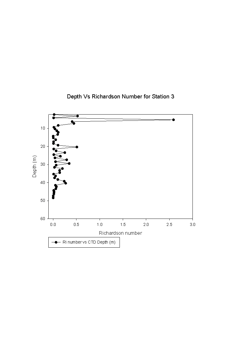
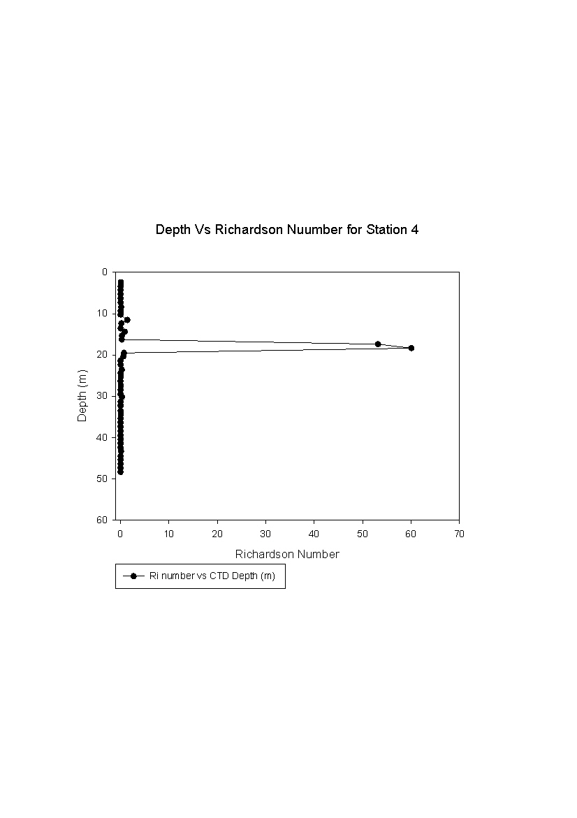
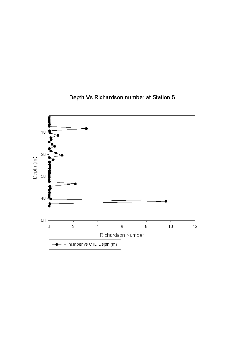


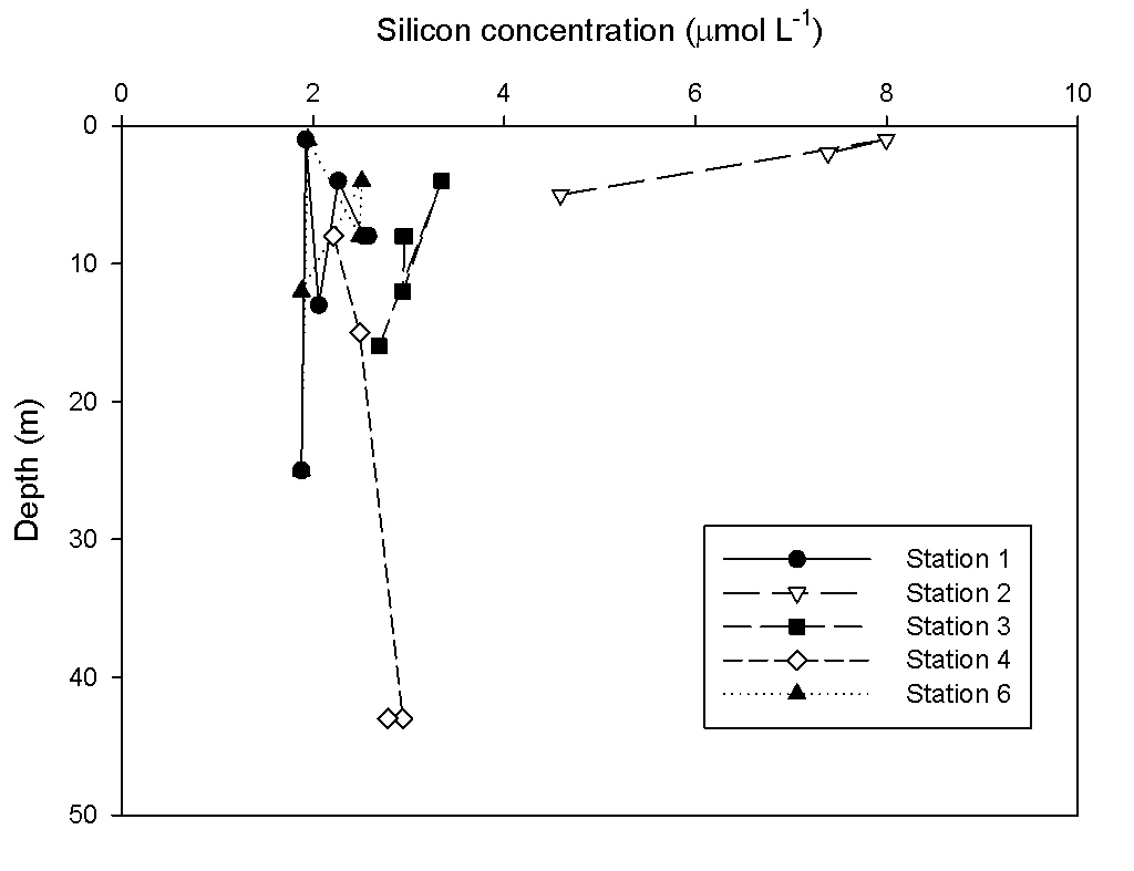
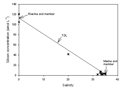
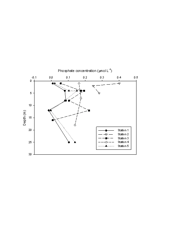
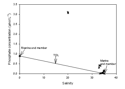
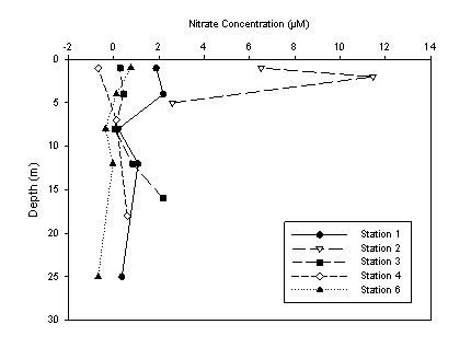
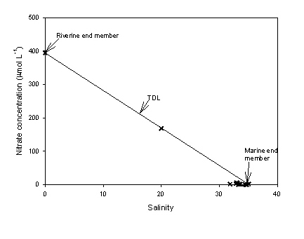
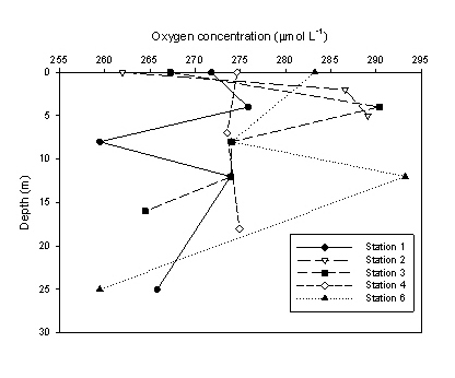
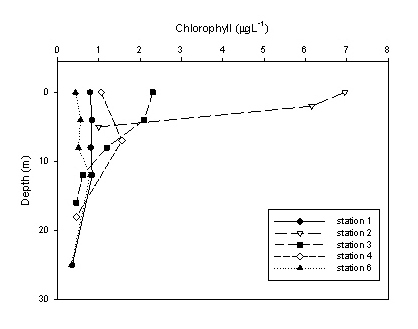


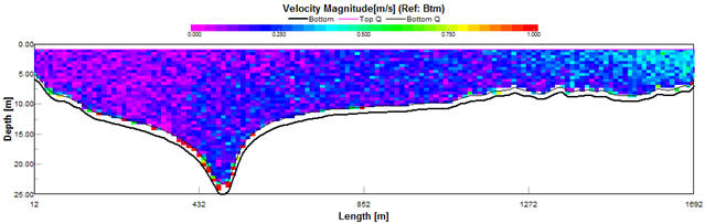
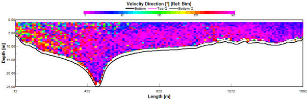
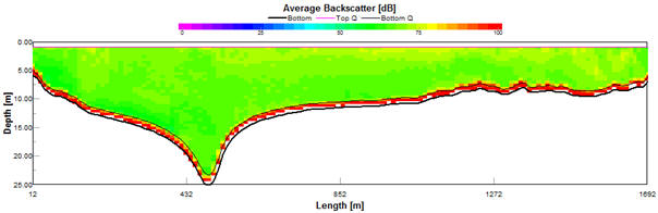
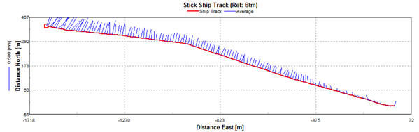
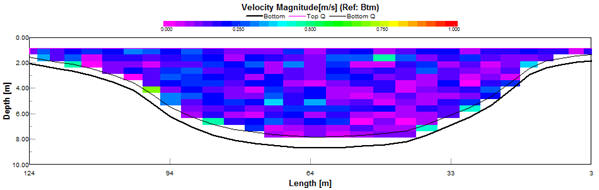
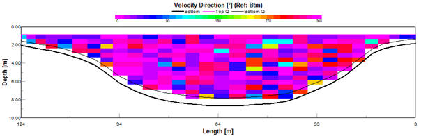
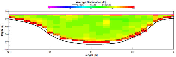
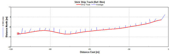
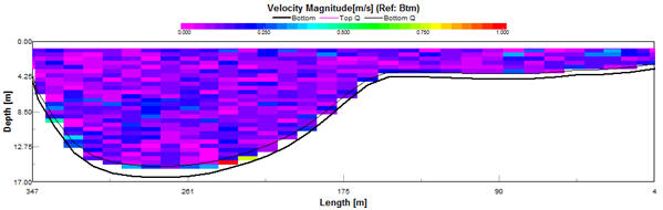
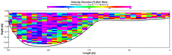
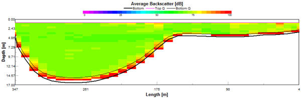
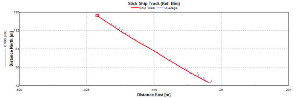
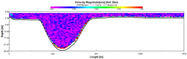
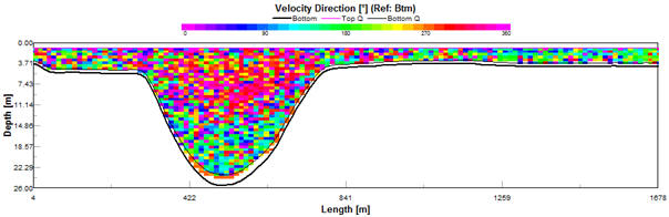
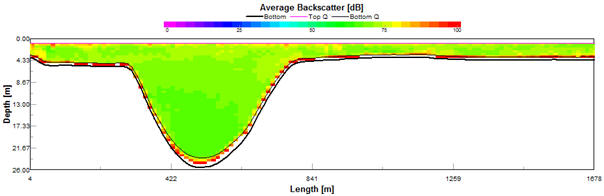
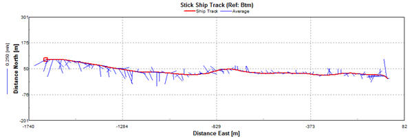
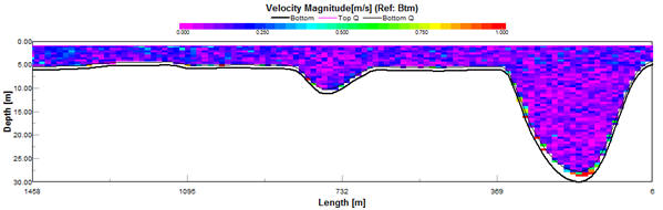
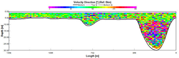
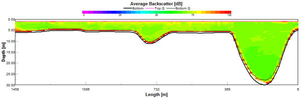
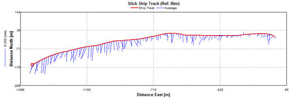
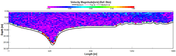
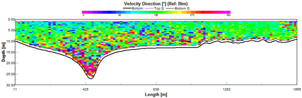
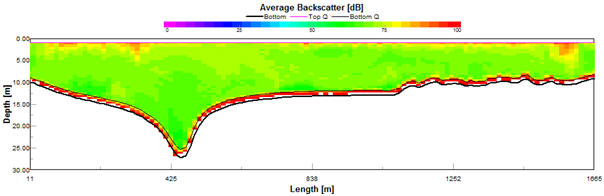
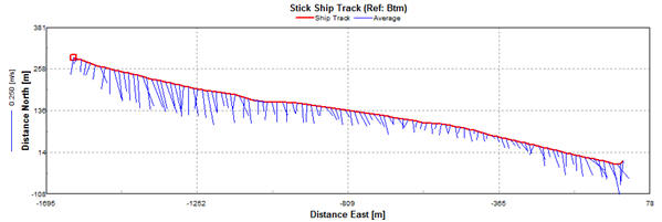

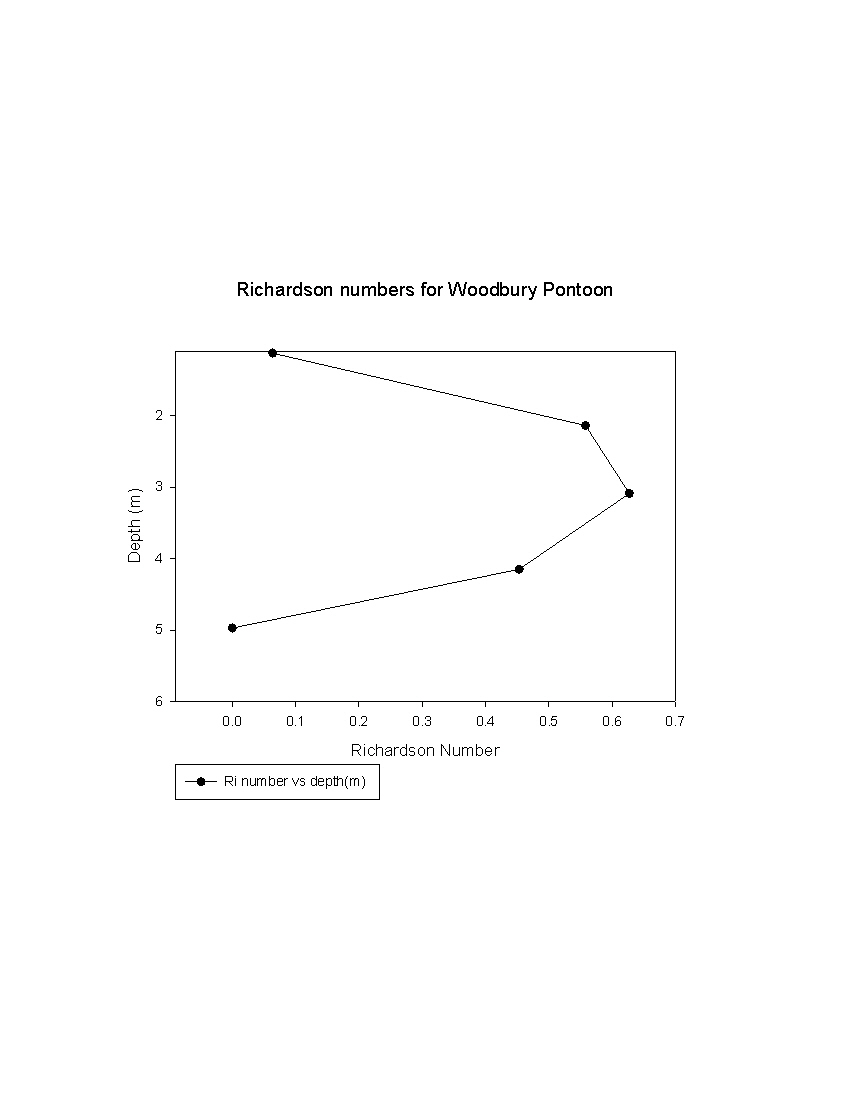
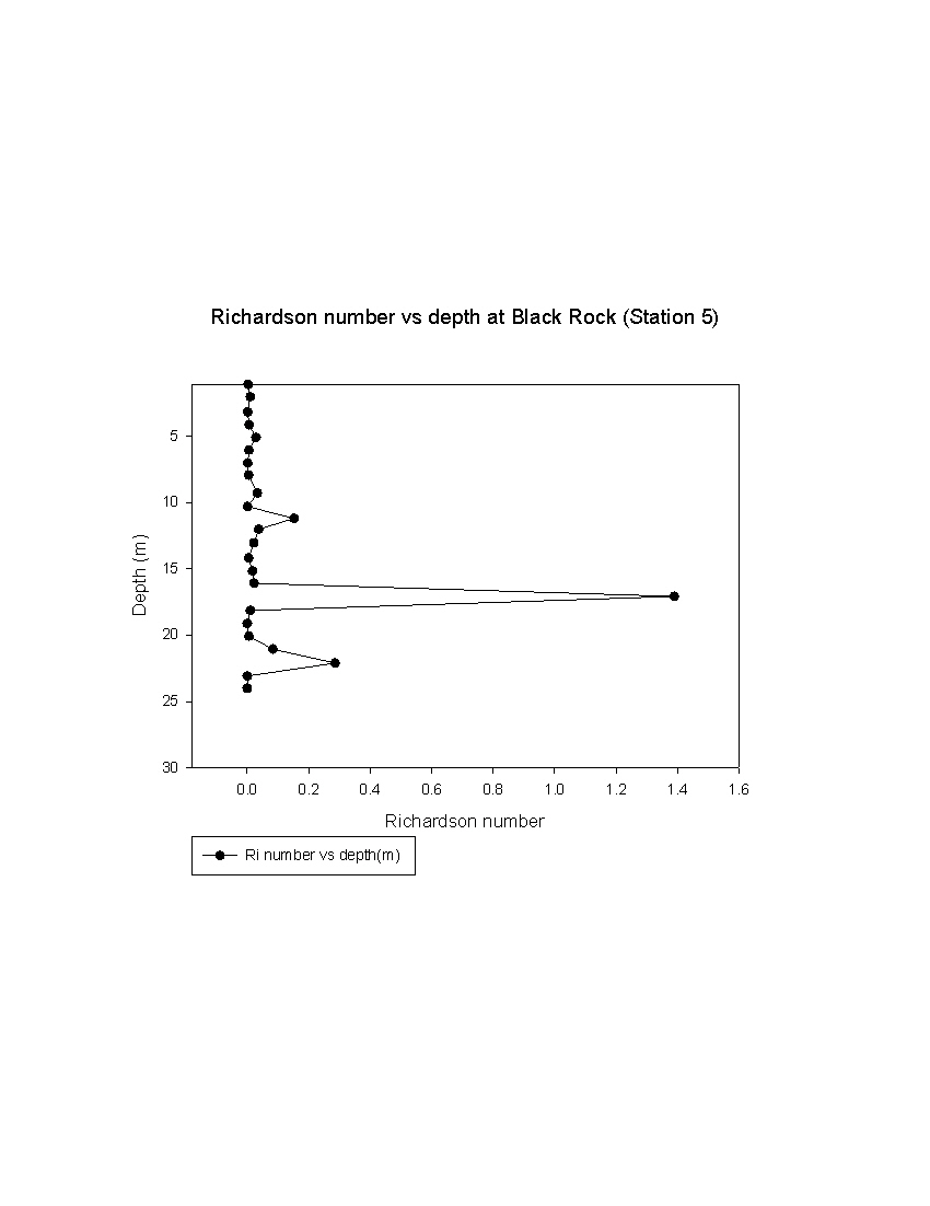
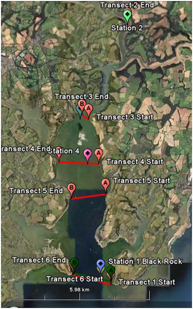