
An Oceanographic investigation into the Fal estuary and offshore area

Edmund Burgon
Harry Davies
Lawrence Eagling
Ben Edwards
Catherine Hollyhead
George Holmyard
Julian Johnson
Joshua Pedder
Diana Shores
Kate Spillman
Joanna Wooles
|
|
An Oceanographic investigation into the Fal estuary and offshore area |
|
| Edmund Burgon Harry Davies Lawrence Eagling Ben Edwards Catherine Hollyhead George Holmyard
|
|
Julian Johnson Joshua Pedder Diana Shores Kate Spillman Joanna Wooles |
|
|
|
|
|
|
|
|
| Introduction | |
|
The Fal estuary is located in South West Cornwall, England. The key source is the Truro river which is joined by five other main rivers (The Tresillian, Pill creek, Restronguet creek, Mylor creek and Penryn river) and as many as twenty eight smaller tributaries to make it one of the largest natural harbours in the world (following such harbours as Sydney and Poole). The Fal is a ria (drowned river valley) that formed due to sea level rise many thousands of years ago and is now the deepest estuary to be found within the UK. The shipping channel starting in the outer tidal basin, known as Carrick roads, can reach up to 34m in depth. The estuary can be described as a macrotidal environment with spring tides having a range of approximately 5m with the range decreasing to a more mesotidal scale further up the estuary (Pirrie et. al, 1997). Due to a large tidal range, a tidal current of approximately 2 knots and low freshwater input the Fal estuary can be described as well mixed. Though the amount of industry present directly in Falmouth has decreased dramatically over the last few decades it is still susceptible to anthropogenic influences that may severely affect the quality of the water and therefore the Fal as a stable environment. The Falmouth dock area and surrounding marinas cause sewage, oil and contaminants to be released into the surrounding water, also due to large amounts of farming in the surrounding countryside the estuary is subject to agricultural run off. Many problems could possibly arise from this, for example eutrophication which has been thought to have caused the first toxic red tides of Alexandrium tamarense in 1995, and the linking of TBT in antifouling paints has been proven in many studies to cause infertility in species of gastropods in the Fal (Gibbs, 2009). Another problem in the Falmouth and Helford area is the large amount of metal pollution that is causing ongoing problems for the estuary; the Fal has been described as the most metal polluted estuary in the UK (Bryan and Langston, 1992). This is due to the surrounding area having been heavily mined since the Bronze Age, in particular when the mining industry peaked in the 19th century, millions of tons of tailings were remobilised from the Carnon valley and ended up being deposited in the Restronguet creek (Langston et. al., 2003). The last active mine (Wheal Jane) was finally closed in 1991 though residual drainage from these abandoned mines still add to pollution in the Fal today. An area of 6387.8 ha, including the Falmouth and Helford has been designated as a Special Area of Conservation (SAC no. UK0013112). The Fal is of particular interest due to its varied substrate being home to many diverse communities. For example the sublittoral sandbanks support seagrass species such as Zostera noltii and Zostera marina, also present are the UK’s largest Maerl beds (such species as Phymatolithon calcareum and Lithothamnion corallioides) which in turn harbour many epifaunal and infaunal species including rare species such as Couch’s Goby (Gobius couchi) (JNCC website). Another reason for its classification as SAC is the presence of Shore Dock (Rumex rupestris) throughout the area. (JNCC website) |
|
|
|
|
|
|
|
|
|
| Boat Information | ||
| Description | Specification | |
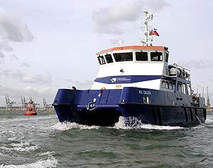
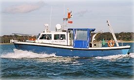
| RV Callista
|
RV Callista is a 20m twin hull
purpose built research vessel with a large rear deck and ‘A’ frame for
equipment deployment. Has a hull mounted ADCP with 600KHz, CTD and
Rosette, flourimeter, transmissometer, on board pump and Dry and Wet
lab.
|
• Length- 19.75m • Breadth – 7.40m • Draft – 1.80m • Depth Midship – 2.85m • Max speed - 50 knots • 4 tonne ‘A’ frame • 1.5 tonne Capstan • 2 x side Davits @100kg each • Range – 400 Nautical Miles • Max persons: 30 + 4 crew
|
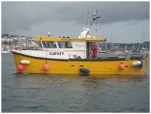
| Bill Conway
|
Scientific research vessel used for survey work, teaching, research and diving. Equipment onboard includes CTD and Rosette, ADCP, secchi disk and light meter.
|
• Length- 11.74m • Breadth – 3.96m • Draft – 1.30m • Depth Midship – 2.85m • Max speed - 10 knots • 750kg ‘A’ frame • 0.25 tonne Capstan • 2 x side Davits @50kg each • Range – 150 Nautical Miles • Max persons: 12 + 2 crew |
| RV Xplorer
|
Xplorer can survey both inshore and offshore and is equipped to deploy midsized equipment from the working open stern deck for bathymetric surveying. On board there is a Van Veen Grab, underwater camera and Towfish (side scan sonar).
|
• Length- 12.00m • Breadth – 5.20m • Draft – 1.20m • Max speed - 25 knots • Helia deck Crane with winch • Tonne Capstan • 2 x side Davits @50kg each • Max. Persons: 12 + 2 crew
|
|
|
|
|
|
|
|
|
| Equipment information | |||
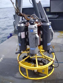 |
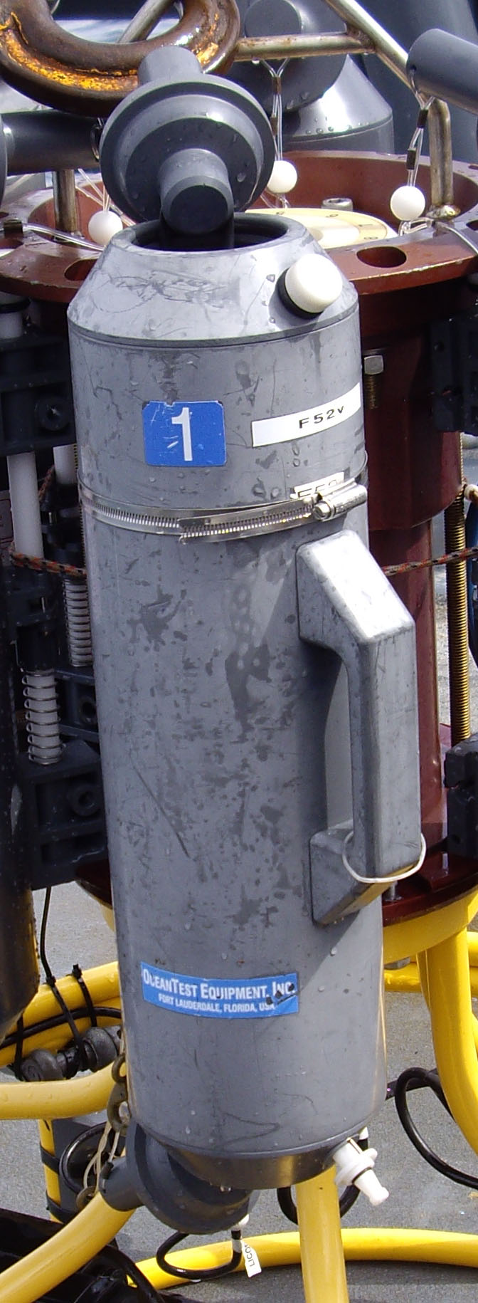
CTD (conductivity temperature depth) profiler is used to measure temperature, salinity and depth measurements and to provide information on the vertical structure of the water column. Continuous measurements are made as the CTD is deployed approximately every cm of depth and monitored onboard in order to determine sampling depths. The salinity is measured via the conductivity of the water, the temperature by a thermometer and depth with a pressure sensor. The CTD is attached to a rosette system for collecting water samples along with other instruments. The difference in height between the centre of the CTD bottles and measuring instruments is approximately 0.5m. |
|
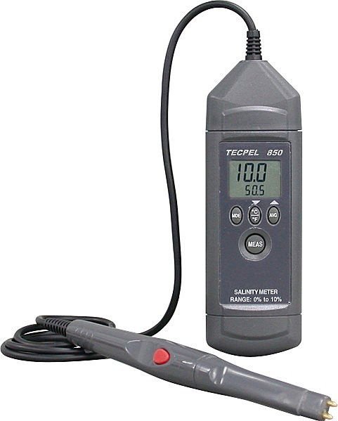
T/S probe The T/S probe measures temperature and salinity of the water. The salinty is measured using the conductivity of the water from a current passing between two metal plates. The temperature is measured via a thermistor which decreases its resistance with increasing temperature.
|
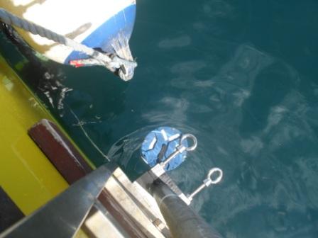 |
ADCP ADCP is used to measure current flow velocities along transects. By measuring the Doppler shift of a given parcel of water, using three sound beams in different planes, the flow direction and flow velocity can be calculated. The ADCP can also be used to detect backscatter, indicating areas of high Zooplankton/Phytoplankton (large species of) abundance. |
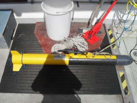 |
Sidescan sonar Sidescan sonar (towfish) is used to map the seabed to identify sediment types, possible habitats and areas of interest for grab samples. The images are produced in black and white onto paper and displayed on a computer screen. Darker lines represent areas of higher reflectance eg. harder or rough sediment types, and identify elevated or lowered bed forms. |
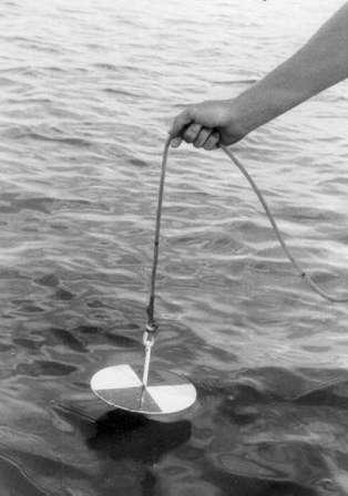 |
Secchi disk A Secchi disk was used to estimate the depth of the euphotic zone, the disk is divided into 4 quarters 2 white and two black and is lowered into the water column until no longer visible. The depth from the surface to the disk is measured and multiplied by 3 to an approximate for the euphotic zone. The secchi disk depth in metres is converted to attenuation coefficient where k = 1.44/secchi depth. |
 |
Niskin bottles The Niskin bottles were used to collect water samples at given depths for oxygen, chlorophyll and nutrient analysis. Each bottle has a 5 litre capacity (on board Callista), and can be individually closed at depth via the onboard computer. Bottles are attached to a Rosette system on the CTD profiler, with a total of 5 bottles being able to be fired at any depth along the profile. |
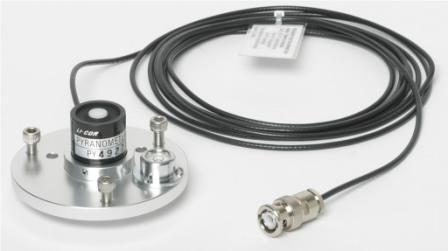 |
Light meter Works via a lambertian surface cosine collector made from opal and measures the downwelling light in the water column, the light is absorbed and the photons are then converted to an electrical signal. |
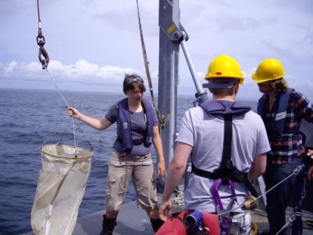 |
Plankton Nets These nets are either towed behind or lowered off the boat. For zooplankton, a 200µm mesh was used with a 500mm diameter mouth. A bongo net was also used during towing, in order to gain both zooplankton and phytoplankton samples. These are used in combination with a flow meter in order to gain a quantitative figure of how much water has passed through the filter, and as such the concentrations of plankton within that area of ocean. |
 |
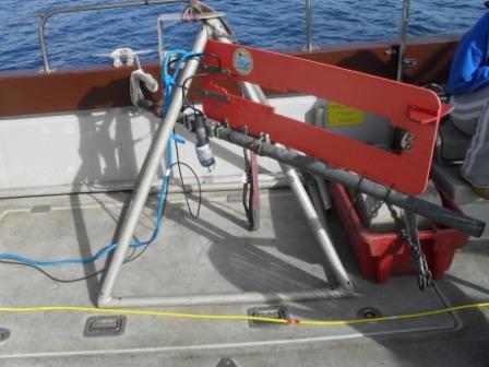
Van Veen Grab A Van Veen grab is a galvanised steel long arm grab sampler which is triggered to close on impact with the seabed. The Grab has a sample size of around 0.01m3 and is used to collect soft sediment for identification normally graded through sieves. |
|
Transmissometer Transmissometer, which is attached to the CTD, is used to determine the attenuation of light in water by measuring the SPM (suspended particulate material). It works via a transducer emitting pulses into the water column and then measuring the energy return, thus working out the SPM. |
|
|
Fluorometer A fluorometer is used to measure fluorescence in the water to infer chlorophyll concentrations throughout the water column. This instrument works by emitting a pulse at a specific wavelength (around 380nm) into the water, as the water becomes light saturated it emits a corresponding pulse of around 675nm which is picked up by a detector attached to the CTD rosette. |
 |
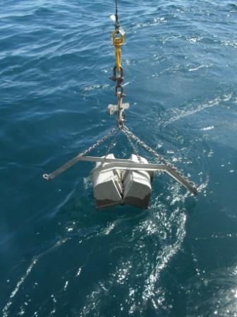
Video camera Video mapping captured by a video camera mounted on a scaffolding frame is lowered to the sea bed and images are projected on a screen and recorded. These images are used to identify habitat and sediment types and benthic fauna for identification purposes and to ensure no need for blind grab sampling.
|
|
|
|
|
|
|
|
|
| Estuarine | ||||||||||||||||||||||||||||
|
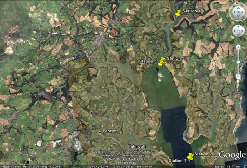
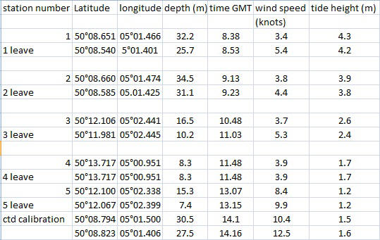
Introduction: Aims: On the 29/06/2010 an investigation into the physical, chemical and biological parameters of the Fal estuary was carried out (Table1.). Aboard the Bill Conway, a variety of instruments and procedures were used to try to gain an understanding of the temporal and spatial variations of these parameters within the estuary, also to see how the estuary acts a transition zone between freshwater input and coastal waters. To ensure sampling against the tide the boat was first directed to Black Rock at the seaward end of the estuary where vertical profiles were recorded using CTD equipment. Other CTD profiles were also taken at designated locations throughout the estuary. While underway and heading towards the riverine end of the estuary, parameters were also measured horizontally. ADCP data was collected for multiple transects spanning the width of the estuary. Objectives: · Use CTD and ADCP to collect and observe vertical profiles of salinity, temperature, light attenuation and current structure. · Use CTD to measure the nutrient, chlorophyll and plankton distributions. · Use T/S probe and onboard pumping system to collect samples for nutrient chlorophyll and plankton distribution and assess conservative and non conservative behaviour of the nutrients. Equipment used: CTD rosette, Niskin Bottles, T-S probe, Secchi disk, light meter, plankton net, ADCP.
PSO: Diana Shores. |
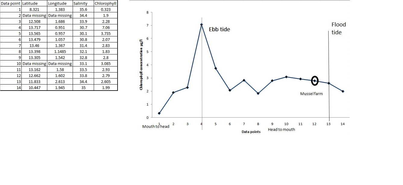
Table1. Location and parameter values for estuarine stations.
|
|||||||||||||||||||||||||||
|
Physical: Method: Five transects were taken throughout the day using an Acoustic Doppler Current Profiler (ADCP-600 KHz) viewed via an onboard laptop using WinRiver software. Profiles in the different areas show flow velocity, direction and the particulate matter from the backscatter. Four of the five transects were measured in conjunction with CTD profiles. The transects up the estuary were taken across Turnaware Point and the pontoon, on the return journey transects were taken at the King Harry ferry, Turnaware point (to observe any changes) and at Black Rock. Two methods were used to measure the light penetration depth, a Secchi disk deployed in conjunction with a CTD and a light meter. The disk was lowered into the water column until it was no longer visible to the eye. The distance from the surface to the Secchi disk was measured and recorded. A light probe was also used to measure light penetration depth. A probe measured light at the surface whilst a second probe is lowered into the water to predetermined depths. Meter markers on the rope allowed a crude depth measurements to be taken. Measurements were recorded in µmol/m2/s1. A CTD attached to a rosette system with Niskin bottles allowed CTD profiles and sampling to be undertaken simultaneously. After preparation of the Niskin bottles the equipment was deployed via an A frame and winch. A CTD profile was recorded and observed during the surface to depth journey. Using this information, sample bottles were closed via the onboard system on the return to the surface. Data collected was directly entered into a laptop during the sampling using Microsoft excel. Recorded times in the data set are in GMT. |
||||||||||||||||||||||||||||
|
Fig5. Velocity magnitude plot for Station 3
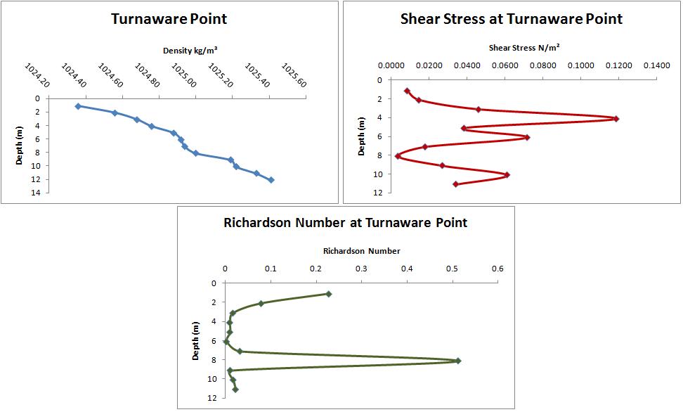
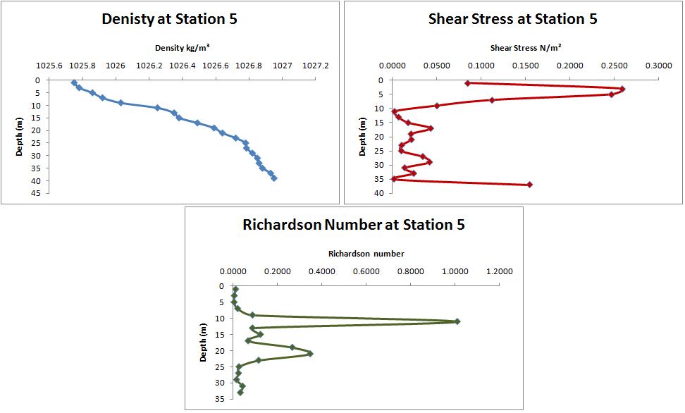
Fig6. Change in density, shear stress and Richardson number with depth at Turnaware point (station5)
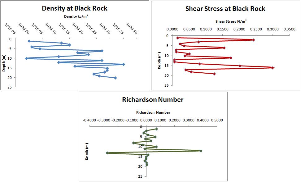
Fig7. Change in density, shear stress and Richardson number with depth at Blackrock point (station1)
|
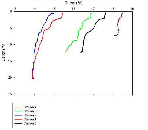
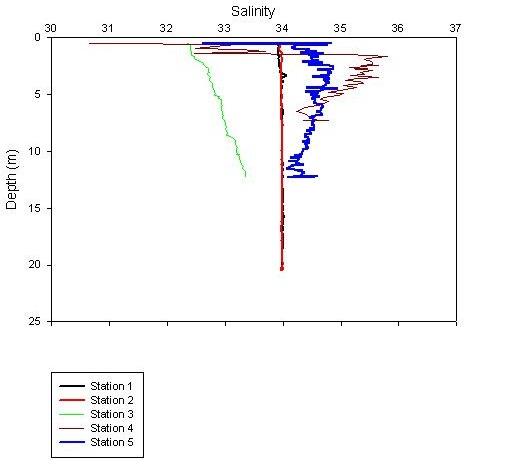
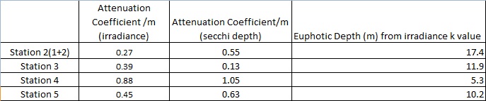
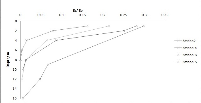
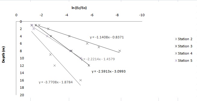
Analysis: Vertical profiles from the CTD of surface temperature across the five stations ranges from 15.4°C at station 2 (the most seaward station) to 19.1°C at station 4, and, at depth between 13.9°C at station 2 to 18.6°C at station 4, which has the shallowest recorded data set of the five stations and is the most riverine member of the stations sampled (Fig.1). Vertical profiles of temperature and salinity at the two most seaward stations (1 and 2) showed the water column to be very well mixed with regards to salinity. The two stations show relative homogeneity with depth for temperature (Fig.1), with slight stratification occurring within the surface 5m and becoming well mixed further down the water column. Shallow haloclines are present in the top 3m at stations 4 and 5. Station 4 showed the highest surface temperature (19.1°C) and lowest surface salinity (30.7) which is to be expected as it was sampled furthest from the estuary mouth. From the salinity profiles (Fig.2) it is apparent that the Fal estuary has a low freshwater input as the riverine samples did not show large decreases in salinity; any freshwater is observed on the surface of the water column due to it being of a lower density. From the vertical temperature profiles the water column throughout the estuary contains areas of mixed and stratified water with more mixing processes occurring towards the seaward end. This would suggest that the estuary is more partially mixed than well mixed at this time of year and that the mixing processes are relatively tidal dependent. ADCP at Station 3 (Fig5.) (CTD Station) shows on the velocity magnitude plot that from the seabed to around 6m depth there is shear acting on the current reducing velocity (0.125 – 0.250ms-1), between 6m depth to surface the shear is reduced causing the velocity to increase to a range between 0.250ms-1 – 0.375ms-1. The velocity direction plot depicts a two layer structure with the slower shear affected layer moving in a northerly direction and the upper layer moving in a southerly direction due to the ebbing tidal flow. The ships track data show the gradual change of direction in the flow from 7m. At 11.6m depth the reverse flow is total. The total depth of the water column in the centre of this transect is 15m. Station 4 (CTD Station) is a relatively homogenous velocity magnitude plot, direction is southerly throughout the water column coinciding with the ebbing tide. Down flow of the mussel farm a transect was carried out without a CTD profile. The results of the ships track showed some change in water column direction at 8.5m depth, by 11m depth there is a strong flow in the opposite direction to the ebbing tide. This transect was taken 1 hour prior to Low Water time in Falmouth. Station 5 (CTD station) shows an increase in velocity in two areas, one at the top and another at the bottom of the water column. The ship’s track shows a relatively large number of eddies throughout the water column profile. The two layered water column structure is still visible with decreased flow rates. Track taken 30minutes before Low water time in Falmouth. Station 6 (CTD Station) unidirectional flow with the tide. The charts available do not have diamonds on to ascertain low water times closer to the spatial sampling points. ADCP data suggests a two layered water column develops towards the head of the estuary with the surface layer flowing with the prevailing tidal current and the bottom shear layer acting as a flood tide. This acts as a time lag, delaying low water time higher up the estuary. Turnaware Point (Stations 3 and 5) (Fig6.) is at the mid part of the estuary and flow is gentle. There is a gentle density gradient with a range of 1.05 kg/m³ and no strong pynocline is present. The Richardson number results show a layer of moderately stratified water at 8m depth and the shear stress can be seen above and below this layer of stratified water as friction between the layers causes turbulence. Above and below 8m the water is very well mixed. Black rock is at the mouth of the estuary and water is very fast flowing and turbulent (Fig7.). The density with depth shows that this is a very unstable water column subjected to a very high level of mixing. Shear stress is high at most depths due to the many different layers of water at different densities flowing in different directions. The results of the Richardson numbers are very erratic and show many layers of very stratified water and many layers of very well mixed water. These results however may not be accurate as the measurements are taken at large depth intervals. The light attenuation coefficient increases (Table2. and Fig3 and 4.) from the seaward end member (Station 1, k=0.27m-1) to the most riverine end member (station 4, k=0.88m-1), indicating an increase in particulate matter with distance from the mouth of the estuary. Salinity values taken in the estuary reveal little freshwater input from riverine flow therefore it is probable that the higher attenuation coefficient is due to re-suspension of sediments as the estuarine depth shallows. In general, k values <0.5 are required for phytoplankton blooms (Iriarte and Purdie, 2004) indicating insufficient light with depth at station 4 to generate a phytoplankton bloom yet sufficient at the other stations for a bloom to be generate. However, the results show the highest phytoplankton concentrations at station 4 (0.29ml-1) and a relatively low concentration at the other stations (0.1ml-1) suggesting that light is not the limiting factor for this temporal estuarine data set. The zooplankton results indicate that station 5 has had a major bloom, it is probable that the grazing in this area is in part responsible for the low phytoplankton count. Using a secchi disk to determine light depth is a less accurate way of measuring than using the sensor. The measurement is subjective as dependant on the individual so for consistency it is best to have the same person estimate the depth at each station. This was done during this exercise. The residence time (Tres) is defined as the time it takes to replace the total volume of freshwater within the estuary with “replacement” water from the rivers. It therefore provides an indication of how long pollutants introduced into the estuary will remain before being flushed out to open ocean. One mathematical method of calculation is based on the ratio of total volume of freshwater (Vfreshwater) to the river flow rate (R). To calculate the Vfreshwater the freshwater fraction (f) is obtained from the following formula: (s=salinity)
Values for the Fal river flow rates are available from hydrographic station operated by the Environmental Agency at www.nwl.ac.uk/ih/nrfa/webdata (station number 048003). The month of June shows an average input of 1.082m-3s-1 over the years 1978 to 2007 with peaks of 2.878m-3s-1 in January. However there are numerous other tributaries into the estuary and current data is unavailable. The V total can be estimated from length dimensions on charts and using mid tidal range values. CTD data taken on the survey can then be used to calculated the mean salinity and obtain the sea salinity value. Based on the uncertainties of the data available a residence time has been estimated by using previous group’s calculations and taking the lower value based on the fact that the previous weeks in June were very dry and so the riverflows were reduced. Residence time is estimated at 60 days. |
Fig1. Vertical profile of temperature vs depth for the five stations sampled with a CTD.
Fig2. Vertical profile of salinity vs depth for the five stations sampled with a CTD. Table2. attenuation coefficients calculated two ways, one using slopes of the station as per Fig4, the second using secchi disk measurements recorded at the stations. One percent light depth has been calculated using the slope coefficient.
Fig3. attenuation of light in the Fal estuary for the stations sampled, shows and exponential diminution of downward irradiance.
Fig4 . using the ln log of fig3 has enabled the slopes to be calculated to calculate the attenuation coefficients for the stations.
|
||||||||||||||||||||||||||
|
Chemical: Method: Initially horizontal water samples were to be taken every 2 salinity change. The salinity change was determined by using a TS probe placed in a bucket which had water pumped into it from 1m depth. On the return journey from near the head to the mouth samples were taken every 0.5 salinity change. The more frequent sample collection from head to mouth was due to salinity not significantly changing up the estuary and ample sample bottles were available. The samples were filtered into two sets of sample bottles (plastic bottles for silicon concentrations and dark glass bottles for phosphate and nitrate concentrations) by forcing 60ml of seawater through a glass fibre filter with a syringe for analysis in the lab. The filter was removed and used for biological analysis (see below). From the vertical profiles taken with the CTD attached to a rosette, intelligent sampling was undertaken firing Niskin bottles at depth. On deck sub samples were taken from the Niskin bottles for dissolved oxygen analysis. 1ml of each of the reagents manganous chloride and alkaline iodide were added to the sub samples, inverted to mix forming a precipitate. The bottle was sealed with an air tight stopper. These sub samples were then placed in a bucket and covered in seawater. Analytical methods:
|
||||||||||||||||||||||||||||
|
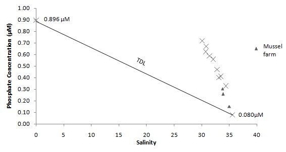
Fig8(b). Estuarine mixing diagram for Phosphate showing the theoretical dilution line
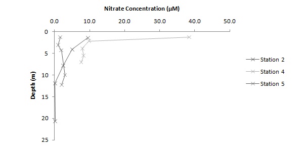
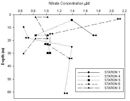
Fig9(a). Vertical profile of Nitrate vs depth for stations sampled
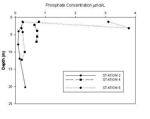
Fig9(b). Vertical profile of Phosphate vs depth for stations sampled
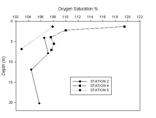
Fig11. Vertical profile of Dissolved Oxygen vs depth for stations sampled.
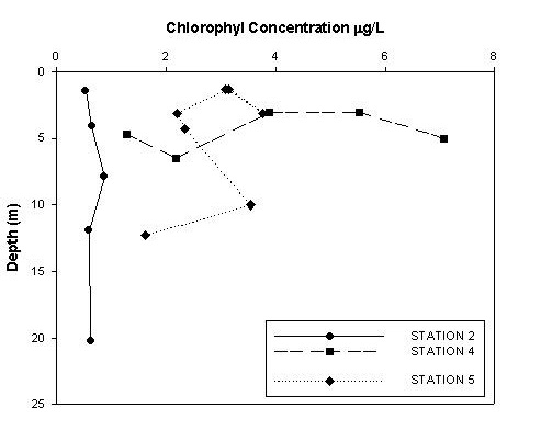
Fig12. Vertical profile of Chlorophyll a vs depth for stations sampled. |
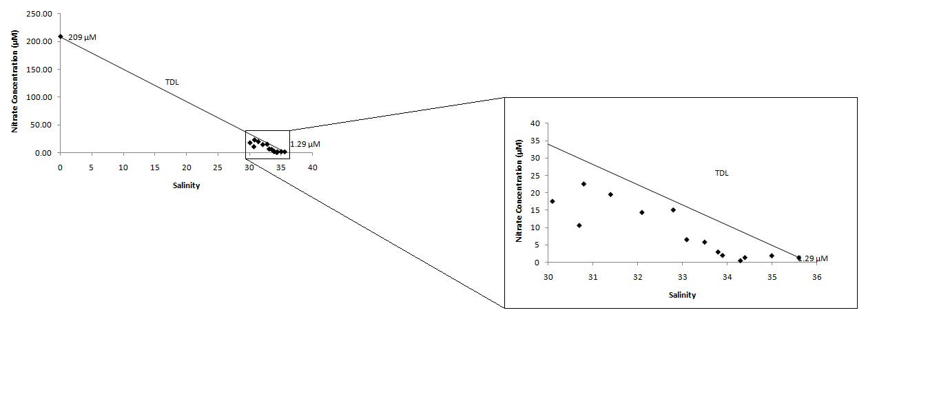
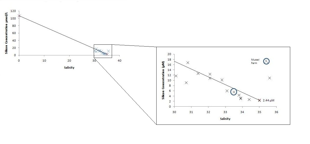
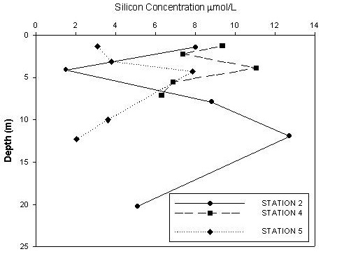
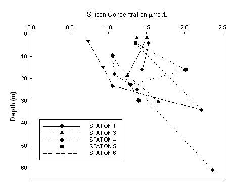
Analysis: In the horizontal profile taken of the estuary, the estuarine mixing diagrams (EMD) for the three nutrients show varying types of behaviour. The salinity range covered by sampling was 30 to 36 and the riverine end member with a salinity of zero was collected separately. All of the nitrate concentrations are below the theoretical dilution line (TDL) (Fig8(a).) indicating removal of this nutrient in the estuary. At the seaward end member, a concentration of 1.29 µM was recorded and 209 µM of nitrate were recorded for the riverine end member. This suggests that nitrate is behaving non-conservatively within the estuary, all of the other recorded points fall below the TDL suggesting removal of nitrate from the system by means other than mixing/dilution. However, when riverine end members were compared with Group 10’s data, the nitrate value was almost twice the amount at a concentration of 404 µM. This would affect the gradient of the TDL suggesting that nitrate would be in fact behaving very non-conservatively within the estuary. All of the phosphate concentrations (Fig8(b).) are above the TDL indicating an addition of this nutrient within the estuarine system. The most seaward end member recording 0.08µM and the riverine end member is shown to have a concentration of 0.89µM. Phosphate TDL also shows non-conservative behaviour with all of the seaward end members falling above the TDL suggesting addition of phosphate within the system. This could be due to sewage works or pesticides. The silicon (Fig8(c).) samples are distributed on both sides of the TDL, indicating areas of addition and removal of this nutrient within the estuary. The most seaward end member concentration is 2.44µM and the most riverine is 107µM. Silicon is behaving non –conservatively with depth at each station. This could be explained by biological utilisation however, there is little evidence of phytoplankton within the estuary at this time therefore suggesting another reason. The flow rate of the river could cause addition or removal of the silicon to the estuary depending on the amount of biological utilisation at the time. There has been little rainfall over the last few months which affects flow rate, this could be the reason for variable concentrations (Sigleo and Frick, 2007). Vertical profiles of the nutrients (Figure 9(a).) shows the profile for Nitrate at station 4 with the largest decline being between surface and approximately 3m (Δ 30µM). When comparing this figure to the salinity profile at this station it is apparent that there is more freshwater input at the surface which could be agricultural run-off and therefore contain high nitrate levels. Station 4 shows the highest concentrations of nitrate and phosphate taken in the vertical especially in the surface 5m. Station 2 (the most seaward end) shows the next highest surface nitrate concentrations which decreases with depth whilst station 5 shows the lowest surface concentration which are relatively well mixed with depth. The phosphate profiles (Fig9(b).) follow a similar trend with depth as the nitrate concentrations but all three stations show an initial decrease in concentrations at the sub-surface level and then show slight fluctuations throughout the remainder of the water column. The phosphate concentrations at station 4 are significantly higher than the other two stations, as station 4 is the most riverine sample collected this could be explained by land run-off (eg. Phosphate containing fertilisers) causing enrichment of the water column. Phosphate concentrations are generally low in the water column which can be reflected by the profiles at stations 2 and 5. The silicon profiles (Fig9(c).) for the different stations show variation with depth. Stations 2 and 5 show similar trends with concentration peaks occurring at depth below the surface, also within the surface 1-3m the silicon concentration experiences a sharp decrease. Station 4 differs from this by the surface concentration being low, significantly so in comparison with the other two stations, and then experiencing a concentration maxima at approximately 5m. The profiles do not demonstrate the expected behaviour for silicon concentration in an estuary and this is hypothesised that this may be due to analytical error as can be seen in the method section the analysis was carried out incorrectly. This would seem to explain the graphical representation but when comparing data with other groups for this nutrient, concentrations can be seen to vary with depth in a similar fashion. Values in the surface layer for dissolved oxygen % (DO) (Fig11.) are highest at the station closest to the head of the estuary (Station 4, 119.5%) (Fig. 1D), this trend follows with the chlorophyll a concentrations (Table3.) which coincides with the highest phytoplankton count (Table4). Stations 2, 3 and 4 show a general trend of decline in DO% with depth. This is most likely due to more organisms being present in the upper part of the water column and therefore DO% usage will be greater. The chlorophyll a concentrations at stations 4 and 5 show spiking with depth while the concentrations at station 2 show relative homogeneity (Δ ≤0.3µg/l). The largest chlorophyll spike is at station 4 (6.5µg/l, 2.18m), this coincides with the greatest decline in DO% (Δ 10%). The DO% at this station can be seen to be relatively homogenous beyond 4m. This suggests that there is a high DO% usage throughout the first 4m which links to the spike in chlorophyll concentration therefore suggesting an abundance of phytoplankton, which is probably due to more nutrients being available to the phytoplankton by enrichment of the water column. Station 5 shows a spike in chlorophyll concentrations at 10m depth (3.5µg/l). The vertical profiles of Fig 12 shows chlorophyll a concentrations are reduced throughout the water column with distance from the head of the estuary. This is evident in the horizontal profile taken (Table3.) which shows an over all reduction in chlorophyll concentrations with distance from the head. Due to the countryside area surrounding the Fal estuary being of high agricultural importance, run-off from the land into the estuary could lead to nutrient enrichment and eventually eutrophication. Using chlorophyll a concentrations as a measure for eutrophication one would look for values of ≥10µgL-1. The highest concentration of chlorophyll recorded in this data set does not exceed 8µgL-1 even at the head of the estuary where the concentrations were highest thereby suggesting that the area is currently not eutrophic. Mussel farm A water sample was taken immediately down stream of the mussel farm to investigate any change in nutrient input or output into the surrounding water. First expectations were that some additional input from the farm were to be expected due to increased input of faecal and detrital matter released from the harvesting and grading (cleaning) processes taking place on the farm before and during sampling. A possible phosphate increase was expected and could be explained by build up of faecal matter around the ropes on which the mussels grow, which is released when the mussels are harvested. However after a review of the lab data all the nutrient levels for the mussel farm were in line with other samples taken on the estuary and the respective TDL’s. This lack of increase in the mussel farm sample could be explained by the fact that the nutrients may not have had enough time or have been under the correct conditions to change from particulate to soluble state. Another hypothesis is the fact that due to the vast amount of nutrients and water flux through the farm from tidal flow means that significant removal or addition from the farm processes are insignificant and diluted to the extent that differences are undetectable. |
Fig8(a). Estuarine mixing diagram for Nitrate showing the theoretical dilution line
Fig8(c). Estuarine mixing diagram for Silicon showing the theoretical dilution line
Fig9(c). Vertical profile of Silicon vs depth for stations sampled. Table3. Chlorophyll concentrations with horizontal data points with graphical representation
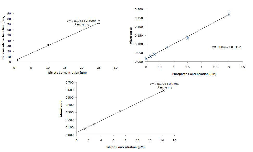
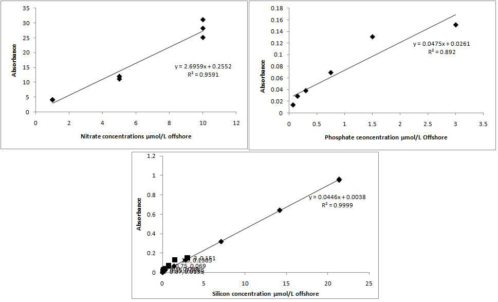
Fig10. Calibration standard for Nitrate, Phosphate and Silicon.
|
||||||||||||||||||||||||||
|
Biological: Methods: From the horizontal profile samples taken, 60ml of seawater was forced through a glass fibre filter with a syringe for chemical analysis. The filter was then placed into a dark glass bottle with 6ml of Acetone ready for lab analysis of chlorophyll concentrations. From the vertical profile samples, taken in Niskin bottles on the CTD, 100ml of surface estuarine waters were added to sample bottles containing Lugols iodine solution to fix phytoplankton to enable lab identification. A 200µm net with a 50cm diameter was towed behind the vessel just below surface for five minutes at two sites and the distance recorded. The 500ml sample bottles had 5ml of formalin added to fix the sample for identification. The net did not have a flow meter or propeller. |
||||||||||||||||||||||||||||
|
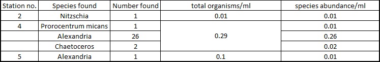
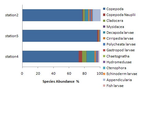
Analysis: Phytoplankton growth is controlled by a combination of factors, a maxima is dependent on hours and intensity of irradiance, temperatures, as well as available nutrients (nitrogen, phosphate, silicate) (Widdicome et al., 2009). The greatest abundance of phytoplankton out the stations sampled was at Station 4 (Table4.), the dinoflagellate, Alexandria, was the most prevalent genus (0.26cells ml-1). Dinoflagellates are all motile having two flagella enabling an efficient migration vertically through the water column to locate nutrients at depth when surface nutrients become depleted (Lewis and Allen, 2009). Station 4 shows the highest concentrations of nitrate and phosphate of the three stations, both nutrients depleting greatest at 3m depth which coincides with the highest chlorophyll a concentration for the station, suggesting that the nutrients are being depleted by the phytoplankton. This would correlate with the highest DO% at station 4 but not account for the 10% decline from surface to 3m. One would suggest that the zooplankton would be in greatest abundance where chlorophyll is hence, the decline in DO% is due to utilisation by zooplankton and possibly microbial decomposition. This is not observed from the collected data with the numbers of zooplankton being nearly identical throughout the estuary and not reflective of any maxima observed in chlorophyll and DO%. Location does not seem to be having a profound effect on the zooplankton abundance, nor any changes in phytoplankton. Copepods are the most abundant species (Figure13.) by a significant percent with other species making up a very small percentage of the sample. Whilst station 4 shows the highest abundance of phytoplankton (0.29ml-1), the abundance of zooplankton in comparison and lack of diatoms indicates that there has been a bloom of phytoplankton and the system is now in the stage of zooplankton succession. A minimal abundance of diatoms were recorded (0.01ml-1) indicating that this more valuable food source has been consumed primarily leaving the less nutritious dinoflagellates (McQuatters-Gollop et al., 2007; Geider et al., 1997).
|
Table4. Phytoplankton species abundance at stations sampled.
Fig13. Zooplankton species abundance at stations sampled. |
|||||||||||||||||||||||||||
|
Summary To summarise, we found that the Fal Estuary is more partially mixed than well mixed at this time of year and that the mixing processes are relatively tidal dependent as there is a low freshwater input. The ADCP data suggests a two layered water column developing towards the head of the estuary supported by the CTD profiles. All nutrients measured, were seen to be behaving non-conservatively within the estuary with nitrate being removed from the system and phosphate being added. Silicon behaved uncharacteristically for an estuary like the Fal and would need further study to determine the cause. The relationship between nutrients and plankton is complex and only shows trends at the more riverine end of the estuary. Though location has some effect on phytoplankton it does not appear to affect the numbers or species abundance of zooplankton in a significant way. As stated previously the Fal is a tidally dominated estuary and any defining features have been shown to be dictated by this. |
||||||||||||||||||||||||||||
|
|
|
|
|
|
|
|
| Offshore | ||||||||||||||||||||||||||
|
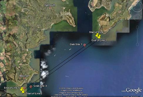
Introduction On 02/07/2010, R.V. Callista headed offshore from Falmouth on a south westerly heading with an aim of sampling the physical, chemical and biological parameters of the coastal waters and comparing how they vary with distance from the coastline (Table5). The main aspiration was to discover the location of the tidal front and to take measurements in the water column on either side of the key parameters to see how the water properties differ. Tidal data was checked for the day to maximise sampling opportunities. Multiple data collection equipment on board R.V. Callista allowed vertical profiles to be sampled at designated locations and for the surface temperature to be monitored as an indicator of the front location. Aims
Method An initial CTD profile was completed at Black Rock at the mouth of the Fal to enable the data to be compared to the seaward end analysis from the estuarine boat work. A T-S probe was used as Callista left Carrick roads to head offshore to detect any changes in temperature that would suggest an indication of the front. When these changes were seen the CTD was deployed and water samples were taken for further evidence. When the front was identified samples were taken to see if significant stratification could be seen. The furthest site was approximately 9 nautical miles from the shore. The final samples were taken close into shore to hopefully see a significant change in parameters for the coastal well mixed area and the frontal stratified area. CTD, Niskin bottles, Dissolved oxygen samples, light data and nutrient samples were collected using the same procedures as highlighted for the estuarine boat work. The same biological and chemical analytical methods were also used for processing the samples. A bongo plankton net was used offshore that collected a double sample one using a 100micron mesh and the other a 200micron mesh, this also allowed samples to be collected with depth in the frontal area to see how the fauna are varying in this area. Equipment used: CTD rosette, Niskin Bottles, T-S probe, Secchi disk, plankton net and bongo net, ADCP.
PSO: Joanna Wooles |
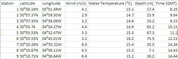
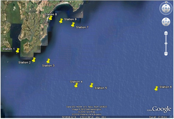 Table5. Location and parameter values for offshore stations.
|
|||||||||||||||||||||||||
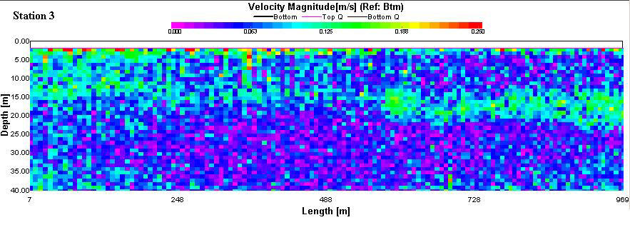 Fig14. Velocity magnitude plot for Station 3
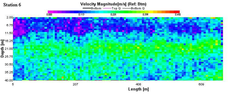
Fig15. Velocity magnitude plot for Station 6
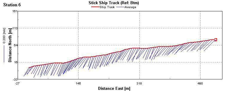
Fig16. Stick ship track showing flow direction for station 6
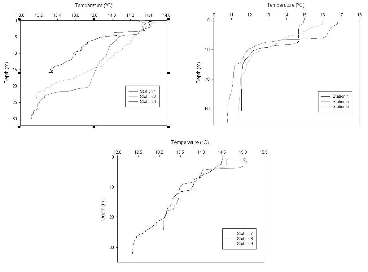
Fig17. Temperature depth profiles for offshore stations 1-3, 4-6 and 7-9
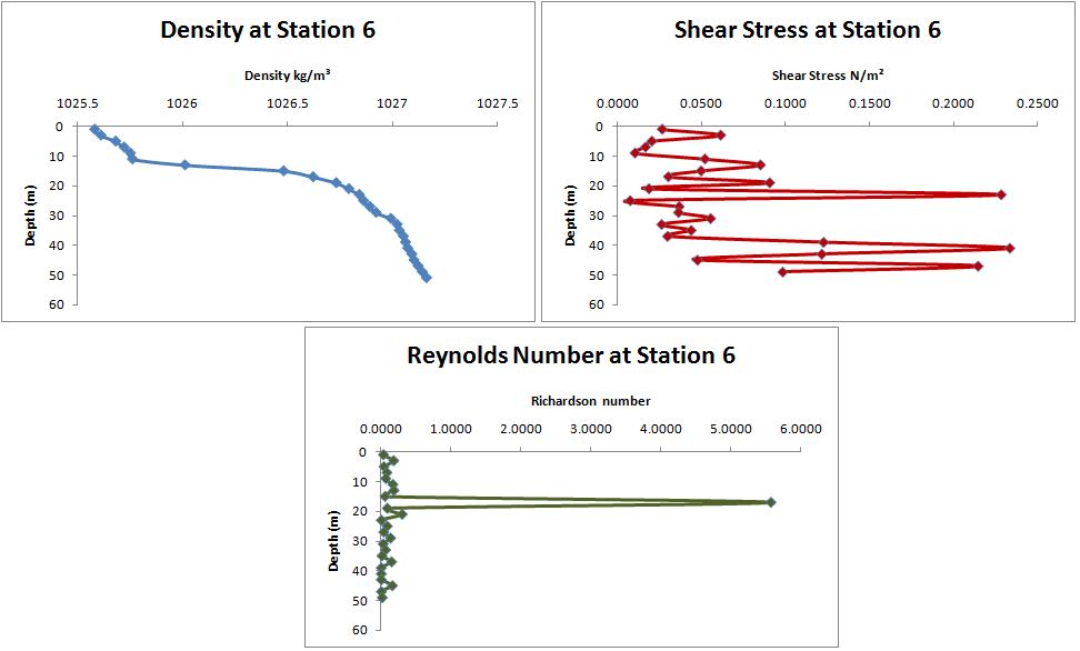
Fig18. Change in density, shear stress and Richardson number with depth at station 6
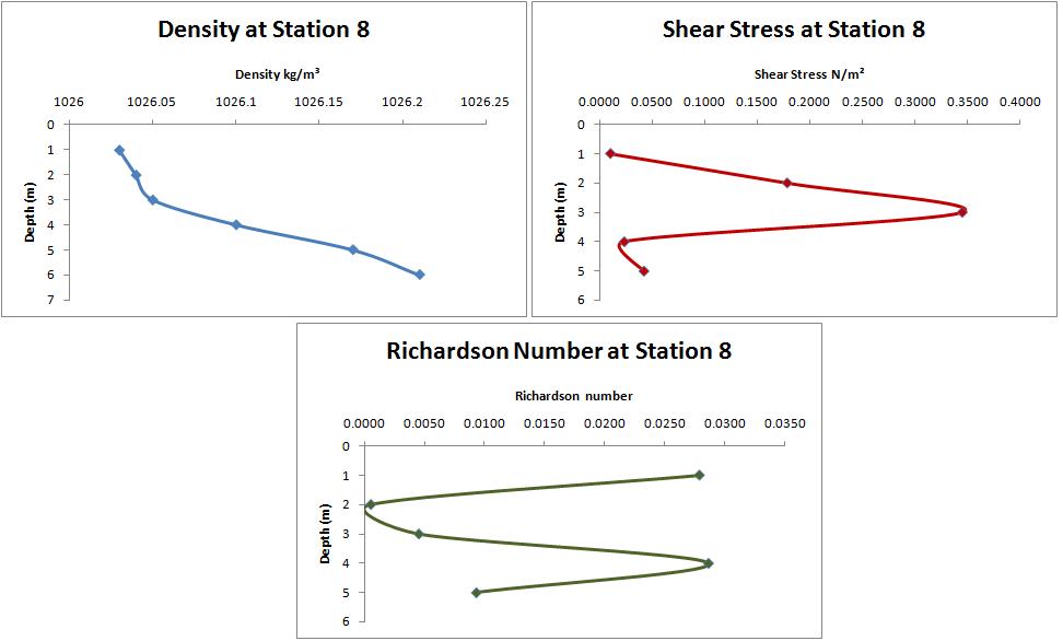
Fig19. Change in density, shear stress and Richardson number with depth at station 8.
|
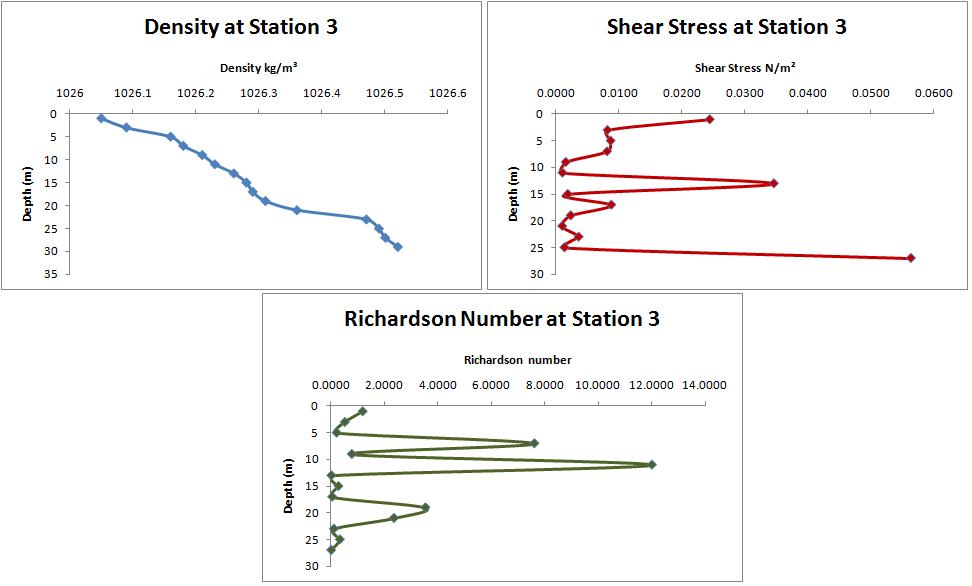
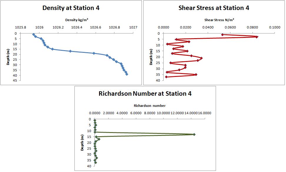
Physical Analysis All of the salinity profiles (Fig20.) show relatively little variation with depth. Therefore in offshore waters it is the temperature (Fig17.) which is indicative of mixing in theses vertical profiles. Stations 1 and 2 show weak thermal stratification with depth and no distinct thermoclines suggesting a degree of mixing indicative of coastal waters. The mixing is probably due to a decrease in depth of the seabed allowing greater tidal and wind mixing influence over thermal stratification. Station 3 shows two relatively weak thermoclines, the first at 5m depth and the second at 22m depth breaking the water column into three mixed layers. Stations 4, 5 and 6 show the highest Sea surface temperatures (SST) of the stations sampled; all three show strong stratification with thermoclines. Station 4 shows a strong thermocline at 19m depth showing a Δ50C over 1m. This is indicative of a seasonal offshore vertical profile of the water column, whereby the weak tidal mixing is not strong enough to overcome the solar radiation heating of the surface waters causing stratification. Station 6 shows a similar trend, whilst the thermocline at station 5 spans approximately 20m and Δ40C. Stations 7, 8 and 9 show trends comparable to those of stations 1,2 and 3. This is expected since these stations are closer to the coast and therefore subject to coastal mixing processes ie. tidal mixing. ADCP data analysed using WinRiver looking at Velocity magnitude, Average backscatter, Velocity direction and Stick ship track plots. The ADCP was used to aid locate and track the front from the Fal estuary. This was done by using backscatter to identify increase in zooplankton and ships track to look at change in flow direction indicating eddies. Station 1 shows SE flow with a 0.2ms-1 average throughout the water column. The ships track plot also shows this unidirectional flow. The backscatter shows no significant detail apart from relatively high backscatter patches which could be due to mixing from the ships props where the track moves in a loop. Transit to station 2 shows very similar values to station 1 with average flow increasing from 0.2 – 0.3 ms-1. At station 2 there is an average NE flow at the surface changing to average SE flow towards the bottom. The flow decreases towards to bottom from 0.4 – 0.2ms-1 indicating sheer flow from the bottom up. There is also a backscatter signal between 5 and 10m, this is most likely due to zooplankton. The CTD data shows a well mixed water column so sheer can be said to be from tidal flow. Transit to station 3 (Fig14.) shows an increase in surface velocity to 0.45 ms-1 and a corresponding change in flow direction below this point. At this boundary point there is an increased backscatter signature. On station there is a decrease in surface flow to around 0.1 ms-1 with a 0.15 ms-1 layer between 15 and 20m corresponding to a change in the velocity direction and backscatter plots with a change in 1 degree from surface to bottom shows on the CTD data. This related this to a possible beginning of the front. Transit to station 4 shows unidirectional S slow and an increased velocity layer corresponding to increased backscatter, this transit was around mid-tide. Station 4 and 5 shows increase in flow to 0.25 ms-1 and a difference in flow direction in the surface 10m to the rest of the water column possibly due to increased wind speed to around 4.6 ms-1 causing mixing. The backscatter shows a peak below this layer which matches the beginning of the thermocline on the CTD data. Transit to station 6 again shows relatively unidirectional flow at depth however the velocity magnitude plot shows an increase flow magnitude between 20 and 40m. There is a slight change in flow direction coinciding with a decrease in flow velocity (Fig15 and 16). The surface has increased flow velocity and around 90 degree difference in flow direction to the deeper water which may be due to an increase in wind speed to around 6 ms-1. At station 6 there are similar properties to the transit with the increased flow band at 12 and 26m. The CTD data shows a thermocline with a 6 degree temperature change starting at 12m, so the change in velocity could be due to buoyancy differences in the water. Half of the transit to station 7 is not reliable due to the boat travelling too fast to give accurate data. The other half shows increased flow velocity to 0.35 ms-1. Station 7 shows a unidirectional flow of around 0.125 ms-1 with increased backscatter in the surface 10m. The CTD shows increasingly mixed water as the boat moved towards the shore with a weaker thermocline. This station was taken at slack water and so could help explain the presence of the weak thermocline so close into the shore. The data for the transit to station 8 is too noisy and unreliable as the boat was travelling at speed. The CTD at station 8 shows a weak thermocline and ADCP showing weak flow with varying direction. Transit to station 9 shows similar properties to station 8 with increased backscatter in the surface layer around 5m possibly due to wave reflection from the shore. On station ADCP again shows similar data to station 8 with no significant flow velocity, this station was taken just after low water and so relates to slack water. Station 3 is located approximately 2.5 nautical miles from the mouth of Carrick Roads. Density in the water column is stable and as the depth increases the density also increases however this is only small (0.48 kg/m³) (Fig21). Shear stress is high at the surface due to wind stress and at the bottom due to stress against the sea bed due to tidal action. The Richardson number shows there is a stable layer of water at 10m with a well mixed layer at 13m. The friction and turbulence between these two layers causes a high shear stress at 13m depth. Two more unmixed layers are seen at 7m and 19m which could be due to currents flowing throughout the water column. At station 4 a pycnocline is seen from 10 – 20m with an increase in density of 1.04 kg/m³. There is high shear stress at this depth (Fig22) and the Richardson number is also high showing that there is a layer of very stratified water. Separate mixing is present above and below the pycnocline but there is very little interaction across this layer of stratified water. This would indicate passing the tidal front and entering offshore seasonal stratified waters. Station 5 (Fig23) was measured further offshore than station 4 though shows similar trends suggesting that the frontal system extends to this point and that the water column is still highly stratified. The location of the tidal front in the western English channel is highly dependent on tidal and wind mixing processes and can be defined by the equation E = log10+ε (Pingree et. al., 1978) where ε is the tidal energy dissipation per unit mass. Directly offshore from Falmouth the E values are <-2 showing easily stratified waters but close to this region, just off the lizard point, is a region of transitional waters where stratification is easily broken down by wind mixing and movement of the front is more likely making it quite hard to define in this region. Station 6 is the furthest station away from the shore at 8.6 nautical miles from the land. This station shows very similar results to station 4. A strong density gradient is seen from 10 – 20m. This highlights the pynocline with a range of 1.17 kg/m³. Again shear stress is seen at this depth and the Richardson number has a huge increase between 10-20m. This is suggesting that this area of the water column is experiencing strong stratification, though the water above and below this site appears to be well mixed. Station 8 is taken at 0.2 nautical miles from the shore as a comparison to the offshore sites (Fig19), to see how the wind stress and bottom stress form tidal action causes a well mixed water column. A gentle density gradient with a range of 0.18 kg/m³ can be seen over 6m. Richardson number is seen to be high at the surface and another layer of stratified water at 4m depth. This could however be due to bottom stress as the water was only 7.0m deep. When comparing this data to that of the CTD profiles it is apparent that at station 8 the column is relatively well mixed and showing no thermocline when at stations 4, 5 and 6 where the richardson numbers suggest stratification this is supported by strong thermoclines. |
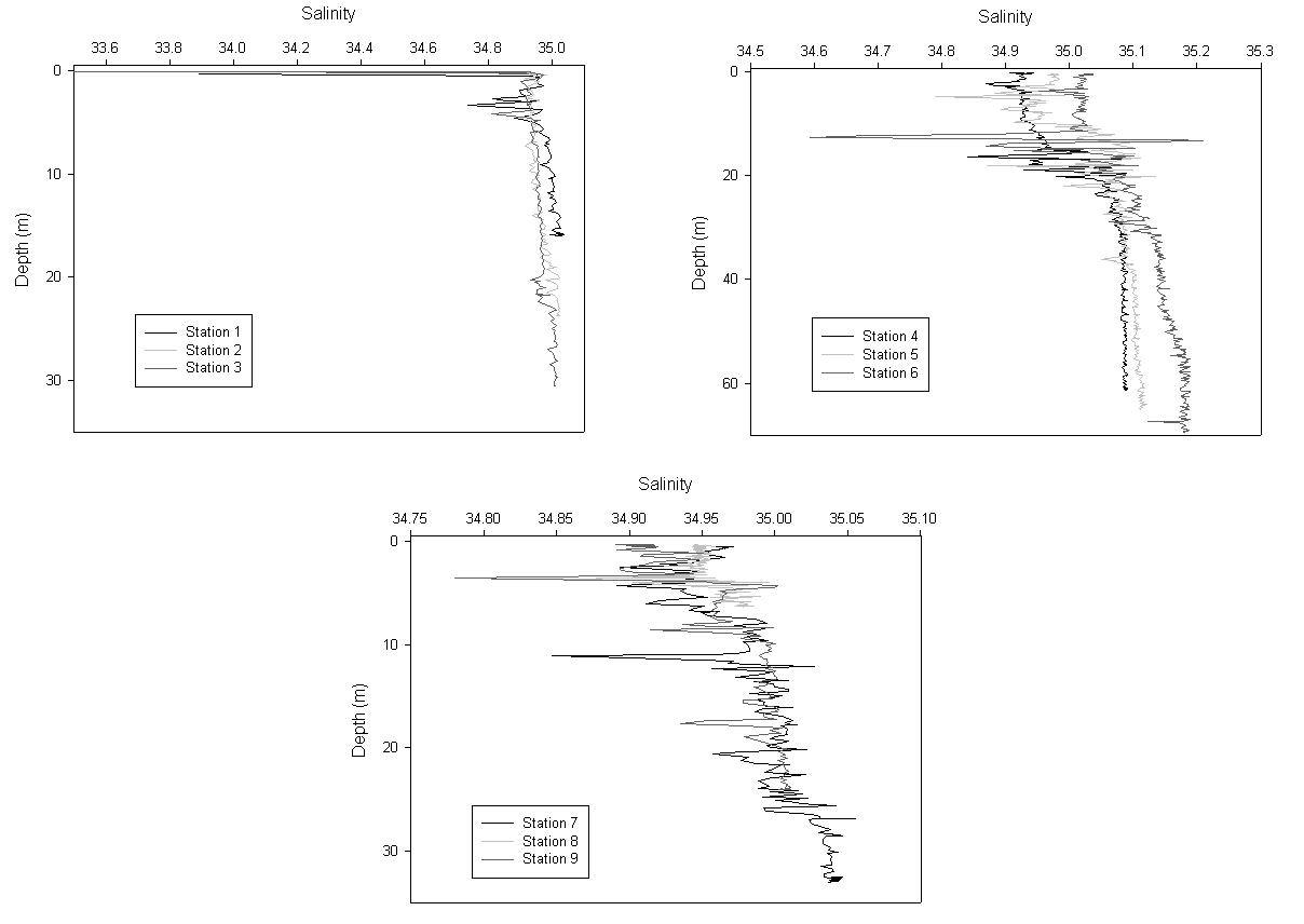 Fig20. Salinity depth profiles for offshore stations 1-3, 4-6 and 7-9.
Fig21. Change in density, shear stress and Richardson number with depth at station 3
Fig22. Change in density, shear stress and Richardson number with depth at station 4.
Fig23. Change in density, shear stress and Richardson number with depth at Station 5
|
||||||||||||||||||||||||
Fig24. Calibration standard for Nitrate, Phosphate and Silicon. |
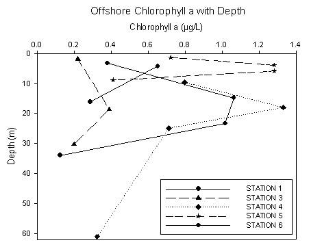
Chemical Station 1 (Black Rock) showed an increase in concentration with depth and the levels at 4.25m were the same as those than at 4.2m at station 5 offshore at 1.39µM. At the headland station 3 there is a constant decrease with depth as the nutrients are subject to biological take up. The first sample at offshore station 4 was taken at 9.61m and data shows a gradual increase in concentration to sampled depths of 61m as the nitrate (Fig27.) is returned to the water column via recycling and sinking. Stations 5 and 6 show similar profiles of depletion in the upper 15m of the water column followed by replenishment with depth. This is to be expected as after passing the front into seasonally stratified waters the upper water layers are expected to be nutrient depleted due to high phytoplankton abundance with the lower layers being periodically replenished by the deep, cold, nutrient-rich water at the bottom of the water column (Pingree et. al., 1977). Station 1 (Black Rock) showed an decrease in concentration with depth and the levels at 4.25m were 11% higher than at 4.2m at station 5 offshore (Fig26.). At station 3 there is a constant decrease with depth as the nutrients are subject to biological utilisation through the light-rich sub surface waters. An increase then occurs after 20m as silicate is returned to the water column through recycling and mixing. The first sample at offshore station 4 was taken at 9.61m and data shows a gradual increase in concentration to sampled depths of 61m. Unlike nitrate concentration Stations 5 and 6 show differing profiles. Station 6 shows depletion at surface and increase with depth. Station 5 shows comparable initial increases but has higher concentrations at the 16.0m sample. This could be due to sampling/analytical error or a deeper community of diatoms that were not recorded from the net trawls. Results from chlorophyll sampling at 14.7m and 23.3m show an increase in concentration (µg/L) supporting the hypothesis that there could be an increase in phytoplankton abundance. After completing the chemical analysis on the water samples with regards to phosphate it was evident that the amounts of phosphate present were below the detection limit which for phosphate is 0.03µM. Due to this no graphical analysis has been completed on the phosphate data as any results would prove inconclusive. This could be due to excessive amounts of utilisation or lack of efficient mixing throughout the water column. Station 1 taken at Black Rock shows dissolved oxygen (Fig25.) to be well mixed throughout which follows a similar trend to the chlorophyll at this station. Stations 4, 5 and 6 show the most interesting results as all three show spikes of dissolved oxygen and chlorophyll at an approximate depth of 10-20m. This would suggest high photosynthesis rates and abundance of phytoplankton, this could highlight the area of water where light irradiance is still high but the deep enough for enrichment of nutrients to be occurring to support the plankton growth. For station 6 this hypothesis is supported by high nitrate content, though nutrient data for the other stations have proven to be inconclusive in supporting this. After peaking sub-surface both chlorophyll amounts and dissolved oxygen ( decrease with depth as is expected when light decreases.
|
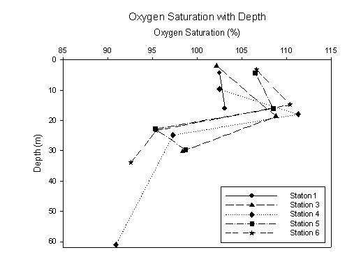 Fig25. Depth profile for oxygen saturation for offshore stations 1, 3-6
Fig26. Depth profile for silicon for offshore stations 1, 3-6
Fig27. Depth profile for nitrate for offshore stations 1, 3-6 |
||||||||||||||||||||||||
|
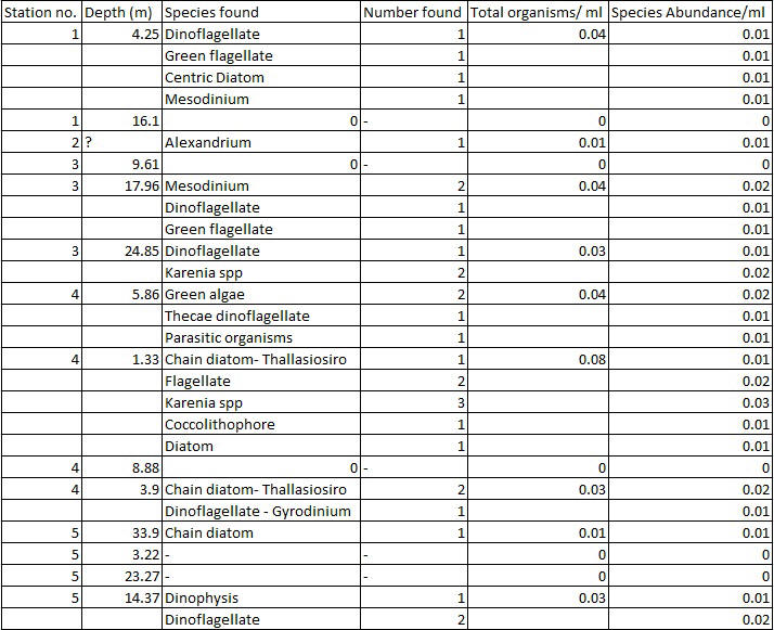
Table6. Phytoplankton table with species abundance
Fig30. Chlorophyll a depth profile for offshore stations 1,3-6. |
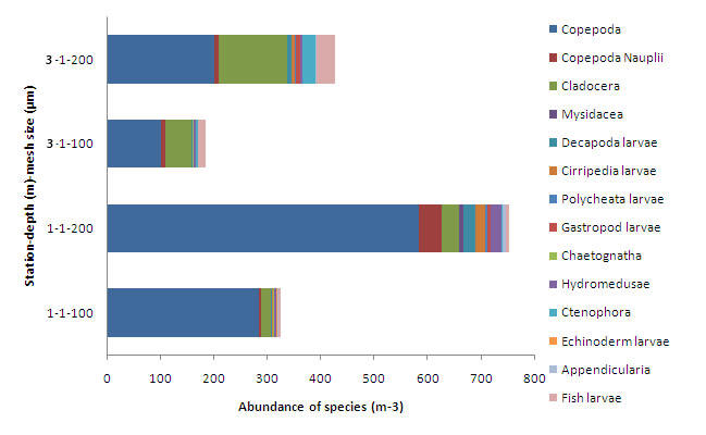
Biological A 200µm net at Station 1 shows the greatest abundance of zooplankton of the samples taken (750m-3) of which copepods are the dominant species. Primary production abundance at this station shows 0.04cells/ml at 4.25m depth and 0 cells at 16m depth. This is the station closest to land, therefore, it is possible that due to anthropogenic inputs increasing coastal nutrients, a relatively large bloom of phytoplankton (Table6.) has been succeeded by a zooplankton bloom, the greater the abundance of prey the greater the abundance of predator. In tidal front systems, the tidal and wind mixing are typically the defining features for its position and any subsequent movement, the coastal waters surrounding the Fal are areas where light is not a limiting factor due to lower turbidity in the water column and therefore during a spring tidal cycle the primary productivity of the frontal area is increased due to replenishment of nutrients through mixing (Ragueneau et. al., 1995). When sampling offshore the tidal cycle was neaps and therefore could be another reason as why there are low amounts of phytoplankton and therefore production in the collected samples. The zooplankton with depth profiles (Fig29.) at stations 4 and 6 show the greatest abundance between 0 -15m. Unlike the bongo samples, both copepoda and copepod nauplii are the dominant species suggesting an availability of food. Comparing the chlorophyll data (Fig30.) for the two sites with the zooplankton shows that the zooplankton are located in the same area as their prey, chlorophyll concentrations decrease at both stations beyond 20m depth (probably due to light saturation at depth). The dissolved oxygen trend at these two stations shows a trend that corresponds with the chlorophyll concentration levels. The data needs to be compared over a temporal scale to observe if the position of the zooplankton is due to diel vertical migration.
|
Fig28. Abundance of zooplankton species at the surface of station 1 and 3 mesh sizes 100 and 200 microns
Fig29. Abundance of zooplankton species at station 4 and 6 from depth
|
||||||||||||||||||||||||
| Summary The aim of the boat work was to try to identify the location of the tidal front and how the parameters of the water column change on either side. Although the front was not identified on a micro-scale the water becomes strongly stratified at stations 4, 5 and 6 suggesting that the front has been passed and seasonally stratified waters have been reached. Tidal mixing and light intensity are factors that can define the front location and any subsequent movement; these can also have a major impact on the phytoplankton growth. All physical, chemical and biological parameters support the indication of the frontal system, with the physical data being particularly conclusive. |
||||||||||||||||||||||||||
|
|
|
|
|
|
|
|
| Geophysics | ||||||||||||||||||||||||||||||||||||||
|
Introduction To conduct a benthic survey using the equipment available on board the RV Explorer to provide information on habitat and sediment types in the Fal Estuary area. Aims & objectives To plot the benthic community between the Fal estuary and the river Helford within the SAC area. Starting from one edge of boundary across the middle of the site using two parallel transects, observing areas of interest on the first to highlight areas for grab samples on the return.
PSO: Ben Edwards |
 |
|||||||||||||||||||||||||||||||||||||
|
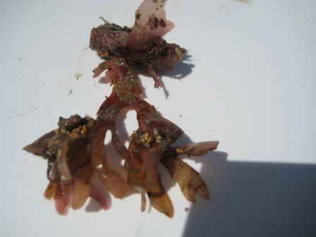
Method and equipment A Tow fish attached to a 5m line was deployed and towed at a constant velocity of 4.4knots. The Side scanner set at 450kHz frequency emits a pulse which is absorbed, or reflected back to the transmitter. The varying backscatter produces changes of colour from white to black, black representing higher reflectance indicating denser sediment types and elevated or lowered bed forms. White represents shadows and increased absorbance normally associated with softer sediment types. The backscatter data from the transects was relayed to an on board computer where it was observed in situ to determine areas of interest, the latitude and longitude were recorded to enable identification of areas to be used for videography and grab samples. Simultaneously ADCP (1200 kHz frequency) was observed to assist in determining the sediment composition through flow rates and backscatter. Three main areas of interest were determined, one was thought to be Bedforms, and the other two identified on the side scan profile by a dividing line (one area darker than the other) close to the mouth of the Helford, one of these sites was originally believed to be a seagrass location. A video camera mounted on a scaffolding frame, deployed via the crane was lowered to the sea bed, images projected on a screen and recorded. The images were used to help identify the habitat and sediment type and any benthic fauna. The video camera was deployed at each of the three sampling stations. Whilst the camera is on board it is kept in a bottle of fresh water to prevent it from fogging. Due to there being no seagrass observed at the stations a 0.01m3 Van Veen grab was deployed using the ships Hiab crane to obtain samples of the seabed (the grab is deployed open and closes on impact with the substratum).The samples were identified as much as possible in situ and photographs taken for further identification. |
||||||||||||||||||||||||||||||||||||||
|
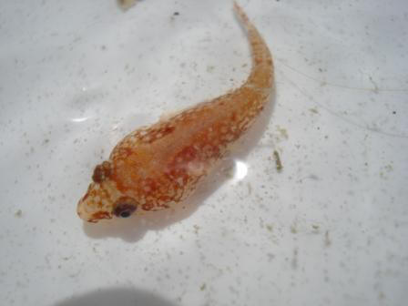
Fig31: Lepadogaster lepadogaster
Fig32: Chonurus crispus
Fig33: Pharus legumen juvenile |
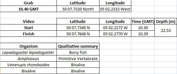
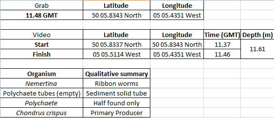
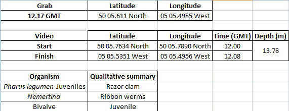
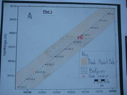
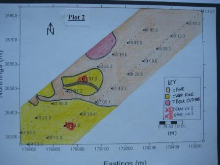
Results Station 1 Video 1 was situated on top of a bedform (Table7.). The video highlighted a high number of starfish throughout the area (28 spotted, including two brittle stars). Sediment was observed to be partially sorted as 95% of sediment of the grab was seen to be maerl out of this 99% were assumed dead (shown through live maerl being pink and deceased anything else). The video shows an estimate of 5% shell debris typically; ranging to 25% in areas. Macro algae in the area were seen to cover 2-10% typically and up to 85% in rare areas (shown through video analysis). A hermit crab was seen on the video footage. Shell debris was observed to occur in lines, this is assumed to be the lee side of the bedforms ripples. Almost all sediment was seen to stay within the sieves first two layers (2% in top layer, 63% in middle sieve) with a combination of smaller sections of maerl and broken shells in the smaller sieve section (1cm, 2mm and 1mm pore size respectively). Station 2 Macro algae were observed from video footage to cover 30% of the sea floor ranging from 10-50% in areas (Table8.). Macro algae was seen in two different species but there was not enough detail to identify further. Broken shells were seen at 40% average ranging from 10-70%, with no evidence of bedform patterns. Two crabs were seen on the video footage. The grab was observed to be well/partially sorted with fine sediment (84%) falling through all levels of the sieve, the sediment left in the middle sieve (10%) was seen to contain large biota and shell pieces followed by small biota with small shell fragments (6%) (pore sizes 1cm, 2mm and 1mm respectively). Station 3 Shell coverage was observed to cover 1% average of the sea floor, with cast forms in the sediment at regular intervals this could be formed by deposit feeding Polychaetes causing bioturbation (Table9). Two types of macro algae were seen to be in the area but they were of too low a frequency to warrant mention of being typical of the area. A decapod, hermit crab and a bony fish was seen but with too little detail to be identified to a higher degree. The sediment was quantitatively analysed to be well sorted with roughly 97% of sediment washing through all sieves indicating a size of less than 1mm, the other 2% was spread within the 1mm sieve with 1% within the 2mm sieve. Sedimentology Sediments in plot 1 (Fig34.) constitutes of largely dead Maerl beds, making up the top layer of sediments, as can be seen from the sidescan plot and from analysis of the grab samples. Maerl grows on St Mawes bank, in the Falmouth estuary, but it has been shown the maerl previously inhabited a much larger area. Bedforms can be see in the plot, ranging from a waveheight of 0.18m to 0.61m and a wavelength of 1.12m to 1.74m, and by using a bedforms characteristics table (Hughes, 2003), the bedforms can be characterised as small subaqueous dunes. It has been assumed that the bedforms have been created by tidal currents; however, it is also possible that these are storm event beds, and as such may have significant age (John Davis, 2010). Plot 2 (Fig35.) shows a significant boundary between fine and very fine sediment types, which is thought to be the edge of sediment deposition from the Helford estuary. Grab site 2 was taken as fine sediment, however, this may due to grab drift from the original position, as it was thought that grab site two and three would have similar sediment. Sediments around grab site two may also have been part of the very fine sediment body; however, it is possible current flows may have isolated this location as a small island. Sediments were analysed from grab sites for grain size. |
Table7. Location and organisms found from grab 1
Table8. Location and organisms found from grab 2
Table9. Location and organisms found from grab 3
Fig34. A benthic plot highlighting bedforms.
Fig35. A bethic plot highlighting potential seagrass site and change in sediment type |
||||||||||||||||||||||||||||||||||||
|
Analysis Starfish are regularly found at station 1 showing a high quantity of prey among the dead maerl as Starfish feed on bivalves, Polychaetes, small crustaceans and other echinoderms (BBC, 2005). The appearance of starfish at station 1 and not 2 and 3 suggests that there is a higher density of prey at station 1 than the other two. Bivalves generally survive and flourish in areas of course sediment rather than fine as they are generally filter feeders which get feeding filters clogged in areas of fine sediment. The appearance of the razor shell (Pharus legumen) at station 3 is an important indicator of the sediment type, the razor shell typically inhabits areas of sediment where silt is present (Yonge, 1959), the sediment type of station 1 causes the area to be uninhabitable whereas the sediment structure of stations 2 and 3 (low grain size) show silt within the area. Although no razor shells were found at station 2 the area is large and sample size low, the video would normally identify if a species inhabited the area however the species is too small to show up therefore it cannot be said that razor shells do not occur around station 2. Station 2 was observed to have a 30% average more macro algae than station 3. The sediment at station 2 was partial to well sorted whereas station 3 was seen to be well sorted with a higher percentage of very fine sediments (less than 1mm).This shows reasonable evidence to suggest that macro algae may be proportional to how well sediment is sorted and to the average sediment size. It has been seen that macro algae find soft sediments and mud which may be organically enriched least favourable for colonisation (Balata et al, 2007). This shows evidence for why there are less macro algae at station 3 than other stations. Amphioxus is a semi-motile cephalachordate which allows it to resuspend itself in the water column in case of sediment burial. It was present at station 1 in the Van Veen grab and not recorded at either station 2 or 3. As a filter feeding organism it is reasonable to suggest that this may be a result of sediment type. Sediment at stations 2 and 3 was observed to have 16% and 0% grain size above 2mm respectively; this shows a lower than 2mm grain size average which is small enough to clog a filter feeders apparatus disrupting the amphioxus’ energy budget making it unsuitable for the area (Dough et al,1999). Summary Having examined the grab samples in detail in terms of physical and biological properties it can be suggested that the type of sediment plays a key role in determining the type of organisms that are able to live in these locations. However, significantly more grab samples would be required to provide evidence for this statement. Furthermore, it has been discovered that it is difficult to determine specific biotopes with limited time and resources. |
||||||||||||||||||||||||||||||||||||||
|
|
|
|
|
|
|
|
| Summary of fieldtrip |
|
During the two week long field course data has been collected with regards to the influential parameters within the estuary, details of the surrounding benthic habitat and the features that define and change coastal fronts. St. Mawes Bank near mouth of the Fal estuary has the largest area of a living maerl biotope in England. Maerl deposits have been found in Carrick Roads and Falmouth Bay showing that maerl previously grew in those areas, though due to the strong tidal influence in the estuary and surrounding waters the dead maerl deposits could be transported a notable distance. The pumping of sewage into the Fal Estuary may cause eutrophication and has been known to in the past. This is known to have a negative effect on maerl growth as it causes competition of nutrients and light availability due to turbidity (UK marine SAC website). During the grab samples only very small amounts (0.5%) of living maerl was recorded in comparison to dead. Alexandrium was found in the phytoplankton samples collected in the estuary (though only a small amount), and is typically a sign of eutrophic waters. A key way of determining eutrophication is the chlorophyll level in the waters, from the data collected during the field course, chlorophyll amounts did not exceed 8µgl-1 (threshold for eutrophication is 10 µgl-1) and therefore suggest that the estuary is currently not eutrophic. When comparing the offshore data to the estuary data, phytoplankton in both systems are low and have been succeeded by a bloom of zooplankton suggesting the phytoplankton bloom has been missed in these observations. Due to this the primary productivity in both systems can be described as low, though from offshore samples slightly higher concentrations of phytoplankton were found. These levels will probably remain low until autumn when the stratification will break down releasing nutrients back into the system and cause a bloom in phytoplankton and primary productivity. Especially for the offshore work, detailed light data was not recorded or analysed. This is an important factor controlling many processes in the ocean and for further study would be interesting to calculate the euphotic depth and/or critical depth and compare/contrast this to existing data collected over the duration of the field course. |
|
|
|
|
|
|
|
|
| References |
Photos
|
|
|
|
|
|
|
|
|
| Disclaimer This website is the opinion of the group of students only and do not in anyway reflect the views of the NOC. |


