|
 |
Matthew Couldrey I am currently studying oceanography. In particular, I am interested in physical oceanography, but I also like various aspects of biology, chemistry and geology. I have not yet decided exactly what I want to do in the future, but broadly I would like to continue to do oceanography, especially fieldwork.
|
 |
 |
Becky Hemingway I chose to study oceanography due to its diversity in all science topics and I enjoyed investigating how they all interlinked with each other. My favourite parts involve mostly physical oceanography especially the weather side of this and seeing how it affects the oceans’ movement. I also really like helping with the navigation on ocean vessels to determine where to go. I hope to further study climate change and the affects it has on the planet. I have loved the oceans since I can remember and have a real passion for their future upkeep and how to save them for future generations |
 |
Karli Scherer I am studying Marine Biology and Oceanography at the University of North Carolina Wilmington. I am currently and studying at the University of Southampton on exchange.. I love the Invertebrates of the ocean, mainly Jellyfish and Sting Rays because of the graceful way they move and how simple the creatures really are. In the future I hope to work towards marine conservation and protecting those who may not be able to help themselves.
|
 |
 |
Jessica Amies I am currently studying Oceanography and am particularly interested in the interactions of the ocean with the atmosphere and climate. After finishing my degree I would like to travel and hopefully start a career related to the aspects of ocean science in which I’m interested. |
 |
Genevieve Elsworth Genevieve Elsworth is a second year geology student on exchange from Penn State University. She is interested primarily in the physical and chemical aspects of oceanography. In the future she would like to work in the field of environmental geochemistry. |
 |
 |
Jennifer Dean I am studying Marine Biology at the University of North Carolina Wilmington. I love everything about the ocean, but the area I am most interested in is marine mammal conservation. In the future I would like to travel the world, buy a sailboat, and lead my own research team. |
|
Erin Udvare Erin Udvare is a Marine Biology student at University North Carolina Wilmington and studied in Southampton for spring term 2010. Home is Milwaukee, Wisconsin where her mother and father still live with her dog, Cleopatra, and cat, Mr. Bigs. She is planning on attending graduate school in 2011 and going into conservation or biological oceanography.
|
 |
 |
Ted Present I am a third-year geosciences student from Pennsylvania State University. I plan to pursue a graduate degree in marine geochemistry because I am excited by the large-scale influence the oceans have on our world, and the power chemistry has to explain ocean-system processes over tremendous time and space scales. |
 |
Julia Haywood I currently study Marine biology and my main interests include mangroves and corals. I hope to do research on the mangroves in Florida for my dissertation work and possibly follow my Masters degree with a Ph.D. After I make it out of university into the real world I would like to be a field marine biologist and travel around the world where ever the work takes me. |
 |
 |
Zach Mazlan At the moment I am studying oceanography at Southampton. I look to further my experience by studying abroad for a year in North America. I am an avid diver and enjoy sailing. I hope to work for an offshore survey company in the future and travel the more remote areas of the world. http://www.zacharymazlan.com |
|
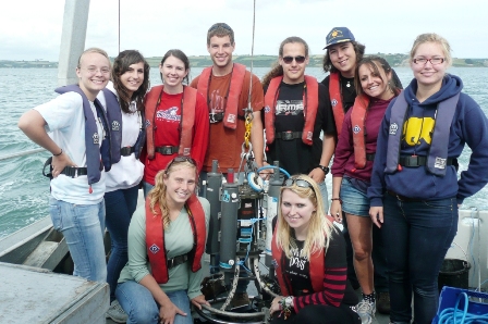
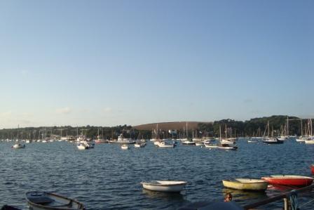
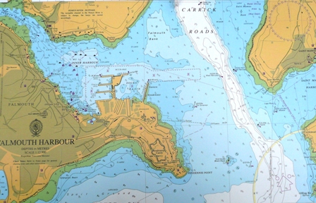
An investigation into the chemical, physical, and biological processes influencing the Fal estuary was undertaken by ten oceanography and marine biology students during June 2010. Located in the county of Cornwall the Fal estuary is England’s largest estuary and natural harbour. The estuary extends 18 kilometers inland from St Anthony’s Head and Pedennis Point to Tresillian and consists of an outer tidal basin (Carrick Roads) and inner tidal tributaries. The majority of the water within the estuary is contained in the outer tidal basin which is characterized by a deep channel with an average depth of 34 meters. Inland the channel shallows to an average depth of 12 meters near the mouth of the River Fal. The Fal estuary supports a variety of ecosystems including large areas of intertidal mudflats, subtidal sandbanks, and salt marshes. The Fal estuary is a ria formed during the last glacial maximum (approximately 10,000 years ago) due to tectonic subsidence and sea level rise. Tributaries of the estuary include the River Carnon, River Penryn, River Kennal, River Truro, Mylor Creek, Pill Creek, Penpol Creek, and Restronguet Creek. These tributaries drain areas of Carnmellis granite and Devonian carboniferous rocks. Despite the large number of tributaries freshwater influence is negligible and the estuary is influenced strongly by tidal mixing. Although tidal heights vary with location most areas of the Fal estuary are macrotidal with a maximum tidal height of 5.3 meters. Surface water temperatures range between 16 degrees Celsius in the summer and 9 degrees Celsius in the winter with an approximate salinity of 35 in coastal waters. |
 |
|
 |
The Fal estuary is designated as a Special Area of Conservation due to an impressive diversity of organisms and habitats. Areas of ecological significance in the estuary include mudflats, maerl beds, seagrass meadows, and subtidal mudflats. Ecosystems within the Fal estuary have been heavily influenced by metal pollution and nutrient inputs. Elevated levels of organic nutrients have been observed in the estuary due to the drainage of agricultural areas. Elevated levels of both nitrate have lead to eutrophication in some areas of the estuary. Elevated levels of tin, copper, lead, and iron are observed as a result of local mining since the Bronze Age. Significant metal contamination has resulted from the abandonment of the Wheal Jane Mine in 1992. The release of acidic metal laden water into the Fal estuary has resulted in elevated zinc and copper concentrations. The leaching of tributyl tin (TBT) from ship hulls has elevated levels above the EQS value of 2 ng/L. Sewage discharges, dredging, and oil release have also polluted the area. As a result of such contamination the Fal estuary has been designated as one of the most polluted estuarine systems in the UK. The biological, chemical, and physical characteristics of the estuarine system were investigated using four research vessels (Callista, Xplorer, and Bill Conway) and a variety of scientific equipment. A biological and chemical survey of the offshore and estuarine systems and a geophysical survey of benthic habitats will allow the behaviour of the estuarine system to be considered. |
|
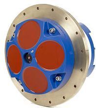 |
ADCP The ADCPs used aboard both Callista and Bill Conway are Teledyne’s Workhorse Mariner ADCPs with operating frequencies of 600kHz. The Workhorse Mariner is ideal for coastal research applications, being hull-mounted and has a range of 165m. The ADCP makes use of a 4 beam system to provide reliable, high resolution- low noise data. ADCPs are used for detailing subsurface water currents and finding organisms in the water column. The ADCP sends out 4 acoustic beams from its 4 transducers, which observe the returning signal to determine the direction and speed of currents. It can also indicate the positions of organisms in the water column such as large zooplankton groups. |
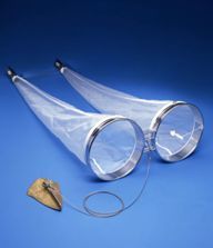 |
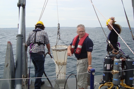
Bongo Nets The bongo net consists of two plankton nets of differing in soft mesh size mounted adjacent to each other. The mesh sized used were 100 and 200 microns. Each net has an independent collecting bottle attached at the cod-end to allow simultaneous collection of samples from each net. The bongo net is deployed from a vessel and towed horizontally at a constant speed, sampling at a fixed depth beneath the surface. The depth of sampling can be adjusted by varying the length of the towline. More complex models of bongo net may include depressor fins or weights to set depth and cylindrical fibreglass frames at the mouth to allow vertical trawls.
|
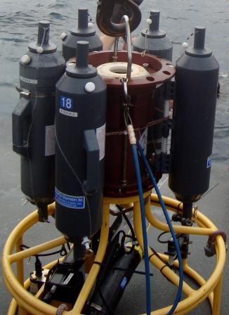 |
CTD Rosette The CTD Rosette is a collection of various oceanographic tools bundled onto a single frame. The pictured rosette (left) is one used aboard the Callista. The rosette frame supports interchangeable pieces of equipment, usually sensors and sample bottles. The sensors used include a thermosalinograph (for temperature and salinity), fluorometer (for chlorophyll), transmissometer (for turbidity), pressure sensor (for depth). All the sensors are affixed to the bottom of the frame and linked to an on-board computer which gives real time readouts of the various parameters they measure. Additionally, the CTD Rosette has an array of Niskin sample bottles which can be triggered remotely by the on-board computer. By coupling the bottles with sensors, the issue of blind sampling is avoided as fine features (such as thermoclines or chlorophyll maxima etc.) can be sampled by firing the bottles while observing the real-time sensor outputs. |
CTD Sensors -Transmissometer: A transmissometer is used to measure the turbidity of a sample. The device sends a narrow beam of energy, usually a laser, through the medium being sampled. A narrow field of view receiver is situated on the opposite side of the sample at a set distance. The amount of energy arriving at the detector is measured and used to quantify the amount of substance suspended in the water colum -Fluorometer: A fluorometer is a device used to measure certain parameters of fluorescence including the wavelength and the intensity of the emission spectrum after a sample is excited by a certain spectrum of light wavelengths. The amount of light passing through the sample is restricted by the electrons of the atoms, therefore an increase in atoms results in a decrease of transmitted photons. These absorbance measurements allows for the identification and quantification of fluorescing pigments in a sample. From this data chlorophyll concentration was determined. -Depth Sensor: Judging depth is done indirectly by observing water pressure. At depth, water pressure increases predictably. Depth sensors actually monitor these changes in pressure and use them to relate to water depths. -Temperature/Salinity Probe: Temperature is measured using a thermistor which is a resistor whose resistance varies with temperature and a platinum resistance system. The two mechanisms respond to temperature change and couple their outputs to give a quick response-high accuracy temperature reading. Conductivity is measured using two electrodes. From this data salinity can also be calculated by using conductivity data and correcting it for temperature and salinity.
|
|
 |
Valeport current meter This gives a real time current measurement as well as short to medium term autonomous deployments. This is especially useful for coastal and river measurements and can be used even on small boats. The numbers of impeller rotations are counted per second along with a single compass heading reading, this enables the East and North velocity vectors to be calculated. |
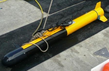 |
GeoAcoustics Sidescan Sonar This sidescan sonar equipment collects information on seafloor bathmetry as it is towed behind a vessel by emitting pulses. These pulses are reflected off the seafloor and the backscatter is recorded in slices as a time series which allows a picture of the seafloor to be built up. The instrument has dual frequencies (114 and 410 kHz) which can be switched between while the sidescan is taking place; the higher frequency setting has a better resolution but lower range than the lower frequency setting. The darker parts of the sidescan image have higher energy and therefore greater reflectance than the lighter parts which have lower energy, for example white areas are shadow zones.
|
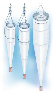 |
Nansen Closing Net (Vertical Plankton Net) The Nansen closing net or vertical plankton net is used to sample between defined depths. It consists of a plankton net with a vented collecting bottle at the cod end. It is equipped with a drawstring near the mouth, which when pulled closes the net, preventing unintended sampling at shallower depths when the net is retrieved. The net can be equipped with a depth sensor to allow for monitoring of depth. The net is lowered to the start depth and then raised up through the water column to the end depth. During this time, water flows through the net and plankton larger than the net mesh size (200 microns) are retained in the net. The drawstring mechanism is then triggered by the use of a messenger weight, which trips a catch releasing the primary haul lines and transferring the load to the drawstring. This in turn causes the mouth of the net to close. |
|
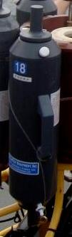
Niskin Bottles Niskin bottles are plastic bottles with lids on both ends which are attached by springs or rubber. When deployed, both lids are held open until the desired sample depth is reached, where the lids are signalled shut simultaneously, therefore containing the water sample from the required depth. Niskin bottles can be used by hand, on a CTD rosette (pictured left) where the bottles are shut by an electronic signal, or attached to a hydroline with clamps where a messenger is sent down to trigger the shutting mechanism. Niskin bottles are simple and relatively reliable, although they can sometimes misfire during sampling. They are also equipped with an air inlet at the top and a water outlet valve at the bottom to slowly bleed out smaller subsamples (the white fixtures in the picture, left).
|
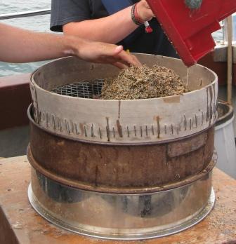 |
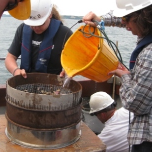
Sieve Stack A very simple geological tool, the sieve stack is used to separate out raw sediment samples into subsamples by grain diameter. The largest mesh size is at the top of the stack, and they become progressively smaller down the stack. A very rudimentary stack was used with 3 sieves of mesh sizes 10mm, 2mm and 1mm.
|
Light Sensor The light sensor provides information on light penetration at depth. The system consists of two light sensors fitted with opal lenses to act as Lambertian surfaces. These remove directionality of incident light which would otherwise give erroneous results and allow for the readings to be unbiased with respect to its orientation. A sensor is placed in the air above the water surface to measure incident light, while another sensor is placed on a frame and lowered into the water. The underwater sensor is held at a known depth and the light levels both at the surface and depth are recorded. These are then used to calculate the ratio of light reaching different water depths. From these ratios, light attenuation can be calculated.
|
Thermosalinograph A thermosalinograph is an on-board instrument which measures the temperature and conductivity of sea surface waters by making use of pumped water systems. Temperature is measured using a thermistor which is a resistor whose resistance varies with temperature, and conductivity is measured using two electrodes. From this data salinity can also be calculated by using conductivity data and correcting it for temperature and salinity.
|
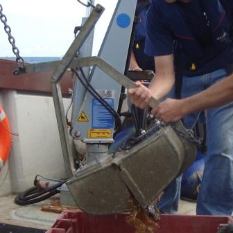 |
Van
Veen Grab The van Veen grab is a simple yet effective device designed to sample sediment and non-mobile biota from the sea floor. Whilst the van Veen grab is not intended to sample motile biota, it is not uncommon to pick up these organisms when sampling, especially if the organisms are normally associated with the sediment. The van Veen grab is best suited to sampling in soft to medium unconsolidated bottom sediments. Models may be equipped with additional weights to improve sediment penetration, or viewing hatches to allow inspection of the sample prior to opening the jaws. The grab is armed and lowered via a winch to the sea floor. Upon contact with the bottom tension is removed from the arming mechanism, causing it to trigger. Upon raising the grab, the two lever arms are pulled together, causing the jaws to close and trap the sample.
|
 |
Video Tow Camera This is a camera attached to a frame which is dragged slowly behind the Xplorer near to the sea bed. The camera records a video feed which is viewed real time with an on-board monitor. The frame is fitted with a red plastic fin which helps to keep the camera at a fixed orientation relative to the direction of tow. A good indication of the nature of the benthic habitat can be obtained from studying the video and noting down the biology and geology observed. This is useful because it may be used in concert with a van Veen grab sampler to obtain an idea of the nature of the sea bed to determine whether or not a grab sample of the area is possible or useful.
|
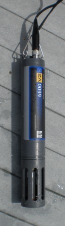 |
YSI
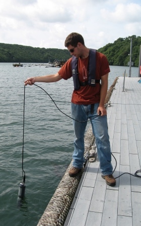
Probe YSI’s 6600 V2 Probe is a handheld multi-probe used to measure temperature, salinity, turbidity, chlorophyll, depth and dissolved oxygen. It is small and lightweight, and so is deployed by lowering it into the water by hand. The probe’s outputs can be monitored in real time when connected to a computer.
|
|
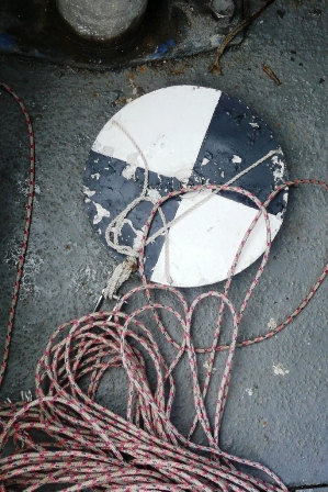
Secchi disk The Secchi disk is a simple but proven device used to determine turbidity. It is a metal disc painted black and white in alternating quadrants. The disk is lowered by an observer until it is no longer visible, and then raised again until it is just visible again. This depth is measured by recording the length of the line deployed and is known as the Secchi depth.
|
R. V Callista
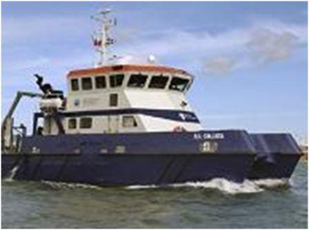
R. V. Callista is the largest vessel belonging to the National Oceanography centre and is purpose built for research. The large rear working deck area and A frame that has a lifting capacity of 4 tonnes for equipment deployment allows it to be used both for research and commissioned work on the South coast. R.V. Callista is 19.75 meters long with a twin hull.
Length overall: 19.75m
Breadth: 7.40m
Depth midship: 2.85m
Speed: 15Kts
Maximum passengers: 30
A-frame: 4 tonne
Bill Conway
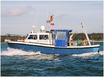
Length Overall: 11.74m
Breadth: 3.96m
Depth midship: 1.3m
Speed: 10Kts
Maximum passengers: 1 Crew: 1 Scientists:12
A-Frame: 750Kg
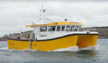 S. V. Xplorer
The Xplorer is a survey vessel, specialized for dive support research. The working deck area at the rear of the vessel enables equipment to be deployed by a crane (1 tonne capacity) allowing bathymetric and geophysical surveying to be carried out. Stations can be sampled quickly as the Xplorer is a reasonably fast vessel (25 Knots) it is also an extremely manoeuvrable vessel capable of going both inshore and offshore and is therefore great for estuarine work.
Length Overall: 11.88m
Breadth: 5.2m
Depth midship: 1.2m
Speed: 25 knots
Offshore Boat Work Procedures
Date:
28/06/10 Tides: LW 12:54 HW 18:26 (All times GMT). Weather: No cloud
cover, light breeze
Objective: Sample ocean chemistry, biology, and physics to determine
the location of the offshore seasonal thermocline.
 |
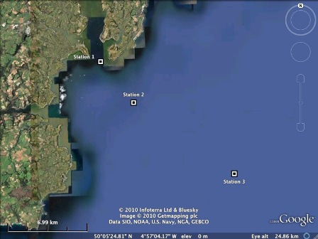
Station 1: Blackrock 50°08.327N, 005°01.580W. Arrived 11:33.
Departed 12:30. Transect between Stations 1 and 2 was recorded on the ADCP. Travel was perpendicular to the coast, and ADCP was monitored until zooplankton were visible as backscatter at Station 2. |
||
|
Station
2: Offshore front 50°06.278N, 004°58.996W. Arrived 12:43. Departed
14:11. |
 |
||
 |
Station 3: Offshore (8.3nm from Blackrock)
50°02.823N, 004°51.411W. Arrived 14:41. ADCP start was delayed due to malfunctioning, but picked up soon after arriving. CDT: Lowered to 62.7 meters. Niskin bottles fired at 62.4, 41.5, 27.1, and 3.5 meters. Samples were separated and filtered for analysis of dissolved oxygen, silicon, nutrients, chlorophyll, and phytoplankton. Vertical plankton nets: Two samples were collected from different depths (40-20m, and 20m-surface) Samples were placed into large bottles for lab analysis. Secchi disk: Depth was found to be 10 meters. |
||
 Wet
Lab on RV Callista
Wet
Lab on RV Callista
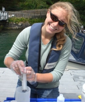
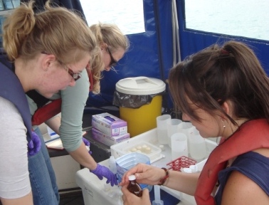
The water samples taken from Niskin bottles where used to analysis Nitrate, Phosphate and Silicon. From each Niskin bottle 100ml of the sample was measured using a 50ml syringe and filtered using a glass fibre filter. This was placed into a medicine bottle and used for Nitrate and Phosphate analysis. From the same Niskin bottle, 50ml of the sample was again measured and filtered into a 50ml plastic bottle and used for Silicon analysis. These bottles were then placed into the fridge.
Results
 |
 |
 |
 |
 |
|
Station 1 CTD Data Click to Enlarge |
Station 2 CTD Data Click to Enlarge |
Station 3 CTD Data Click to Enlarge |
Station 2 Nutrient Samples Click to Enlarge |
Station 3 Nutrient Samples Click to Enlarge |
 |
 |
 |
|
Station 1 ADCP Data Click to Enlarge |
Station 2 ADCP Data Click to Enlarge |
Station 3 ADCP Data Click to Enlarge |
|
|
|
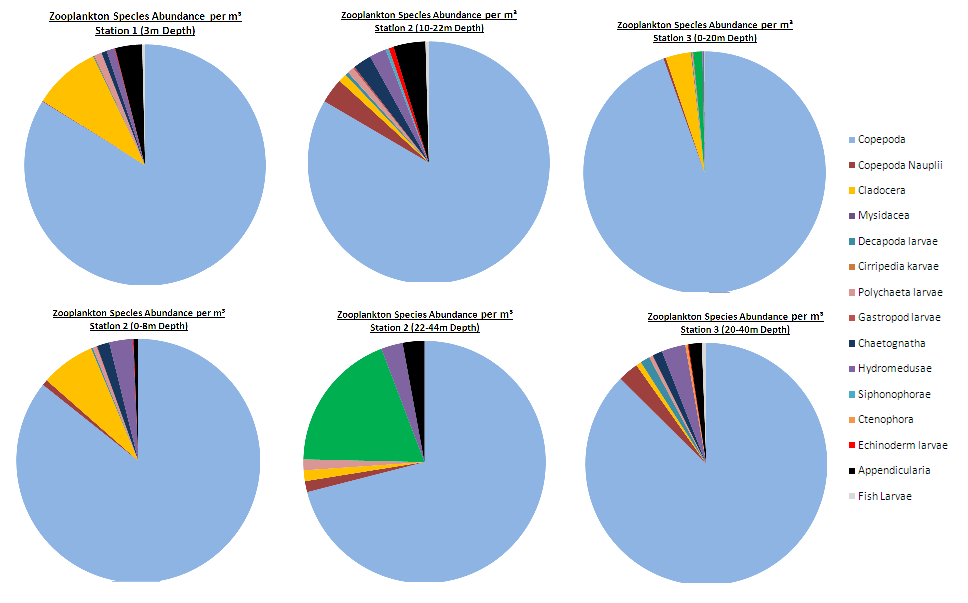
Zooplankton
Abundances from Offshore Net Samples |
Analysis
STATION 1
ADCP data for flow direction shows a general south or southeasterly flow at station 1 , and the velocity of this flow tends to decrease with depth. Data collection at station 1 was carried out during the ebb tide and station 1 is located near Black Rock, which is in the Fal estuary, so the ADCP data shown reflects what would be expected to be seen under such conditions in this location. The temperature profile shows barely any temperature change with a decrease of only 0.3°C from the surface to a depth of 15 metres. Chlorophyll levels increase slightly with depth but do not exceed a concentration of 0.8µg/L at any point in the water column. Together the ADCP and CTD data indicate that the water column was well mixed in this area, which may be due to the shallow depths usually around 17m which means that the wind mixing is able to mix the entire water column.
Zooplankton samples show copepods as the dominate water column resident. In Station 1 at 3m depth the next largest populations were Cladocera, and Appendicularia. Also, very little phytoplankton was found possibly due to copepod grazing.
STATION 2
Station 2 was selected due to a clear layer of increased backscatter in the ADCP data at around 5 to 12 metres’ depth, caused by an above average density of zooplankton. This was a clue that the water column would have stratification due to a thermocline. The CTD profiles confirmed that there was stratification at this location; a clear thermocline can be seen at 5 to 8 metres depth, with a warmer upper layer at 15.5°C and an underlying layer up to 3.5°C cooler. Looking at previous research based on data from the L4 station nearby it is probable that the stratification observed is seasonal and linked to a tidal front which is in the Western Channel (Pingree and Griffiths, 1978). The chlorophyll profile shows a peak of 1.25µg/L at about 16m at the bottom of the thermocline compared to 0.3µg/L at the surface, which is because this is the optimum depth for the phytoplankton, allowing them to benefit from maximum light levels while remaining in the nutrient rich bottom layer. Nitrate and silicon have a minima at the chlorophyll maximum, due to depletion by phytoplankton growth.
The average flow direction and magnitude through the water column is constant in a south west direction, however when studied in more detail, the direction of flow slowly changes with depth from westward flow at the surface and rotates in an anticlockwise direction down to a southeast directed current close to the seafloor. There is an increase in turbidity and flow velocity at the seafloor which illustrates the friction between flow at the base of the water column and the seabed.
The increased layer of backscatter which is caused by zooplankton in the ADCP data for this station shows internal waves occuring in this region. This is seen at a depth from about 5 to 9 metres, which coincides with the depth of the thermocline at this site. The ADCP data for flow velocity also shows an increased velocity magnitude at the same depth which further supports the existence of internal waves. These internal waves may have been caused at the interface between the warmer upper layer of water and the cooler underlying layer by the change in topography at the shelf break due to strong winds over the North Atlantic. Alternatively the internal waves may have been a result of strong tides, which is a possibility considering the data for this station was collected just after the ebb tide of a spring tide.
Zooplankton collected by vertical net at depth between 0-8m, 10-22m, and 22-44m. Again copepods dominate the profile. However, Cladocera were present in greater abundance in shallower waters than in the deeper water samples. In the deepest sample, 22-44m, Siphonophorae gained abundance in comparison to other samples. Again no phytoplankton was identified.
STATION 3
CTD data for station 3 indicates that this station has a stronger thermocline than station 2, with a drop of 6°C over a depth of less than 15 metres. The temperature profile shows a main thermocline to a depth of 18m, but there is also evidence of a secondary thermocline which reaches a deeper depth of 37 metres before the bottom homogenous layer is reached. When heating of the surface waters occurs in spring and summer months, it is mixed down to create the mixed upper layer by wind mixing. Deeper thermoclines can be caused by periods of higher wind mixing such as a storm which increase the depth of the mixed layer. As these are not usual conditions, a thermocline of normal depth will develop again above this with further heating of surface waters. As observed for station 2, there is a chlorophyll maximum under the main thermocline however this is seen on a much greater level, with concentration surpassing 6.5µg/L at the peak compared to 1.25µg/L for station 2. The CTD data for chlorophyll gave significantly different data for the chlorophyll peak on the drop and on the return, suggesting that the chlorophyll distribution is very patchy. ADCP data shows two layers of increased backscatter which correspond to depths both above and below the chlorophyll peak, suggesting that zooplankton may be gazing the phytoplankton from above and below.
The upper layer above the thermocline shows flows in a northwest direction, while the bottom layer is moving in a southeast direction. This indicates that there will be shear flow between the layers moving in opposite directions at a depth of 37 metres. Flow magnitude illustrates that above the main thermocline flow travels 3 times as fast as the flow below, so there will also be shear along the main thermocline, even though both water bodies are moving in the same direction.
Zooplankton samples were taken from 0-20m and 20-40m. Copepods most represented in the this offshore sample. In the shallower depths Cladocera and Siphinophorae were found. In the deeper samples copepod nauplii and Hydromedusae were present in greater abundance that in shallower samples. As with other stations phytoplankton counts were very low.
Date: 30/06.2010 Tides: LW
14:01 HW 19:30 (All
times GMT). Weather: Partly cloudy slight wind
Objective: of the day while
out on the explorer was to determine the different benthic areas through habitat
mapping and monitoring.
To get an idea of the seabed a sidescan sonar was ran that helped to determine where the grab samples would be taken. Before deploying the van Veen grab, video footage of the sea bed was captured and areas likely to yield interesting grab samples were noted. These were returned to and sampled. The grab was rigged up to the Xplorer’s crane, set open and dropped to the sea bed. This was then retrieved and brought aboard, photographed through the viewing window with position and time data before being opened into a large bin. The sample was then examined by hand by all the group and organisms identified as thoroughly as possible with the aid of an identification book. One sample from Station 4 had large amounts of sediment, which were sorted with the sieve stack (mesh sizes 10mm, 2mm & 1mm) and each sieve examined separately.
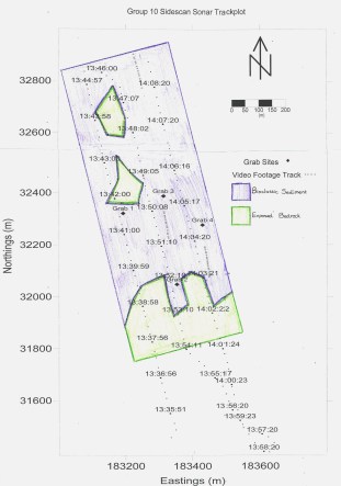
Sidescan Sonar
|
Line 5: Heading of 347°
Line 6: Heading of 165°
Line 7: Heading of 345° |
|
|
|
Sidescan sonar imagery overlaid with interpretive habitat map. Green is exposed bedrock, and purple is bioclastic sediments Click image to enlarge. |
Interpretive habitat map plotted over the shiptrack of the SV Xplorer. Click image to enlarge. |
Grab Sample Observations
| Location | Time GMT | Biology | Bedding | Observations |
|---|---|---|---|---|
|
50°09.0574'N
005°02.1715'W |
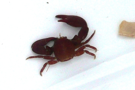
14:47:45 | Tube worms, sea belt, tiny gastropods, sea squirts, razor clam, crab, shrimp, rhodophyta, brittle star (Corella paralellogramma), hermit crab | Poorly sorted, angular, 1-30mm biolclastics. Kelp anchored to sub-angular, foliated tan-brown metamorphic rock | |
|
50°08.9198'N
005°02.0339W |
15:09:18 | Sea belt | Sediment, rock | |
|
50°09.1054'N
005°02.0806'W |
15:22:24 | Sea belt, crab, gastropods, isopods, Cirolanida, bryozoa, slit limpets, polyplacophora | Rocks | Rocks kept grab open so smaller bits fell out |
|
50°09.0462'N
005°01.9777'W |
15:56:03 | Rhodophyca, heart urchin, bivalves, flatworm, fish larva? | Coarse sand, rocks, broken shell/bioclastics | Seived sample in 1cm, 2mm, 1mm stack |
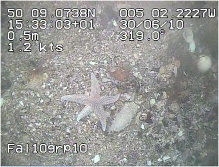
Video Observations
| Line # | Location | Timestamp GMT | Biology | Bedding |
|---|---|---|---|---|
| 6 |
50°09.0652'N
005°02 .2061'W |
14:32:18 | Kelp, starfish | Broken Shells-Coarse |
| 6 |
50°09.0739'N
005°02.2230'W |
14:33:04 | Starfish | Broken Shells-Coarse |
| 6 |
50°09
.0802'N 005°02.2330'W |
14:33:46 | Rhodophyca | Broken Shells-Coarse |
| 6 |
50°09.1021'N
005°02.2476'W |
14:35:47 | Kelp | Getting rockier- big rocks slate? |
| 5 |
50°09.0315'N
005°02.0653'W |
15:16:12 | Kelp | Broken Shells-Coarse |
| 5 |
50°09.0350'N
005°02.0657'W |
15:16:25 | Rhodophyca, Kelp | Broken Shells-Coarse |
| 5 |
50°09.0423'N
005°02.0673'W |
15:16:50 | Starfish | Broken Shells-Coarse |
| 5 |
50°09.0506'N
005°02.0506'W |
15:17:20 | Kelp | Increasing shells |
| 7 |
50°08.9436'N
005°01.9541'W |
15:47:32 | Rhodophyca, Kelp, | Maerl, broken shells, pebbles |
| 7 |
50°08.9600'N
005°01.9577'W |
15:48:59 | Rhodophyca, Kelp, green algae | Maerl, broken shells, pebbles |
| 7 |
50°08.9678'N
005°01.9601'W |
15:49:39 | Starfish, kelp | Maerl, broken shells, pebbles |
| 7 |
50°08.9791'N
005°01.9623'W |
15:50:41 | Starfish, rhodophyca, green algae | Maerl, broken shells, pebbles |
Through the use of sidescan sonar, video recording, and grab samples, we are able to obtain an idea of the marine habitats located in the mouth of the Fal Estuary, particularly in the Blackrock area. Each of these methods has its advantages, but also its limitations. The sidescan sonar printout showed changing substrate, however, the nature of the substrate had to be determined using truthing methods. This problem was solved by using video footage, which indicated areas of bare bedrock, and areas of broken shells and maerl. The video also gave some idea of the biology living in the area, such as starfish and kelp. Grab samples aided in the identification of local biota, although in some areas sampling remained difficult due to the bedrock substrate. Through the use of these grab samples we were able to determine the composition of the seabed and classify particular areas as discrete marine habitats.
Overall, the three techniques used were by themselves insufficient to monitor the condition of marine habitats, but used together, they provide a clear picture of the Blackrock area of Fal Estuary.
|
Date:
02/07/10 Tides: HW 08:34 LW 14:57(All times
GMT). Weather: Partly sunny, light breeze, 4/8 cloud cover. Water samples, YSI profiles and current meter readings were taken from the pontoon located near the King Harry ferry. YSI profiles consisted of readings for dissolved O2 content, turbidity, salinity, temperature, depth and chlorophyll. Profiles were taken at half hourly intervals. A Niskin bottle was used to collect water samples at hourly intervals. A current meter was used to record current direction and velocity at half hour intervals. After, starting at the head of the estuary as far as the tidal state would allow, ADCP transects were taken at 3 locations between Black Rock and Turnaware Point. CTD profiles were also taken at each stations, as well as light readings, Secchi depths and water samples. |
 |
Eulerian Measurements at King Harry's Ferry
 |
King Harry’s Ferry. Arrived 08:55. Departed 12:00. 09:03:10 YSI probe lowered in 1 meter increments to 7 meters depth. At 7m, probe may have touched bottom, causing an increase in turbidity. 09:04:58 Analogue current meter lowered in 1 meter increments to 7 meters depth. At 7m, instrument may have been in seagrass, causing drop in speed. 9:20:12 Two water samples taken (1m and 4m) using a horizontal Niskin bottle. Samples separated and filtered to analyse for nutrients, silicon, and chlorophyll. 09:33:15 YSI probe lowered in 1 meter increments to 7m. At 7m probe may have touched bottom. 09:40:48 Analogue current meter lowered in 1 meter increments to 6 meters depth due to ebb tide. 10:05:29 YSI probe lowered to 4 meters depth. Further readings prevented by arrival of a ferry at the pontoon. 10:13:45 Two water samples taken (1m and 4m) using horizontal Niskin bottle. Samples separated and filtered to analyse for dissolved oxygen, nutrients, silicon, and chlorophyll. 10:16:47 Analogue current meter lowered in 1m increments to 6m depth. 10:31:10 YSI probe lowered to 6 meters depth. Reading at 6m near bottom. 10:48:27 Analogue current meter lowered to 6 meters depth. 10:56:00 Two water samples taken (1m and 4m) using horizontal Niskin bottle. Samples separated and filtered for dissolved oxygen, nutrients, chlorophyll, and silicon. 11:02:17 YSI probe lowered to 6 meters depth. 11:16:48 Analogue current meter lowered to 5 meters depth due to ebb tide. 11:31:31 YSI probe lowered to 5 meters depth. 11:51:00 Analogue current meter lowered to 5 meters depth. 12:00 Remaining four group members were dropped off at the pontoon for the afternoon session on the Conway. Last water samples not taken due to abrupt arrival of Bill Conway at the pontoon. |
 |
Estuary Boat Work Procedures
(All
transects East to West)
|
Station 1: Turnaware Point ADCP transect started 58 meters from shore, ended 37 meters from shore. CDT: 12:45:26. 50°12.135N, 005°02.433W. Lowered to 15 meters. Fired Niskin bottles at 13.61m, 11.95m, 7.97m, 3.94m, and 1.16m. Samples filtered for silicon, nutrients, and chlorophyll. Secchi disk: Depth found to be 2.22 meters Light meter: Lowered to 13 meters , readings taken at 1,2,3,4,5,7,9,11,and 13 meters. |
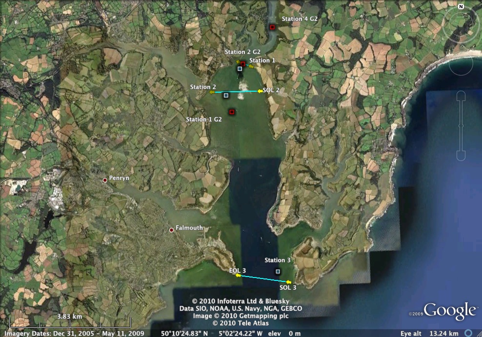 Overview map of sampling locations. Group 2 Station 3 is north of Group 2 Station 4, and just out of view. Click to enlarge. |
|
Station 2: Restronguet Creek ADCP transect started 118 meters from shore (50°11.737N, 005°01.903W), ended 180 meters from shore(50°11.720N, 005°03.190W). CDT: 13:37:00. 50°11.680N, 005°02.801W. Lowered to 15 meters. Fired Niskin bottles at 15.04, 11.46, 7.94, 3.83, and 1.02 meters. Fluorometer failed, showed same values for the entire profile. Samples filtered for silicon, nutrients, chlorophyll, and phytoplankton. Secchi disk: Depth found to be 2.11m Light meter: Lowered to 15 meters, readings taken at 1,2,3,4,5,7,9,11,13, and 15 meters. |
|
|
Station 3: Shag Rock to Pendennis Point ADCP transect started 50m from shore (50°08.471N, 005°01.142W), ended 80m from shore (50°08.588N, 005°02.249W). CDT: 14:53:31. 50°08.667N, 005°01.418W. Lowered to 33 meters. Niskin bottles fired at 25.11, 15.28, 9.93, 5.05, and 1.28 meters. Secchi disk: Depth found to be 3.13m Light meter: Lowered to 15 meters, readings taken at 1,2,3,4,5,7,9,11,13, and 15 meters. |
Wet lab RV Bill Conway
 From each Niskin bottle 50ml of sample was measured
using a measuring cylinder and filtered using a glass fibre filter in to
a medicine bottle, which was used to rinse the bottle. A further 50ml
was measured and filtered through the same filter but this sample was
stored in the bottle and used for Nitrate/ Phosphate analysis. This was
repeated for silicon but the sample was placed into a 50ml plastic
bottle.
From each Niskin bottle 50ml of sample was measured
using a measuring cylinder and filtered using a glass fibre filter in to
a medicine bottle, which was used to rinse the bottle. A further 50ml
was measured and filtered through the same filter but this sample was
stored in the bottle and used for Nitrate/ Phosphate analysis. This was
repeated for silicon but the sample was placed into a 50ml plastic
bottle.
Results
 |
 |
 |
 |
| Transect 1
ADCP Data Click to Enlarge |
Transect 2
ADCP Data Click to Enlarge |
Transect 3
ADCP Data Click to Enlarge |
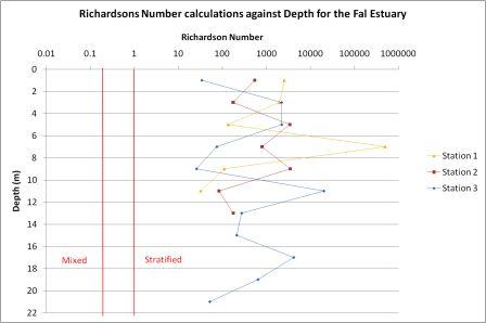
Estuary
Calculated Richardson Numbers Click to Enlarge |
 |
 |
 |
| Station 1
CTD Data Click to Enlarge |
Station 2
CTD Data Click to Enlarge |
Station 3
CTD Data Click to Enlarge |
 |
 |
 |
 |
 |
 |
 |
| Station 1
Nutrient Samples Click to Enlarge |
Station 1,
Group 2 Nutrient Samples Click to Enlarge |
Station 2
Nutrient Samples Click to Enlarge |
Station 2,
Group 2 Nutrient Samples Click to Enlarge |
Station 3
Nutrient Samples Click to Enlarge |
Station 3,
Group 2 Nutrient Samples Click to Enlarge |
Station 4, Group 4 Nutrient
Samples Click to Enlarge |
 |
 |
 |
 |
 |
| Station 2
Phytoplankton Abundance Click to Enlarge |
Station 3
Phytoplankton Abundance Click to Enlarge |
Station 1
Zooplankton Abundance Click to Enlarge |
Station 3
Zooplankton Abundance Click to Enlarge |
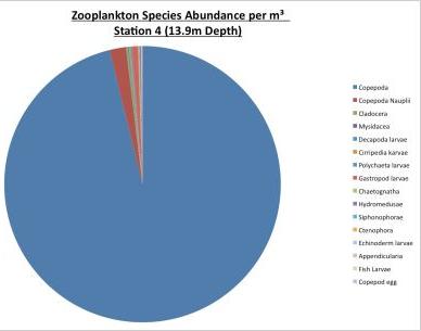
Station 4
Zooplankton Abundance Click to Enlarge |
Analysis
STATION 1
Both stations showed a nutrient peak at 1m (nitrate and phosphate. Station 1 showed a nutrient decrease at 4m corresponding with the chlorophyll maxima. The greatest silicon decrease occurred between the surface and 4m, again coinciding with the chlorophyll maxima.
Station 1’s CTD profile revealed high salinity in the surface layers, peak at 1m. Quite noisy profile, turbidity as defined by transmissometer increases with depth.
The direction of the main flow in the channel is southwards with a small area on the bottom right and in the shallows showing a change in direction to a northwards position. At the time when the transect was recorded there was an ebbing tide which is shown by the southward flowing water mass. The flow magnitude is high on the Western Shore the gets progressively lower towards the shallower eastern shore with a slow velocity also occurring in the bottom right where the direction of flow was changing. The change in both flow direction and magnitude in the bottom right of the plots could be due to the residual circulation that occurs in the Fal estuary due to its large width. In the shallows turbulence occurs due to the friction with the bed again this is shown by the differences in flow direction and magnitude.
The ship stick track indicates that the surface currents are very low near the shallow eastern shore and also travelling in a northward direction which is also shown by the direction of flow plot, getting deeper in the channel the flow reverses to a southward direction and also strengthens this again is representative of the velocity magnitude and flow direction ADCP readings.
The calculated Richardson’s values are all above 1 indicating a stable water column
STATION 1 and 2 (GROUP 2)
Group 2’s data showed almost identical nutrient profiles yet differed greatly with respect to chlorophyll distribution. This may be due to patchy phytoplankton distribution or differing tidal states.
The Station 1 ADCP transect was taken during slack water as the tide was turning, therefore there is very little directionality especially in the surface layers and the flow velocities are also random along the entire transect. The direction is northwards in the bottom of the channel, this could be due to the flooding tide where there are higher salinities due to denser water masses.
The stick plot shows that towards the western shore the surface direction of the flow is non-directional and therefore supports slack water.
The Station 2 data is highly similar to Group 10’s station 1 both in the shape of the bed and the flow direction. However there is little turbulence in the shallow waters , although there is an increase around the bottom of the channel probably caused by the substrate and friction on the bed. The velocity of the flow at this station is lower around the bed due to the friction and turbulence and increases towards the surface where there is lower friction.
The stick plot shows that the surface currents are uniform in both direction and magnitude across the transect , this is not expect as when this is compared to group 10’s station 1 in the shallows the surface flow was small with a faster flow in the channel.
The Richardson number also indicates slack water especially at station 1 when the entire channel is either mixed or in the transition zone between 0.25 and 1. Station 2 is a little more stratified at the surface with more of the points in the transition zone and only 3 points in the mixed zone.
STATION 2
The data generated at station 2 showed a nutrient decrease at 4m, which coincided with the chlorophyll minimum. It is possible that the phytoplankton responsible for depleting the nutrients in the area were themselves grazed by zooplankton. It was also noted that chlorophyll concentration was seen to vary greatly with depth, perhaps indicative of patchy distribution.
Phytoplankton samples were taken at 4m showing high populations of Coscinodiscus (56%). Two equally sized populations (13%)of Guinardia delicautula, Leptocylindrus danicus were found coexisting with the dominant species. Three other species were found at low abundance (6%), these were Alexandrium, Chaetoceros, Thallasiosira.
The direction of the flow is generally southerly although the diagram does show a high change in velocities in shallow waters and to the western edge of the channel, this is highly likely due to turbulence which can occur on short time scales and is common in the Fal estuary. The area of southward flow is also an area of high velocity magnitude at 0.25m/s, this again could be due to the ebbing tide at the surface. It may also relate to an input of fresher water from a tributary which again could increase the flow velocity. As at station 1 the shallow regions indicate turbulence due to non-directional flows with lower velocities. To the western edge of the magnitude profile there is a decreased flow velocity. This may be due to coriolis which acts to the west on an ebbing tide, also the transect length is 1.5km which may to wide enough to allow coriolis to have an effect on the water flow. The substrate may also affect the area for example outcropping rock forms, which may not be shown on the ADCP, would cause turbulence.
The stick track shows the surface turbulence occurring on the western shore due to random flow directions. The surface flow is also stronger in the deep channel, this again correlates with the velocity magnitude profile.
The calculated Richardson’s values are all above 1 indicating a stable water column.
STATION 3 (BLACK ROCK)
A nutrient decrease between 5 and 10m was noted, coinciding with the chlorophyll maxima and silicon maxima. A strong O2 minimum was observed at 8 meters. This may be due to a high presence of copepods grazing on the phytoplankton bloom area. An intermediate temperature layer was present between 5 and 9 meters of 14.5°C . This layer coincided with a chlorophyll maximum.
The CTD profile showed a more defined thermocline. A turbidity increase was noted between 5 and 8 meters. This coincides with the O2 minimum and suspected copepod maximum.
At 10m phytoplankton was sampled near Black Rock at the mouth of the estuary. Again the dominant species was Coscinodiscus (44%), followed by Guinardia delicatula (17%), and Guinardia flaccida (11%). Also present, but less abundant were Leptocylindrus danicus (6%), Thalassiosira (6%), Thalassiosira ratula (6%), Karinia mikimotoi (5%) and Chaetoceros (5%).
This transect was done just before the tide turned to a flooding tide. The flow velocities are generally small with a section at the surface in the middle of the transect have a relatively strong current with a southwardly direction. This could be due to an ebb tide underlying a strong flood tide, especially as the tide is turning as they can both be present. The slower velocities correlate with a northward flow direction deflected to the western shore, again this may be due to coriolis as the transect is 1.6km in length. On the eastern shore rocky substrate is shown by the ADCP, this was verified by the geophysics data produced, this produced turbulence in this area due to friction and therefore the flow velocities are low and non-directional.
The effects of Black Rock on currents can clearly be seen on the ADCP data for transect 3. It can be seen by a decrease in surface velocity at about 1000m from the beginning of the transect in the east, with an increased southward current on either side due to the build up of ebbing water on either side and interactions with the bottom bedrock. Black Rock is also shown in the velocity plot by an increase in turbulence in the area again due to the friction with the bedrocks. The stick plot also indicates Black Rock in the same location by very little surface flow due to the ‘shadow zone’ it creates as water masses are deflected around it. Southward surface flows of a small velocity are also shown on either side of Black Rock.
The calculated Richardson’s values are all above 1 indicating a stable water column.
STATION 1 (GROUP 2)
Spikes in silicon were noted all through the profile, perhaps due unusual mixing from boat traffic.
Zooplankton was sampled at 11m depth by vertical net, carried out by group 2. By far the most common organisms were Copepods and nauplii.
STATION 3 (GROUP 2)
All measured properties showed a decrease in concentration with depth, with the exception of phosphate. Trends are difficult to identify in great detail as only 2 samples were collected for this station.
At the head of the estuary zooplankton was sampled at 6.7m. Copepods (76%) and copepod nauplii (7%)were the dominant organism found. Other species were found at far lower abundances including Ctenophora (2%), Siphenophorae (2%), and Hydromedusae (2%).
STATION 4 (GROUP 2)
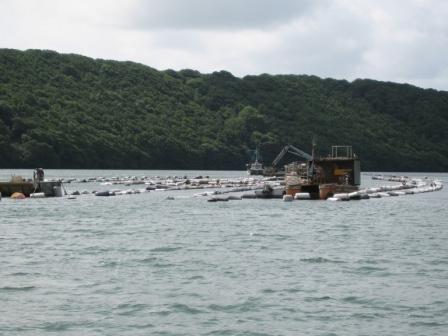
This site was situated close to a mussel farm. Chlorophyll showed little change with depth. Surface concentration of nitrate and phosphate are higher than at other stations, perhaps due to the presence of the mussel farms.
Copepods dominated the collection from 13.9m at station 4. Other abundance counts were so low as to be negligible.
Lab Analysis for Offshore and Estuary
Chemical
analysis procedure
Nutrient chemical analysis
Nitrate, phosphate, silicate, chlorophyll,
and dissolved oxygen samples were gathered using niskin bottles on a CTD
rosette. Using flow injection procedurally by Johnson and Petty (1983)
nitrate samples were analyzed for concentration with some
modification. Phosphate, silicate, and chlorophyll samples were
analyzed using methods of Parson (1984) with spectrometry. Dissolved
oxygen was analyzed using the Winkler method of titration as given by
Grasshoff (1999) to find concentrations in the different samples.
During lab analysis for estuary samples, slight modifications were made
to the procedure for silicon analysis. Two riverine samples (500
and 550) were diluted by a factor of two to bring them down to a
readable absorption, and a separate set of standards were made up to
compare to these two samples.
Biological analysis procedure
Zooplankton
Samples were taken at three stations
offshore using bongo nets (station 1) and vertical plankton nets
(station 2 and 3). The net mesh of both nets was 200 microns with a
diameter of 60 cm. Samples were stored in plastic jugs and labeled
in terms of depth and location of collection. On board RV Callista
formalin was added to the sample. In the lab the following day samples
were analyzed using buggeroff counting chamber with 5 ml of sample, 4
replicates for each sample, and dissecting microscope. Chambers allowed
easy identification and counting. Coastal Plankton by Larkink
and Westheide (2006) aided in identification. Counts were then used to
calculate the total amount of species collected.
Phytoplankton
Phytoplankton samples were taken from
Niskin bottles at the different sites of collection. 100ml of sample
were added to a lugols solution in brown glass bottles and then stored
on ice. The following day in the lab samples were counted per 1 ml of
liquid with a single replicate. Sample counts were carried out on
gridded slides and microscope at 4 and 10 times magnification.
Dissolved Oxygen Analysis
The Winkler method was used to analysis the % saturation of dissolved oxygen in a sample. When the samples where collected for dissolved oxygen analysis glass containers were filled directly from the Niskin bottles to be sure that little contact with the open atmosphere occurred. Alkaline Iodide and Manganese Chloride were then added to the sample and agitated before storing submerged in cool water. When in the laboratory the sample bottles had 1ml of sulphuric acid added and then an auto stirring magnet was used to keep the sample mixed. The solution was then titrated with sodium thiosulphate (normality of 0.22) using an auto-burette. The end point of the titration …
Chlorophyll Concentration Analysis
Chlorophyll concentrations were determined by filtering 100ml of seawater from the Niskin bottle samples through glass fibre filters to obtain chlorophyll samples. Samples were put into 6ml of acetone and left in a fridge overnight. This breaks up the cells so that the chlorophyll is released into solution in the acetone. The acetone samples were processed in the laboratory the next day. A fluorometer was used which measured the amount of reflection off the suspended chlorophyll particles in the acetone solution samples. The fluorometer readings were recorded and then acetone corrected to get the actual chlorophyll concentration in the sample.
Over the last week we analyzed the Fal estuary from a chemical, biological, and physical perspective. The data show a well-mixed estuary and thermally-stratified coastal sea dominated by zooplankton grazers, especially copepods. Nutrient levels remain high due to terrestrial anthropogenic inputs. The estuary mixing is tide-dominated. A strong thermocline has developed approximately 6 nautical miles from the mouth of the estuary, and the coastal sea waters are extremely stable.
Articles:
Bryan, G.W. and Langston, W. J. 1992, ‘Bioavailability, accumulation and effects of heavy metals in sediments with special reference to United Kingdom estuaries – a review. Environmental Pollution’, 76. 89-131.
Farnham, W.F. and Bishop, G. M. 1985, ‘Survey of the Fal Estuary, Cornwall’, 10. 53-63.
Johnson, K. S. and Petty, R. L. 1983, ‘Determination of nitrate and vitrite in seawater by flow injection analysis’, American Society of Limnology and Oceanography 28, 6, 1260-1266.
Larkink, O. and Westheide, W. 2006, 'Coastal plankton: Photo guide for European Seas' in Verlag Dr. Friedrich Pfeil, Munchen.
Pingree, R.D. and Griffiths D.K., 1978, ‘Tidal Fronts on the Shelf Seas Around the British Isles’, Journal of Geophysical Research, 83, 4615-4622.
Websites:
National Oceanography research vessels, [Online], Available: http://www.soes.soton.ac.uk/resources/boats/vessels.html [accessed 2010,July 2nd].
Nansen closing net image, [Online], Available : http://www.hydrobios.de/englisch/produkte_netze_vertikal.html [accessed 2010, July 4th].
Van veen grab image, [Online], Available: http://www.aims.gov.au/pages/reflib/bigbank/images/vanveen-480.gif [accessed 2010, July 2nd].
Valeport Current meter image , [Online], Available: http://www.valeport.co.uk/Products/CurrentMeters.aspx [accessed 2010, July 2nd].
Fal estuary location and physical description, [Online], Available: http://projects.exeter.ac.uk/geomincentre/estuary/Main/loc.htm [accessed 2010, July 1st].
Fal estuary special area of conservation, [Online], Available: http://www.cornwall.gov.uk/default.aspx?page=13694 [accessed 2010, July 1st].
We would like to thank the boats crews, lab technicians, lecturers and the Falmouth Marine School. The views and opinions expressed in this site are those of the individuals in the group and do not necessarily represent the views of Southampton University or the National Oceanography Centre.