
TOP
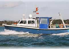
VESSELS
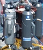
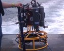
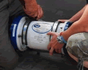
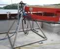
EQUIPMENT
LABORATORY
OFFSHORE
Physical
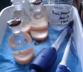
Chemical
Biological
Summary
GEOPHYSICS
Scans & Video
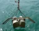
Grabs
Summary
TOP
VESSELS
EQUIPMENT
LABORATORY
OFFSHORE
Physical
Chemical
Biological
Summary
GEOPHYSICS
Scans & Video
Grabs
Summary
 |
 |
|||||||||||||||||||||||||||||||||||||||||||||||||||||||||||||||||||||||||||||||||||||||||||||||||||||||||||||||||||||||||||||||||||||||||||||||||||||||||||||||||||||||||||||||||||||||||||||||||||||||||||||||||||||||||||||||||||||||||||||||||
INTRODUCTIONPlease scroll slightly horizontally to make vertical scrollbar visible
DOWNLOAD LOGBOOK Typed Word Document. (.doc file) DOWNLOAD GOOGLE EARTH FILE Shows all station detail of all boat practicals. (.kmz file) Welcome to the website of Group 1 for the Falmouth fieldcourse. Falmouth is located on the southern coast of Cornwall in the south west of the UK. The town is located on the Fal estuary which is a ria that is recognised as being the first port from the west Atlantic and also a special area of conservation (SAC) due to the maerl and sea grass beds found in the area. Although there are several rivers that flow into the Fal, the estuary is principally tidally dominated. The course took place from Monday 28th June 2010 to Friday 9th July 2010. Here you will find complete documentation of the course. Group 1 consists of eleven oceanography and marine biology students from the University of Southampton. The aim of the course was to apply the skills and knowledge aquired through the degree programmes and throughly analsyse the data obtained. |
Timetable
Throughout the website, photos and graphs can be enlarged by mouse over All tides are Falmouth unless otherwise stated. All photos are taken by the students unless otherwise stated. |
|||||||||||||||||||||||||||||||||||||||||||||||||||||||||||||||||||||||||||||||||||||||||||||||||||||||||||||||||||||||||||||||||||||||||||||||||||||||||||||||||||||||||||||||||||||||||||||||||||||||||||||||||||||||||||||||||||||||||||||||||
VESSELS
|
||||||||||||||||||||||||||||||||||||||||||||||||||||||||||||||||||||||||||||||||||||||||||||||||||||||||||||||||||||||||||||||||||||||||||||||||||||||||||||||||||||||||||||||||||||||||||||||||||||||||||||||||||||||||||||||||||||||||||||||||||
EQUIPMENT
|
||||||||||||||||||||||||||||||||||||||||||||||||||||||||||||||||||||||||||||||||||||||||||||||||||||||||||||||||||||||||||||||||||||||||||||||||||||||||||||||||||||||||||||||||||||||||||||||||||||||||||||||||||||||||||||||||||||||||||||||||||
LAB TECHNIQUES
|
||||||||||||||||||||||||||||||||||||||||||||||||||||||||||||||||||||||||||||||||||||||||||||||||||||||||||||||||||||||||||||||||||||||||||||||||||||||||||||||||||||||||||||||||||||||||||||||||||||||||||||||||||||||||||||||||||||||||||||||||||
OFFSHORE Boat practical
|
||||||||||||||||||||||||||||||||||||||||||||||||||||||||||||||||||||||||||||||||||||||||||||||||||||||||||||||||||||||||||||||||||||||||||||||||||||||||||||||||||||||||||||||||||||||||||||||||||||||||||||||||||||||||||||||||||||||||||||||||||
|
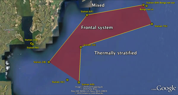
Introduction to Offshore Practical The aim of the offshore cruise was to attempt to map the extent of the front offshore of Falmouth. Tidal mixed fronts are characterised by horizontal gradients in temperature and salinity. Fronts are often sites of high biomass, particularly phytoplankton and related zooplankton populations. The position of a tidally mixed front is determined by the interaction of surface heating and tidal mixing.Away from the influence of major sources of fresh water, in the summer months, temperate shelf seas are separated into thermally stratified and well mixed regions (Sharples & Simpson, 2009). In order to determine the extent of the front, it was necessary to obtain the physical characteristics of the water column to aid in identifying the mixed side and the stratified side. Such a division is noticeably visible in CTD profiles and ADCP backscatter images.
Offshore, during periods of increased insolation, shelf seas can exhibit a horizontal thermal gradient, where deeper water columns that are not influenced by tidal mixing become thermally stratified compared to the tidally mixed water in shallower areas. This is physically represented as a horizontal gradient in temperature (and possibly salinity) and is known as a tidal mixing front. These physical gradients are normally accompanied by similar rapid changes in chemical and biological features. Fronts are therefore important oceanographic features with defining physical, chemical and biological characteristics. The mixed side of a front can be identified by physical and chemical parameters that do not vary to any great extent vertically in the water column. However on the stratified side, the development of a vertical thermocline that results from insolation and the reduced influence of tidal mixing produces more pronounced changes in the same physical and chemical parameters through the water column. On the mixed side of the front it would be expected that primary productivity is limited. Phytoplankton require a certain light level in order to photosynthesize efficiently and thus mixing will limit how long they can remain in the euphotic zone. However, provided the critical depth remains below the mixed depth, net positive photosynthesis is still possible. As the water becomes thermally stratified, any nutrients above the thermocline may be rapidly utilized by primary producers resulting in a nutrient depleted upper layer and increased nutrient concentration in the lower layer due to remineralisation. This would also normally be associated with depleted oxygen concentration in the lower layer. By looking at these parameters in totality, it may be possible to identify the extremes of either side of the front and thus chart its extent. |

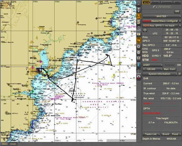
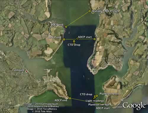
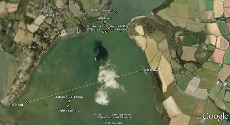
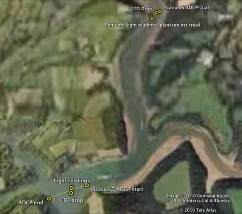
Fig.
5. Track data of Offshore trip. |
|||||||||||||||||||||||||||||||||||||||||||||||||||||||||||||||||||||||||||||||||||||||||||||||||||||||||||
|
||||||||||||||||||||||||||||||||||||||||||||||||||||||||||||||||||||||||||||||||||||||||||||||||||||||||||||
|
||||||||||||||||||||||||||||||||||||||||||||||||||||||||||||||||||||||||||||||||||||||||||||||||||||||||||||
|
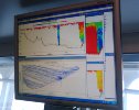
Physical Results
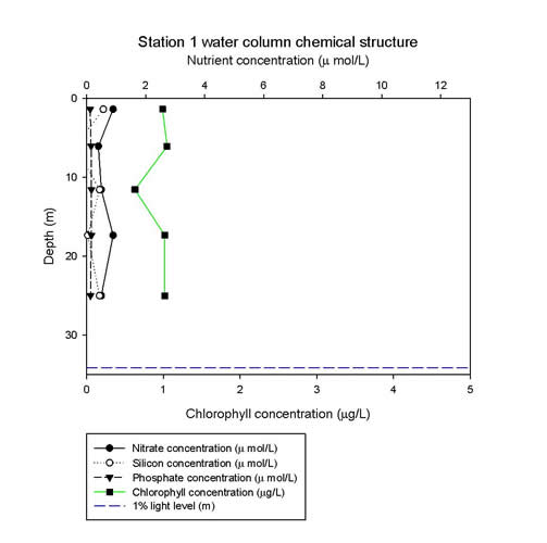
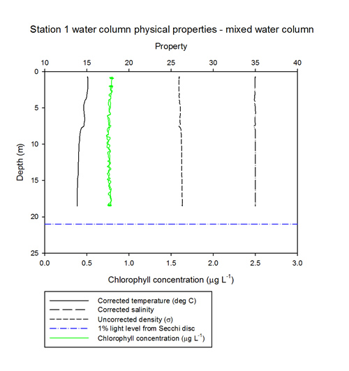
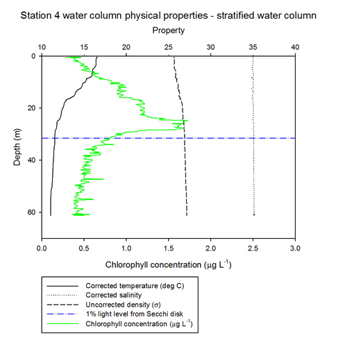
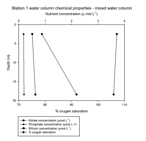
Offshore from Falmouth Mouse over graphs to enlarge on page. The CTD was an important tool for finding frontal systems relatively quickly, overall there were nine CTD stations and using these data the frontal system was shown to run parallel to the coastline. The depth of the Chlorophyll maximum could be estimated by using values from the CTD system. Parameters such as light intensity and density could be seen throughout depth, these helped to explain the reasons for chemical and biological characteristics seen at the site.
Generally, stations on the mixed side of
the front showed homogeneous
characteristics with depth. Temperature
and salinity followed straight,
near-vertical lines on the plots of
stations 1, 2, 5, 6 and 9, suggesting a
mixed system. Mixing was the result of
tidal currents generating shear stress
with the seabed, and wind shear stress
at the surface. In shallower waters,
these two mixed cells meet, and the
entire water column becomes mixed; the
mixed side of the front is therefore
always the shallower side. Recorded
temeperatures were around 15 degrees
celsius for the mixed water column. In
terms of light and chlorophyll, station
1 showed uniform distribution of
chlorophyll with depth, at 0.75µg/L. The
1% light level was 21m (see station 1
plot, figure 7) |
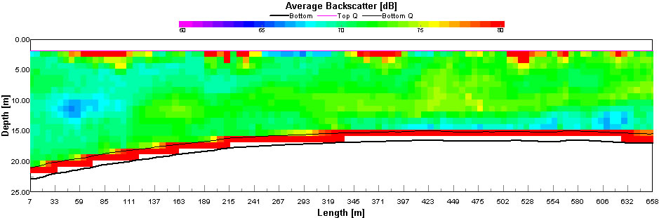
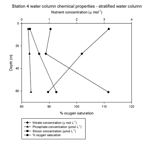
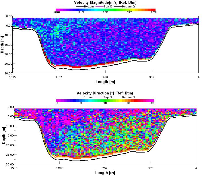
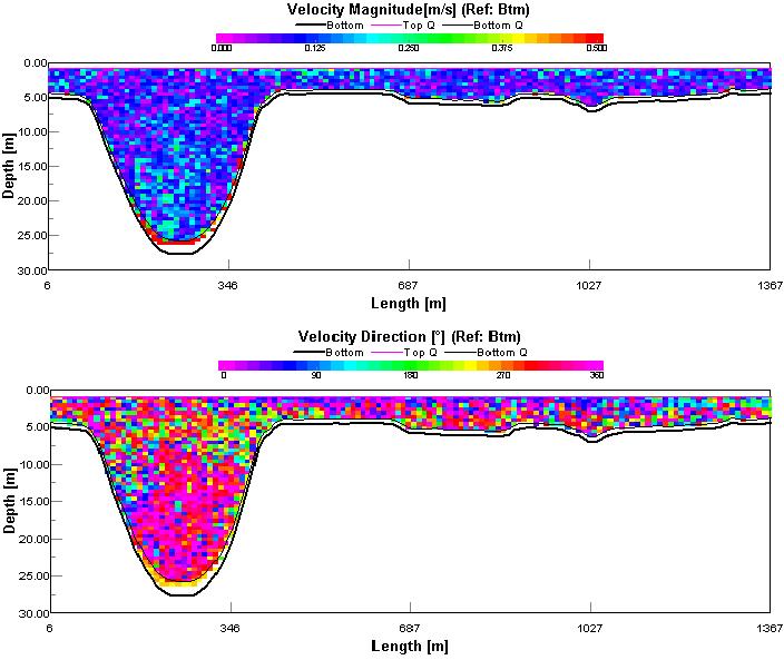
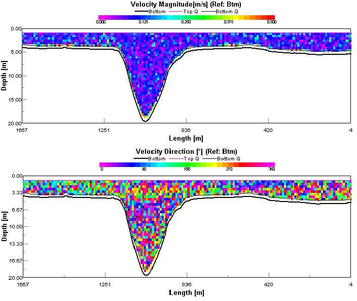
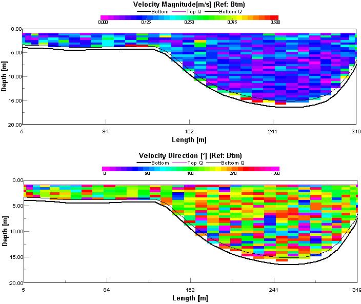
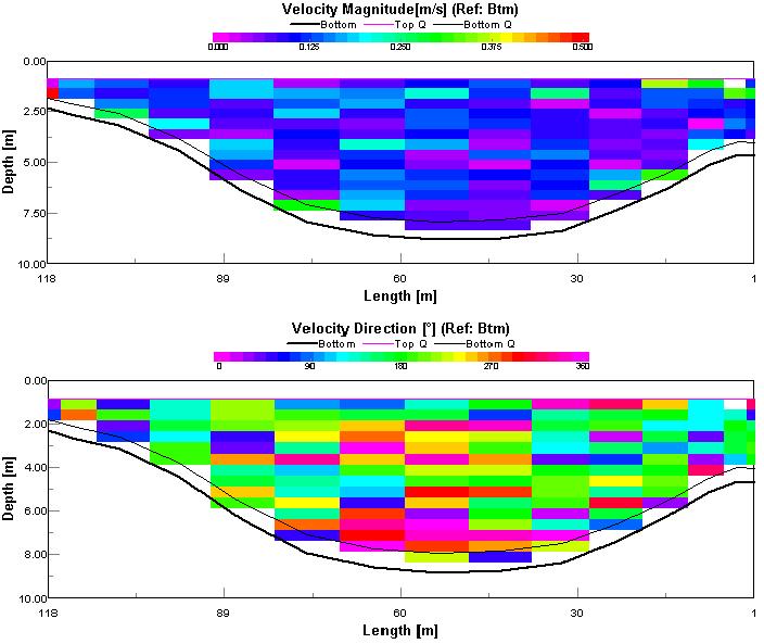
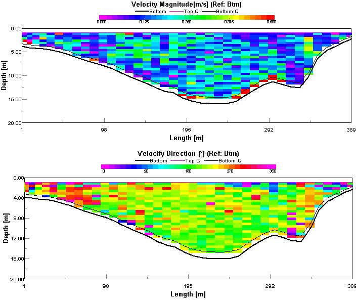
ADCP & Richardson Number (Mouse over images to enlarge) Utilising the current velocity data from the ADCP the Richardson Number could be calculated. The Richardson Number (Ri) is the ratio of stratification to the square of shear in horizontal current. A Ri below 0.25 is indicative of mixing, a Ri value above 1 suggests stratification, and a Ri value between 0.25 and 1 indicates transition between a state of mixing and stratification. Station 1 (Mixed region) For station 1 the Richardson Number was calculated to be 0.094, which is well below the critical value of 0.25 and so it suggests a well mixed region. This is also presented by the backscatter image. Station 2 (Stratified region) 
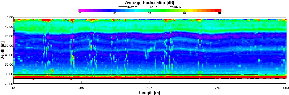
For station 4 the Richardson Number was calculated to be 1.430, which is well above the critical value of 1 and so it is indicative of strong stratification in this region. This is also presented by the backscatter image. |
|||||||||||||||||||||||||||||||||||||||||||||||||||||||||||||||||||||||||||||||||||||||||||||||||||||||||||
Chemical Results
Offshore from Falmouth
|
||||||||||||||||||||||||||||||||||||||||||||||||||||||||||||||||||||||||||||||||||||||||||||||||||||||||||||
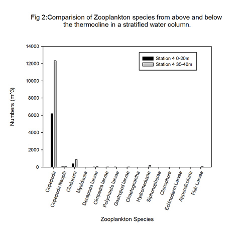
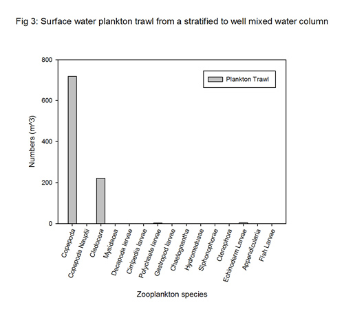
Biological
Results Offshore from Falmouth
|
||||||||||||||||||||||||||||||||||||||||||||||||||||||||||||||||||||||||||||||||||||||||||||||||||||||||||||
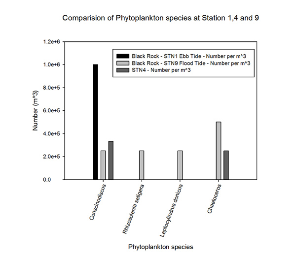
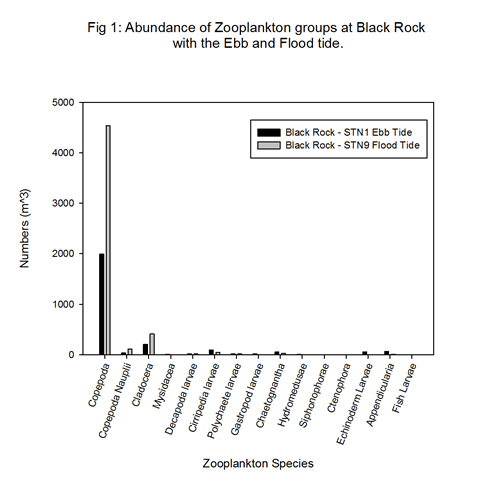
Overall, the offshore survey and corresponding data collection proved successful, as the two extremes of the tidal mixing front were located offshore of the Fal estuary, with their extent mapped onto a Google Earth image (See Fig. XXX). As expected, CTD profiles and plankton trawls revealed a mixed water column on the relatively shallow side of the front, and a stratified water column on the deeper side of the front. Due to the zig-zagging nature of the ship’s track, the location of the front was not located exactly, but only confirmed to be between two regions either side of the front. CTD profiles helped to confirm either a mixed or stratified water column; hence the front was assumed to be between these regions.
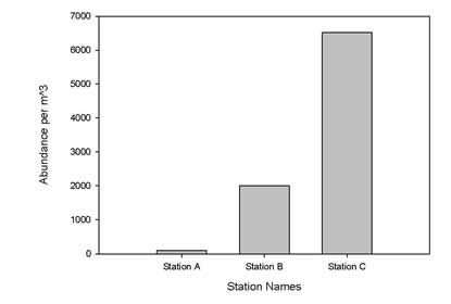
It would appear that the spring phytoplankton bloom had occurred prior to the offshore survey, as there was a significantly lower phytoplankton abundance compared to zooplankton abundance. This suggests that much of the phytoplankton had already been consumed by the large numbers of zooplankton that were discovered in the plankton trawls. Nutrient data from the shoreward side confirmed the homogeneous nature of the water column compared to the data from the stratified side. In addition, the distinction between the two sides of the front was confirmed by calculating Richardson numbers, with the mixed side having an Ri of 0.09 and the stratified side having an Ri of 1.43.
In summary, the waters offshore of Falmouth exhibit the physical, chemical and biological characteristics to be able to determine the boundaries of the tidal frontal system.
Introduction to Geophysics Practical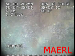 Mawes Harbour, as part of the Fal
Estuary, is a designated Special Area of
Conservation (SAC), due to the presence of
ecologically important biotopes including maerl
and seagrass beds. Both habitats encourage
increased biodiversity, and provide nurseries
for juvenile species, hence maintaining
recruitment rates to adult populations. Mapping
such habitats is an essential step towards
conservation and estuary management. Mawes Harbour, as part of the Fal
Estuary, is a designated Special Area of
Conservation (SAC), due to the presence of
ecologically important biotopes including maerl
and seagrass beds. Both habitats encourage
increased biodiversity, and provide nurseries
for juvenile species, hence maintaining
recruitment rates to adult populations. Mapping
such habitats is an essential step towards
conservation and estuary management.Maerl is a calcareous algae and coloured red by phycoerithrin photosynthetic pigment. It exists as loose beds of branched colonies that interlock, and it is this complicated structure that provides diverse niches for other algae and invertebrates (Foster, 2001). Dead maerl keeps its skeleton, and also provides a similar habitat. Maerl is used as a soil conditioner on acidic soils. Dredging for maerl for this industry has affected stocks in the Fal Estuary (Grall and Hall-Spencer, 2003), so mapping beds is necessary to create legislation that balances economic need with habitat vulnerability. Seagrass is a marine flowering plant that forms ecologically important meadows. As well as providing food for herbivores (Heck and Valentine, 2006), seagrass provides shelter for juveniles and adults (Connolly, 1994; Horinouchi, 2007), and stabilizes sediment in the coastal zone through root systems. It is widely recognised mapping and protecting seagrass is important to promote sustainability of coastal ecosystems (Yap, 2000). Previous studies have successfully used side scan sonar and video analysis to sense seagrass (Norris et al. 1997). The last habitat sampled in the survey was kelp forest, another highly biodiverse habitat (Christie et al. 2003). The fronds provide shelter for nurseries, and a substrate for edible, epiphytic algae; destruction of the algae reduces fish stocks, and impacts top consumers (Lorensten et al, 2010). |

|
|
|
Side Scan Sonar
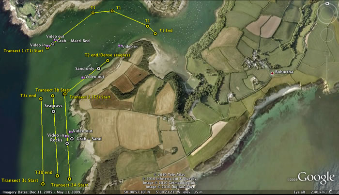
Results Patterns in the side scan output, coupled with ground truthing (grabs and video), were used to identify bottom habitats (see figure 19) The towfish used on Xplorer used two sound signal frequencies. The 100kHz signal had a longer range whereas the 415kHz signal gave a higher resolution image i.e. the 415 kHz signal was able to identify two small objects together on the seabed better than the 100 kHz signal. In order to interpret sidescan images it is necessary to calculate the wavelength of the transmitted sound pulse. This determines the resolution that can be detected from the backscattered sound. The wavelength is determined from: v=fl where: v = velocity of sound in water (1500 m/s) f = frequency of soundwave pulse (Hz) and l = wavelength (m). Layback was calculated by Pythagoras's Theorem. Information from the side scan was plotted in Surfer contour software and used to generate sea floor habitat maps (see figure). As expected, maerl was confirmed in transect one, seagrass and small patches of kelp in transect two, and kelp and seagrass was found in transect three. In more detail, the maerl bed in transect one extended from 184650m East, 32750m North, to past the western limit of the transect. In transect two, the sidescan revealed rocks nearest the shore, giving way to sand, and then seagrass from 18500m East, 32250m North, extending to the eastern edge of the transect. A thin band of kelp was located on the southern border of the seagrass. Finally, in transect three, the seabed was found to be mainly bare sand. Kelp fringed the rocks at 184450m East, 31500m North, 184470m East, 31600m North, and 184450m East, 31850m North. Transect three also revealed a seagrass bed with dimensions 60m by 120m, centred around 184430m East, 31800m North. Transitions in seabed habitat appeared as clear changes of pattern on the side scan output, and so definite boundaries could be plotted on the charts. Due to blurring of the side scan readout along transect one, areas of transect one remained unknown. The video camera was useful in that it provided continuous ground truthing when deployed. It was evident that changes in habitat occured as sharp boundaries occurred rather than a gradient of change (see figure). Video footage of different habitats consistently matched with changes on the sector scan output. |

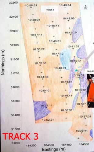
Fig. 19 Habitat map of Transect 3. 
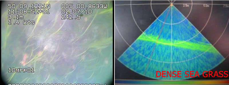
Fig. 20 Dense seagrass shown on sector scan and video. 
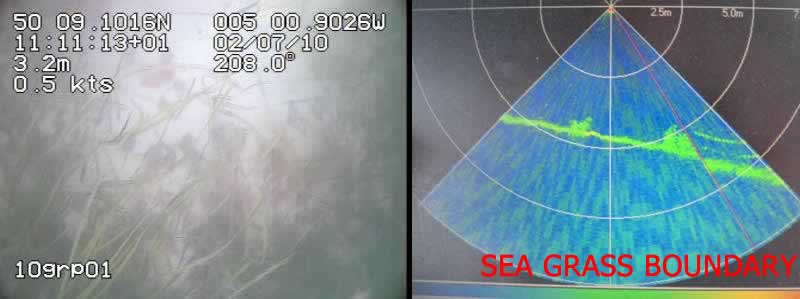
Fig. 21 Seagrass boundary shown on sector scan and video. 
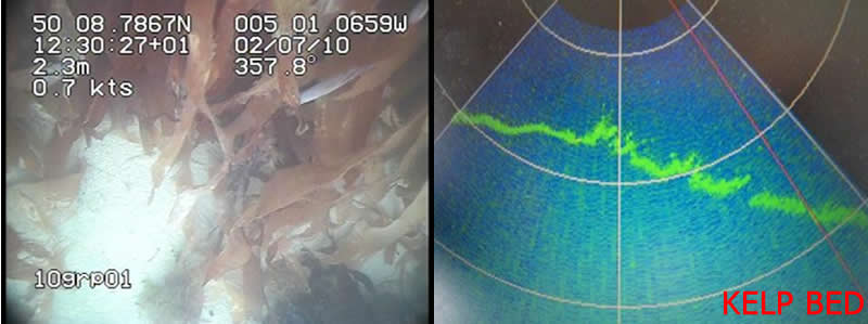
Fig. 22 Kelp bed shown on sector scan and video. |
Sector Scan Sonar
Results The reason for deployment of sector scan sonar was to assess its practicality as a tool for benthic habitat mapping. Whilst side scan sonar can produce wide area sea bed images, interpretation in isolation can sometimes prove problematic. Sector scan sonar can be used to provide a finer analysis of a much narrower swath (Bozzano and Siccardi, 1997). When used in conjunction with other remote sensing techniques, it may be possible to use sector scan images to determine transitions in underwater habitat boundaries that can then be used to calibrate a corresponding feature on a side scan plot. In addition the compact nature and its fixed location on the vessel means that the sector scan sonar can be used in more confined area to target regions of interest for further investigation (unlike a deployed towfish). In transect 2, at 184760m East, 32349m North, dense sea grass was found with the use of a video camera. This corresponded to a thick band of backscatter on the sector sonar data (see figure 20). At 184709E, 032309W, the seagrass bed boundary was identified using the video camera, as seagrass gave way to sand. This corresponded to a sudden change in the sector scan sonar data; a thick band of backscatter was recorded in the area of dense sea grass, and a thinner band was recorded over sand (see figure 21). As small patches of seagrass emerged on the video output, there was small occasional thickening of backscatter data. The sector scan was also able to detect kelp. At 184995m East, 31736m North, sector sonar backscatter became thicker and less uniform; video footage confirmed the transition from bare sand to kelp (see figure 22). The kelp backscatter signature was unique compared to the seagrass backscatter signature, highlighting the potential for sector scan to identify precise benthic habitat. Whilst seagrass was displayed as a thick, uniform band, backscatter off kelp appeared as a rougher band of backscatter seperate from the backscatter received off the bottom. This banding may be due to the relatively dense canopy of kelp fronds overlying a less dense substorey of stalks. On the other hand, there is no canopy in seagrass; seagrass blades are uniformly thick along their length. |
||||||
|
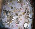
A mechanically operated Van Veen grab provided ground truthing. Samples were washed through a sieve stack for ease of analysis. At grab site 1 (32559E, 184296N), the grab picked up a layer of live maerl on top of fine mud. This information was used to analyse the side scan pattern, and map the extent of maerl. Also present in the grab were hermit crabs, gastropods, ophiuroids, errant polychaetes and green seaweed (Ulva spp.). (Figure 24) Grabs two and three (located at coordinates 31671E, 184503N and 31708E, 184504N respectively) sampled transect three (figures 25 and 26), typified by bare sand and rocks fringed by kelp. The grabs brought up medium coarse sand with shell fragments, bivalves and loose kelp fronds. As discussed in the limitations section, grabbing a kelp bed is difficult due to its patchy nature, and the rock substrate. The spatial difference between sector scan position and grab meant grabs and backscatter did not correlate exactly.
|
Hover over photos to enlarge
|
|||||||
|
Summary of Geophysical
Practical Apart from transect one (due to blurring of side scan image), seabed biota was successfully surveyed, and accurate maps created. Habitats were found where expected; maerl was confirmed at transect one, seagrass and kelp at transect two, and seagrass and kelp were found at transect three. Definite boundaries of habitat were drawn up on charts. Sector sonar data corresponded with video footage and side scan (limitations in comparing video and sector scan are discussed under materials and methods). There is therefore potential to use sector sonar as a habitat mapping tool, although further work would be required to differentiate between a wider range of habitat signatures.
|
||||||||
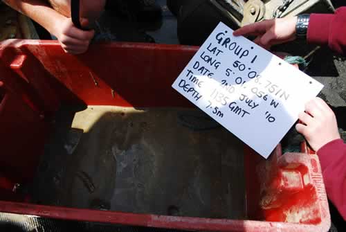
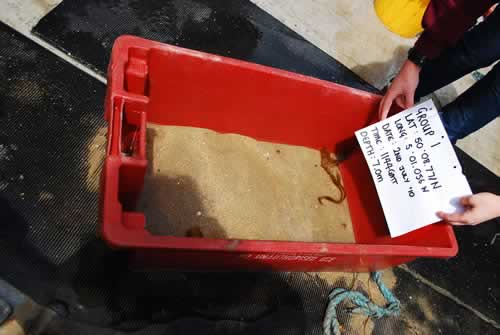
| Station | Latitude | Longitude | Weather | Time (GMT) |
| 1 | 050’08.621 N | 005’01.436 W | Cumulus Cloud 3/8 | 08:41 |
| 2 | 050’10.108N | 005’02.263W | Cumulus Cloud 4/8 | 09:55 |
| 3 | 050’10.979N | 005’01.614W | Cumulus Cloud 6/8 | 10:49 |
| 4 | 050’11.867N | 005’01.939W | Cumulus Cloud 3/8 | 11:40 |
| 5 | 050’12.209N | 005’02.178W | Cumulus Cloud 4/8 | 12:08 |
| 6 | 050'14.451N | 005'00.806W | Alto status 7/8 | 13:12 |
| 7 | 050'13.383N | 005'01.396W | Cumulus and Cirrus Cloud 6/8 | 13:50 |
The Fal estuary is a drowned river valley, or
ria, which formed at the end of the last glacial
maximum (LGM)
approximately 18000 years ago. During
deglaciation, large volumes of glacial meltwater
eroded a deep river valley,
which has since been filled by high present-day
sea-levels. As the glacial freshwater source is
now depleted, the
fresh riverine input into the Fal estuary is
very small, so we expect the estuary to be
tidally dominated with
relatively small horizontal variations in
salinity.
The overall aim of the
survey was to gain an overview of the
physical properties of the Fal
estuary, and to see how these characteristics
affect the chemical and biological properties of
the estuary.
A secondary aim was to classify the estuary in
terms of its physical, chemical and biological
properties. This would be
achieved by producing an estuarine mixing
diagram once all data and water samples were
collected, processed and
analysed. This diagram would enable us to
understand the mixing characteristics of the Fal
estuary in relation to
horizontal changes in salinity.
The survey was to begin at Black Rock and
progress towards the head of the estuary with
the flood tide.
ADCP transects, CTD profiles, and water samples
were to be taken at key points along the main
channel, specifically
at every 0.5 PSU change in salinity. Plankton
trawls were also to be completed at the extremes
in salinity, i.e. at
Black rock, Turnaware point and close to the
riverine end member near Woodbury Point. From
the water samples various
nutrients would be obtained, including nitrate,
phosphate, silicon and dissolved oxygen. The
concentrations of these
nutrients would be determined during lab
analysis of the water samples.


| Salinity Plot from Estuary Practical | ||
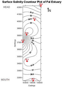
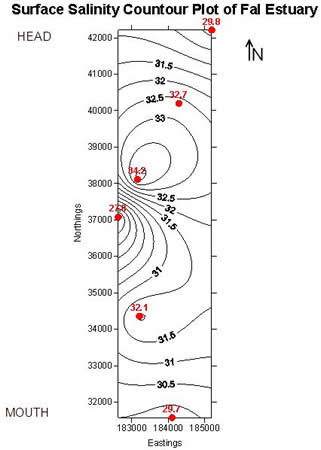
Fig 30. Salinity plot of Fal estuary.
Plan view of the Fal Estuary showing variation in horizontal surface salinity. Values of salinity averaged from surface 1m of CTD profiles. NB - red dots indicate positions of CTD profiles. |
To produce a surface salinity contour plot of the Fal estuary, the average salinity values of the surface 1m of the water column was taken from each CTD profile. This was then related to the position of each CTD drop taken during the survey. The position was then converted from latitude-longitude format to eastings-northings format. Looking at the surface salinity contour plot of the Fal estuary, it is clear that there is very little variation in horizontal surface salinity between the mouth and head of the estuary. The surface salinity varies between 27.8 and 34.2 throughout the entire length of the estuary, indicating that the estuary is relatively well mixed. It is interesting to note, however, that there is a very low value of salinity near the mouth of the estuary (29.7) at CTD drop 1. This region would be expected to have the highest salinity due to its proximity to full-salinity seawater, which was being drawn into the estuary by the flood tide at the time of the survey. The lower salinity could be due to an input of fresh riverine water from St Mawes Harbour on the eastern edge of the estuary. There is also a region of fresher water of salinity 27.8 at CTD drop 3, near Restronguet Point. This is a significant region of freshwater input, like St Mawes Harbour, which could account for this lower salinity. Restronguet Point is also the site of past mining accidents where large quantities of toxic metals were introduced into the estuarine system. As expected, a low surface salinity value is shown at the head of the estuary (29.8) at CTD drop 5. This station was within the main freshwater tributary to the estuary, contributing to a low salinity value in this region. |
|
| ADCP Data from Estuary Practical | ||

 |
 |

 |
|
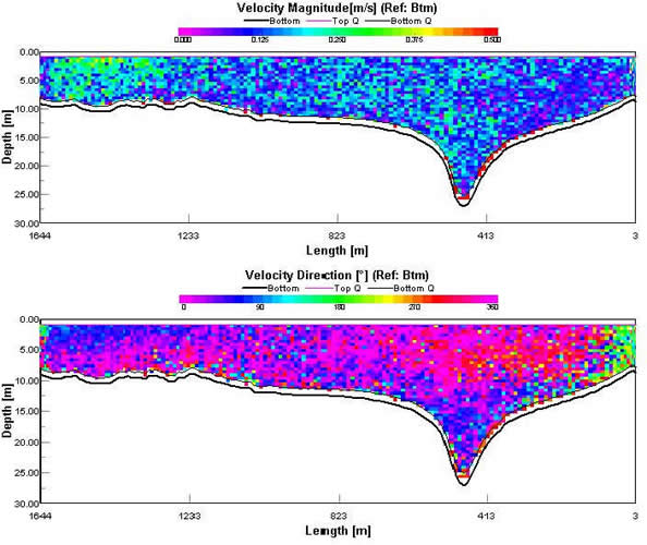
Fig 31. ADCP profile for
transect 1. The ADCP profile of transect 1 was taken across the mouth of the estuary near Black Rock. The average flow rate is around 0.125ms-1, with the lowest flow rates on the eastern side and the highest on the western side. The majority of the flow is in a northerly direction, with a 90o flow in the western side and a flow direction of 180o in the eastern side. |
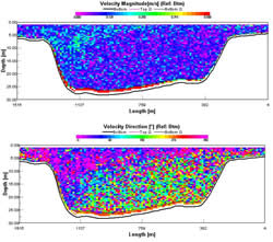
Fig 32. ADCP profile for
transect 2. The ADCP profile of transect 2 shows that there is not a uniform flow throughout the water column but there is a high contra-flow, which is strongest on the eastern side of the channel. The flow rates are generally low, with an average of 0.125ms-1, but the northerly surface flow demonstrates an average higher flow rate of 0.25ms-1, particularly on the western side of the channel. These effects may be due to the effects of the tide turning to a flood tide. |
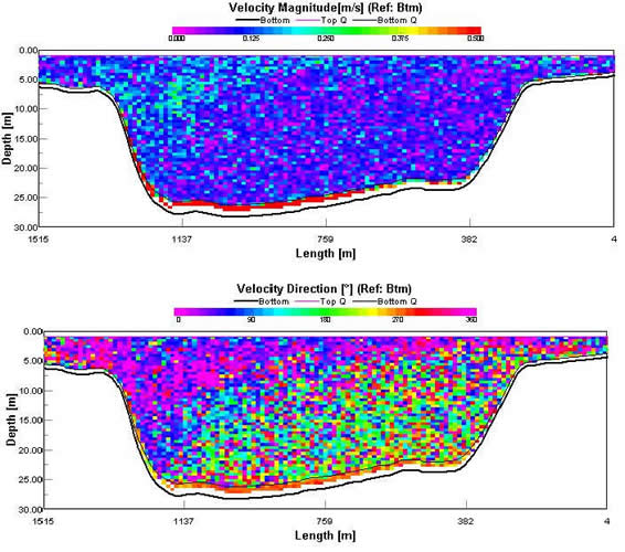
Fig 33. ADCP profile for
transect 3. The ADCP profile of transect 6 was taken at the head of the estuary near Turn Wave Point. The currents here had an average velocity of 0.125ms-1 and demonstrated a very mixed directional pattern. This may be down to the turning of the tide from flood tide to ebb tide, or a greater influence from riverine inputs, or a combination of both. |
| CTD Results from Estuary Practical | ||
|
The CTD data revealed the Fal estuary could be classified as a partially mixed estuary. The estuary was stratified at the head, but well mixed within Carrick Roads. At the top of the estuary, weak tidal action allowed a thermocline and halocline to form; riverine input dominated over weak tidal forces. By the mouth of the estuary, tidal forces dominated the relatively small river input, and the system became mixed.
The CTD profile at station 1 (see figure 35) showed mixed water; temperature and salinity were homogeneous with depth, with salinity at seawater level (34.5). Along the transect, successive stations showed the strengthening of the thermocline and the halocline upstream, until station 6. Station 6 illustrated a stratified system (see figure 34). A permanent and diurnal thermocline combined at station 6 to generate a temperature difference of 3.2 degrees Celsius between the surface and 3.5m. Riverine inputs dominated the weak tidal forces at station 6, which resulted in a halocline from the surface to 2m depth. Surface salinity was recorded at 29, increasing to 32 deeper than 2m. |
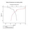
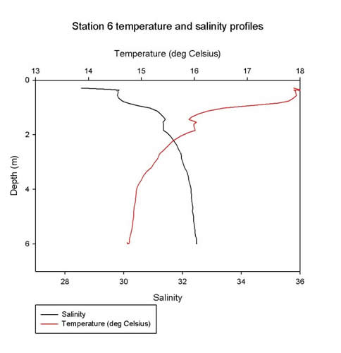
Fig 34. Station 6 temperature and salinity.
|
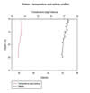
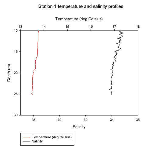
Fig 35. Station 1 temperature and salinity.
|
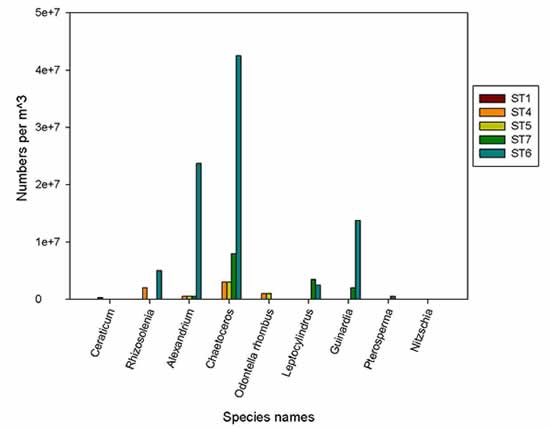
Preliminary analysis of vertical nutrient profiles indicates that nutrient concentration in the water column appears to generally increase towards the head of the estuary.
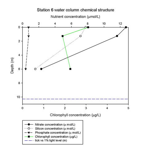
Station 6 (see google earth image, figure 29) represents the furthest upstream sampling point and as expected this had the highest relative levels of nitrate, phosphate and silicon (see figure 37)
.
Vertical nutrient profiles remain
fairly constant through the water column at the mouth of the estuary
reflecting the amount of tidal mixing at these points (see figure 36). As the topography changes at the head of the
estuary to narrower river channels, the effect of tidal mixing
appears to be reduced as the vertical nutrient profiles indicate
some variation, albeit on a small scale.
Chlorophyll concentration in the
estuary follows the low concentrations discovered in offshore
samples indicating that the phytoplankton bloom has occurred
sometime in the past. Again, the highest relative chlorophyll
concentration were identified at the most upstream sampling station.
This is probably the result of the higher nutrient concentrations
there (St6_nut plot]).
The 1% light level depth appears to
increase towards the mouth of the estuary suggesting turbidity
increases in the estuary although this would need to be confirmed
from the turbidity data from the CTD samples.
In summary, the vertical nutrient profiles appear to indicate that the effect of mixing in the estuary decreases with distance from the mouth. Whilst there appears to be some vertical variation in nutrient concentration towards the head of the estuary, the limited number of sampling points and low nutrient concentration values make it difficult to conclude whether this effect has a biological cause or whether it represents some natural variation in sampling or analysis techniques. The vertical profiles would seem to agree with the horizontal profiles that nutrients are being diluted down the estuary by seawater.


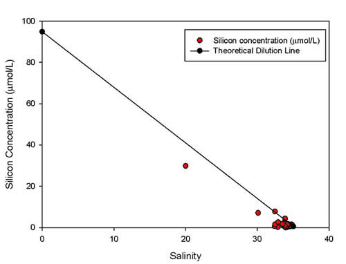
For the silicon mixing diagram, see Fig. 38 the marine end member has a salinity of 34.75 and 0.07 µmol/L of silicon, whereas the riverine end member has a salinity of 0.00 and 94.89µmol/L of silicon. From the location of the sample points with regards to the TDL, it is evident that the silicon displays non-conservative behaviour. The removal of silicon from the surrounding water may be due to biological processes; such as utilisation by diatoms for their frustules, however to confirm this further investigation would be required.

Preliminary analysis of the mixing diagram constructed from the samples taken estuarine practical on 06/07/10 indicates that whilst salinity varies very little along the estuary there would appear that nitrate displays non conservative behavior (see Fig 39). Plotting of the sample points on the mixing diagram indicate a removal of nitrate from solution (fig 39), possible reasons for this may be due to the recent phytoplankton bloom utilizing the nitrate for metabolic processes.
Nitrate enters the marine environment via runoff from the land, and is then diluted as it is mixed. The highest nitrate values were found at station 6 (Max value 12.86 µmol/L), which corresponds to the furthest upstream location where samples were taken. This is what was expected.

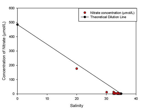
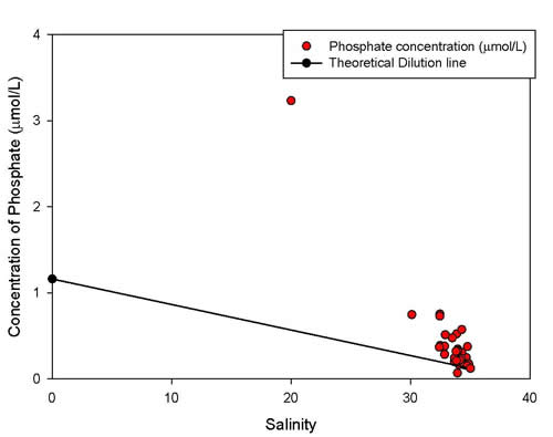
Fig. 40 is an estuarine mixing diagram for phosphate concentration (µM) with riverine and marine end members connected by a theoretical dilution line.
Values for the riverine end member were salinity 0.00 and phosphate 1.16 µmol/L, at the marine end member values of salinity 35.02 and 0.12 µmol/L of phosphate were recorded. The majority of samples collected on RV Conway on the 06/07/10 were in the salinity range of 30.11 and 35.02
Water column depth restricted the range of RV Conway thus the samples at the top of the estuary were collected by ribs. Plotting the data on the mixing diagram revealed an input of phosphate (recorded value 3.23 µmol/L) at a salinity of 20.00, which was a sample given to us in the lab previously collected by the technicians. Phosphate is showing non-conservative behaviour as the points reside above the theoretical dilution line, so addition of phosphate is occurring. At salinity 20.00 there appears to be an outlier, which will need further investigation to determine the input source of phosphate at this point.

|
Phytoplankton
Zooplankton
|
The Falmouth field course provides an opportunity to explore the physical, chemical and biological characteristics of the Fal from offshore to estuary head. Although the course week was divided into three distinct data collection voyages, it is possible to draw some overall conclusions of the area.
The Fal estuary appears to be a partially mixed estuary that flows out into the Western approaches. It was characterised by a thermocline and halocline evident at the head of the estuary that diminishes towards the mouth. This suggests that the mixing influence of the tides decreases up the estuary.
As the estuary transitioned into open ocean, the homogeneous water column structure evolved into a distinctly stratified structure. This is indicative of a tidal mixing front located offshore. The characteristics of the mixed and stratified sides of the front allowed its extent to be mapped to some degree.
As was expected, the source of nutrients would appear to be from the river inputs along the Fal where concentrations were highest. Nutrient concentration decreased down the estuary and offshore suggesting dilution by mixing seawater away from the source.
The low chlorophyll concentrations and low numbers of phytoplankton recorded in the estuary and offshore suggest that the expected temperate spring/summer phytoplankton bloom had occurred at some point prior to the course. This supposition was supported by the relatively high numbers of zooplankton present in the estuary and offshore that would have fed on the bloom.
In 2003 the Fal was a candidate Special Area of Conservation as a result of features such as the maerl beds and seagrass meadows found in St. Mawes bay. Given the vulnerability of these features, accurate mapping of their extent is of vital importance. By referencing side scan sonar output and video, it would appear feasible to be able to use sector scaning sonar as an aid to identifying changed in benthic habitat.
The Fal and its surrounding area offers distinct oceanographic and biological features for marine scientists to study. In time, it may be possible to use the datasets collected to provide an in depth analysis of the physics, chemistry and biology of this unique area.
Potential further work
To extend this investigation other facets of the fal estuarine system and related offshore regions could be analysed in greater detail.
In the offshore regions more detailed mapping could be undertaken to get a more accurate positioning of features such as the frontal system, as well as taking a longer term time series of the front to see how it changes over time and the effects this has. Utilisation of satellite data can augment the data collected in the field to gain a better understanding of the features in this area. Another index number which could be used is the Simpson-Hunter index to aid in determining the front. A look into the turbidity of the water column and how it changes over time could also be considered. On the biological side a more detailed look at the standing stock of plankton could be embarked on, in particular a study into the change in biomass over time and the relationship with nutrient distribution. An examination of the controls and limits on primary productivity could also be considered. A useful aid for this would be the L4 and E1 buoys offshore from Plymouth from the western channel observatory, which provides data on nutrient fluxes and chlorophyll concentrations.
In the fal estuary further study could be undertaken to understand the effects of the different river systems on the estuary. The flushing times and its effects on nutrients, contaminants and pollutants could be examined, as well as the residence times. A longer term time series could be initiated to investigate the changes in the estuary, including the effects of the tide. Further investigation into the physical processes could be undertaken and the Richardson Number could be calculated at various points along the estuary to indicate whether the estuary is well mixed, partially mixed or stratified. Similarly to the offshore work, turbidity could be studied to try to understand the effects this could have on the estuarine system, with particular regard to the biology. An examination of the controls and limits on primary productivity could also be considered as well as a study into the change in biomass over time and the relationship with nutrient distribution. A further investigation could combine the data from both within the estuary and offshore to look at gradients from the top of the estuary to the related offshore regions.
On the geophysical side, a more detailed mapping project could be undertaken to gain a greater understanding of the extent of the various habitats in the region. A long term time series could be used to investigate how the extent of habitats, such as seagrass, changes over time and a look into the possible reasons for this. The sector scanner could be utilised on more habitat types to see if there is a significant change on the read out, which could be useful to find out if it could be used as a more prominent instrument for mapping various different types of habitat.
Click to download any of the following files
to save and open on your own computer.
| Processed data files | Raw data files | |||
| File name | Description | File name | Description | |
| LB_FINAL.docx | LOG BOOK (typed up) | |||
| Boat_work2.kmz | Google Earth file of all boat work | |||
| OFFSHORE FILES | chlorP.xlsx | Processed chemical Lab work | Plk_ trl.xlsx | Plankton data from stations. |
| N2P2.xlsx | St1&9.xlsx | |||
| phosP.xlsx | St4.xlsx | |||
| Proc_O2.xls | St1_sum.xlsx | Raw data organised by station # | ||
| Proc_Si.xlsx | St4_sum.xlsx | |||
| St1_cal.xlsx | CTD data imported into Microsoft Excel with calibrations | St9_sum.xlsx | ||
| St2_cal.xlsx | ||||
| St3_cal.xlsx | ||||
| St4_cal.xlsx | ||||
| St5_cal.xlsx | ||||
| St6_cal.xlsx | ||||
| St7_cal.xlsx | ||||
| St8_cal.xlsx | ||||
| St9_cal.xlsx | ||||
| GEOPHYSICS FILES | Relf_all.srf |
Surfer documents Contour plots of transects |
||
| Sds_all.srf | ||||
| ESTUARIES FILES | estchemP.xlsx | All stations processed nutrient data | PhytoR.xlsx | Plankton raw excel files |
| O2P.xlsx | ZooR.xlsx | |||
| T1ADCPP.JPG | ADCP Plots | ADCPdirR.txt | ADCP Directory | |
| T2ADCPP.JPG | CTD_DIRR.txt | CTD Directory and raw CTD Files | ||
| T3ADCPP.JPG | CON0945R.txt | |||
| T4ADCPP.JPG | CON0956R.txt | |||
| T5ADCPP.JPG | CON1140R.txt | |||
| T6ADCPP.JPG | CON1223R.txt | |||
| T7ADCPP.JPG | CON1320R.txt | |||
| CTD1_CP.xlsx | CTD Data imported into Microsoft Excel spreadhseets | CON1418R.txt | ||
| CTD2_CP.xlsx | CON1510R.txt | |||
| CTD3_CP.xlsx | ||||
| CTD4_CP.xlsx | ||||
| CTD5_CP.xlsx | ||||
| CTD6_CP.xlsx | ||||
| LIGHTP.xls | Processed light data for estuary | |||
Bozzano R. and Siccardi A., (1997). Underwater vegetation detection in high frequency sonar images: A preliminary approach. Lecture notes in computer science, Vol 1311/1997, pp 576-583.
Christie, H., Jorgensen ,N.N., Norderhaug, K.M., Waage-Nielsen, E., 2003. Species distribution and habitat exploitation of fauna associated with kelp (Laminaria hyperborean) along the Norwegian coast. Journal of the Marine Biological Association of the United Kingdom 83, 687-699.
Connolly, R.M., 1994. A comparison of fish assemblages from seagrass and unvegetated areas of a southern Australian estuary. Marine and Freshwater Research 45, 1033-1044.
Dyer,K.R. (1973) Estuaries: A Physical Introduction 2nd Edition.John Wiley & Sons Ltd, England.
Foster, M.S., 2001. Rhodoliths: Between rocks and soft places – Minireview. Journal of Phycology 37, 659-667.
Grall, J., Hall-Spencer, J.M., 2003. Problems facing maerl conservation in Brittany. Aquatic Conservation: Marine and Freshwater Ecosystems 13, S55-S64.
Head, P.C., 1985, Practical estuarine chemistry, Cambridge University Press, Cambridge.
Heck, J.K.L., Valentine, J.F., 2006. Plant-herbivore interactions in seagrass meadows. Journal of Experimental Marine Biology and Ecology 330, 420-436.
Hodgkiss,I.J, Lu SH (2004) The effects of nutrients and their ratios on phytoplankton abundance in Junk Bay, Hong Kong. Hydrobiologia 512: 215-229.
Heiskary,S., Markus,S. (2001) Establishing, Relationships Among Nutrient Concentrations, Phytoplankton Abundance, and Biochemical Oxegen Demand in Minnesota, USA, Rivers. Journal of Lake and Reservoir Management, 17(4), 251-262.
Horinouchi, M., 2007. Distribution patterns of benthic juvenile gobies in and around seagrass habitats: effectiveness of seagrass shelter against predators. Estuarine, Coastal and Shelf Science 72, 657-664.
James, R. and Wright, J. 2005, Marine biogeochemical cycles, 2nd Ed, Elsevier Butterworth-Heinemann, Oxford.
Lorentsen, S., Sjotun ,K., Gremillet, D., 2010. Multi-trophic consequences of kelp harvest. Biological Conservation doi: 10.1016/j.biocon.2010.05.013.
Martin-Jézéquel, V., Mark Hildebrand, M., and Brzezinski, M.A.(2003) SILICON METABOLISM IN DIATOMS: IMPLICATIONS FOR GROWTH . Journal of phycology . Vol 36 I(ss 5) Pgs 821-840.
No Author. (2006) ‘Nutrients -- Nitrogen and Phosphorus’:From Voluntary Estuary Monitoring Manual Chp 10: Available http://www.epa.gov/owow/estuaries/monitor/pdf/chap10.pdf. Accessed 06/07/10.
Norris, J.G. Wyllie-Echeverria, S. Mumford, T. 1997. Estimating basal area coverage of subtidal seagrass beds using underwater videography. Aquatic Botany 58, 269-287.
Roubeix, V., Rousseau, V. and Lancelot, C. 2008, Diatom succession and silicon removal from freshwater in estuarine mixing zones: From experiment to modelling, Estuarine, Coastal and Shelf Science. Vol 78, Iss 1:14-26.
Sharples, J., & Simpson, J. (2009). Shelf Sea and Shelf Slope Fronts. Encyclopaedia of Ocean Sciences , 391-400.
Yap, H.T., 2000. The case for restoration of tropical coastal ecosystems. Ocean and Coastal Management 43, 841-851.


