
Joanna 'semi-colon' Kerr Matthew 'take the piss out of jo' Young Felix 'Carl Zeiss' Smith Joseph 'bandana man' Onoufriou Francis Samuel 'fun time' Faldo-Hassard III
Simon 'i bugger off to weddings' Taylor Simon 'the baguette' Laugier Emma 'chill your beans' Cross
The effects of physical and chemical processes on the biota of the Fal Estuary and surrounding waters
![]()
![]()
![]()
![]()
![]()
![]()
![]()
|
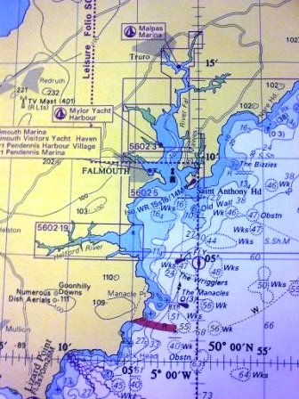
Figure 1.1: Map of Falmouth and surrounding area. [click image for chart]
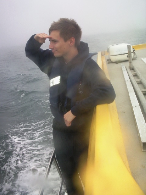
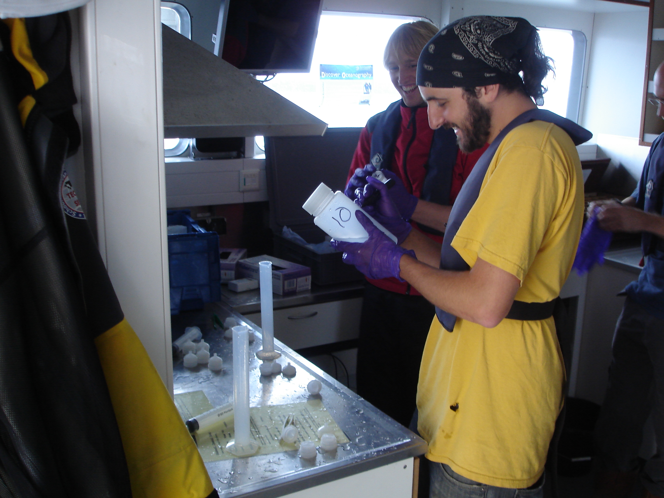
Figure 1.3: Scientist hard at work |
The Fal Estuary (Figure 1) was formed 18,000 years ago at the end of the last glacial maximum. Rising sea levels, coupled with low sedimentation rates caused the river valley to flood. This lead to formation of a drowned river valley or Ria, common to the South-West of England. Typical features of a Ria include a long narrow estuary with branching small rivers; the Fal is supplied by 6 main tributaries and 28 smaller creeks. The Fal is the third largest natural harbour in the world by volume, with the deepest section, Carrick Roads, reaching 34m at chart datum. The estuary displays many characteristics associated with well mixed regions including: - Low fluvial inputs leading to tidal domination - A V-shaped basin - Extensive sand and mud flats in the inter-tidal zone Due to the estuaries' diverse structure, it has been designated a Special Area of Conservation (SAC) and Site of Special Scientific Interest (SSSI). Extensive maerl beds, containing the species Phymatolithon calcareum and Lithothamnion corallioides, can be seen in the lower Fal and represent the largest beds in South-West Britain. These create an environment that is essential for the survival of some rare epifaunal and infaunal species such as the Couch's goby (Gobius couchi). Estuarine sediments can form major sinks for contaminants released during industrial activity. Increased concentrations of arsenic, copper, tin and zinc can be seen within the Fal estuary, with the highest concentrations at Restronguet creek on the Western side of the Estuary. The long term increase in metal concentration has resulted in certain benthic invertebrates becoming resistant, explaining their relative dominance over susceptible species. The aim of the research is to sample and analyse the coastal and estuarine waters, in and around the Fal, in order to further understand the complex processes that are involved in the functioning of this diverse region. This was achieved by analysing CTD and ADCP data inline with samples taken at various stations offshore and within the estuary for biological and chemical properties. The aim of the geophysical survey was to determine the benthic habitats of the Fal Estuary by use of a Geo Acoustics 415kHz side scan sonar, Van Veen grab and underwater camera. The data were interpreted with respect to biological and physical properties.All times are given in GMT, all latitude and longitude values are given in WGS84. |
![]()
|
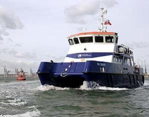
RV CALLISTA
Figure 2.1: RV Callista RV Callista is a catamaran style vessel. With 3 deployment points, including a large ‘A’ frame, it is well equipped for offshore research. The vessel also houses dry and wet labs, allowing a range of sample collection and analysis methods to be performed on location. |
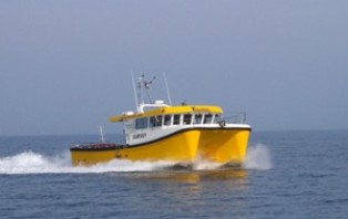
XPLORER
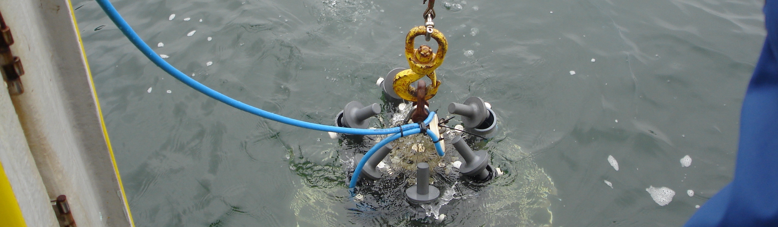
Figure 2.2: Xplorer The Xplorer is a fast, stable, highly manoeuvrable vessel making it ideal for estuarine and offshore work. It contains a full complement of oceanographic equipment including a rosette with CTD and Niskin bottles, the deployment of which is aided by a crane on the rear deck. A Van Veen Grab and plankton net are also available. |
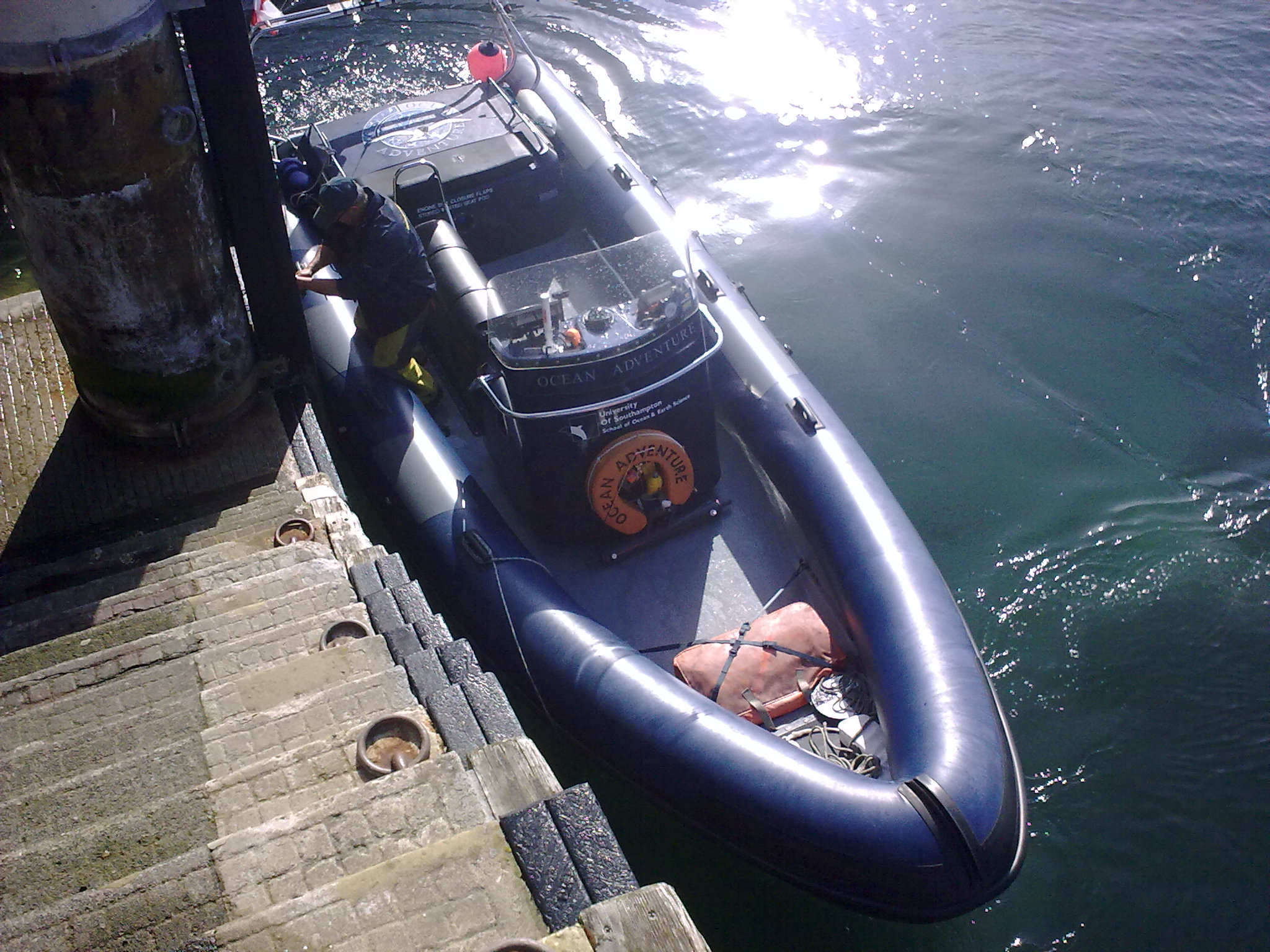
OCEAN ADVENTURE
Figure 2.3: Ocean Adventure RIB Ocean Adventure is a Rigid Inflatable Boat (RIB). RIBs are fast and maneuverable vessels with a small passenger capacity. They are very useful for travelling up estuaries to shallower regions which are inaccessible to larger boats due to their larger drafts. |
|
Length: 19.75m Breadth: 7.40m Draft: 1.80m Depth Midship: 2.85m ‘A’ Frame: 4 tonne Capacity Capstan: 1.5 tonne pull 2x Side Davits: 100kg each |
Length: 12.00m Beam: 5.20m Draft: 1.20m Heila deck crane with winch Hydraulic capstan: 1 tonne Survey Equipment mounting brackets Max Speed: 25 knots Cruising Speed: 18 knots |
Length: 7.00m Beam: 2.55m Draft: 0.5m Max Speed: 35 knots Cruising Speed: 25 knots Max Endurance: 1 day at sea Range: 100nm |
![]()
|
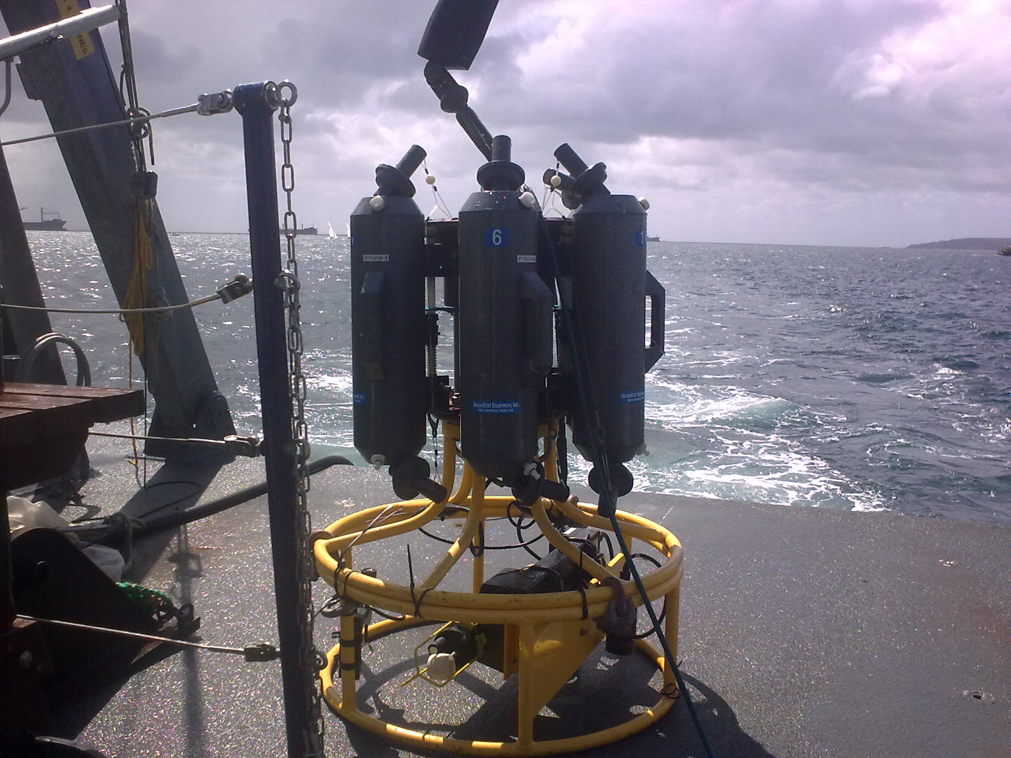
CTD AND ROSETTE
Figure 3.1: CTD and Rosette |
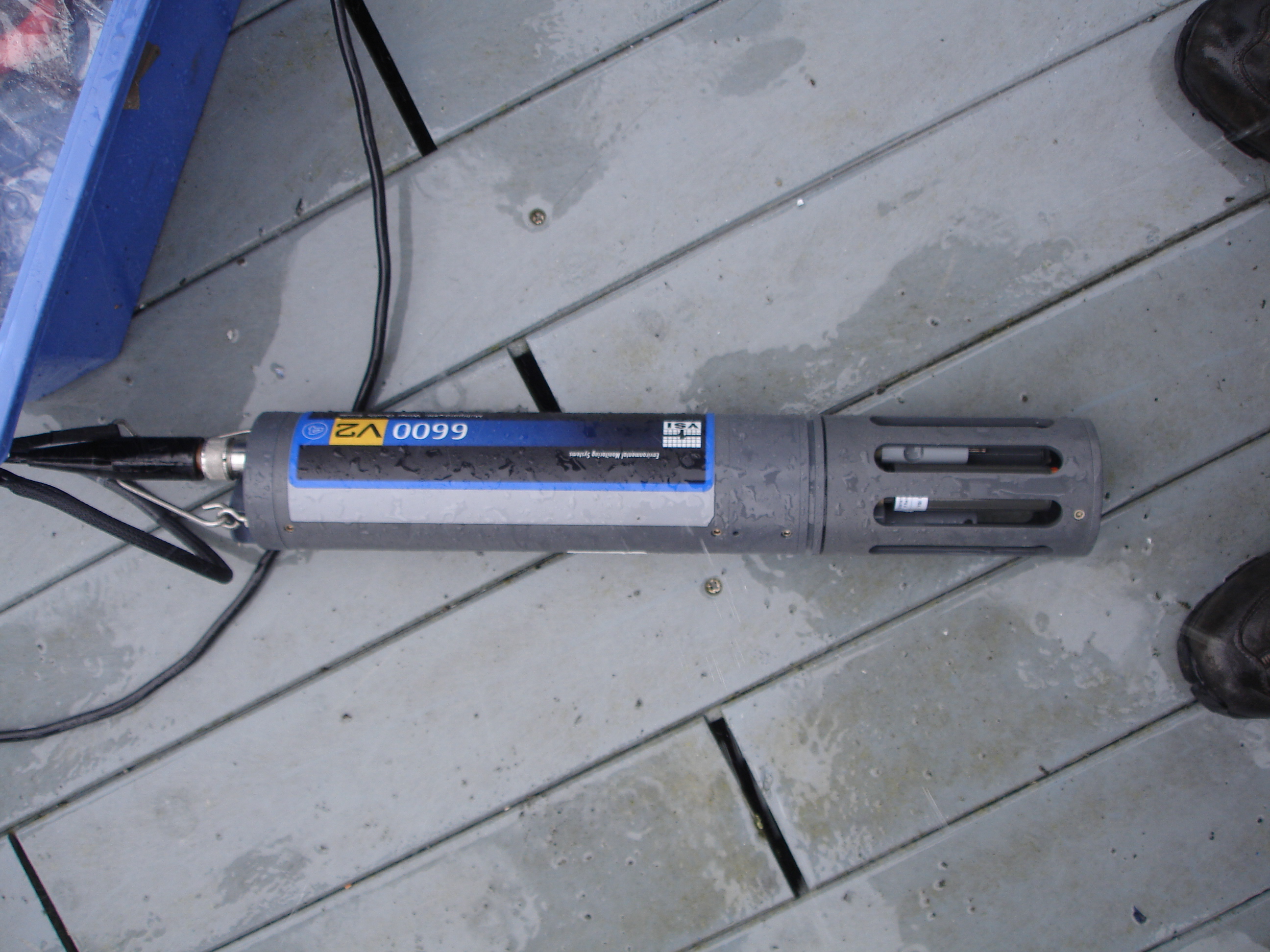
YSI PROBE
Figure 3.2: YSI Probe |
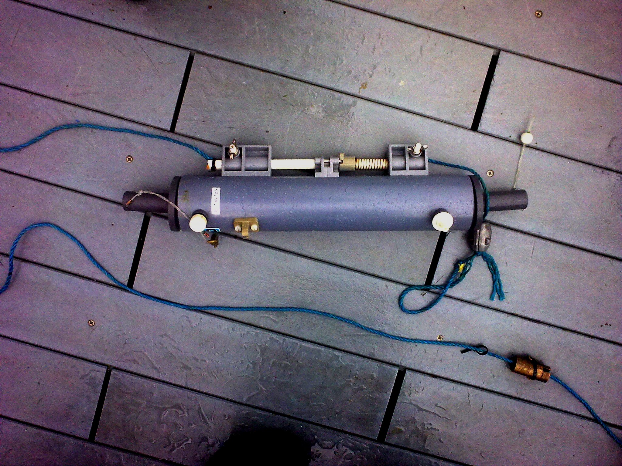
NISKIN WATER BOTTLE
Figure 3.3: Niskin Water Bottle |
|
A CTD is used to take vertical profiles of the water column by continuously measuring conductivity (as a proxy for salinity), temperature and depth. It is usually mounted onto a rosette where equipment such as Niskin sampling bottles, fluorometers and transmissometers can be mounted to measure various oceanographic parameters. |
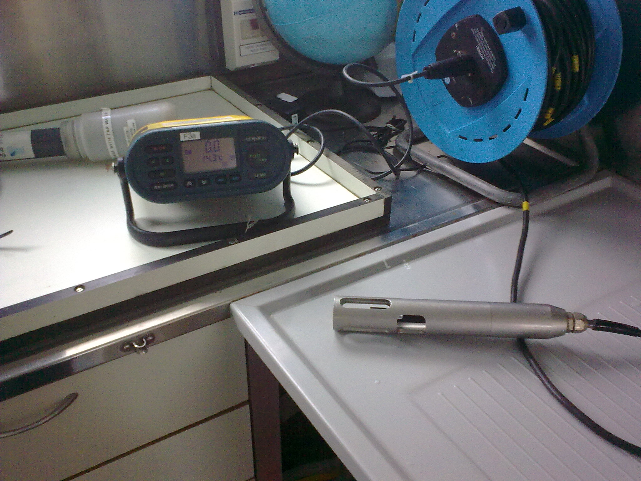
The Yellow Springs Instruments (YSI) Probe is a multi-sensor probe which can continuously measure vertical changes in depth, temperature, salinity, dissolved oxygen and pH. Deployable from most sampling stations including vessels and pontoons, all parameters can be read from a hand-held digital display. |
Niskin bottles can be used to collect water samples at a range of depths. Samples collected are useful for analysis of nutrient, dissolved oxygen and chlorophyll concentrations. Whilst open at both ends and attached to a hydroline it can be lowered through the water column to the desired sampling depth. Once the depth is reached the bottle can be closed with the aid of either a messenger sent down the hydroline or electronic messengers located onboard the vessel. |
|
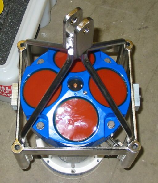
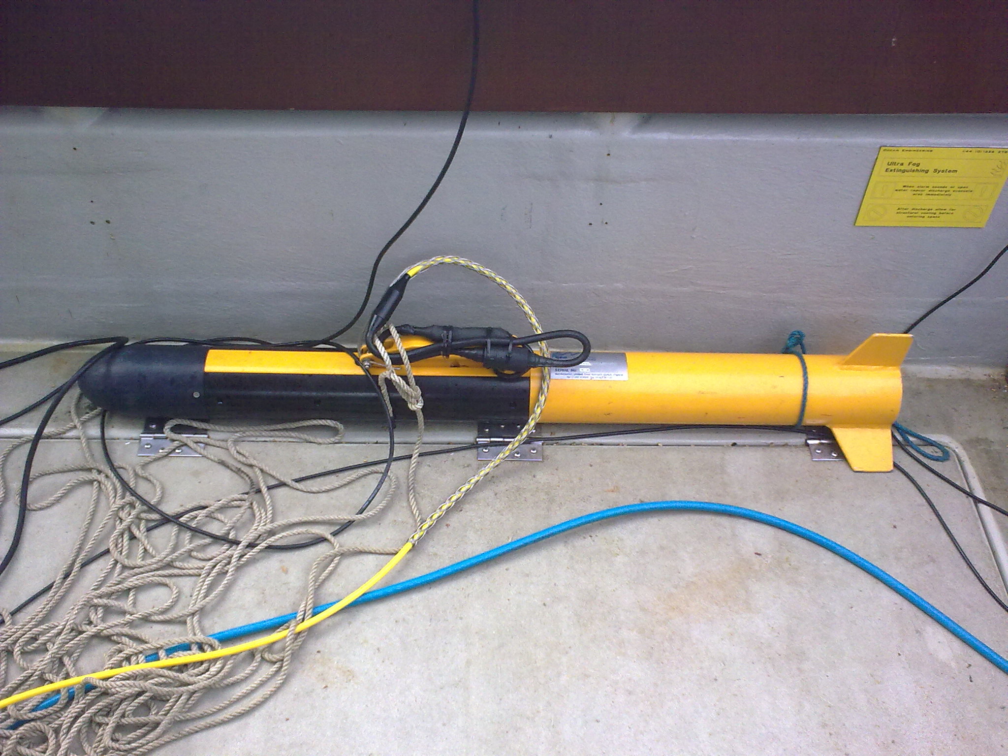
ADCP
Figure 3.4: ADCP |
TEMPERATURE/SALINITY PROBE
Figure 3.5: Temperature/Salinity Probe |
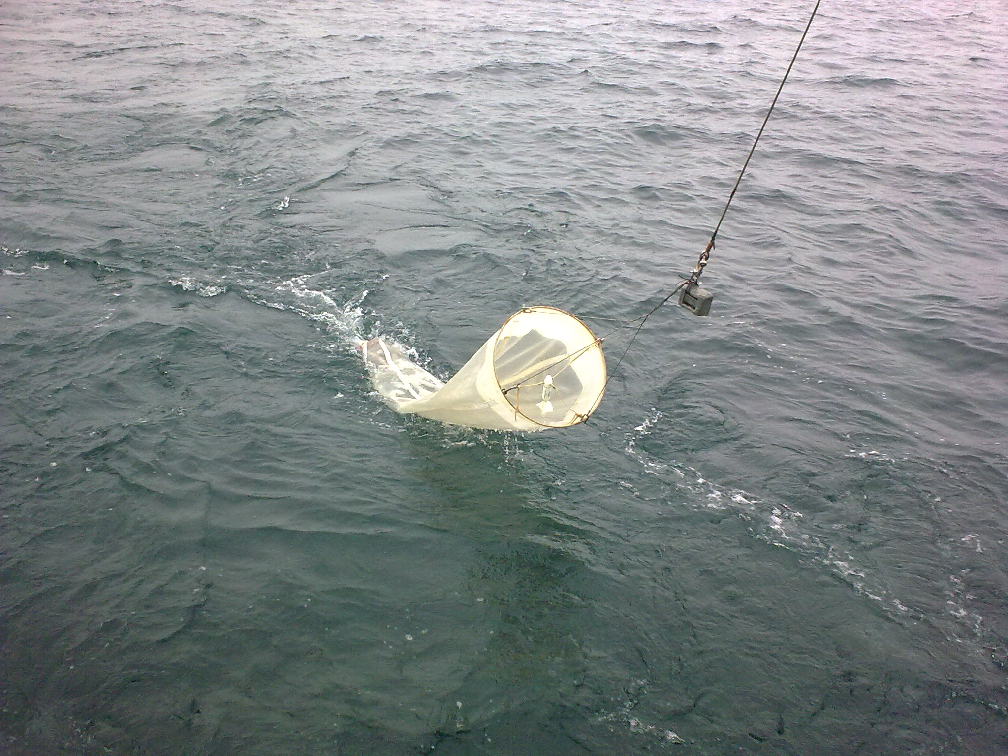
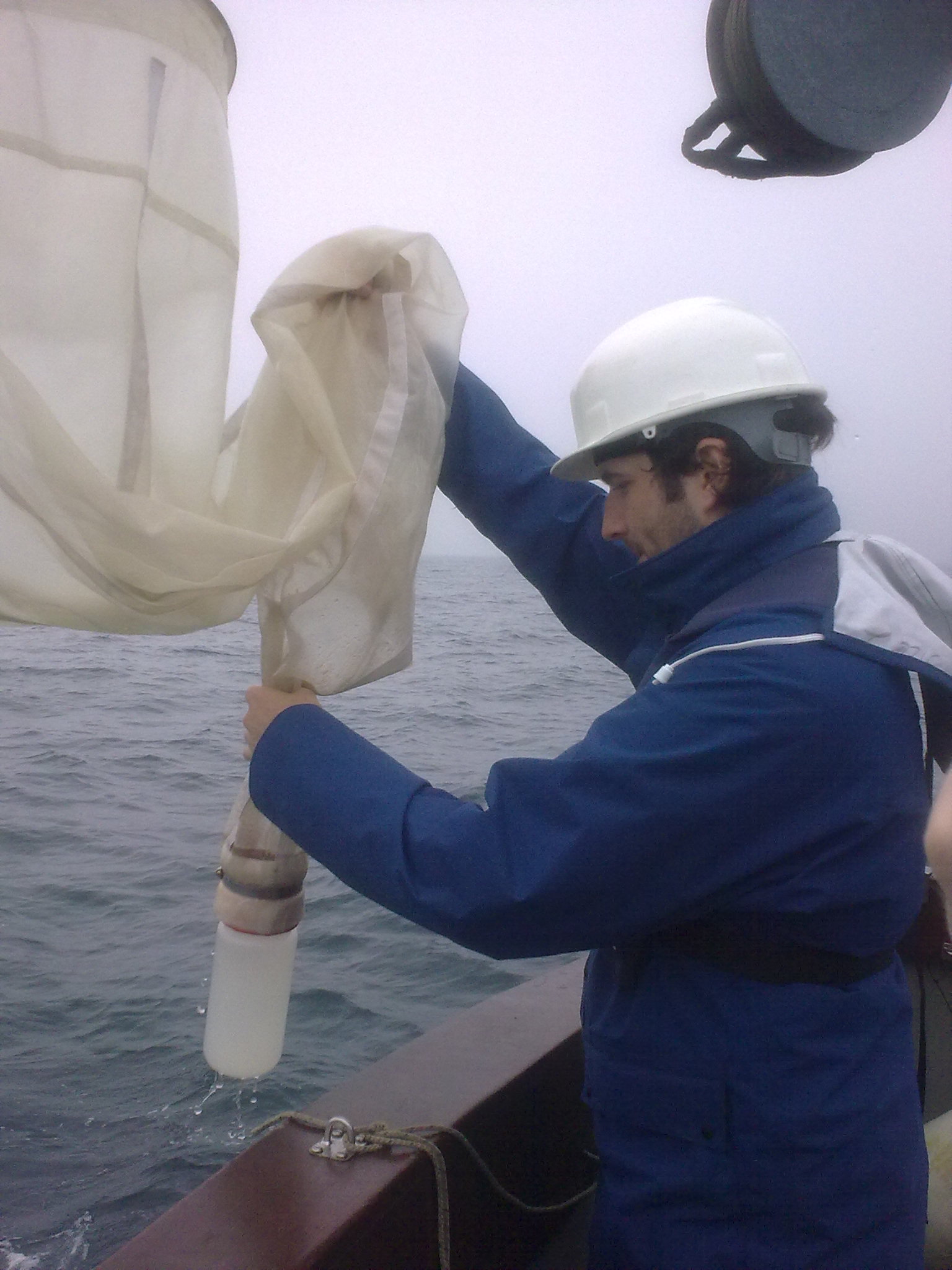
PLANKTON NET
Figure 3.6: Plankton Net |
|
Acoustic Doppler Current Profilers (ADCP), use sound waves in the form of sonar to detect current velocities. They utilize transducers which emit pulses of mono-frequencies in known directions and measures Doppler shift. This ultimately produces a graphical output which must then be interpreted. |
The T/S probe is an instrument that is used to measure temperature and salinity within a body of water. They contain built in thermisters which measure temperature via resistance. As the temperature increases the resistance is reduced producing a measure of temperature in °C. Salinity is measured through automatic analysis of the current strength passed between two electronic diodes. It is a conductive system. |
Plankton nets can vary in mesh size (200um in the instance of this report). They are used to collect zooplankton during a trawl and are equipped with an impellor with a five digit counter to record the volume of water filtered. Contents are pushed towards the distal end, where a collection vessel is located. |
|
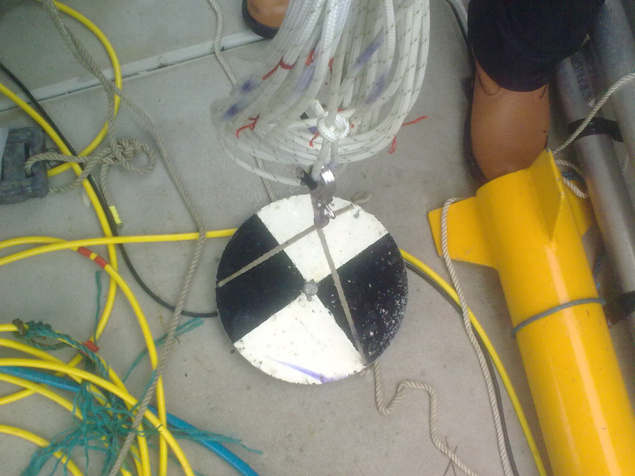
SECCHI DISK
Figure 3.7: Secchi Disk |
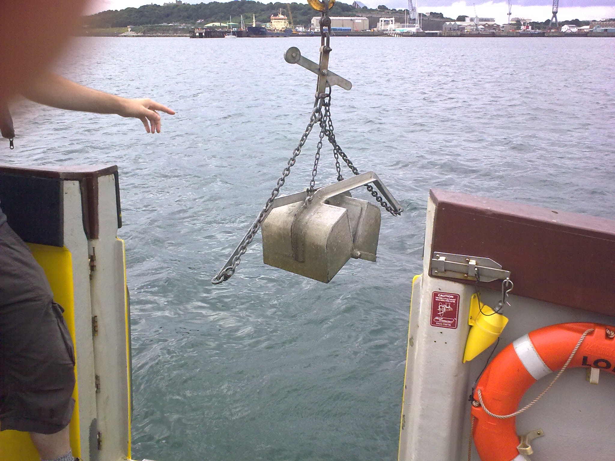
VAN VEEN GRAB
Figure 3.8: Van Veen Grab |
SIDESCAN SONAR
Figure 3.9: Sidescan Sonar |
|
Used to measure the surface light penetration, Secchi disks can be lowered from most vessels and sampling stations. The euphotic zone can be calculated as three times the depth at which the Secchi disk can no longer be seen with naked eye. This is used only as a rough guide as to the depth of the euphotic zone as the method is highly susceptible to human error. |
Van Veen Grabs are mechanical grabs which can be used to analyse the biology of the benthic environment. Subsequent sieving of grab samples can aid the identification of sediment composition and benthic fauna. |
Sidescan Sonars are usually mounted on a fish which is towed behind a vessel. The 415 kHz device has a 150m swath width and produces a graphical interpretation of the topography of the seafloor. A pulse is emitted and the return signal is interpreted by the time difference between emission and recieval. Areas of strong return correspond to steeper slopes facing the side scan sonar. Areas of weak return correspond to flatter areas. Where there is no return, slopes which are steeper than the angle of the incident beam are present. |
|
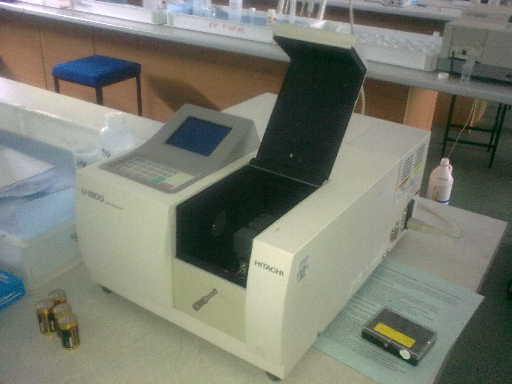
Hitachi U-1800 SPECTROPHOTOMETER
Figure 3.10: U-1800 Spectrophotometer |
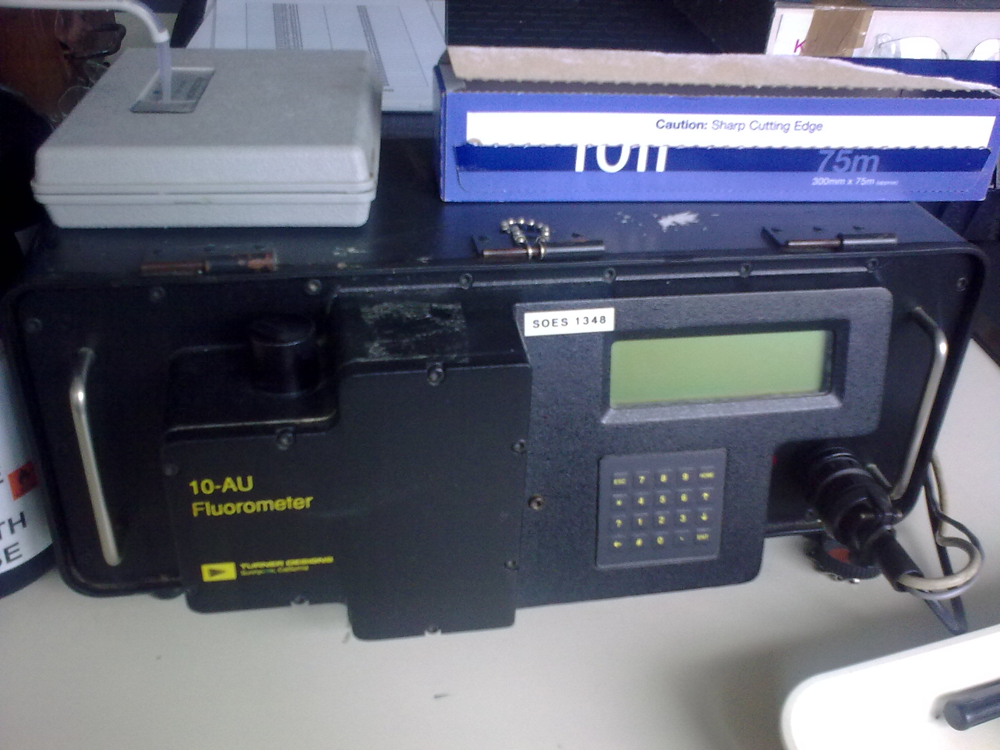
10 AU FLUOROMETER
Figure 3.11: 10 AU Fluorometer |
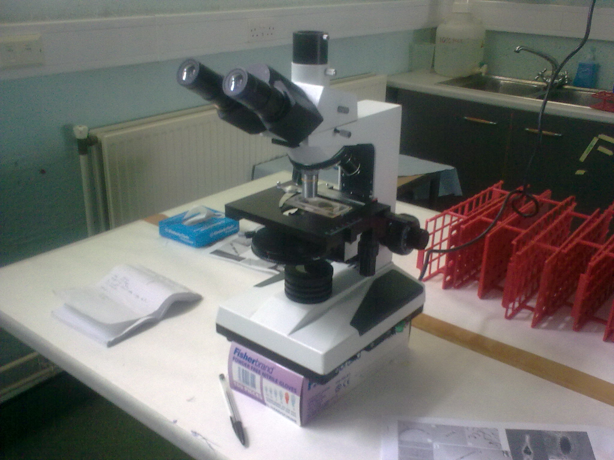
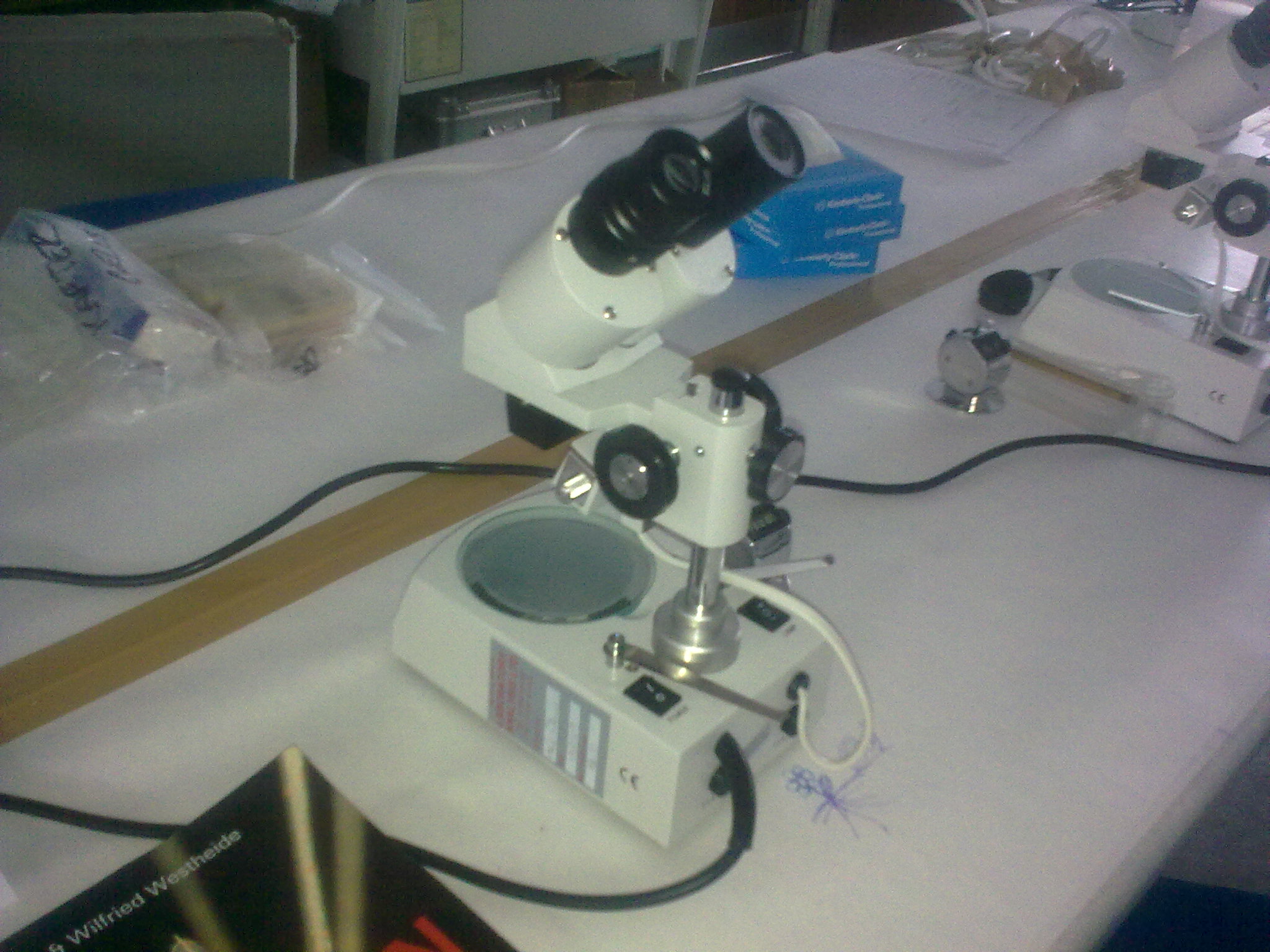
MICROSCOPES
Figure 3.12: |
|
A spectrophotometer is a device that measures light intensity by measuring the wavelength of light passing through a given medium. Spectrophotometers have a range of spectral bandwidths however the specific bandwidth used for any given analysis is dependent on the substrates or medium being investigated. |
A Fluorometer is used to measure fluorescence intensity as well as wavelength distribution after excitation by a certain spectrum of light. Specific molecules within a medium can be identified using these parameters. Some fluorometers can detect fluorescent molecule concentrations down to 1 part per trillion. |
Microscopes were used to identify phytoplankton and zooplankton species and measure abundance. Dissection microscopes (left, figure 3.12) can be used to count and identify zooplankton, while light microscopes (right, figure 3.12) can be used to count and identify phytoplankton. |
![]()
![]()
![]()
![]()
![]()
![]()
![]()
|
||
|
This report aims to investigate the interactions of physical, chemical and biological processes in the Fal estuary. Samples were taken using a CTD deployed from the vessel Xplorer at four stations from the mouth of the estuary (Black Rock) to Smuggler's Cottage in the River Fal. Further samples were taken from the pontoon at King Harry Ferry. |
||
|
Figure 4.2: Plankton net in action
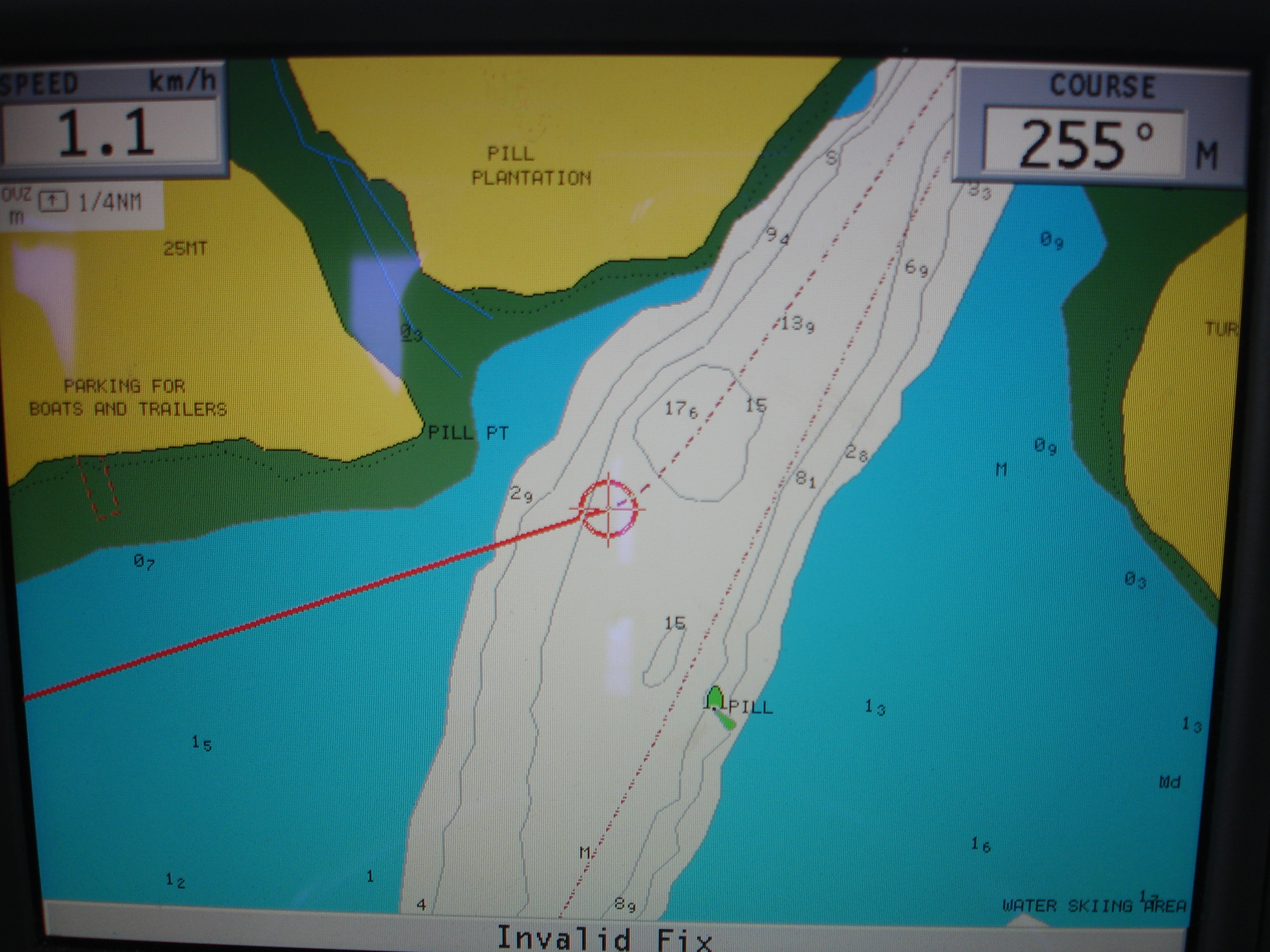
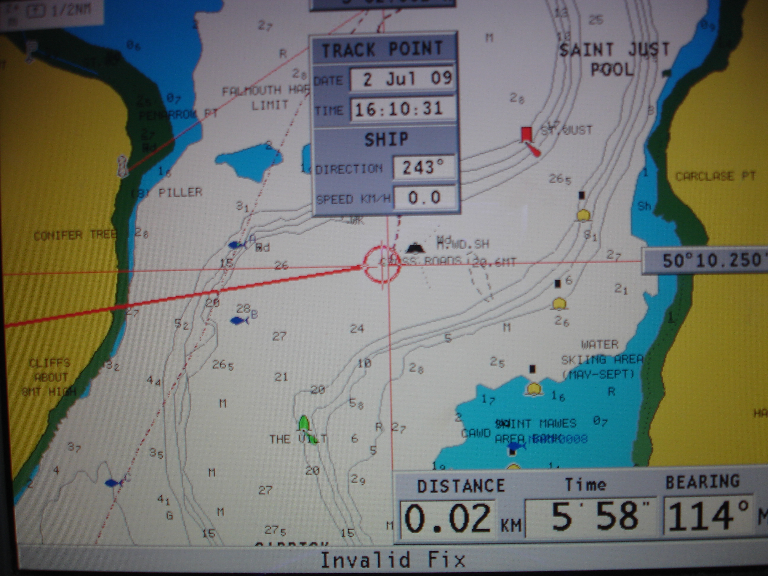
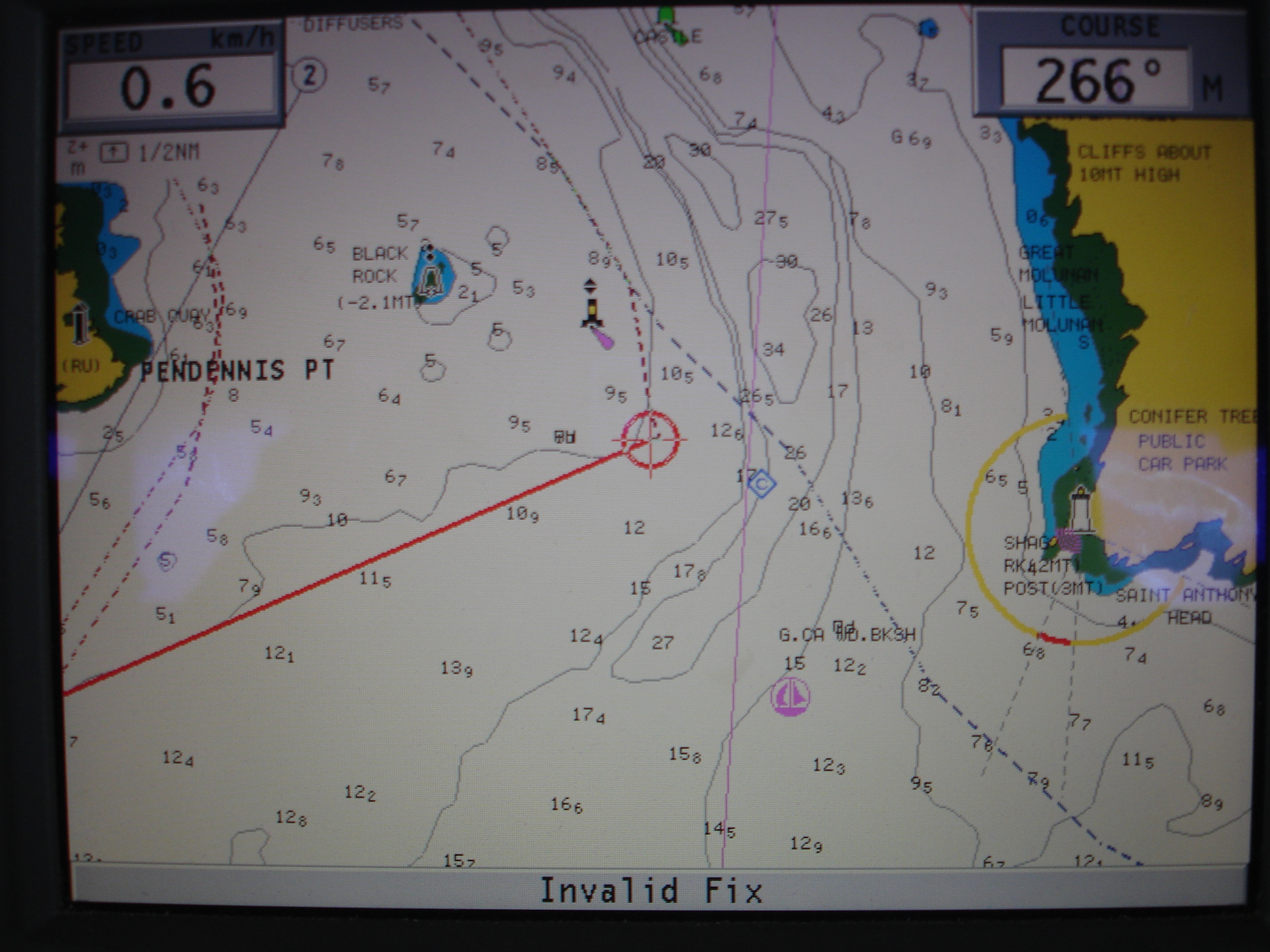
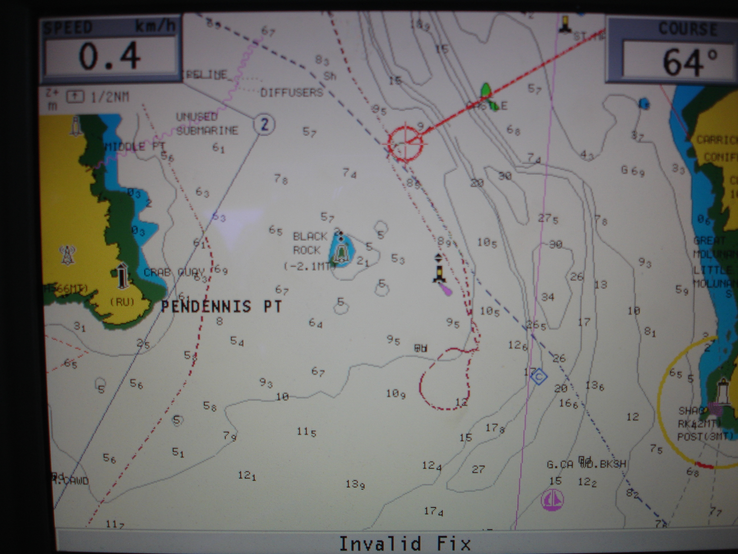
Figure 4.3: Xplorer chart position for Station 1
Figure 4.3: Xplorer chart position for Station 1
Figure 4.3: Xplorer chart position for Station 1
Figure 4.3: Xplorer chart position for Station 1 |
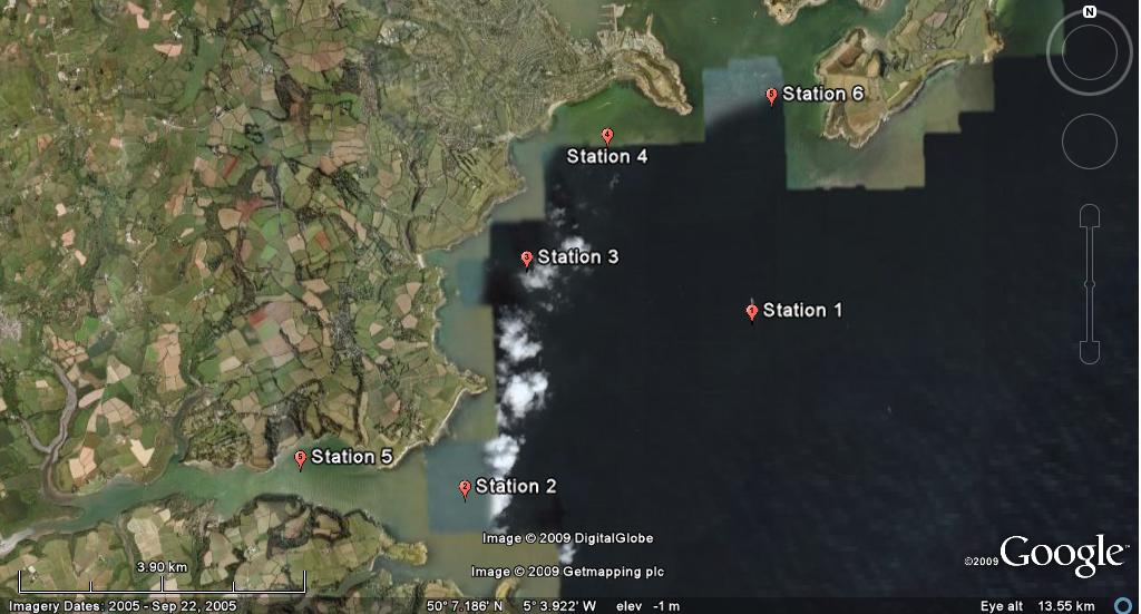
FIELD METHODS:
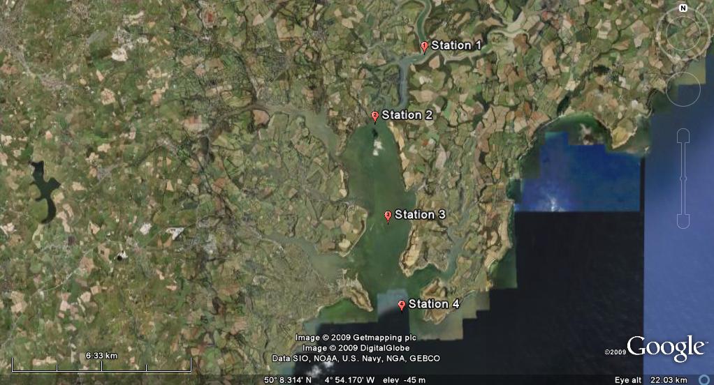
[Figure 4.1: Google Earth Map showing Station Positions for Xplorer Survey] PONTOON Data were collected between 09:38 and 11:40 from the Pontoon at the King Harry Ferry (050°13.000 N; 005°01.550 W). Temperature, salinity, pH and oxygen saturation measurements were taken every 30 minutes at 0.5m intervals from the surface to approximately 5m. A YSI probe was employed for these measurements. Water samples were taken using a 5 litre Niskin bottle every 60 minutes at the surface and at 4m. The water samples were analysed in the lab for nitrate, phosphate, silicate and oxygen concentrations. Nutrient subsamples were filtered using GFF filters with a pore size of 0.7µm and stored at 4°C. The Filter papers were retained and stored in acetone for the purposes of chlorophyll measurements. Winkler bottles in which the oxygen samples were stored were kept underwater to avoid addition of O2 from the atmosphere. Water samples for nutrient analysis were stored in glass bottles with the exception of samples intended for silica analysis which were stored in LDPE bottles to prevent contamination from the silica in the glass. XPLORER The Xplorer survey commenced at Smuggler's Cottage (050°13.521 N; 005°00.956 W) at 13:53. This was adjusted to 050°13.476 N; 005°01.023 W at 14:11 GMT due to the initial location being too shallow. The final station was at Black Rock (050°08.560 N; 005°01.637 W), where surveying began at 15:38. A further two stations at 050°12.186 N; 005°02.437 W and 005°02.437 N; 005°02.437 W were also sampled. Three sets of water samples were collected using 2.5L Niskin bottles mounted onto a rossette. At each location a bottom, surface and intermediate depth was sampled with three subsamples collected from each Niskin bottle. These were later analysed for nitrate, phosphate, silica and oxygen concentrations in the same way as the samples collected on the pontoon. Two 5 minute plankton trawls were conducted using a 54cm diameter net with a 210 μm mesh size. The sites sampled were at King Harry Ferry, followed by Black Rock. Trawls were conducted at these points in order to compare zooplankton species abundance and diversity at the extreme ends of the estuary. The samples were fixed with 10% formalin solution so that the species could be identified and counted in the lab. Further plankton samples were taken from surface waters, via Niskin bottles. These samples were fixed with Lugol's iodine. A Secchi disk was deployed at the 5th station (050°08.912 N; 005°01.834 W) in order to determine the depth of the euphotic zone. The secchi desk depth was 8.5m which suggests a Euphotic Zone depth of 25.5m. CTD information was taken using a GO Rosette with seabird CTD. Fluorometer and seatech transmissometer readings were taken at the same depths as the water samples
|
|
|
(CLICK IMAGES TO ENLARGE)
Figure 5.1: Estuarine Mixing Diagram of Nitrate/Nitrite concentration with increasing salinity from Smuggler’s Cottage to Black Rock. Data were collected on 02/07/2009. Samples that are below the detection limit of the apparatus (0.1µM) are plotted as 0.0µM.
Figure 5.3: Estuarine mixing diagram for silicon in the Fal Estuary between Truro and Black Rock. Data were collected on the 2/07/2009 on board RV Xplorer.
Figure 5.5: Estuarine Mixing Diagram for Phosphate with increasing salinity from Smuggler’s Cottage to Black Rock. Data was collected on 02/07/2009. Samples that are below detection limit of the apparatus (0.03 µM) are plotted as 0.0µM
Figure 5.7: Dissolved oxygen concentrations across depths of 0-15m between Smuggler's Cottage and Black Rock
Figure 5.9: Chlorophyll Data for 4 stations between Black Rock and Smuggler's Cottage at depths to 16m |
NITRATE Nitrate concentration ranged from a 410.0µM/l riverine end member to a seaward end member of less than 0.1 µM/l. Using an estuarine mixing diagram, a Theoretical Dilution Line (TDL) was plotted between the two end member concentrations (figure 5.1). The TDL shows that nitrate concentration is inversely proportional to salinity; nitrate concentration increases with decreasing salinity up the estuary. Data points in the seawater end, from salinities of 26.66 to 35.19, fall significantly below the TDL, suggesting removal from the system. The apparent removal of nitrates indicates non-conservative behaviour. SILICON Silica concentration values ranged from a 1.67 µM/l seaward end member to a 126.30 µM/l riverine end member. The greatest silicon concentration was recorded at 14m depth at station 1 where levels reached 5.77 µM/l. The smallest value was recorded at station 4 at 5.9m depth where concentration was 0.08µM/l. Stations 1,2 and 4 displayed their lowest silica concentrations at intermediate depths with values of 2.08, 2.41 and 0.08 µM/l, respectively. Conversely, the lowest concentration recorded at station 3 was 1.21 µM/l at 15.2m depth. It can be seen from the TDL that with increasing salinity, silicon concentrations decrease (figure 5.3). Silicon can be assumed to be behaving non-conservatively as data points at the seaward end fall below the TDL, implying silicon removal from the system. PHOSPHATE Phosphate concentrations decrease with increasing salinity down the estuary, from a 0.41 µM/l riverine end member to a 0.00 µM/l seaward end member. Samples collected ranged from 0.263 µM/l at station 1 to 0.002 µM/l at station 4. The data shows addition toward the seaward end of the estuary with most points plotting above the TDL. The estuarine mixing diagram therefore suggests that phosphate is behaving non-conservatively in the estuary. DISSOLVED OXYGEN Dissolved oxygen satuartions vary from 99.4% (station 2) to 113.2% (station 3) across depths of 0 – 15 metres between Smuggler's Cottage and Black Rock (Figure 5.7). Each station showed decreasing saturation levels with increasing depth. This is exemplified by Station 2 which demonstrated the greatest variation between surface and deep samples with a difference of 12.2% across a depth range of 13.2 metres. Station 4 showed little change in saturation level throughout the water column with a negligible increase of 0.6% between 1.2 and 12.2 metres. Anomalies are apparent at station 2. Prior to a large decrease, saturation levels increase between 1.3 and 3.8 metres by 0.5%. Station 2 also shows an anomalously low saturation level of 99.4%. The YSI probe time series data indicates a large increase in oxygen saturation in surface waters up to 1 metre depth (figure 5.8). Between 1 and 3.5 metres depth, levels remain relatively constant at an average saturation of 104.9% before decreasing again to reach an mean saturation of 103% at 5 metres depth. The standard deviation of the Winkler samples to the YSI probe data ranged between 0.71% and 1.77% indicating a high degree of accuracy. CHLOROPHYLL All stations have a chlorophyll maximum just below the surface. At stations 1 and 2 there was a dramatic decrease in chlorophyll at 5 meters (figure 5.9). The CTD data from these stations suggests a thermocline at this depth, caused by the stratified nature of the water column. Chlorophyll at stations 3 & 4 decreased linearly with depth (figure 5.9). These values correspond with fluorometer values (figure 8.3, 8.4) however there are anomalies which have been attributed to faults with the fluorometer rather than acetone values Salinity is a conservative measure of mixing and as such makes a stable proxy for analyzing changes in chlorophyll. The highest recorded chlorophyll of 7.8 µM/l was at a Salinity of 33. The lowest recorded chlorophyll was 2.5 µM/l at a salinity of 34 at 4m depth.
|
(CLICK IMAGES TO ENLARGE)
Figure 5.2: Eulerian time series of changes in Nitrate plus Nitrite concentration with increasing salinity of measurements taken at a Pontoon at King Harry Ferry, Falmouth on 02/07/09 between 0938 to 1138 GMT (flooding tide)
Figure 5.4: Eulerian time series of changes in silicon concentration with salinity. Measurements taken at King Harry Ferry Falmouth on 2/07/2009 between 09:38 and 11:38 GMT (flooding tide)
Figure 5.6: Eulerian time series of changes in Phosphate concentration with increasing salinity of measurements taken at a Pontoon at King Harry Ferry, Falmouth on 02/07/2009 between 0938 and 1138 GMT (flooding tide)
Figure 5.8: Dissolved oxygen concentration at depths at the Pontoon
Figure 5.10: Changes in chlorophyll concentration μM/L with salinity between Black rock and Smuggler's Cottage. |
|
[click images to enlarge]
Figure 6.1: Average abundance of phytoplankton species collected from surface waters between Smugglers Cottage and Black Rock (station 2, (14:38): 050°12.186 N; 005°02.437 W, station 3, (15:09): 050°10.275 N; 005°02.048 W, station 4, (15:38): 050°08.560 N; 005°01.637 W) ; Carrick Roads Falmouth; 02-07-09.
Figure 6.3: Average abundance of zooplankton species (m-3) collected from surface waters near Smugglers Cottage (start, 14:21: 050°13.385 N; 005°01.459 W finish, 14:26: 050°13.139 N; 005°01.559 W) and Black Rock (start, 15:56: 050°08.4499 N; 005°01.662 W finish, 16:03: 050°08.789 N; 005°01.800 W); Carrick Roads, Falmouth; 02-07-09.
Figure 6.5: Relative abundances of Diatoms to Dinoflagellates at station 3 (050°10.275 N; 005°02.048 W). Data collected on 02/07/09. |
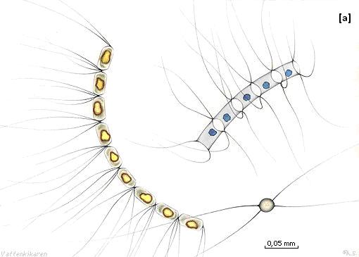
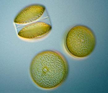
PHYTOPLANKTON Figure 6.1 shows the structure of the phytoplankton community in the Fal Estuary at each of the sampled stations: stations 2, 3 and 4. Figure 6.2 shows the relative abundance of phytoplankton species. The greatest populations were shown at stations 2 and 3 with average counts of 62000 individuals/L and 57000 individuals/l, respectively. Station 4 showed the lowest population with only 11000 individuals/l. Stations 2 and 3 were strongly dominated by Diatom species, in particular Chaetocerus, with low numbers of Dinoflagellates and Flagellates also present (Figures 6.4 and 6.5). Station 4 showed Dinoflagellates to be the most abundant group but did not dominate to the same degree as seen in the other two stations (Figure 6.6).
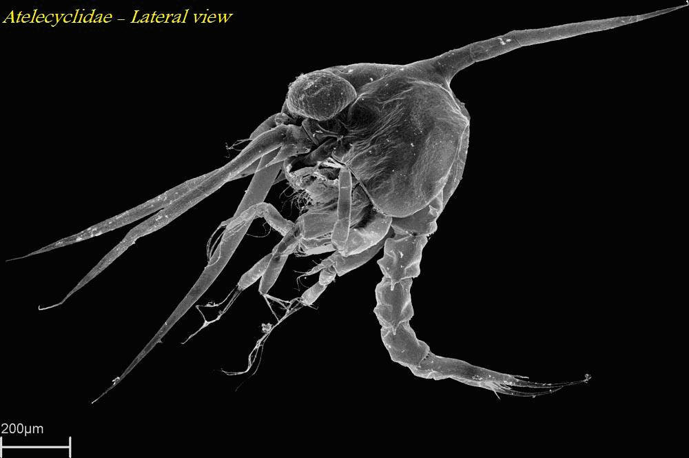
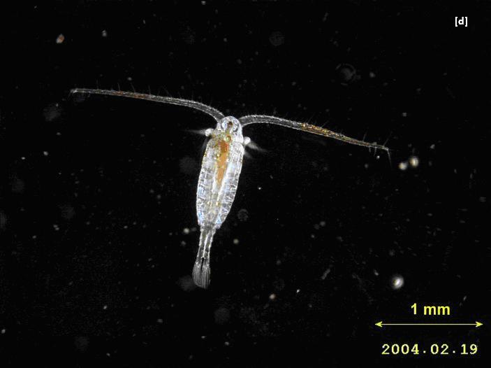
Figure 6.4: Common Phytoplankton and Zooplankton Species. Far left: Chaetocerus; dominant at Stations 2 and 3, Middle Left: Coscinodiscus; dominant at Station 4, Middle right: Decapoda larva, Far right: Copepoda ZOOPLANKTON Figure 6.3 shows the structure of the zooplankton community at stations 1 and 4. Both stations showed a low abundance of zooplankton with only 112.5 numbers/m3 at station 1 and 182.5 numbers/m3 at station 4. These low levels at station 4 coincide with the low phytoplankton levels and therefore suggest the cause of the low zooplankton abundance. Since no phytoplankton data were collected at station 1, no comparison of relative abundance can be drawn.
|
[click images to enlarge]
Figure 6.2: Relative abundance of phytoplankton species collected from surface waters between Smugglers Cottage and Black Rock (station 2, (14:38): 050°12.186 N; 005°02.437 W, station 3, (15:09): 050°10.275 N; 005°02.048 W, station 4, (15:38): 050°08.560 N; 005°01.637 W); Carrick Roads Falmouth; 02-07-09.
Figure 6.4: - Relative abundances of Diatoms to Dinoflagellates at station 2 (050°12.186 N; 005°02.437 W). Data collected on 02/07/09.
Figure 6.5: Relative abundances of Diatoms to Dinoflagellates at station 4 (050°08.560 N; 005°01.637 W). Data collected on 02/07/09. |
|
ADCP Data from the ADCP were aquired on 4/07/2009 by group 5 as it was not operational on 2/07/2009, when the remainder of the data was collected. It must be noted here that, due to heavy rainfall during this period, the flow velocity may have been affected. High tide was at 15:04 GMT therefore data was collected on a flooding tide. All data were collected from the main channel (Carrick Roads) from station 1 at Restronguet Creek to the Inner Harbour area. Station 1 (14:35-14:41, 050°12.157 N, 005°02.804 W to 050°12.147 N, 005°02.123 W) shows an area of higher flow velocity (4-5m/s) at the bed of the estuary. A similar trend can also be observed at station 3, the data being collected from 14:46-14:51 (050°12.267 N, 005°02.370 W to 50°12.185 N, 005°02.115 W). Flow velocities vary over the entire estuary however, as opposed to just by the bed as at station 1. Station 4 was recorded on slack water between 15:56 and 16:13 at the mouth of the estuary (050º08.490, 005º01.096 to 050º08.612, 005º02.456). A marked increased in velocity at the surface can be seen at this site. |
(CLICK IMAGES TO ENLARGE)
Figure 7.1: ADCP Plot for Station 1
Figure 7.2: ADCP Plot for Station 3
Figure 7.3: ADCP Plot for Station 4
Figure 8.2: CTD Data for Station 2, showing Salinity, Temperature, Fluorescence, Phosphorus, Silicon, Nitrate, Transmission and Chlorophyll with depth.
Figure 8.4: CTD Data for Station 4 showing Salinity, Temperature, Fluorescence, Phosphorus, Silicon, Nitrate, Transmission and Chlorophyll with depth
Figure 8.6: Longitudinal temperature profile between Smugglers Cottage and Black Rock (Carrick Roads, Falmouth). Distances along the x-axis are in Km with Smugglers Cottage at x=0. Blanking files have been applied to remove unreliable data. Vertical columns of stars represent data acquisition points on CTD downcast. |
||||||||||||||||||||||||||||||
|
(CLICK IMAGES TO ENLARGE)
Figure 8.1: CTD Data for Station 1, showing Salinity, Temperature, Fluorescence, Phosphorus, Silicon, Nitrate, Transmission and Chlorophyll with depth.
Figure 8.3: CTD Data for Station 3 showing Salinity, Temperature, Fluorescence, Phosphorus, Silicon, Nitrate, Transmission and Chlorophyll with depth.
Figure 8.5: Longitudinal salinity profile between Smugglers Cottage and Black Rock (Carrick Roads, Falmouth). Distances along the x-axis are in Km with Smugglers Cottage at x=0. Blanking files have been applied to remove unreliable data. Vertical columns of stars represent data acquisition points on CTD downcast.
|
CTD
CTD cast 1 (Smugglers Cottage): temperatures recorded ranged from 18.9°C to 17.25°C (0m : 14.2m) whilst salinity ranged from 26 to 35. CTD cast 2 (Carrick Roads): temperatures recorded ranged from 18.5°C to 16.4°C (0m : 14.6m) whilst salinity ranged from 26 to 36. CTD cast 3 (Carrick Roads): temperatures recorded ranged from 18°C to 17°C (0m : 14.6m) whilst salinity ranged from 34.5 to 35. CTD cast 4 (Carrick Roads): temperatures recorded ranged from 17.9°C to 16.9°C (0m : 12.2m) whilst salinity ranged from 26 to 36. CTD casts were made at 13:53, 14:38, 15:09 and 15:38, with a high tide of 4.4m at 14:10. Station 1 displays a sharp decrease in salinity from the surface down to approximately 1m, followed by a sharp increase down to 2m. Past 2m depth a gradual increase ensues up to 14m (figure 8.1). Station 2 also demonstrates a variable salinity in the upper 2m, however the increase in salinity with depth is much more gradual than at station 1 (figure 8.2). This trend changes once again at station 3, with a sharp increase in salinity at approximately 5m depth and once again at 9m (figure 8.3). Station 4 , taken from the mouth of the estuary, displays a very sharp increase in salinity from approximately 1-1.25m with little variation from 1.25-10m (figure 8.4). Temperature profiles demonstrate a similar trend at all four stations, with an overall decrease with depth, however the depth of the thermocline increases from station 1-4. This increase in depth is approximately 2m at each station. Fluorescence shows little change with depth at all stations. This can be attributed to the fact that sampling was not undertaken below the euphotic zone; the euphotic zone was determined by secchi disk depths which did not exceed 6m. Transmission at station 1 shows a steady decrease in turbulence with increasing depth, from 4.258V at the surface to 4.250V at 14m. Station 2 shows a completely different trend to that seen at station 1 with turbulence remaining constant at 4.31V between the surface and 4m before increasing dramatically to 4.45V at 6m. Turbulence then remains constant at 4.45V down to 15m. A small amount of noise is shown at this station. A similar trend is observed at station 3 with turbulence remaining constant at 4.44V between the surface and 4m depth before again, increasing dramatically between 4m and 6m to 4.51V. Turbulence then again remains unvarying at 4.51V to depth (15m). Station 4 shows a very slight linear increase in turbulence with depth from 4.513V at the surface to 4.528V at 12m. A large amount of noise was recorded at station 4 which made interpretation difficult. Figure 8.6 shows that temperature decreases from estuary head to estuary mouth, similarly, figure 8.5 shows that salinity range decreases towards the distal end of the estuary. Minimal thermal stratification is evident at all CTD cast stations, indicating a well mixed water column even at the proximal end of the estuary. Longitudinally, from estuary head to mouth, there is a general trend for isotherms to deepen. This can be observed, for example, with the 17.4°C isotherm which deepens from 4.8 to 10.4 m between Smugglers Cottage and Black rock. Although fluvial discharge of the river Fal is low, and despite having made the proximal CTD cast almost exactly at high tide, a vertical salinity gradient was observed. It is probable that heavy rainfall increased the freshwater debit of the Fal. Longitudinally, the frequency of isohalines diminishes from estuary head to mouth. The overall implication is that the main channel of the estuary is well mixed whereas the river Fal is slightly stratified due to freshwater input. Had the CTD casts been made several hours after high tide, riverine incursion into Carrick roads would have been more noticeable. RESISDENCE TIME The residence time calculated below provides an idea of the flushing time of the Fal Estuary due to river discharge rates. The values shown are taken from the estuarine CTD data. The rate of estuarine discharge was taken from the Centre for Ecology and Hydrology site at Wallingford (www.nwl.ac.uk/ih/nrfa/webdata/048003/g2006.html). A discharge rate was taken on 02/07/06 however this discharge rate was purely for the Fal River. Since data for the other river inputs into the Fal Estuary could not be found the Fal River discharge value was multiplied by 3 to give an approximate total discharge for all rivers entering the Fal Estuary.
Prism Method The Residence Time calculated using the prism method gives an idea of the flushing time of the Fal Estuary due to tidal flow as opposed to riverine discharge in the first calculation. This explains why two different durations have been calculated. The lower residence time calculated due to tidal flushing would suggest that the tidal cycle has a much larger effect on estuarine flushing than tidal discharge. This hypothesis is supported by the high average salinities found at the more riverine stations.
The following equation can then be used to find the flushing time:
|
||||||||||||||||||||||||||||||
|
The estuarine mixing diagrams
for nitrate and silicon both show removal toward the seaward end of
the estuary, with nitrate concentrations falling to undetectable
levels. There are no data for salinity values below 27.00 and
therefore it cannot be concluded that removal only takes place in
the distal part of the system. Removal at the seaward end is coupled
with a low concentration of chlorophyll; this is confirmed by CTD
data (fig 8.4). Phytoplankton abundance at this site has fallen due
to a decrease in nitrate concentration limiting growth. Sampling was
conducted after the spring bloom (see L4 website for local offshore
chll_a data, etc:
www.westernchannelobservatory.org.uk). Chlorophyll and nutrient
concentrations are all at their highest in the upper estuary due to
high nutrient inputs from the river Fal. Vertical stratification of
isohalines at the proximal end, confirm this imput of freshwater
(fig 8.6). Removal via phytoplankton therefore occurs down the
estuary, hence phytoplankton abundance and chlorophyll
concentrations are at their highest toward the head of the estuary.
CTD fluorescence data show that the entire water column at the
proximal station was located in the euphotic zone. Phosphate
addition at the seaward end of the estuary can be explained by the
sewage outfall in close proximity.
High flow velocities seen at station 1 may be due to a combination of outflow from the river Fal and increased velocity from flooding tides. This causes shearing between the two water bodies which can be observed in the winriver plot (figure 7.1) and the ship track (figure 7.1). Variation in flow velocities across the water column of station 2 occurs due to flooding tide which is also the cause of increased mixing . Station 4 displays increased velocity due to river discharge from the Percuil river (St Mawes Harbour) leading to elevated turbulence at the surface. Each station showed a decreasing oxygen concentration with depth, with super saturation in the surface samples. Heavy rainfall increasing atmospheric diffusion of oxygen into the surface waters is the most likely cause of this. In addition, elevated primary production in surface waters will lead to oxygen super saturation, which can be observed at stations 1, 2 and 3. Station 4 however shows a slight increase with depth due to mixing of surface waters. The elevated mixing of surface waters could re-suspend immotile phytoplankton leading to increased primary production at slight depth. The mussel farm next to the eulerian sampling site, at King Harry Ferry pontoon, could also be removing nutrients. During flooding tide, the water being sampled may have depleted phosphate, nitrate and oxygen concentrations due to utilization by the mussels. This could ultimately lower the phytoplankton numbers, particularly downstream of the muscle farm. The anomalously low saturation level of 99.4% at station 2 could be explained by its location being below the euphotic zone (14.5 m) causing reduced primary production. Concurrently, CTD data (fig 8.2 ) show a negative vertical gradient in fluorescence. No riverine data were collected due to an electrical fault resulting in the RIB being inoperable. In addition, eularian sampling was discontinued in the afternoon for logistical reasons. The two most riverine biological samples show increased phytoplankton abundance due to higher availability of nutrients from riverine input. CTD data for stations 2 and 3 (Fig. 8.2, 8.3) shows a well mixed water column, preferred by diatoms. This is evident in phytoplankton data, showing higher relative numbers of diatoms to dinoflagellates (Fig. 6.2). Low zooplankton abundance at station 4 can be attributed to low phytoplankton concentrations at these stations. This is in contrast with the offshore results, which show that data acquisition was performed after the spring bloom. Samples at the mouth of the estuary agree with these findings.
|
![]()
![]()
![]()
![]()
![]()
![]()
![]()
|
OFFSHORE BOAT WORK Date: 06/07/2009 [click for tidal data] Cloud Cover: 4/8; Rain: Intermittent ; Wind: Gusting |
|
|
The aim of the offshore boat work was to investigate the interactions of the physical, chemical and biological processes offshore of Falmouth. Samples were taken using a CTD deployed from Callista at 6 stations from Black Rock at the mouth of the estuary to the mouth of the Helford. Due to adverse weather conditions (gale force 7 gusting to 8) we were limited to surveying the sheltered areas. |
|
|
[Figure 9.1: Google Earth Map showing Positions for Offshore Boatwork] The offshore data collection commenced at 08:30 near to Black Rock and finished 14:33 . Six stations were surveyed with a CTD, Niskin Bottles and Sechhi Disks. Plankton trawls were conducted at two stations. NISKIN BOTTLE SAMPLES Three sets of water samples were collected, using Niskin bottles, at each location. A surface, intermediate and deep depth were taken. Three subsamples were collected for every station and every depth which were later analysed for nitrate, phosphate, silicon and oxygen in the same way as in the Estuarine analysis. PLANKTON TRAWLS Two 5 minute plankton trawls were conducted at stations 2 (050°05.882, 005°04.502 to 050°05.937, 005°04.509) and 4 (050°08.304, 005°02.945 to 050°08.380, 005°03.078) at approximately 1.5 knots. The samples were collected using a Bongo plankton net with two mesh sizes of 100 and 200 µm. The samples were fixed with 10% formalin solution. Species were later identified and counted in the lab. Further plankton samples were taken from various depths at all stations, except station 1, using the Niskin bottles. These were then fixed with Lugol's iodine in the same way as in the Estuarine work. SECCHI DISK Secchi disks were deployed at all six stations in order to determine the depth of the euphotic zone. ADCP ADCP data were collected from Transects across the mouth of the Fal Estuary between 08:31 and 14:33 using an RDI 600kHz broadband ADCP. Transect 1 was from Nare Point to St Anthony Head. Transects 2 and 4 were from Saint Anthony Head to Pendennis Point and transect 3 was in the opposite direction from Pendennis to Saint Anthony Head. The final transect was from Carrick Roads to Prince of Wales Pier CTD CTD Data was collected using a GO Rosette sampler with FSI 3000 CTD with Seatech transmissometer and applied optic fluorometer onboard.
|
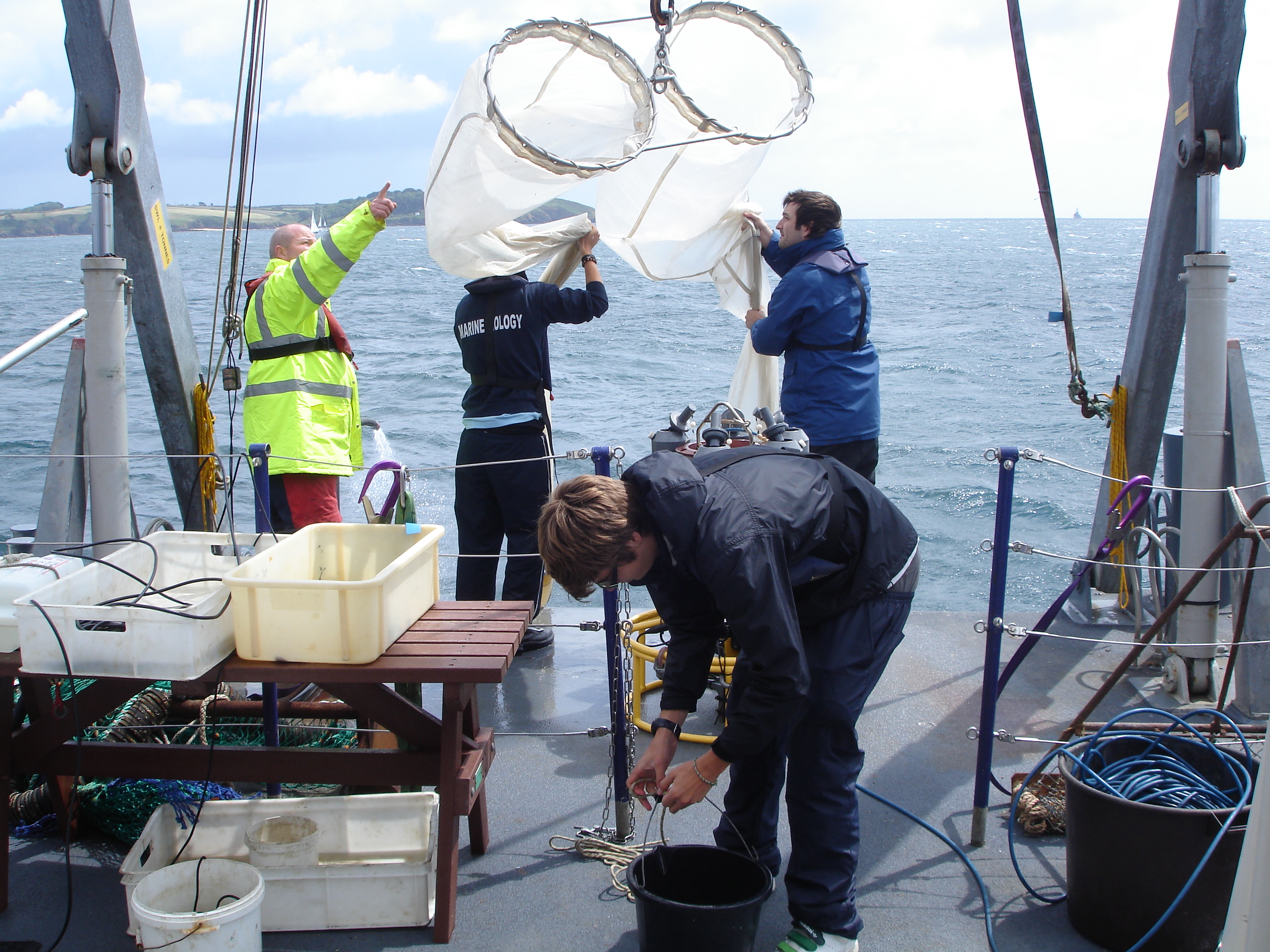 Figure 9.2: Bongo Net Deployment
Figure 9.3: Work in wet lab onboard Callista
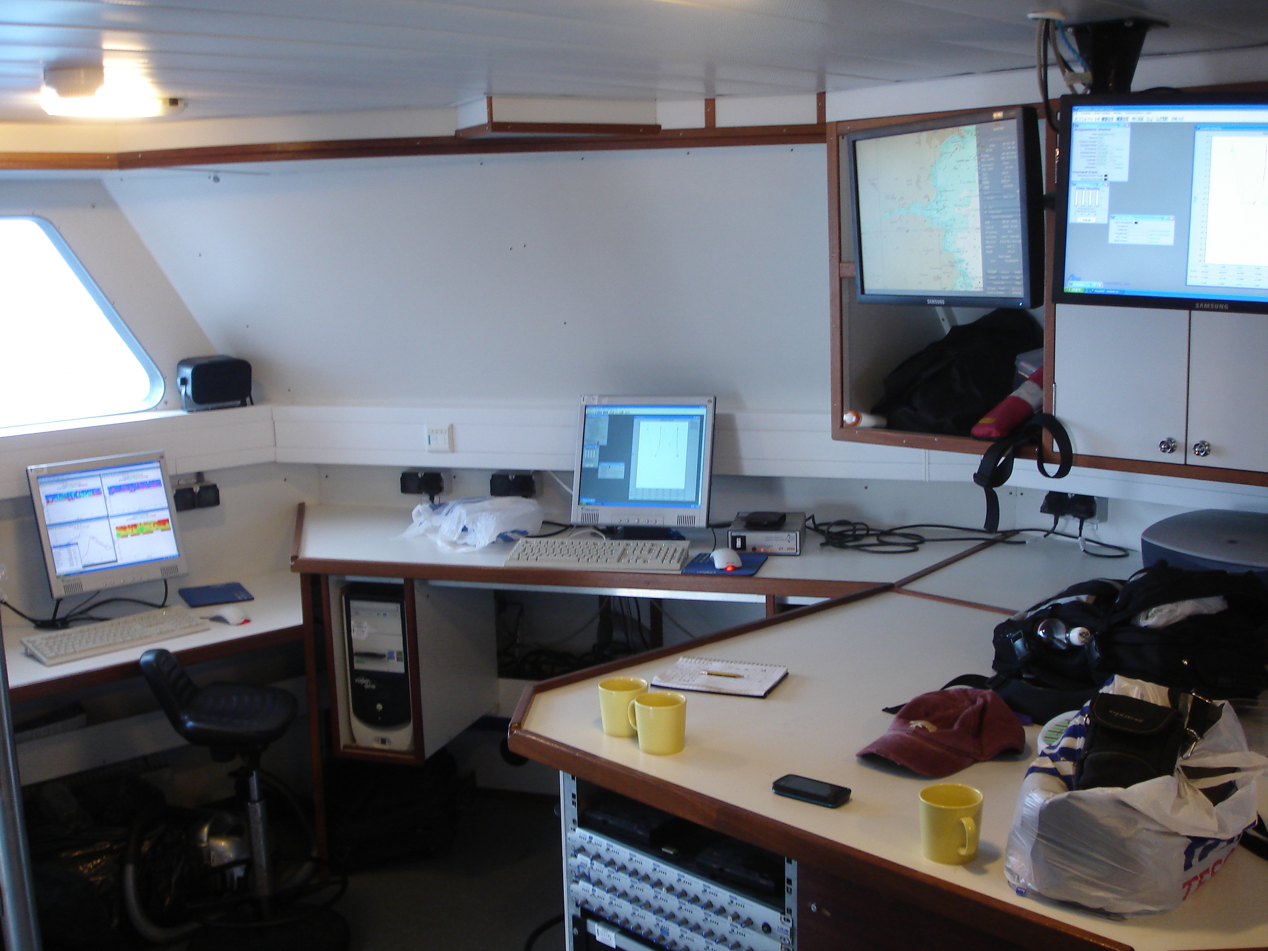
Figure 9.4: The Callista dry lab
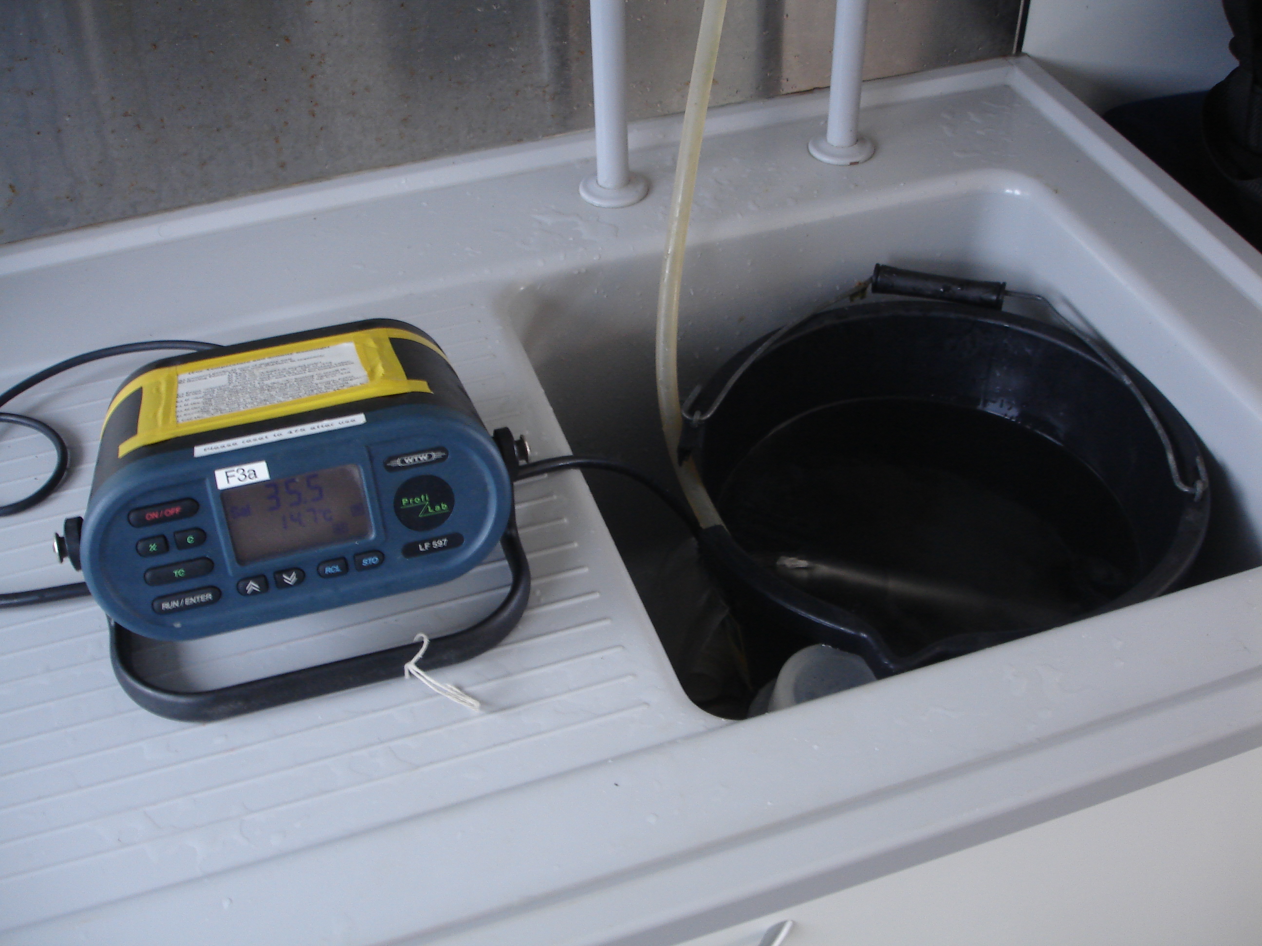
Figure 9.5: Continous measuring of Temperature and Salinity using T/S Probe |
|
NITRATE
Most samples were found to have undetectable nitrates due to the concentration being below the detection limit of the flow injection analyser (0.1µM). This is where the concentration of nitrate in the sample is below or equal to the concentration of nitrate in the reagents. Four samples showed nitrate concentrations above this detection limit however a trend in the data is not evident. No graphs have been used in further analysis. SILICON Little variation in silicon concentration with depth was displayed at each site, however, when all data plotted against depth, there is a clear increase in silicon concentration with depth (figure 10.1). The lowest value of silicon was recorded at station 6 at 30m where a concentration of 0.89 µmol/L was seen. These data were taken during a flooding tide. PHOSPHATE There is an overall increase in phosphate concentration with depth from 0.14µmol/L at 0m depth, to 0.63µmol/L at 16m depth (figure 10.2). Following the same trend as silicon, there are two points at 30m with low phosphate concentrations. DISSOLVED OXYGEN Oxygen saturation can be seen to decrease rapidly at stations 1, 3 and 4 (Figure 10.3). Samples taken from 0-10metres depth at these stations show an average surface saturation value of 101.4%. CTD Casts 2 and 6 were performed at the mouth of the the Helford and Fal rivers respectively. Both sites demonstrate significantly steeper oxygen saturation gradients when compared to the sites discussed above (Figure 10.3). Station 6 shows a decrease of 2.9% between depths of 1.3 and 30 metres with the gradient increasing past 10 metres. The shallower station 2 shows a decrease of 0.7% between surface waters and 7 metres depth. The greatest oxygen saturation can be seen at station 5, taken in the Helford estuary, where surface levels were recorded at 106.7% decreasing by 0.5% down to 4 metres depth.
|
 Figure 10.1: Changes in Si concentration with increasing depth for samples taken on 06/07/2009 between 08:31 and 13:52 GMT from Black Rock to the Mouth of the Helford River.
Figure 10.2: Changes in phosphate concentration with increasing depth for samples taken on 06/07/2009 between 08:31 and 13:52 GMT from Black Rock to the Mouth of the Helford River.
Figure 10.3: Changes in Oxygen saturation with increasing depth for samples taken on 06/07/2009 between 08:31 and 13:52 GMT from Black Rock to the Mouth of the Helford River. |
|
BIOLOGICAL RESULTS |
||
|
PHYTOPLANKTON Stations 2, 3 and 4 show high relative abundance of dinoflagellates to diatoms, with Karinia mikimotoi as the dominant species throughout the water column. Other dinoflagellate species showed increased relative abundance at various stations and depths, such as Titinnina at station 3 (1.3m). Stations 1 and 5 show a less defined dominance trend. Abundances of dinoflagellates and diatoms are relatively equal , with the dominant diatom species being Rhizosolenia at station 1 and Chaetoceros at station 5. Station 6 is the only station that shows a higher relative abundance of diatoms to dinoflagellates, with Chaetoceros again dominant. |
||
|
Figure 11.1: Relative abundance of Diatoms to Dinoflagellates at Stations 1 - 6. Data was collected on 06/07/09 |
Figure 11.2: Number of individuals of Phytoplankton groups/orders at Stations 1 - 6. Data was collected on 06/07/09 |
Figure 11.3: Zooplankton composition present at Stations 2 and 4 using a 100uM and 200uM Bongo plankton net |
|
ZOOPLANKTON Figure 11.3 illustrates the composition of zooplankton present at stations 2 and 4 for both plankton nets. Station 2 was situated in the mouth of Helford River whereas station 4 was in Falmouth Bay. Of the species of zooplankton found in the 100µM sample, station 2 displayed significantly greater abundances than station 4. Hydromedusae were found to be dominant at station 4 with 210 individuals per m3. Conversely, at station 2, Gastropod larvae were found to be dominant with 70 individuals per m3. Other species were present at station 2, predominantly Cirripedia larvae, Hydromedusae and Siphonophors. In addition to hydromedusae, gastropod larvae and copepods are prevalent with numbers of 89 and 57 individuals per m3 respectively. In the 200µm samples, the dominant species in both samples were Hydromedusae, however, at station 2 the difference between Hydromedusae and Siphonophor numbers of individuals are negligible (8 individuals per m3). It must be noted however that the error bars calculated from the standard deviations of the samples at station 4 suggest a large degree of uncertainty with regards to hydromedusae abundance. When compared to the 100µM sample, the diversity within the 200µM sample is higher with species such as Bivalve larvae Echinoderm larvae present.
|
||
|
(click images to enlarge)
Figure 12.1: Velocity Magnitude and Direction for Transect 1 [click here to see ship track]
Figure 12.3: Velocity Magnitude and Direction for Transect 3 [click here to see ship track]
Fig 12.5: Velocity Magnitude and Direction for Transect 5 [click here to see ship track]
Figure 12.6: Longitudinal salinity profile between Helford estuary (station 5) and the estuary mouth (station 2). Blanking files have been applied to remove unreliable data. Vertical columns of stars represent data acquisition points on CTD upcast. NB: from left to right temperature profile goes from offshore to inshore.
Figure 12.8: Longitudinal salinity profile between CTD station 1 (offshore) and Carrick Roads (station 6). Blanking files have been applied to remove unreliable data. Vertical columns of triangles represent data acquisition points on CTD upcast. NB: from left to right temperature profile goes from offshore to inshore.
Figure 12.10: Longitudinal salinity profile between the mouth of the Helford estuary (station 2) and the northern part of Falmouth Bay (stations 3; 4). Blanking files have been applied to remove unreliable data. Vertical columns of triangles represent data acquisition points on CTD upcast.
Figure 12.13: CTD Data from Station 2
12.15: CTD Data from Station 4
Figure 12.17: CTD Data from Station 6 |
ADCP Transect 1 shows no definitive change in flow velocity however the flow direction does show a slight variation at either end of the transect (figure 12.1). This suggests that this slight variation in flow direction is due to estuarine outflow. Transect 2 shows higher surface flow velocities around St Anthony Head decreasing gradually across the mouth of the estuary with the lowest values occurring in the shallower water near Pendennis Point (figure 12.2). The flow direction shows a net flow into the estuary. This is concurrent with the tidal information at the time (flooding tide) and the stick ship track (SST) surface flow directions, however the surface flow velocities shown on the SST contradict the surface flow velocities shown in figure 12.2. The stick ship track shows highest velocities around Pendennis Point whereas the flow velocity figure shows highest velocities at St Anthony Head. Transect 3 shows similar trends in flow velocity and direction as transect 2. Figures 12.2 and 12.3 show flow directions are very similar with a general net flow into the estuary. The SST and velocity magnitude figures for Transect 3 agree with increased flow velocities around Pendennis Point and decreased velocities towards St Anthony Head. This also conforms with the stick ship track for Transect 2. This would suggest that the high flow velocities around St Anthony Head in Figure 12.3 could be small scale random currents caused by the headland. Transect 4 showed similar trends in flow velocity and direction to Transects 2 and 3 with the only noticeable difference being a slight reduction in flow velocity (figure 12.4). This concurs with the tide times as Transect 4 was taken closer to high tide and therefore flow velocities would be slightly lower. Transect 5 displayed maximum flow velocities in the channel with reduced velocities either side (Figure 12.5). The flow direction figure for Transect 5 shows a consistent general direction in the channel, with the directions of flow becoming more random as the distance from the channel increases. This is reinforced by the SST. CTD Longitudinal temperature and salinity contour plots were produced using data acquired by CTD casts 2 (09:31) and 5 (11:40). Data were collected during ebbing tide (LW: 11:01; 1.5m). Data from the two stations are temporally and spatially separated. CTD station 2 was located near the mouth of the Helford estuary, whilst station 5 was located within the main channel of the estuary. Results show that there is a longitudinal temperature (15.7°C to 14.5°C) and salinity (35.20 to 34.7) gradient, but that no vertical gradients can be seen. The Helford River has low freshwater discharge, thus, no halocline was observed at the proximal station (figure 12.6). It should be noted that both CTD casts were made at discrete moments in the tidal cycle, and so, may not provide a true geographical representation of the physical structure of the water column at a given time The indication is: that the transition zone between the Helford estuarine environment and offshore waters is well mixed. This is due to the physical dynamics such as tidal forcing and local geomorphology. Similarly, no vertical thermal structure can be seen (figure 12.7), which is concurrent with the previous conclusions made on the physical dynamics in this transition zone. Longitudinal temperature and salinity plots were made using data acquired by CTD casts 1 (08:31) and 6 (13:52). Data were, therefore, collected 2.5 hours before and 2.5 hours after low tide (LW: 11:01; 1.5m). CTD station 1 was located at Black rock, whilst station 6 was located further north, in Carrick Roads. These data have been presented for completeness, although their relevance as to the true spatial pattern between Carrick Roads and the mouth of the estuary is cast into doubt due to the temporal separation between data acquisitions. A strong thermocline can be observed for station 1 (figure 12.9). A strong halocline can also be observed. Contrarily, data acquired at Carrick Roads, and 5.5 hours after acquisition at Black Rock, indicates a water column which is distinctly well mixed. The evident discontinuity is due to the temporal separation in data acquisition; the tide was ebbing when station 1 data were acquired, and flooding at station 6. Despite the temporal separation in these data, it is possible to make observations as to how the thermal the physical structure changes at the mouth of the estuary, with the tidal cycle. The indication is that offshore waters are stratified, whereas waters in the more dynamic intertidal zone are well mixed. At the time of sampling, the waters at Black Rock were characteristic of an offshore environment. A longitudinal temperature and salinity transect was created, using data from CTD stations 2 (09:31), 3 (10:23) and 4 (10:45). Figure 12.10 is a ‘slice’ from the mouth of the Helford Estuary to N.Falmouth Bay. Due to weather restrictions, it was not possible to perform inshore-offshore transects. Transects run from west to east along the coast where no riverine inputs of freshwater occur. When considering figures 12.10 and 12.11 it is important to note that the graphing programme, Surfer, may have placed isotherms and isohalines inappropriately. The thermal structure of this region does not show any distinct stratification. At station 2, warmer waters were observed close to the surface (~1.3m) than at depth. Similarly, the upper part of the water column, at station 3, is not thermally stratified. Again, station 4 shows little stratification in the upper waters. From station 2 to 4, it is interesting to follow the 14°C isotherm, which is found at 7m; 5.5m; 8m. The salinity structure shows distinct vertical stratification between the CTD cast locations; fresher water is found close to the surface. Salinity is relatively constant throughout the water column at all 6 stations with a value of approximately 35. The exception appears at station 1 which varies from 34.9 to 35.2 at 5m depth (figure 12.). Fluorescence increases with depth down to approximately 6m from 1.4 to 1.9, remains constant at 1.9 to 14m before decreasing again to 1.4 at 16m. Temperature remains constant down approximately 4m before decreasing rapidly to 13.8ºC at 6m. At station 2 there is a gradual decrease in temperature from 14.45ºC at the surface to 14.25ºC a trend which is followed closely by dissolved oxygen (figure 12.). This coincides with a steady increase in fluorescence with depth from 1.35 at 1.5m to 1.85 at 7m. This trend continues at station 3, however the chlorophyll maximum of 2.4 is reached within the thermocline at 9m. The fluorescence maximum observed at the thermocline concurs with the chlorophyll maximum. The highest discrete phosphate (0.625µmol/L) value was also found at 9m, before decreasing markedly to 0.37µmol/L at 14m. Once again the dissolved oxygen follows the temperature trend very closely. Temperature at station 4 remains constant down to 5m before decreasing rapidly to 13.9ºC at 10m. This coincides with a steady increase in fluorescence from 1.4 to 2.0 within the thermocline at 10m. Oxygen once again coincides closely with temperature as in stations 2 and 3. Stations 5 and 6 both show a steady increase in fluorescence with depth coupled with a decrease in temperature and dissolved oxygen. Phosphate and chlorophyll show no outstanding trend with depth. Turbulence at Station 1 increases gradually and linearly with depth from 3.8V at the surface to 5V at 16m. It must be noted that a large amount of noise was recorded at the surface making interpretation difficult. Station 2 shows constant turbidity of 3.9V throughout the water column. Turbulence at Station 3 shows marked variability compared to the previous stations. Initially, turbulence stays constant at 4V from the surface down to 4m then decreases to 3.85V between 4m and 10m before increasing to 4V by 14m. Station 4 shows a gradual decrease in turbulence from 4.03V at the surface to 4.01V at 8m before decreasing more rapidly to 3.88V between 8m and 10m. Turbulence at Station 5 shows a linear decrease from 3.57V at the surface to 3.55V at 4m with the exception being a spike of reduced turbulence at 2m where the transmission drops to 3.53V. Finally turbulence at Station 6 remains relatively constant between the surface and 25m only fluctuating between 4V and 4.02V. It then increases between 25m and 30m from 4.02V to 4.1V. RICHARDSON NUMBER Richardson numbers (Ri) were calculated using CTD and ADCP data. It was not possible to calculate Ri for the upper 3 meters of the water as the ADCP is attached to the hull of R.V. Callista, 1.8m below the surface and the data processing programme, WinRiver, only provides current velocities at 1.5 m intervals through the water column. Ri allows us to ascertain whether mechanical mixing is likely to be occurring. Critical values are plotted on figures 8.7 to 8.11. It is expected that thermally stratified waters will have low Ri values at the surface and close to the seabed where shear causes turbulence. Higher Ri values are expected below or at the thermocline. The formula needed to make this calculation is:
Ri < 0.25 - mixing likely; 0.25 < Ri < 1 - transition zone; Ri > 1 - mixing unlikely At station 1 strong thermal stratification was observed with a 2-3°C thermocline between 6 and 8 m. Above the thermocline, the temperature profile is almost vertical, indicating a well mixed layer; this is confirmed by low Ri values. Higher Ri values close to the thermocline are expected as the density gradient imparts stability to the water column. High Ri values close to the seabed at this station indicate that there was little shear with the seabed and that mixing at the bottom of the water column was limited. Station 2 showed very little thermal stratification. Close to the seabed, where shear stresses act, low Ri values indicate mixing. This is probably due to turbulence associated with tidal flow, as, the CTD cast was made 1.5 hours before low water (LW: 11:01 GMT) at the mouth of the Helford River. The temperature profile for Station 3 indicates a slightly stratified water column. An anomalous peak at 10 m is due to interrupting the CTD cast in order to take water samples. Ri values indicate a well mixed water column from 4 m to the seabed. These data were acquired in Falmouth Bay half an hour before low water. Station 3 was located away from any rivers or estuaries, and so, the indication is that local geomorphology combined with tidal flow caused mechanical mixing. It would be of interest to conduct further studies in this region to investigate the residual currents and dynamics of Falmouth Bay. The thermal structure at station 4 indicates a partially mixed water column. Low Ri values between 3 and 5 m, coupled with a homogenous temperature gradient indicate a mixed layer at the surface. As expected, higher Ri values have been calculated where the temperature gradient was strongest. These data were acquired 15 minutes before low water, and so, shear at the seabed was minimal due to slack water. Ri values are therefore low at the sediment-water interface. At Station 6, the thermal structure of the water column, coupled with the Ri values, indicate a well mixed water column for almost its entire depth (30 m). Some anomalously high Ri values were calculated, but the general indication is that mixing was occurring when these data were acquired. This CTD cast was made almost three hours after low water. The flooding tide, therefore, is the cause for this mixing through the entire depth of the water column.
|
(click to enlarge)
Figure 12.2: Velocity Magnitude and Direction for Transect 2 [click here to see ship track]
Figure 12.4: Velocity Magnitude and Direction for Transect 4 [click here to see ship track]
Figure 12.7: Longitudinal temperature profile between Helford estuary (station 5) and the estuary mouth (station 2). Blanking files have been applied to remove unreliable data. Vertical columns of triangles represent data acquisition points on CTD upcast. NB: from left to right temperature profile goes from offshore to inshore.
Figure 12.9: Longitudinal temperature profile between CTD station 1 (offshore) and Carrick Roads (station 6). Blanking files have been applied to remove unreliable data. Vertical columns of triangles represent data acquisition points on CTD upcast. NB: from left to right temperature profile goes from offshore to inshore.
Figure 12.11: temperature profile between the mouth of the Helford estuary (station 2) and the northern part of Falmouth Bay (stations 3; 4). Blanking files have been applied to remove unreliable data. Vertical columns of triangles represent data acquisition points on CTD upcast.
Figure 12.12: CTD Data from Station 1
Figure 12.14: CTD Data from Station 3
Figure 12.16: CTD Data from Station 5 [click here to see 3 day composite MODIS image of surface chlorophyll product (04 to 06-07-09)] |
|
DISCUSSION |
|
Data collected offshore were significantly dissimilar to those collected in the proximal part of the Fal Estuary. Poor weather conditions meant that it was not possible to perform a longitudinal transect from estuary mouth, through the thermal front, and into the ‘true’ offshore region. It has already been shown that Nitrate and Silicate concentrations decrease towards the distal part of the estuary, the same is also true concerning phytoplankton and zooplankton abundance. Offshore, nitrate concentrations were either very low or outside the detection limits of the flow injection analyser; this is due to their non-conservative nature as essential nutrients for marine autotrophes. Phosphate and Silicate concentrations were detectable, but Nitrate remains the proximally limiting nutrient for primary production. Data from the L4 buoy (www.westernchannelobservatory.org.uk) for the beginning of July, show concentrations ranging from 0.04 to 0.56 µM.l-1 for phosphate; 0.05 to 0.94 µM.l-1 for Nitrate and Nitrite; 0.12 to 3.89 µM.l-1 for silicate (2000 – 2008). Our results agree, therefore, with the ranges recorded offshore of Plymouth, to the West of Falmouth and allow us to have confidence in the quality of our data. Residence time calculations indicate that although nutrients are concentrated in the proximal part of the Fal system, low riverine discharge means that it would take 30 days for the volume of the estuary to be replaced by freshwater. During the spring bloom and summer months, nutrient flux slow and is utilized prior to arrival in the offshore environment. Surface O2 saturation was consistently lower than values recorded in the Fal Estuary, particularly in the proximal region. This is linked to the limited autotrophic productivity when compared to the estuarine environment. The biological structure of the offshore environment was, again, dissimilar to that of the estuarine region. Physical results show that, on the whole, the Fal estuary is partially to well mixed, with the exception of the upper reaches (River Fal) where there is a vertical density gradient. Offshore, thermally stratification was observed, in particular at Black Rock. At all other CTD locations, the water column was well mixed, with the exception of Falmouth Bay, which was partially mixed. This has consequences for the structure of the biota. Richardson Number calculations and longitudinal contour plots of density and temperature confirm these ascertains. It is evident that tidal flow induces shear at the seabed (ADCP and Ri data), re-suspending non-cohesive sediment in the estuarine regions (transmission data combined with Ri calculations and ADCP). This will have consequences for the bedforms that will be observed during the Geophysical survey. The low phytoplankton abundance results indicate that the spring bloom of diatoms ended long before the beginning of sampling. This is typically followed by a late summer bloom of dinoflagellates once the surface waters have reached highs in temperature causing stratification. Nutrient concentrations have also had time to recover through remineralisation of the thermocline. Although the physical conditions may exist for dinoflagellate blooms the nutrient concentration remains limiting. Data from L4 show that offshore nutrient levels prior to the spring bloom (09-03-09) were: silicate – 3.77 µM.l-1; nitrate and nitrite – 6.67 µM.l-1; phosphate – 0.45 µM.l-1. This supports the argument that the spring bloom of diatoms has already occurred. It would be of interest to conduct further sampling in several weeks to investigate the decline of the zooplankton.
|
![]()
![]()
![]()
![]()
![]()
![]()
![]()
![]()
![]()
|
Date: 09/07/2009 [click for tidal data] Cloud Cover: 4/8; Rain: none; Wind: Gusting to 2 |
|
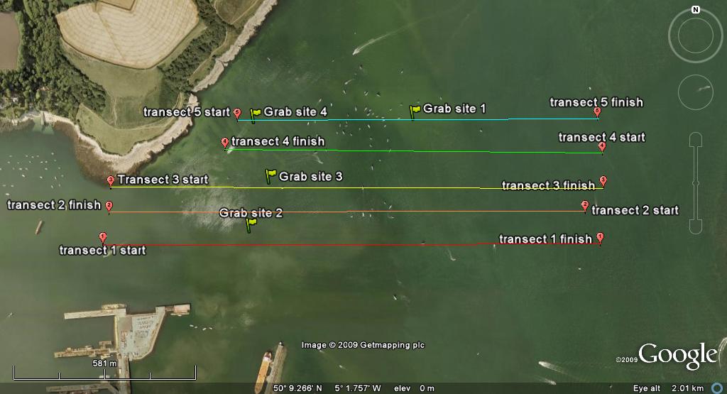
| Data was collected on 09/07/2009 from the Fal Estuary outer harbour to Carrick Roads channel using geoacoustic 415khz side scan transects, an underwater video camera and a Van Veen grab. Surveying commenced at 08:05 GMT and terminated at 09:02 GMT between 050°09.519N, 005°03.432W and 050°09.7354N, 005°09.7354W (for full transect details see Google Earth Image). The principle aim of the survey was to investigate the spatial variability of sediment and biota within this area and determine the benthic habitats present. | |
|
FIELD METHODS
[Figure 13.1: Google Earth Map showing Geophysics boat transects] The geophysical survey was conducted on 09/07/2009 from the Fal Estuary outer harbour to Carrick Roads channel using a geoacoustic 415khz side scan sonar, an underwater video camera and a Van Veen grab. Surveying commenced at 08:05 GMT and terminated at 09:02 GMT between 050°09.519N, 005°03.432W and 050°09.7354N, 005°09.7354W (click here for full transect details). Data were collected using the side scan sonar which was towed at approximately 4 knots to ensure maximum resolution. Grab sites for the Van Veen grab were determined using the underwater camera to avoid disturbing live mearl beds. The samples were then analysed on deck for sediment grain size and local biota special diversity. The principle aim of the survey was to investigate the spatial variability of sediment and biota within this area and determine the benthic habitats present. The sidescan sonar was towed behind the vessel along each transect line. Printouts from the sidescan were used to find areas of interest for Van Veen grabs to be taken. A video camera was used at each grab site to ensure samples of live Maerl were not taken and the grab to be a good representative of the surrounding seafloor. The contents of the grabs were analysed in relation to the type of sediment (abiotic factors) and identification of living fauna (biotic factors) using identification keys and 2mm and 1mm mesh sieves. Unidentified fauna were photographed with a scale for further identification in the lab.
|
|
|
GRAB 1 -
0930 GMT, 050°09.7340 N;
005°02.5930 W, Depth of
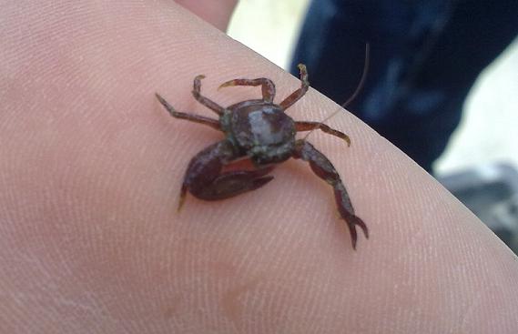
Water Column – 9.0 metres Sediment The grab consisted of approximately 35% coarse sediment, 25% dead Maerl and 30% dead bivalve shells. Biota Approximately 5% of the grab sample was red/brown macroalgae (Rhodymenia pseudopalmata). Other species present were 1 Hermit Crab, 2 Common Spider Crabs (Maja squinado), 1 Ascidian, 1 Bivalve (Tapes ssp.) and 1 Moon snail (Polinices catenus).
|
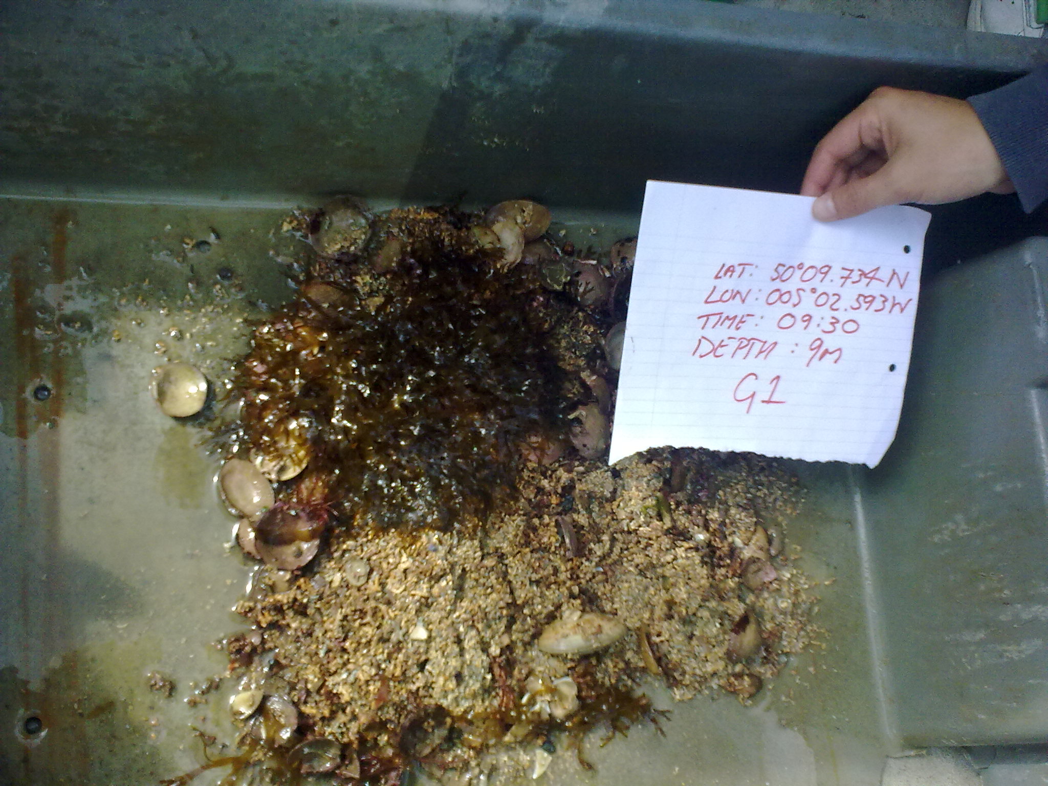 [Figure 13.2: Contents of Grab Sample 1 including red/brown macroalgae (Rhodymenia pseudopalmata)] |
|
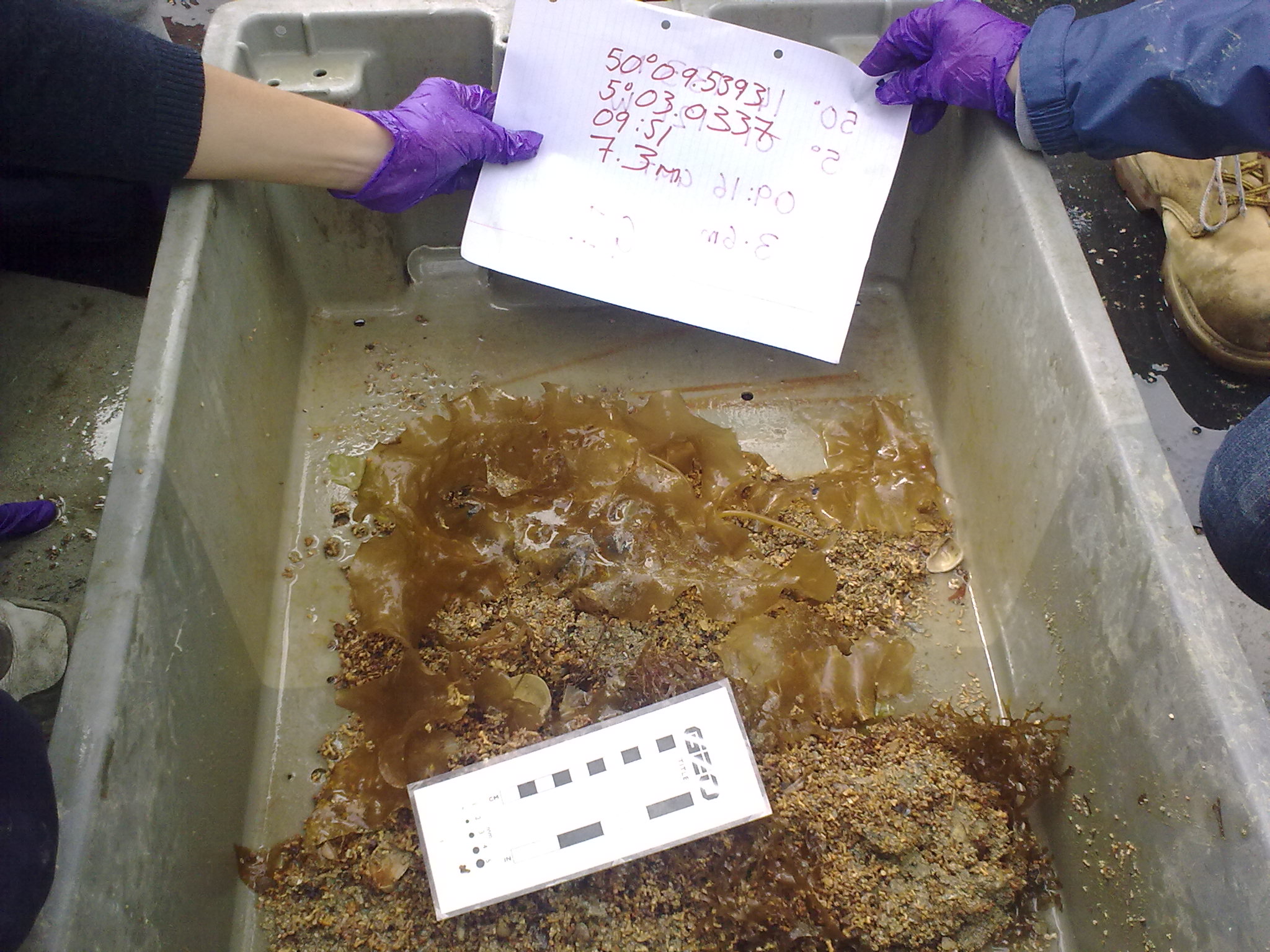
GRAB 2 -
0951 GMT, 050°09.5392 N; 005°03.0337 W,
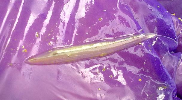
Depth of Water Column – 7.3 metres Sediment In contrast to grab 1, the sediment consisted of 50% dead Maerl and contained less coarse sediment (approximately 15% of the total sample). Similarly to grab 1, there were about 20% dead bivalve shells. Biota Organisms found were an Amphioxus, 2 polychaetes, a Grey topshell (Gibbula cineraria) and a Decapod crab (Xantho poressa). 10% of the sample was composed of brown macroalgae (Dictyopteris membranacea), which used a dead bivalve shell as biogenic substratum
|
[Figure 13.3: Contents of grab site 2 including a scale and brown macroalgae (Dictyopteris membranacea)]
|
|
GRAB 3 -
1010 GMT, 050°09.6242 N; 005°02.9802 W, Depth of the Water Column – 7.3
metres
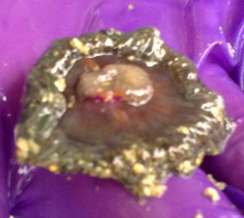
Similarly to grab site 2, dead Maerl was the main component of the sediment. Less dead bivalve shells were found (approximately 10%) and the sediment appeared to be finer than all other grab sites. Some evidence of anthropogenic influences as a piece of glass was found. Biota A hermit crab, two large polychaete tubes and an anemone (unidentified anthozoan) were found at this grab site. The amount of macroalgae (Dictyopteris membranacea and Furcellaria lumbricalis) present decreased at this site to 5%.
|
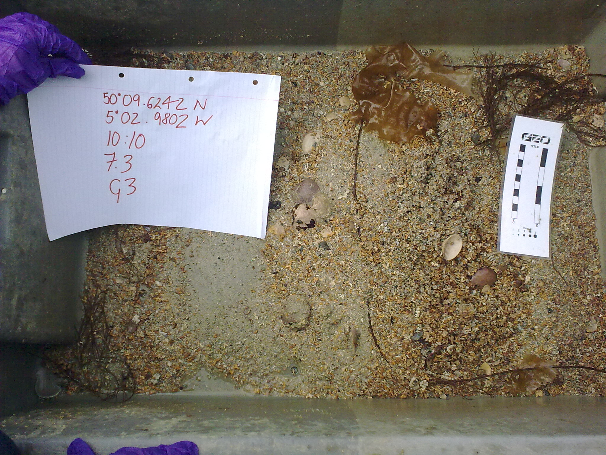 [Figure 13.4: Contents of Grab site 3 including the brown macroalage Dictyopteris membranacea and Furcellaria lumbricalis] |
|
GRAB
4 - 1027 GMT, 050°09.7378 N; 005°03.0214 W, Depth of the Water
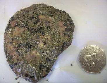
Column – 7.0 metres Sediment This site contained the most (65%) of dead Maerl and the sediment also appeared coarser than grab site 3. Only 5% of dead bivalve shells were found at this site including a common Oyster shell (Ostrea edulis). Biota Grab site four contained the least amount of living organisms with only one Amphioxus and a Ragworm present.
|
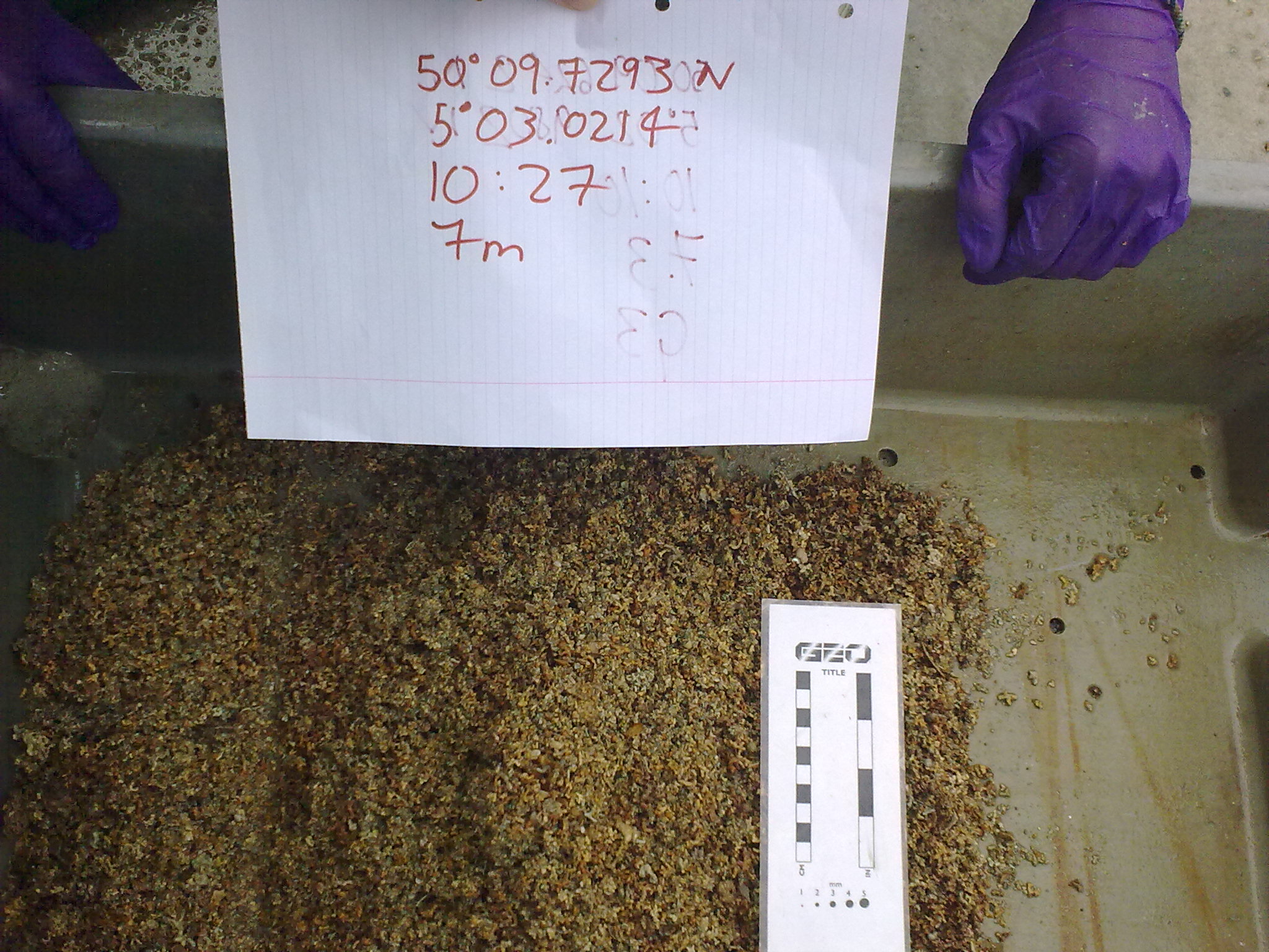 [Figure 13.5: Contents of Grab sample 4.] |
|
The track suggests coarser bottom sediment within the channel, however this is contradicted by admiralty charts which show gravel and shells within the harbour area, and sandy sediment in the channel. Features such as those seen on the side scan trace are nevertheless also found on the admiralty charts: · The anchor drag marks observed on the side scan trace are assumed by Google earth images which show transects 2 and 3 to be surrounded by anchored vessels. The anchor scour marks have been measured at between 0.6 and 0.78m, therefore suggesting that vessels such as relatively large pleasure craft have anchored. · The large area of Bedrock observed from the end point of transect 2 to the start of transect 3 is extended from Trefusis Point, which can once again be confirmed using Google Earth images. · A dense bed of weed was recognized by side scan data between transects 4 and 5. This was confirmed by admiralty chart data, which shows presence of ‘weed’ at this site, along with video data allowing identification as Palmaria palmata. |
|
|
· Site 1 contained the greatest biodiversity as it is located closer to the Carrick Roads Channel, which has a higher flow velocity. This benefits suspension feeders such as Ascidians and bivalves due to increased food availability. No physical bedforms were recognised at sites 2 and 3, therefore there was little variation in the biology observed. Site 4 had the lowest faunal and floral diversity, which may have been a function of a Palmaria palmate bed out-competing other organisms for sunlight and nutrients. Dead mearl was observed at all sites, and represents the calcareous algae stated on admiralty charts.
|
|
|
NITRATE The flow injection analysis method was employed for nitrate analysis in the lab. This method involves the use of a peristaltic pump, and an injection valve with a flow through detector. See Johnson and Petty (1983) for further information on this method. SILICON Silicon concentrations were calculated with the aid of a U-1800 spectrophotometer. See Parsons et al (1984) for further information however it must be noted that the molybdate reagent was used at the following ratio - Metol Sulphite : Oxalic Acid : Sulphuric Acid : Water - 10 : 6 : 6 : 8 PHOSPHATE The phosphate was analysed as per Parsons et al. (1984). The standards used were 0.15, 0.30, 0.75, 1.5 and 3.0 µmol l-1. The samples, standards and blanks were analysed using a using a U-1800 Spectrometer with a cell size of 4cm. DISSOLVED OXYGEN The dissolved oxygen was analysed using the Winkler method involving introduction of the reagents: Manganese chloride and Alkaline iodide to water samples. See Grasshoff (1999) for further information. CHLOROPHYLL 50 ml samples of seawater were filtered through a glass fibre filter (GFF) then placed in plastic tubes containing 6ml of acetone. Fluorescence was measured using a 10AU Fluorometer as per Parsons et al (1984). PHYTOPLANKTON Taxonomy Analysis Method A seawater sample of 100 ml was collected from a specific depth (surface) and placed in a glass bottle. It was fixed and stained using lugols iodine and was chilled. Samples were placed in a measuring cylinder to allow the phytoplankton to settle out. Excess fluid was removed using a vacuum pump with an inverted glass pipette. The sample was stirred to re-suspend and allow a representative sample. A 1ml of sample was analysed under Motic SMZ-168 light microscopes. Species were counted in 5 columns in a Sedgewick Rafter chamber, further calculation was undertaken on the numbers of phytoplankton per litre. ZOOPLANKTON Taxonomy Analysis Method Zooplankton were obtained using plankton nets. Distance was recorded using an impellor, which was used to calculate the volume of water and from this the abundance of zooplankton can be recorded. Zooplankton was fixed using 20 ml of 10% 2ml of samples were placed in a Bogorov viewing chamber and groups were identified under 50x identification.
|
![]()
| Parsons T. R. Maita Y. and Lalli C. (1984) “ A manual of chemical and biological methods for seawater analysis” 173 p. Pergamon Grasshoff, K., K. Kremling, and M. Ehrhardt. (1999). Methods of seawater analysis. 3rd ed. Wiley-VCH. Johnson K. and Petty R.L.(1983) “Determination of nitrate and nitrite in seawater by flow injection analysis”. Limnology and Oceanography 28 1260-1266.
|
|
DISCLAIMER |
|
The opinions and views expressed on this website do not represent those of the University of Southampton or the National Oceanography Centre.
|


![[Click for Tidal Data]](tideb.gif)
![[click here to see ship track]](traka.GIF)
![[click here to see ship track]](trakc.GIF)
![[click here to see ship track]](trake.GIF)
![[click here to see ship track]](trakb.GIF)
![[click here to see ship track]](trakd.GIF)
![[click here to see 3 day composite MODIS image of surface chlorophyll product (04 to 06-07-09)]](modis.JPG)
![[click for tidal data]](tidegeo.GIF)