Falmouth - Group 8 2009

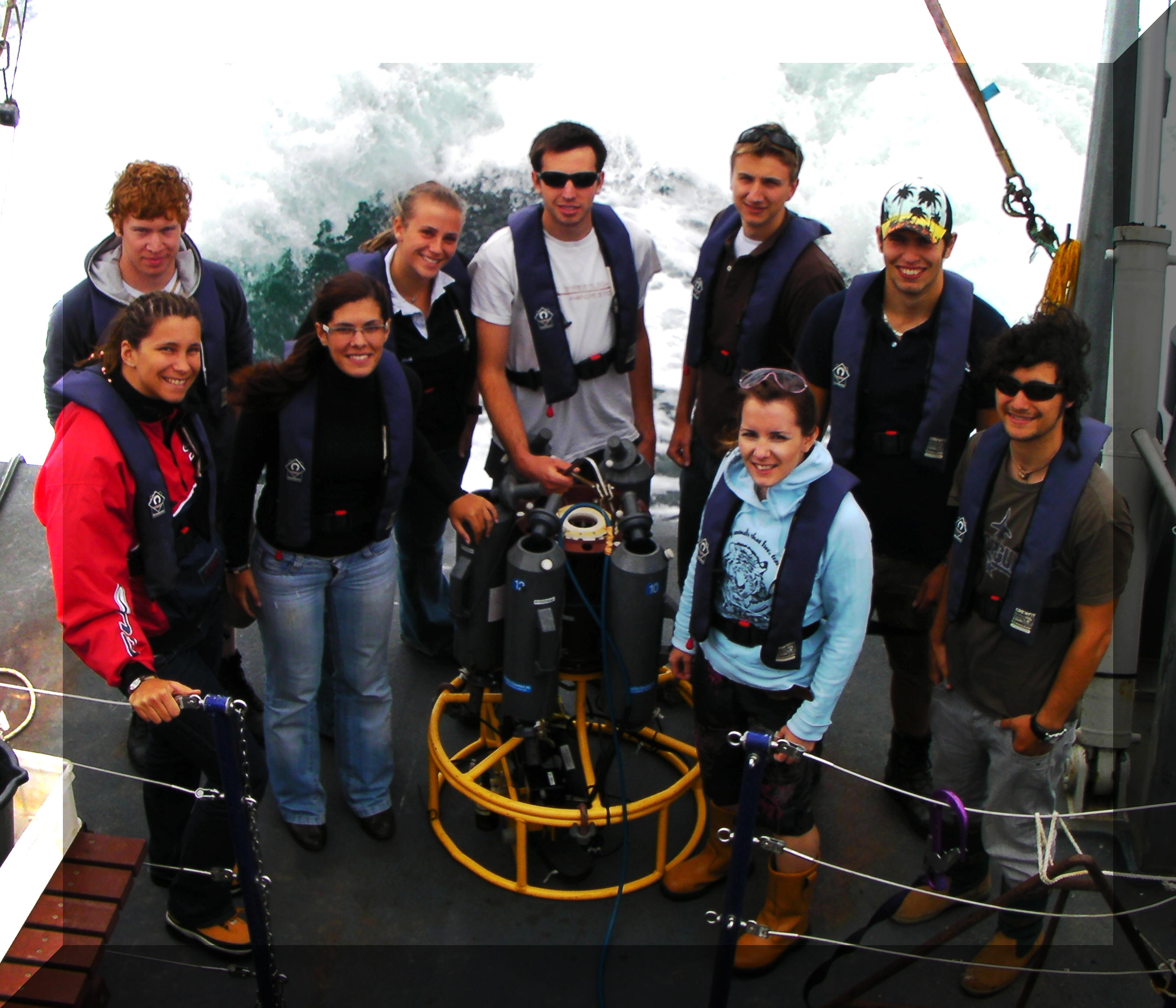
Joana Almeida, Aaron Cooper, Jamie Harding, Gideon Mordecai, Giulia Mussap, Emily Parsons, James Ranson, Ross Taylor, Jenny Thompson   

Introduction

Introduction

The Fal estuary is situated in Falmouth, Cornwall on the south west coast of England. The Fal is a ria: drowned river valley formed after the last glaciation. Due to an inundation exceeding sedimentation, the estuary has maintained the original topography of the river and valley, and hence is one of the largest natural harbours in the world. The Fal has a large drainage basin being fed by 6 tributaries and many creeks produced in the flooding, despite this there is a low riverine input and it is a seawater dominated estuary with the salinity structure symptomatic of a partially mixed estuary. It is a macro tidal estuary with mean tidal range of 5m at spring and 4.1 m at neap, in the upper regions of the estuary it becomes mesotidal, its max tidal current doesn’t exceed 2 knots.

For the last two centuries the Falmouth area has been dominated by the mining industry making it one of the most metal polluted areas in the UK. This has caused the build up among others of mined materials Copper, Lead, Arsenic and China Clay. As well as mining discharge another point source is discharge from the sewage treatment works. The mining discharge leads to the precipitation of ochres from iron oxides and hydroxides. There is also the recent impact of Wheal Jane incident (January 1992) at Restronguet creek when toxic elements were released into the Carnon river. The long term effects of this are the remobilisation of metals from the sediment over time which led to the establishment of a high density sludge.

Due to the extensive pollution from mining discharge and diffuse sources such as agricultural runoff, the Falmouth estuary has been chosen as a candidate Special Area of Conservation (cSAC) especially due to the eelgrass, mudflats and maerl beds. As well as this the Fal estuaries have been designated a Sensitive Area under the nitrate directives due to hypernitrification (in the past this has caused toxic algal blooms, the first red tide was observed in 1995). These both aim to reduce nutrient enrichment in the area and improve the water quality.

Our aim in Falmouth is to investigate the biological, chemical, geophysical and physical processes, interactions and contributions in and to the estuarine environment using a variety of equipment and methods.

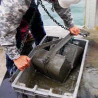
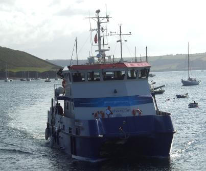
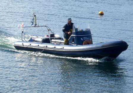
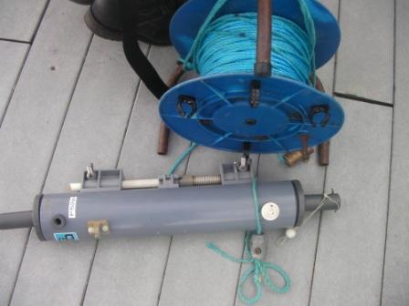
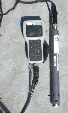
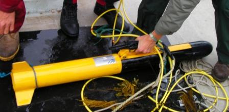
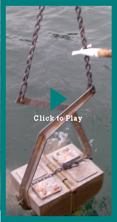
Equipment and Vessels

Geophysics

Introduction 

On Thursday 2nd July 2009, a geophysical survey of the Helford estuary, Cornwall was carried out. The aim of this survey was to analyse the geophysical properties of the estuary, such as the sea bed formations and composition, evidence of anthropological impact on the sea floor, and floral and faunal diversity of the area. It was requested by Natural England that this particular area was surveyed as one year ago, students identified maerl within the estuary, however due to lack of precise logging, the evidence is questionable.

Maerl is a term used to describe several species of calcified red seaweed which can accumulate on the seabed over a long period of time; it is an important habitat for a number of species, as well as being rare. The independent public body Natural England is very concerned with this issue and wanted to know if last year’s findings and identifications were real.

A sidescan sonar survey consisting of 6 tracks was carried out to investigate the bathymetry of the Helford estuary. At 4 different sites in the estuary sediment grabs using a Van Veen grab were taken. Sea floor videos were taken to investigate the sediment type as well as the organisms present before grabs, and to view other interesting features.

Date: 02/07/09
Vessel: RV Xplorer
Skipper: Robin

Crew: Mike
Demonstrator: John Davis
PSO: Emily Parsons
Area surveyed: Helford estuary
Weather:
Conditions were very poor, with heavy rain and temperatures of around 16°C. Wind was mainly easterly and blowing at speeds varying 2 and 12mph. cold front. Visibility was moderate.  

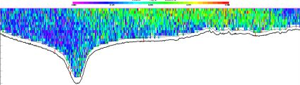
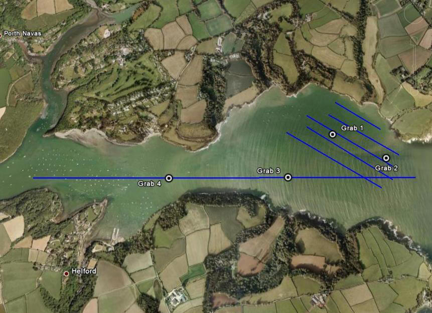
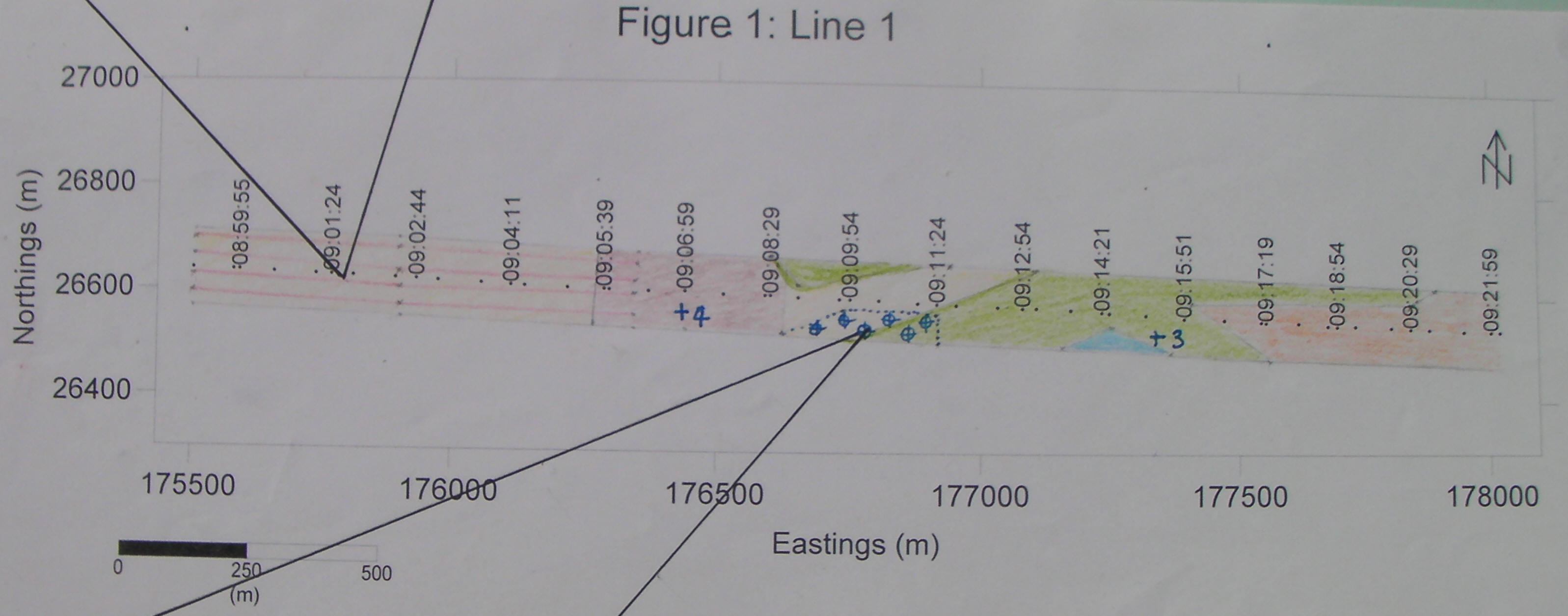
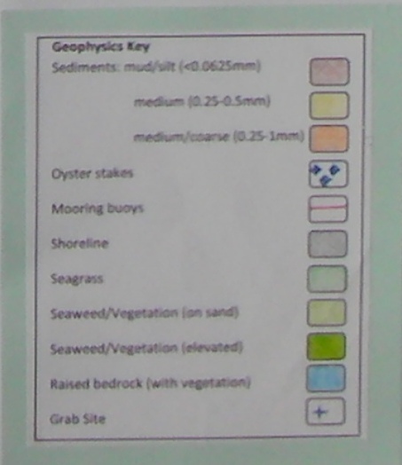
Figure 1. This modified 'Google Earth' image shows the sidescan tracks and grab sample locations within the Helford estuary

The sidescan trace demonstrated that all tracks had sediments ranging from mud and biogenic substrate to coarse sands (0.0625 – 1.0 mm). Differences between the sediment types were indicated by the strength of backscatter for example coarse sediment caused a low return which appeared grainy on the trace. Conversely finer sediments such as mud generated a higher return appearing darker due to less scattering. This data was then interpreted into the figures below using trigonometric calculations to define distance of features from the towfish and their relief.

From the start of Track 1 up to 117000, 26650 (Figure 2) was comprised of medium sand or mud shown by differing contrast in backscatter. This was interspersed with regions of seaweed on top of sand and some anthropogenic feature such as mooring buoys and oyster stacks. The remainder of Track 1 was comprised of seaweed on top of sand with areas of medium/coarse sand.

Figure 2

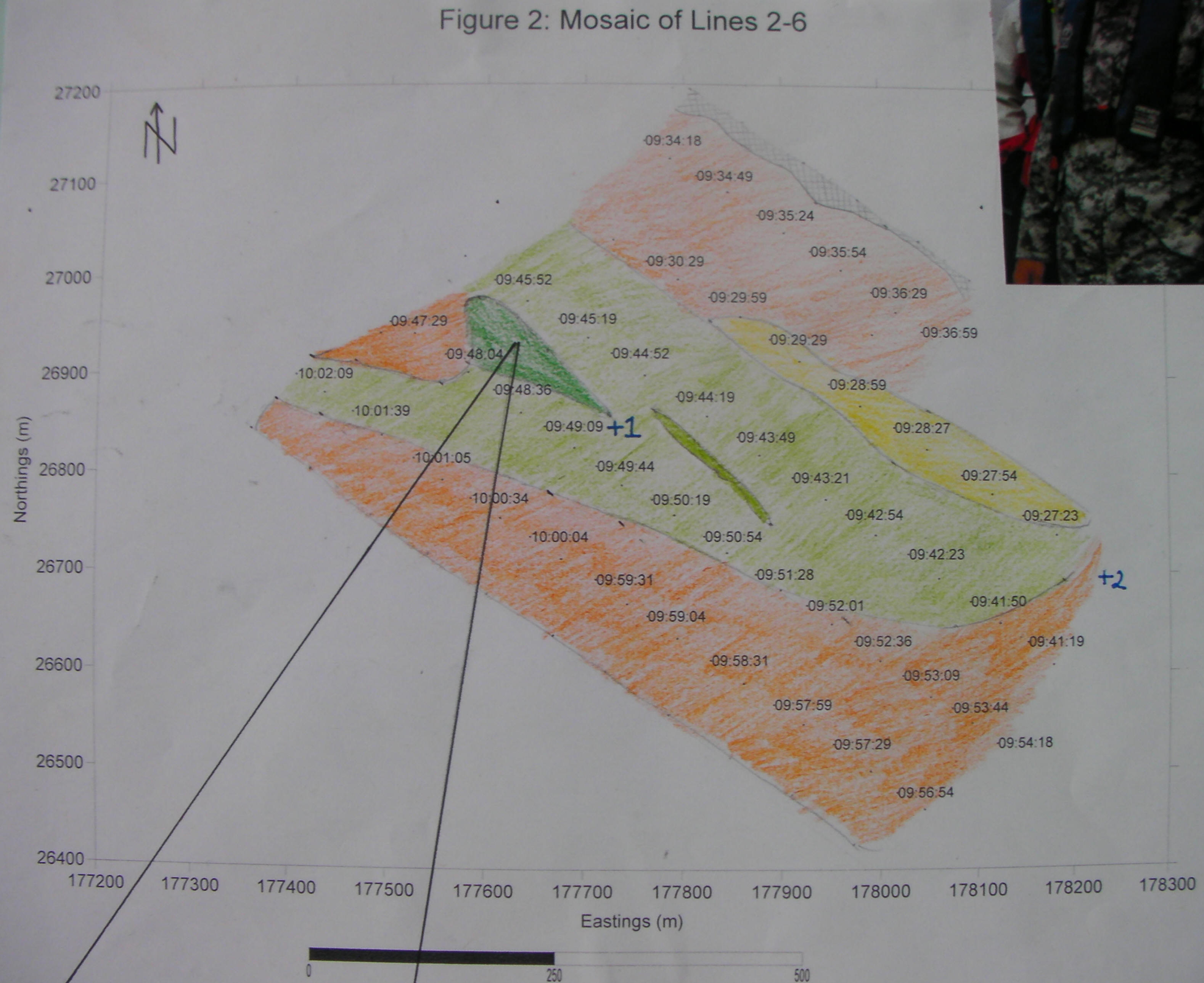
The second region of Tracks 2 -6 (Figure 3) formed a mosaic typified by medium/coarse sands with a central area of vegetation covering the sediment below. The lower boundary of the vegetation is very distinct and is supported by the Google Earth satellite images. On the northern edge of the mosaic, (177900, 27075), the rocky shore line can be seen from the strong elevated return.

Figure 3

The following features on the trace were of particular interest :

The small craft moorings of Helford Point are shown by a characteristic high backscatter. These have no shadow as they were on the water surface not the seabed. This can be caused by sound reflecting off the seafloor, then off the hulls or sound from the sidescan sonar reflecting directly off the hull (figure 4).

Figure 4

On this section of the trace a strong speckled return is symptomatic of macro fauna, such as seaweed, seagrass and Eelgrass (as noted on Admiralty charts of the area). This is due to the reflection from the vegetation perpendicular blades within the water column, however this often masks the underling sediments (Figure 5).

Figure 5

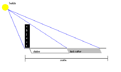
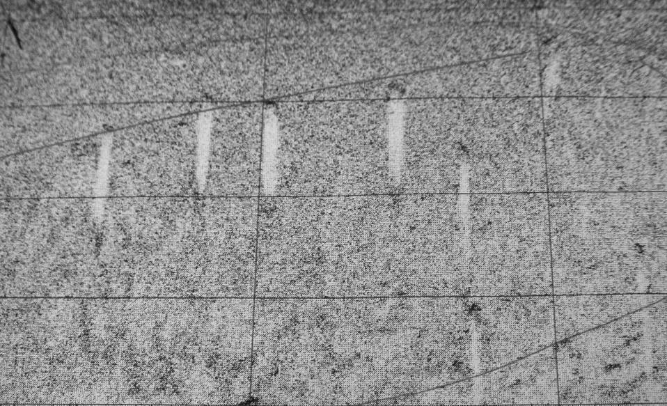
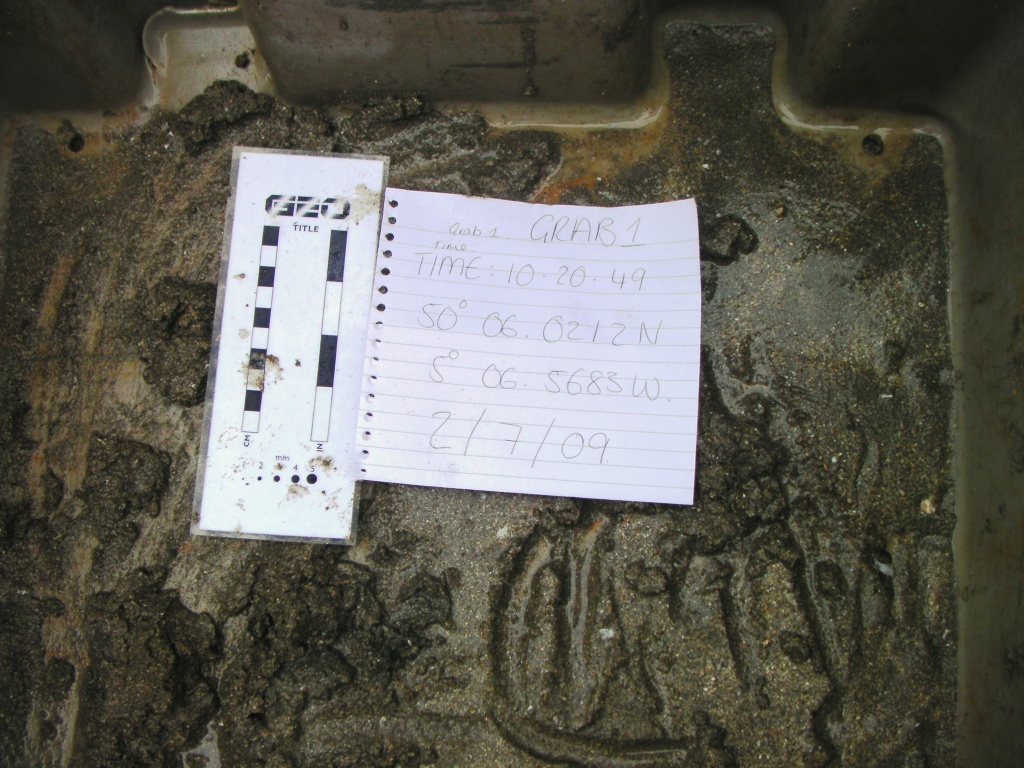
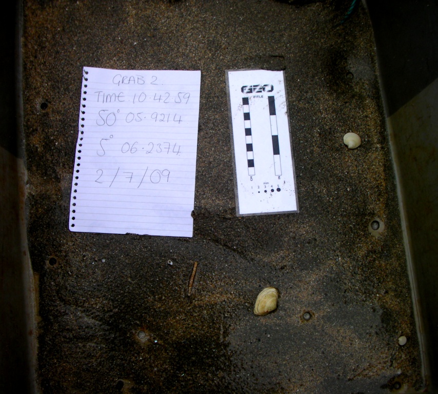
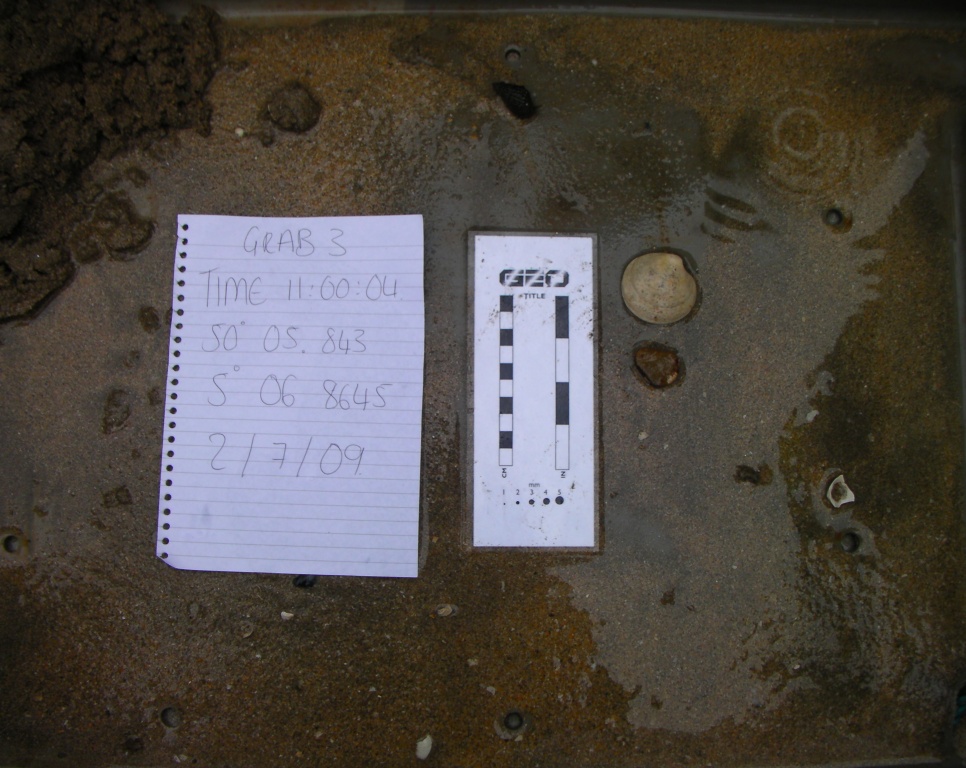
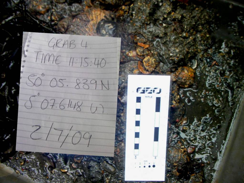
The features below (figure 7) show a large return followed by long shadow which indicates positive relief as indicated by the diagram below (Figure 6). Calculations show the features were between 0.54 - 1.76m above sea floor. When surveying the area many buoys on the surface were observed which are likely to coincide with each individual feature, there was also a fishing trawler collecting pots of some kind, as noted in the log book. Admiralty charts of this region display several areas of oyster farming it can therefore be deduced that these are likely to be oyster pots or similar (Figure 7).

Figure 6               Figure 7

Further Investigation of Site

Having recovered the towfish safely and put it to one side the sonograph was unrolled section by section to pick out possible areas of interest for a grab. Taking grabs of seagrass habitats is prohibited so we could only use the video feed to ascertain it's presence. Once an area was chosen from looking at the trace a video camera was lowered over the starboard side with a weight attached to prevent it moving with the incoming tide too much with some layback being inevitable. This video was always recorded for later ananlysis and 'screen grabs'. From the feed we were able to select a specific grab site. This was repeated for each grab site.

1/2. Sites 1 and 2 were chosen to confirm the boundary seen between the two substrate types, this boundary was also confirmed by the Google Earth image. The video feed for both sites showed similar species and substrate types, confirming the sidescan trace. Maerl was claimed to be found in this area last year so these grabs could possibly have collected some.

3. Site 3 was chosen as the substrate type appeared to change leading up to the pool so a grab was taken as an intermediary. The video feed here showed a slightly higher biodiversity with more biogenic shells.

4. Site 4 was chosen at The Pool as it is much deeper than the surrounding area and the sidescan trace showed a distinctively different substrate type with a much higher biodiversity seen on the video feed.

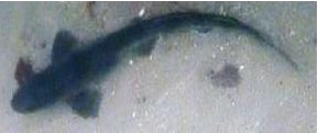
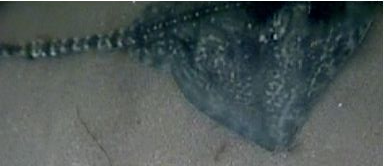
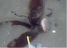
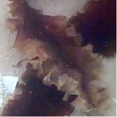
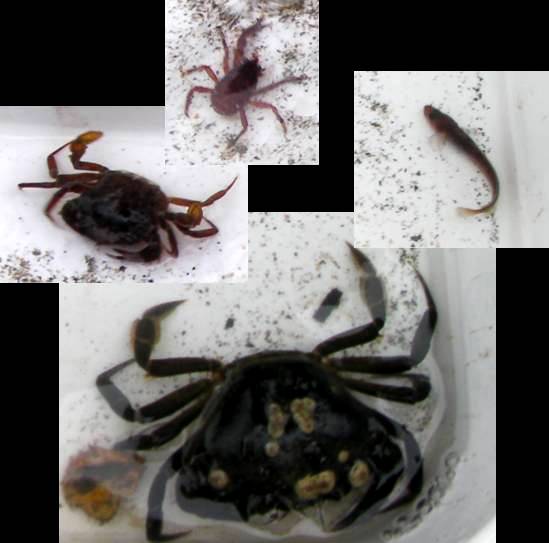
 Video  

Figure 8	Figure 9

Figure 10	Figure 11	Figure 12

An underwater video camera was used to determine the habitat that the grab sample was to be carried out in. This was to primarily prevent a grab sample being done in a sea grass habitat, however, the video footage also gave a unique perspective to the flora and fauna living in the Helford estuary.

At the site of the second grab (figure 1) two elasmobranch species were viewed on the video footage. A 'skate' (Figure 9) was identified as Raja batis which was found living on the sandy sediment. An unidentified species of dogfish (see figure 8) was also seen at the second grab site. The presence of these two top predators in just one short video sweep shows that the Helford estuary is a relatively stable and clean habitat. Perhaps many times less polluted than the adjacent Falmouth estuary where much more industry is situated.

At sites one to three, lots of macro algae were seen. The macro algae was quite sparse, found every few metres. There were several different types of algae seen. Different species of red, green and brown macroalgae were seen (figures 10 and 11) a scallop (bivalve mollusc) can also be seen living on the sandy sediment (Figure 10).

The fourth grab site in 'the pool' had a much higher species diversity. Figure 12 shows an unidentified species of a starfish (echinoderm, asteroidea). Many starfish were seen at this site, probably feeding on the many bivalve molluscs seen at this site        

Conclusion

The oceanographic survey performed on the Helford estuary, yielded a variation of sediment types and consequent variation in habitats at different sites within the estuary. Most specie abundance and diversity was found in the deeper areas, possibly due to the higher current flow down-welling nutrients into the 'pool'. Although no maerl was located, the sidescan trace seems to have located patches of seagrass as well as yielding the anthropogenic influence on the estuary which limits and threatens such populations.

Introduction

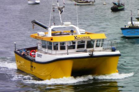
On Monday 6th July 2009, a survey of the Fal estuary was carried out. The aim of the survey was to analyse the biological, chemical and physical variations down the estuary. Half the group starting in the RIB at the Prince of Wales pier proceeded to travel up river on the outgoing tide to get a sample as high as possible up the Truro River before low tide at 11:01GMT. Starting at Malpas Point, 50.14.693N 05.01.369W, the RIB proceeded South taking samples of surface water using a hand held go-flo bottle for nitrogen, phosphate, silicon, oxygen and chlorophyll analysis with phytoplankton and zooplankton samples collected at chosen stations and YSI vertical water column profiles taken at each station as far as the pontoon just before Turnaware Point at 50.12.56N 05.01.675W. The group on the pontoon took a short time series data set from the North edge of the pontoon at point 50.12.971N 05.01.660W sampling the same parameters at 1 and 3 metre depths as well as the vertical YSI profiles.

Having completed the riverine sampling section of the estuary, it was necessary to use MV Xplorer to complete the survey in the more open southern section of the estuary. Leaving Prince of Wales pier at 12:00GMT, the first data was to be taken off Pill Point starting with an ADCP transect across the mouth of the river from Pill Pt. to Turnaware Pt. A CTD upward cast was then taken in the deep central area as well as collecting samples at 50.12.127N 05.02.495W at 14:22GMT. The second ADCP transect was taken across the mouth of the River Fal only. On the way to the next position a zooplankton trawl was carried out for 4 minutes. The 3rd ADCP transect was taken across Saint Just Pool and another CTD cast and samples taken next to the Cross Roads buoy. The final ADCP transect was taken across the mouth of the estuary between Pendennis Point and Shag Rock with a final CTD cast and samples taken in the deep area between Black Rock and Shag Rock. On the return journey from Black Rock to Prince Wales pier a final zoolankton trawl was taken for 4 minutes and MV Xplorer returned to berth at 16:10GMT.

These samples were then returned to the lab and processed the following day. Silicon, nitrate, phosphate, chlorophyll and dissolved oxygen were chemically analysed. Zooplankton and phytoplankton were counted and extrapolated to a representative volume.

General Information

Date: 06/07/09

PSO: James Ranson

Boat: Ocean Adventure and MV Explorer 

Area: Pontoon, Malpas Point to Mouth of estuary

Time: 8:30 to 16:00 GMT

Weather: 17°C 23mph West Cloudy with intermittent showers. Excellent visibility.

 

Tide Times (GMT):	Height  (m)	Tide
04:15	4.6m	HW
11:01	1.4m	LW
16:32	4.9m	HW
23:25	1.4m	LW

Time Series Analysis Of Pontoon (adjacent to the King Harry Ferry) Data

River Fal Transect

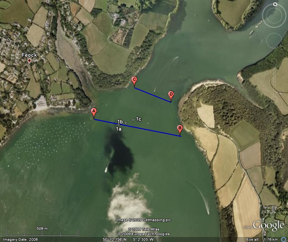
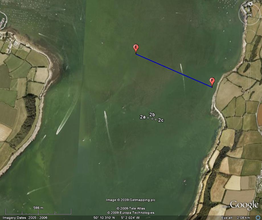
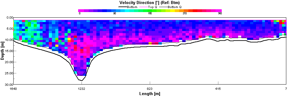
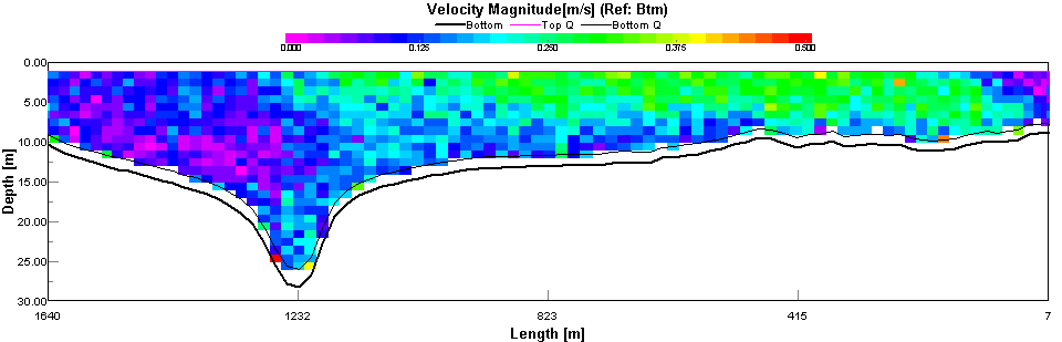
ADCP Analysis

Transect A-B (figure 13) shows a NE flow of 0.5m/s to the East of the main channel (15m deep); and a small region of backscatter in the surface waters in the centre of the river; most likely zooplankton. This northerly flow direction was expected for the flooding tide at this time.

Transect C-D (figure13) shows the same flow speed and direction as it is just north of transect A-B across the shortest part of the river. The backscatter shows two areas at the surface of plankton; one central and one area towards the Eastern shore.

Transect E-F (figure14,16 and 17) shows a deeper channel of 30m, with a NE 0.3m/s flow at the bottom of it, which slows in the surface waters. On the Eastern slope of the channel an eddy can be seen with a 0.1m/s SSE flow. The vorticity here is 1 rotation in 6.3 minutes. A large region of backscatter from plankton can be seen over the top of the eddy, this could be because of the mixing generated by the eddy, re-suspending nutrients needed for phytoplankton growth and therefore predation by zooplankton also colonising this area showing as backscatter.

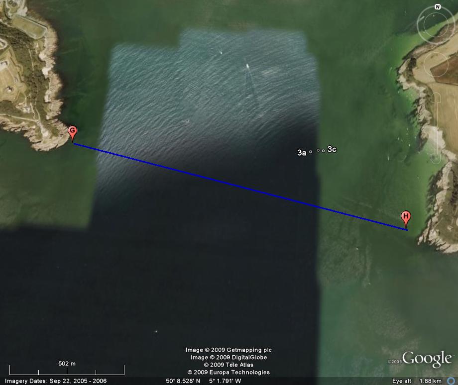
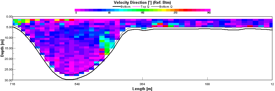
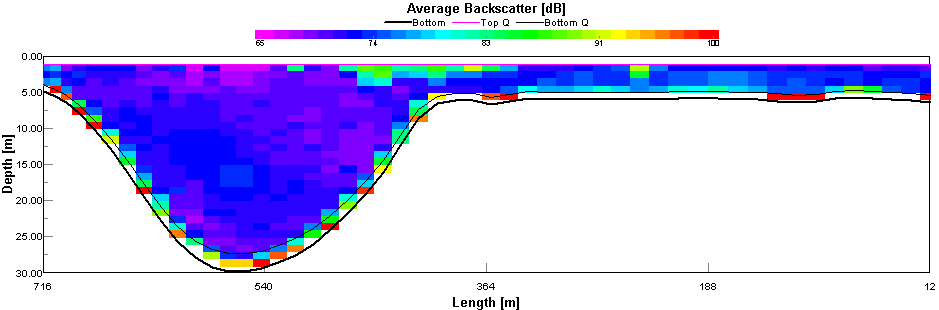
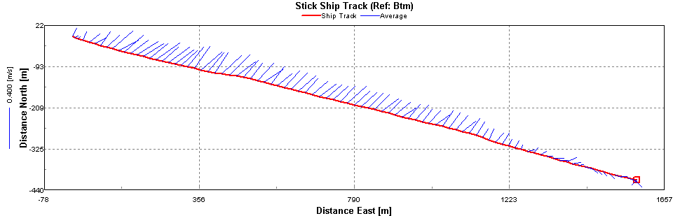
           Figure 16. Velocity direction profile of Transect E-F                                                             Figure 17. Backscatter profile of Transect E-F

Transect G-H (figure 15,18 -20) was a long transect across the whole estuary mouth. The transect profile shows an average depth of around 12m with a single western 30m deep channel. The area to the west of the channel shows the highest flow of ENE 0.4m/s in the surface waters and N 0.2m/s in the deeper waters and channel. Between the Eastern side of the channel and the shore (Shag Rock) the water flow is very mixed; the average water flow is SSE 0.15m/s. Again over this mixing and turbulent region a high backscatter, possibly zooplankton can be seen.

                  Figure 18. Velocity direction profile of Transect G-H                                                       Figure 19. Velocity magnitude profile of Transect G-H

Figure 20. Track plot with stick plots of Transect G-H

Analysis of T/S contour estuary cross sections

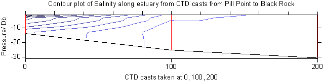
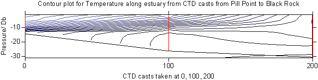
Figure 21.

Figure 22.

CTD casts are marked in red on figures 21-22 with higher salinities and temperatures in lighter shades. The salinity contours range from 29 to 35.5 and the temperature contours range from 13.8 to 18 °C. On both plots the left represents the head of the estuary at Pill Point and the right represents the mouth at Black Rock.

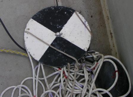
Analysis of the contour plot of salinity clearly demonstrates the Fal estuary is partially mixed. The tidal range taken at St.Mawes is moderate and the tidal currents move the whole water mass up and down the estuary. The tidal range for the 6th July was 3.3m in the middle of the neap/spring cycle occurring on the 2nd and 9th respectively. The riverine end at Pill Point shows some stratification with a salinity range of 4.88 from surface to bottom and the 2nd cast at Saint Just Pool shows a range of just 0.5 salinity. The final CTD cast at the mouth of the estuary shows full homogeneity having a salinity range of 0.05.

The temperature profile shows the riverine end to be warmer and much more strongly stratified with a higher range of temperatures of 2.9 °C. The seaward side is still slightly stratified with surface values of 14.4 and bottom values of 13.8 °C but looking at these values in conjunction with the salinity range, it is clear the water at this point is well mixed with with what could be developing into an oceanic thermocline.

Secchi disk data

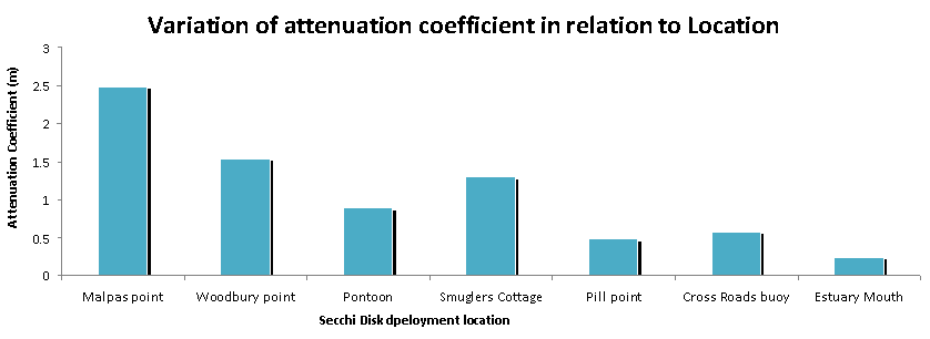
The data from the secchi disk shown in the bar chart above shows an almost consistent decrease in the attenuation coefficient as the water becomes clearer, and has less suspended sediment towards the estuary mouth as there is greater light attenuation. The anomaly at the Smuggler's Cottage location shows a higher attenuation coefficient possibly due to the input of additional sediment from Ruan Creek just before this station. Constant rain squalls all day and heavy rainfall from the previous day could result in greater land erosion and therefore greater eventual sediment transport in the river section. The last three points were all taken in the open estuary section where flow speed was less so particles will settle out resulting in clearer water and will give the result shown of greater light penetration into the water.

CTD Data

Phytoplankton analysis

Table (1) shows the abundance of phytoplankton at three different sites along the estuary. The number of diatoms in the mid-estuary is five times more abundant than the mouth of the estuary. Similarly, dinoflagellates are more abundant in the upper estuary.

What is limiting primary production in The Fal?

Primary Production was high at the river end of the estuary due to high diatom abundance. The diatoms are limited by the amount of silicon in the water. River water contains more dissolved silicon than seawater as the silicon is present in river water due to the weathering of rocks. By the time the river water reaches the sea most of the silicon has been biologically removed to form the silicate frustule of the diatom so less diatoms are present. Dinoflagellates require macronutrients such as nitrates and phosphates for important metabolic growth and other biological mechanisms. These nutrients are present in river water at higher concentrations than sea water for several reasons. Nutrients are being continually added into the river water due to anthropogenic factors such as agricultural runoff, sewage and pollution. Nutrients are also being up-taken by phytoplankton in the river water. By the time the river water reaches the mouth of the estuary there are less nutrients present and the primary production is limited.

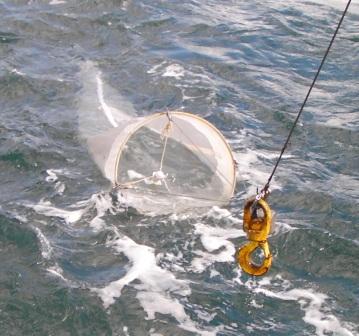
Zooplankton

A zooplankton net was trawled at 2 sites. The families found in these were then counted and compared (figure 18). Overall there seems to be little difference between sites in abundance of families apart from Cladocera and Hydromedusae. No Cladocera was found at site 1 in comparison to 7 at site 2, and the Hydromedusae count was an order of magnitude larger at site 2. This could be due to the jellyfish larvae bring carried around by tidal currents, this could be the reason for the large abundance in the second trawl.

The zooplankton samples collected on MV Xplorer were stored in formalin and analysed in the lab. Samples were placed on a Sedwick rafter slide under the microscope and different families were identified and counted. Phytoplankton samples, were stored in Lugol's iodine. Two ml were taken and placed on a frustle cell, which was then analysed under the microscope in order to quantify cell abundance.

Figure 18

Click to ENLARGE

Estuary Stations nutrient data

For details on all the lab methods used please CLICK HERE

Estuary Mixing

 

Phosphate This represents the mixing diagram for phosphate from the source of the river in Truro, where salinity reaches zero, to the mouth of the estuary. The TDL (Theoretical Dilution Line) was plotted using these riverine and seaward end members. An anomaly can be noticed at the second point which is higher in phosphate than expected. However, looking at the following points a trend can be observed; from the second point onwards the decline in phosphate concentrations is nearly constant to the mouth of the estuary. This anomaly is likely to be due to an extra phosphate input in the river from sewage companies around the area, (such as that found where Calenick Creek joins Truro River) and possibly agricultural runoff. In fact, the input is clearly downstream from the first point where samples were taken at salinity 0, therefore this nutrient behaves non-conservatively due to addition by these sources.	Click to ENLARGE
Nitrate   This represents the mixing diagram for nitrate, from Truro downstream to the mouth of the estuary. By comparing results to the TDL  non-conservative behaviour can be seen where nitrate is removed in higher salinities and therefore towards the open sea. This may be due to biological uptake in the upper estuary where the area is more sheltered and there is less mixing, allowing for a larger biomass population and therefore a higher utilization of nutrients. However, if there were any procedural errors, it is possible that the first point may have been of a lower value, in which case the TDL would shift lower and the points would be even closer to this. In fact, the points would be within the error distance, and this would therefore represent more conservative behaviour .	Click to ENLARGE
Silicon   As the RIB could only reach salinities as low as 25.9 there is a gap on the estuarine mixing diagram where no data was taken (salinity 4.5-25.9); this makes it hard to interpret the behaviour of silicon throughout the whole estuary. It is possible to say however, that the majority of the samples that were collected (salinity 25.9- 35.215) generally show conservative behaviour, possibly with slight removal as they lie just below the Theoretical Dilution Line (TDL). The outliers highlighted are random and are possibly due to contamination or a problem with the collection of the sample.	Click to ENLARGE

Conclusion:

The survey performed on the Fal estuary, yielded numerous trends within the water column, regarding to nutrients, biological and physical parameters. Using this data it can be concluded that there are various different mixing intensities and strategies both horizontally and vertically within the estuary influenced by oceanographic processes and estuarine inputs. This has consequent influences on the light penetration through the water which combined effects the plankton distribution and abundance. 

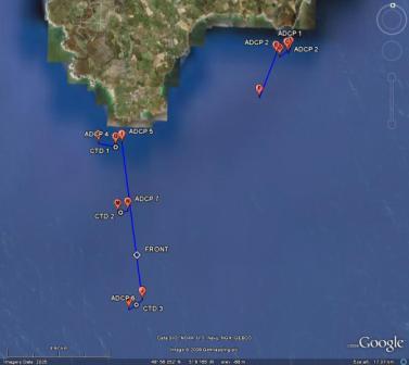
A survey of the offshore region outside the Fal estuary was carried out leaving the Prince of Wales pier on board RV Callista at 07:45GMT. The original plan was to conduct an ADCP profile from Black Head offshore at a perpendicular angle to the headland with a CTD cast at either end. Another ADCP profile would be conducted from Lizard Point offshore with a CTD cast at either end to look at the flow around the headland. The first CTD cast at Black Head took slightly longer than anticipated and a tide line was noticed where water was predicted by the ship's computer to be converging from around Land's End towards Lizard Point and heading South and water coming from the English Channel was meeting it before turning South and heading west. It was decided to take the ADCP across the tide line and two different water types were clearly seen to be going in different directions. This track meant we were no longer able to do our second CTD cast and still make it to Lizard Point, this cast was abandoned. A shallow CTD cast was taken at Lizard Point with the aim of heading offshore to find the thermocline, zooplankton backscatter and evidence of a front on the ADCP. By using a T/S probe we could monitor the increase in SST as an indicator of where the front was positioned. This was found with success and a CTD cast was taken in the channel to depth 75m at position 49°52.868N 005°11.331W and then in the middle at chart position 49°59.157N 005°12.169W to compare nutrient and species distribution across the front. RV Callista returned to berth at 14:00GMT.

Date: 09/07/09

PSO: Aaron Cooper

Boat: RV Callista

Area: Lizard Point

Time: 7:30 - 14:00  GMT

Analysis of contour plot

The temperature contour plot, figure 20, clearly shows coastal mixed waters and offshore thermal stratification. Due to the roughness of the waters inshore as shown on the nautical chart for the region, high mixing is expected with no or minimal vertical stratification. Starting at Lizard point, chart position:49°56.804N 005°12.893W, a CTD cast was taken. The next cast was taken at the most southerly point using the ADCP to determine the position of the front. This position, 5.9km south, showed significant stratification, clearly indicating the front. A CTD cast was taken at this point and it perfectly displayed a developed thermocline as seen on the right hand side of the contour plot. The last cast was taken on the way back to shore 4.3km from our original start point. This midpoint showed the same thermal signatures but at a smaller magnitude.

                                                                     Figure 20

ACDP

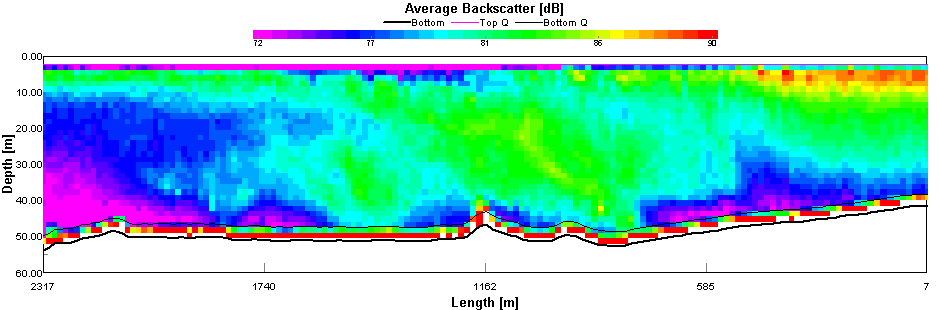
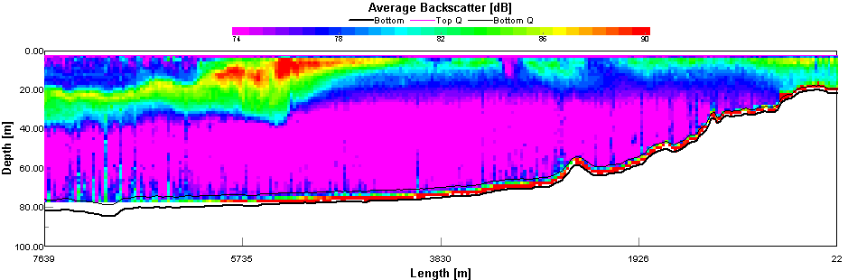
                                                                                       Figure 21. Backscatter for tide line

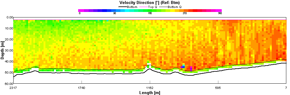
                                                                                     Figure 22. Velocity direction for tide line

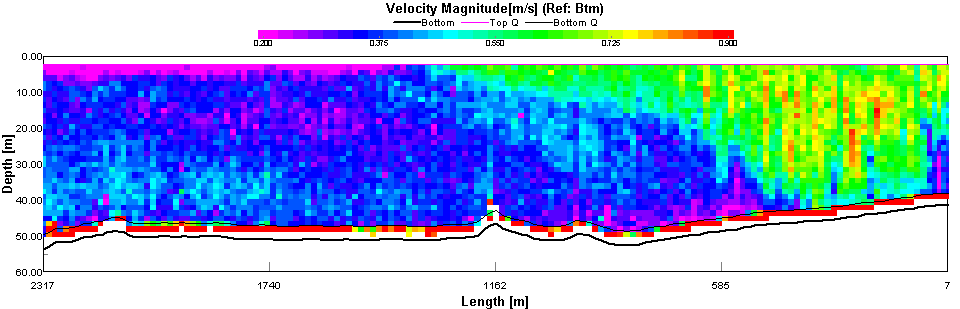
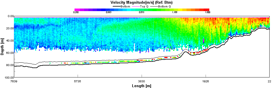
                                                                                     Figure 23. Velocity magnitude for tide line

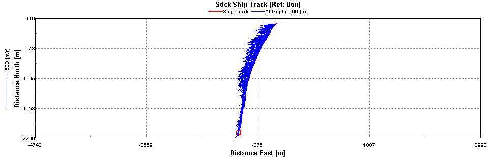
                                                                       Figure 24. Ship track showing stick plot at 4.6m

The first ADCP transect was done over a temporal tide line caused by slack water offshore from Black Head turning east before the shallower inshore waters. This appears as a distinct line with suspended sediments and material in the water caused by shear flow, and is a temporary feature. This is shown by the strong 0.9m/s flow at 265º as expected from 4 hours after height tide. The deeper offshore water is still travelling slowly 0.35m/s at 210º which is the flow from the tidal diamond still from the 3hours after high tide, showing the deeper waters taking longer to turn.

The backscatter shows a high reading throughout the water column as we pass through the tide line, 1km into the transect. This could be zooplankton as the shear flow would create mixing that would stir up nutrients beneficial for phytoplankton growth. But because this phenomenon is so ephemeral this is unlikely and it is more likely to be sediments and other substrates being caught in between the two flows; this causes higher turbidity and backscatter.

                                                                                          Figure 25. Velocity magnitude of front

An ADCP transect, figure 25, was conducted from Lizard Point going southerly to find the boundary between the mixed inshore waters and the stratified offshore waters. An increase in backscatter data in the surface that deepens, and an increase in sea surface temperature are characteristic of a front between mixed and stratified waters.

The inshore waters show high flows at 1.4m/s due to the westerly going tide racing around Lizard Point and slower flow, 0.7m/s, 5km offshore shown by the length scale.

                                                                                           Figure 26. Backscatter showing front

High levels of backscatter at the surface can be seen 5.3km offshore, this is the start of the transition between mixed and stratified water. This area has high surface planktonic activity due to high nutrient levels from upwelling inshore of the front and the high light intensity.

As the transect travels further offshore the maximum backscatter deepens following the thermocline. At this point the plankton causing the backscatter are deeper due to the high nutrient concentrations at 20-40 depth that is still within the euphotic zone. These stratified waters showed warmer surface temperatures due to the reduced mixing, which could be seen and was used as an indicator of the front using a T/S Probe while steaming.

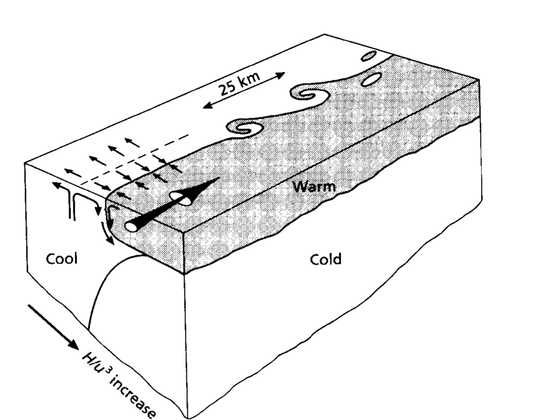
Figure 27. Schematic of a typical frontal system

The Simpson-Hunter Model (H/U^3 factor) for mixed or stratified waters is an arbitrary value that increases with stratification. It shows a sharp increase between the shore and the frontal zone showing a change to more stratified water and then a constant value of 2.35 for the stratified deeper waters. This supports the evidence from the backscatter, T/S Probe and CTD casts.

Richardson Number

                                         Figure 28. Ri for CTD 1

If Ri values are below 0.25, the probability of mixing occurring is high, and if above 1.00 mixing is unlikely (stratified). On the first CTD cast the density shows a shallow thermocline in the surface 5m which produces the high Ri number at 4.6 and 9.1m. The well mixed inshore waters then show most of the values below 0.25 as the waters are well mixed from strong currents in shallow water. The water flow decreases with depth due to bottom friction with the sea bed.

                                    Figure 29. Ri for CTD 2

The second CTD cast in the frontal zone, shows much more variance between stratified and mixed. This is typical of a frontal region and the stratified Ri values correlate with the step changes in density, e.g. at 6.1m. The low flow velocity in the surface could be due to surface friction as the water flow was going east to west and the wind direction was north-westerly. The drop off with depth is most likely due to bottom friction.

                                         Figure 30. Ri for CTD 3

The third cast in the stratified offshore waters show a clear step from the surface thermocline. Either side of this, values are lower than 0.25 showing mixed homogeneous waters. At the transition points the Ri spikes indicate the stratification in this region, e.g. 12.1m Ri=32.21. This also coincides with a drop in flow velocity around the density increase.

At station 1 strong mixing is demonstrated by the uniform nature of salinity and temperature. Below 5m temperature range is between 13.2 and 13.5°C down to 25m.The salinity is fairly stable though being erratic at the surface, possibly due to evaporation or wave action. At station 2 salinity is still constant with depth. Temperature decreases with the initial development of a stratified water column. It gently decreases from 14.7°C at the surface down to 12.3°C at 50m, after which it becomes more stable. At station 3 the water column is fully stratified with rapid temperature taking place between the depths of 10 and 20m. The surface temperature is 15.5°C whilst below the thermocline it is 11.1°C. Salinity is also as stable as in the previous two stations.

Phytoplankton

Table 2 shows the phytoplankton counts at three different offshore stations as seen in figure19. At the station closest to the shore a very high diatom abundance was observed. This high abundance may be due to lots of mixing which may have caused a continuous bloom. This could be an anomalous result as not many nutrients were found in this site. These high figures may be attributed to human error (for example during the phytoplankton counts), as this site has diatom abundance higher than the other sites which were located on the front.

At site 2 the presence of a thermocline shows that the water column is starting to be stratified. Nutrient availability is higher which could explain the large abundance of diatoms and dinoflagellates.

At the tidal mixing front (site 3) two samples were taken at two different depths. The water is highly stratified and there is a distinct thermocline. Due to nutrient addition on the upwelling side of the front these stable conditions are ideal for phytoplankton growth. At 15m depth where the nutrient availability was higher, for example silicon, diatoms were very abundant. Also, the sharp thermocline allowed for a large bloom area. At 5m depth, diatoms are less abundant due to a sudden decline in silicon as well as phosphate.

Zooplankton

The most dominant zooplankton groups present were gastropod larvae and hydromedusae. Gastropod larvae were most abundant at the station closest to the shore suggesting they were the larvae of intertidal species. Hydromedusae were present in large numbers at all three stations. Station 3, located past the tidal mixing front had a lower abundance at the depth we sampled at. As gelatinous plankton are not motile they may have been exported by a downwelling current. Other plankton groups were present at similar levels at all 3 stations; echinoderm larvae, chaetognatha, polychaete larvae and copepoda. Cladocera and siphonophora were found at site 1 only.

For details on all the lab methods used please CLICK HERE

Vertical profiles of Temperature, Oxygen, Phosphate and Nitrate  and Chlorophyll

Conclusion

The offshore survey conducted successfully showing the profile across a tidal front from Lizard Point south into the English Channel. The CTD data for the 3 casts correlate the chlorophyll maxima with the zooplankton backscatter. The ADCP data for backscatter highlighted the presence of zooplankton at the exact location where flow velocity decreased, allowing thermal stratification to take place. The Richardson numbers calculated concur with the data. The nutrient data, although sparse concurred with these findings also with nutrient levels at almost zero at chlorophyll maxima.

The survey of the Fal estuary and offshore region led to many typical characteristics of a partially mixed estuary being highlighted. The RIB data and pontoon time series data show clearly that the whole water body moves up and down the estuary. The calculations of residence and flushing times of 54.8 days and 18.66 days respectively, show that pollution and contaminants in the estuary remain there for a relatively long time and could be having an affect on biota as seen in the past. The geophysical survey of the Helford estuary conclusively proved that anthropological factors are affecting the seabed morphology and the life that can live in these conditions. The offshore survey data ties in with the estuary survey in that the structure of the water column is mixed inshore and stratified offshore allowing stable conditions for phytoplankton growth and zooplankton clearly following them in the water column.

References

www.cycleaucornwall.org.uk/catprofiles/Fal_Helford/physical/hydrology.htm accessed 10/07/2009

Parsons T. R. Maita Y. and Lalli C. (1984) “ A manual of chemical and biological methods for seawater analysis” 173 p. Pergamon.

Johnson K. and Petty R.L.(1983)  “Determination of nitrate and nitrite in seawater by flow injection analysis”.  Limnology and Oceanography 28 1260-1266.

Grasshoff, K., K. Kremling, and M. Ehrhardt. (1999). Methods of seawater analysis. 3rd ed. Wiley-VCH.