![]() Falmouth
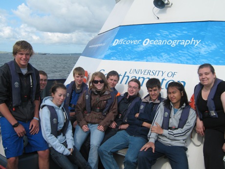
Field Course 2009 Group5
Falmouth
Field Course 2009 Group5
|
|
|
Jon Evans |
![]()
![]()
![]()
![]()
![]()
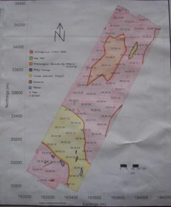
The Fal estuary (Figure 1) is located in Cornwall on the South-West coast of the UK. It is a drowned river valley or ria formed when sea levels rose at the end of the last ice age approximately 10,000 years ago. The estuary extends from its entrance between Pendennis Point and St Anthony Head to its tidal limit at Tresillian 18km inland. It is the third deepest natural harbour in the world and therefore important for maritime trade, tourism and conservation of landscapes, habitats and species.
The estuary can be sub-divided into two parts, the outer tidal basin and inner tidal tributaries. The outer tidal basin known as Carrick Roads contains about 80% of the water within the estuary. It is characterised by a deep channel which meanders through the estuary with depths of up to 34m. The channel shallows to 12m as it reaches Turnware point before continuing through King Harry Reach as the river Fal with a depth around 5m. The inner tidal tributaries consist of 6 main tributaries and 28 minor creeks and rivers which all eventually flow into Carrick Roads. The rising sea levels have also lead to the formation of extensive wetlands in parts of the upper estuary. The estuary is macrotidal with a maximum spring tide of 5.3m at Falmouth becoming mesotidal at Truro with a spring tide of 3.5m (Pirrie et al.). The maximum tidal current is usually below 2 knots.
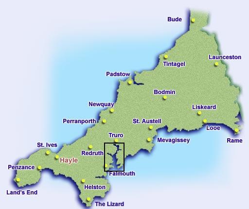 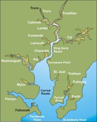 Figure 1: Maps of Cornwall to show the location of Falmouth and the Fal estuary. |
Together the Fal and Helford estuaries have been designated as a Special Area of Conservation (SAC) due to their support of rare, endangered or vulnerable habitats and/or species, as listed in the Annexes I and II of the Habitats directive (Fal and Helford Management Forum, 2006). These areas are labelled as ‘interest features’ and in terms of the Fal and Helford SAC include inter alia. mudflats, maerl beds (Phymatolithon calcareum), Eelgrass (Zostera marina), shore dock (Rumex rupestris), subtidal sandbanks and saltmarshes. In total the SAC covers an area of 6387.8 ha (JNCC) However the species and habitats protected by the SAC designation are under threat from properties of the Fal estuary and catchment. The catchment area is predominantly rural and supports intensive mixed arable and dairy farming leading to eutrophication in some areas of the estuary. Although the majority of the nutrient inputs into the SAC may be due to diffuse sources from the agricultural runoff, sewage treatment works such as the Truro Newham Sewage Treatment Works are significant in the more enclosed areas of the estuary where the chronic contamination and high nutrient loading has led to toxic algal blooms. An example is the 1995-1996 bloom of the dinoflagellate Alexandrium tamarense. |
Mining for primarily Sn, Cu, Pb and Fe has been a major activity in the area since the Bronze Age and peaked in the 19th century. In particular, ore processing in the Carnon Valley remobilised millions of tons of tailings which have been deposited in the Restronguet Creek making it the most metal polluted estuary in the UK (Bryan and Langston, 1992). This has lead to the Restronguet Creek dominating metal inputs, particularly As, Cu, Zn, Cd and Fe, into the Fal estuary for centuries.
There is little large industry left to affect the Fal sediments and water quality. However Falmouth docks and a number of marinas are continual sources of disturbances through processes such as dredging, oil spills and release of antifouling and sewage. Indeed, the extensive use of tributyl tin (TBT) in the past has lead to the whole system being affected by organotin contamination. Although the principle source is the Falmouth Dockyard, re-release from sediments now also contribute significantly to the overall load (Langston et al. 2003). Although banned on boats since 1987, the concentration still exceeds the EQS of 2ng/L. The main effect of TBT contamination is imposex in Dogwhelks.
The overall aim of the field course is to investigate the chemical, biological and physical properties within the estuary and off-shore to enable understanding and quantification of the interactions between them, both within the water column and with the processes within the surrounding catchment area. To this end, a chemical and biological survey will be carried out both in the estuary and off-shore as well as a geophysical survey with the aim of creating a benthic habitat map within the estuary itself.
|
Boat Information |
|
|
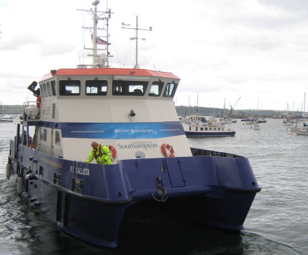
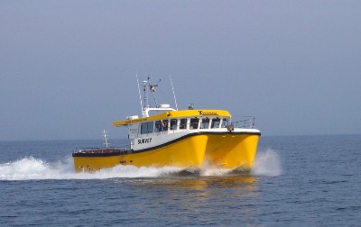
RV Callista The RV vessel Callista is a 20 metre catamaran used for offshore research to measure a range of oceanographic processes. It is equipped with both wet and dry laboratory facilities and a large stern deck. It is capable of deploying large equipment using an ‘A’ frame. Callista also has two davits either side which can each take weight of up to 100 kilograms to lower midsized equipment. Specifications Equipment
|
|||||||||||||||||||||||||
|
|
SV Xplorer This vessel can survey both inshore and offshore and is equipped to deploy midsized equipment from the open stern deck for bathymetric surveying such as what was carried out in the geophysical survey. Specifications Equipment
|
|||||||||||||||||||||||||
|
|
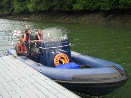
Ocean Adventure RIB The Ocean Adventure RIB is a ridged inflatable vessel (RIB) which is quick and easy to manoeuvre therefore allowing an increased sampling time at distant stations. It is also able to access shallow areas of the Upper Fal due to its shallow draft and lift-able engine, but can only deploy small equipment. Specification
|
|
CTD
Plankton net
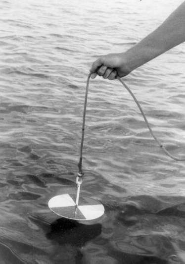
Secchi disc
|
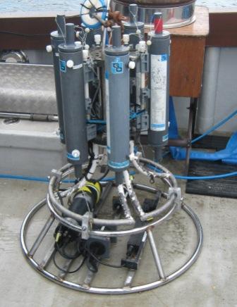
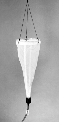
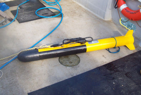
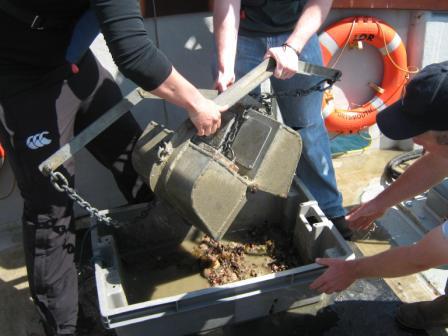
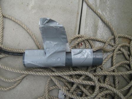
Sidescan sonar This allows the seabed topography to be mapped including contrasting sediments. A transducer in the tow fish emits a wedge-shaped sound pulse which is reflected off the seafloor. The returning intensity is measured and displayed for the operator to analyse. A strong reflection indicates a slope facing the towfish whilst low backscatter values indicate softer sediments. Areas of no return, or 'shadows' are slopes facing away from the sonar which are steeper than the angle of the sonar beam. A 2-dimensional picture of the seabed is produced in black and white with saturation intensity giving an indication of roughness, slope and shadowing showing bedforms. Van Veen Grab This is used to obtain a sediment sample of 0.25m3 using a claw mechanism which is released when the weight is taken of the chain as it hits the seafloor. A sharp edge allows the claws to easily cut through soft sediment but is not as effective on coarse sediment. The sample collected is normal greatly disturbed and some of the sample can be lost on retrieval. Mainly used to study the benthic community at grab sites. A CCD video camera This was lowered over the deck at each grab site to assess whether the sidescan was accurate and if it was an area that needed to be sampled. It provided an undisturbed overview of the benthic habitat on the seabed, as well as preventing disturbance of protected seagrass beds Zostera sp. Applied Microsystems Smart CTD This is used to measure salinity, temperature and depth. Six Niskin bottles in a rosette system are attached, along with a transmissometer to measure suspended sediment concentration, a fluorometer as a proxy for chlorophyll concentration, a sensor for light (Li Cor sensor) and a sensor for dissolved oxygen (this sensor was un-calibrated and therefore its data were unreliable). The CTD is linked to a computer via Smart Capture, which captures the data as it is measured so graphs can be plotted onboard. The Niskin bottles can be triggered individually which enables samples to be collected at depths determined from the Smart Capture data. ADCP (Acoustic Doppler Current Profiler) The ADCP was used to measure the current flow velocites (speed and direction) across the estuary, and can also show particulate matter in the water column by backscatter. It works by sending out sound pulse that get doppler shifted by moving water parcels to higher or lower frequencies depending on whether the water parcel is moving towards or away from the ADCP respectively. Three sound beams in different planes are used to build up a full profile of current magnitude and direction. Secchi Disk A black and white disk which is used to measure the attenuation of light in the water column. When the secchi disk can no longer be seen the depth is measured from graduations on the lowering rope. This depth 'the secchi depth' is multiplied by three to give the depth of the euphotic zone. T/S Probe This contains a thermistor and set of conductive plates which measure temperature and salinity respectively. It is used to measure the temperature and salinity every 5 minutes to produce a temperature and salinity profile for the estuary. Plankton Net A 200um mesh size plankton net with a 500ml bottle was used to collect samples of zooplankton to be quantified in the lab. A closing plankton net is used to collect samples from specified depth ranges. |
Sidescan sonar towfish
Van Veen grab
CCD video camera |
![]()
![]()
![]()
![]()
![]()
![]()
|
Aim |
To map the benthic marine habitat and seabed lithology along the east side of the Fal estuary to explain how the physical environment effects biological distributions within the Fal estuary.
|
Introduction |
On 01/07/2009, a geophysical survey was conducted in the Carrick Roads region of the Fal estuary, near Saint Mawes Harbour. The survey area, Saint Mawes Bank, was determined suitable by looking at chart depths, tide heights, boat draft and tow fish depth to ensure there was always enough water under the hull. The rising tide was utilized throughout the morning to allow the shallower water to be surveyed. Saint Mawes Bank is the location of the largest maerl (Phymatolithon calcareum) beds of their type in England and Wales and they provide shelter to a wide variety of different, rare flora and fauna
|
Weather
|
Tides
|
|
Method |
|
A benthic sea survey was completed on the east side of the Fal estuary on the 1st July 2009 between 0800-1300 GMT using SV Xplorer as the survey platform. Four lines, each about 1.5km in length and approximately parallel to each other were surveyed and mapped using the sidescan sonar at a frequency of 100 kHz and a speed of 4 knots. Time, position, depth and other observations, including wakes of boats that might affect the sidescan sonar readings were recorded. Several possible grab sites were identified from the sidescan sonar trace as it was being produced. The underwater video camera was lowered first to check grab suitability, then the Van Veen grab was lowered to take benthic marine samples. Samples were transferred into a tray, from which the sediment type was identified, as well as marine benthic species using Guide to the Sea & Shore Life of British and North-West Europe. The sample was then wet sieved using a 2.5mm sieve on top of a 1mm sieve to remove the smaller sediments and identify the major substrate/habitat present. On returning to the lab, the continuous sidescan sonar trace was separated into each transect and interpreted. Calculations were done on the features observed to determine their position and characteristics such as height. After identifying the features and their positions, the data was transferred onto a smaller track plot which was produced using Surfer software. |
Figure 2: Track plot produced on Surfer, then annotated by hand. |
|
Results |
Survey Line Locations:
|
Line number |
Position |
Time (GMT) |
Depth (M) |
|||
|
1 (13) |
50˚09.434 |
50˚10.102 |
08:34 |
08:44 |
32.9 |
4.7 |
|
2 (14) |
50˚10.085 |
50˚09.340 |
08:46 |
08:57 |
4.4 |
11.2 |
|
3 (12) |
50˚09.364 |
50˚10.140 |
09:00 |
09:10 |
9.2 |
5.4 |
|
4 (11) |
50˚10.161 |
50˚02.389 |
09:13 |
09:25 |
5.7 |
9.0 |
For analysis, the separated sidescan traces were attached together to form a mosaic. Areas of interest such as tonal changes and bed forms were highlighted and measured. Using the navigation data collected through the sidescan software, a track plot was created onto which data from the sidescan trace was transcribed. The specific areas of interest indentified are described below.
 |
 |
 |
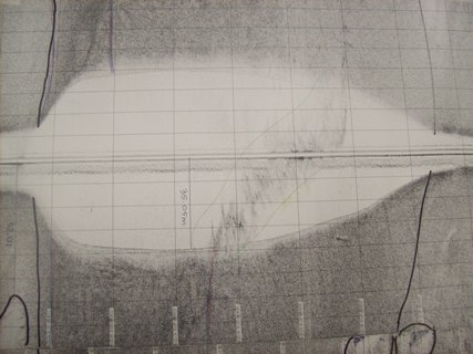
| Figure 3: Sidescan sonar
plot of the deep channel |
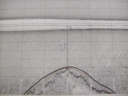
Figure 4: sidescan sonar
plot of the coastline |
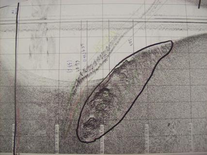
Figure 5: sidescan sonar
plot of the rock outcrops |
Sidescan Sonar Track Plot Analysis
Most of the seabed analysed was homogeneous maerl beds, as predicted, with few defining sediment characteristics.
Carrick Roads Channel
The main feature of the track plot is the Carrick Roads Channel running across the south side of the plot. The channel was naturally formed by the river channel before the estuary became a ria. It has a maximum depth of 35.05m and has very steep walls with depth changing from 6-8m outside the channel to below 30m depth within 50m (figure 3). The channel itself had defining characteristics; the sediment was far coarser, indicated by the darker tone from greater backscatter, due to the stronger current removing much of the finer sediment.
Rocky Outcrops
There are also rocky outcrops within the channel between the time stamps 08:36:04 and 08:56:20. The height of the largest outcrop shown in figure 5 varies between 0.35m and 1.93m, the tallest point being on the left side of figure 3. There are also trenches along the south edge of the channel either side of time stamp 09:01:45. This may be where strong currents moving from the shallow water into the channel have scoured out trenches into the channel.
Coastline
Samples were taken as close to shore as possible to collect as much information on the maerl beds. The sidescan sonar picked up rocky outcrops from the coastline from time stamp 08:51:59 - 08:53:49 and 08:46:19 – 08:48:51, shown in figure 4.
Anthropogenic Features
Anthropogenic features were also noted on the sidescan mosaic. A very straight trough was picked up between time stamps 09:01:24 – 09:24:50 which could be an anchor line or from a trawl being dragged along the bottom. A large area of anthropogenic features were found around time stamps 09:09:24 -09:06:54 including many dredge marks and anchor lines suggesting an anchoring or fishing area.
|
Grabs |
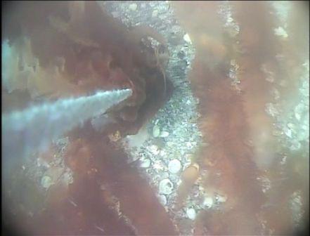
Four locations were chosen to take grab samples. Their locations were determined from slope and tonal changes identified on the sidescan trace representing interesting features. Firstly an underwater video camera was put into the water to check site suitability for grabs, before a Van Veen grab was lowered to collect the sediment in 0.25m3 sized samples.
 |
 |
 |
 |
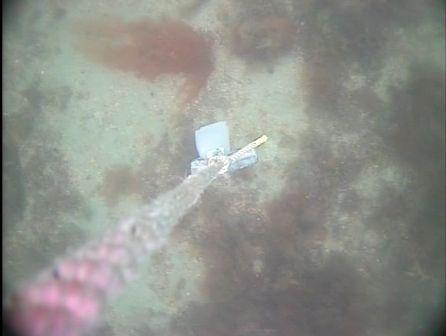 |
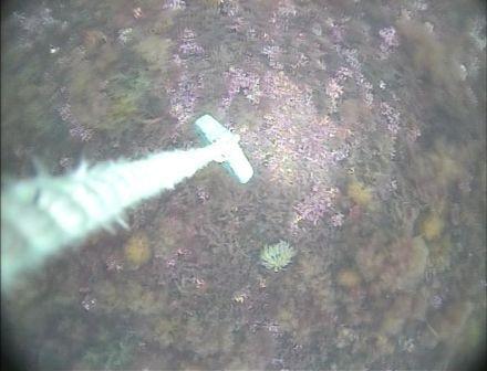
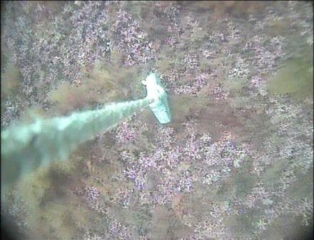
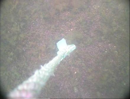
| Figure 6: Site of grab 1 as seen through the video camera. | Figure 7: Site of grab 2 as seen through the video camera. | Figure 8: Site of grab 3 as seen through the video camera. | Figure 8a: Possible grab site, not used as felt to be too similar to other grab sites especially 3. | Figure 9: Site of grab 4 as seen through the video camera. |
The sediment within each grab was analysed with a grain size analyser before removing the larger biological specimens for identification. Each grab was then wet sieved through a 2.5 mm and then a 1mm sieve. Material retained in each sieve was analysed whilst small biological specimens were removed for identification.
Grab 1
|
Camera |
Grab 1 |
|||||||
|
Position |
Depth (m) |
Time (GMT) |
Position |
Depth (m) |
Time (GMT) |
|||
|
In |
Out |
In |
Out |
In |
Out |
|||
|
50˚09.676 |
50˚09.552 |
10.2 |
13.0 |
09:56 |
10:02 |
50˚09.504 |
10.8 |
09:58 |
(Camera and grab position, depth and time of grab 1)
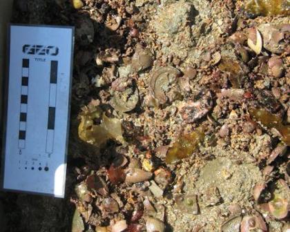
Grab sample 1 (figure 6) was taken south of the main channel and consisted of very fine biogenic sediment between 3-4Φ (0.13-0.06mm) interspersed with larger coarse granules greater than 1mm (figure 10). The lack of a redox potential discontinuity layer (RPD) suggests a strong current oxygenating the sediment or lack of organic matter. A large volume of dead and alive maerl nodules were also present approximately 1cm in diameter.
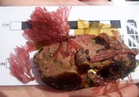
Organisms found included Chitons, many bivalve shells (along with keel worm tubes), the amphipod Scytosiphon lomentaria and long clawed porcelain crabs, Pidonotus claba. Algae species found included Petalonia fascia, Dictyopteris membranous, Palmonia palmate, Rhodymenia pseudopalnata and Ptilota gunneri. There were large amounts of algae as the coarse sediment provided purchase and hold-fasts and the strong current provides the algae with clean water (figure 11) , whilst small invertebrates were able to burrow between the coarse grains. Deposit feeders were limited by lack of organic matter.
 |
 |
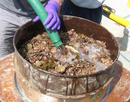 |
| Figure 10: Grab 1 sample | Figure 11: Lomentaria articulata, a red algae | Figure 12: Sieving sample 1 showing both the 2.5mm and the 1mm sieve |
Grab 2
|
Camera |
Grab 2 |
|||||||
|
Position |
Depth (m) |
Time (GMT) |
Position |
Depth (m) |
Time (GMT) |
|||
|
In |
Out |
In |
Out |
In |
Out |
|||
|
50˚09.729 |
50˚09.783 |
7.3 |
7.3 |
10:30 |
10:44 |
50˚09.729 |
7.0 |
10:33 |
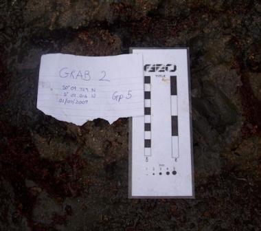
(Camera and grab position, depth and time of grab 2)
Grab sample 2 (figure 7) was taken on the north side of the main channel and showed that sediment in this region of the estuary is mainly silt and clay, <4Φ (<0.06mm) possibly resulting from a drop in current strength. The sediment was interspersed with small maerl nodules (2cm diameter) both dead and alive. The maerl was healthier at this site, which contrasts with the literature that states that fine sediment smothering is a hazard towards maerl populations. The Sediment showed a RPD layer at 1-1.5cm, indicating reducing conditions. The 2.5mm sieve retained living and dead maerl, bivalve shells, some seaweed and very course sediment. The 1mm sieve retained dead maerl nodules, coarse granules >1mm and no significant biology.
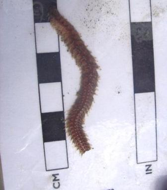
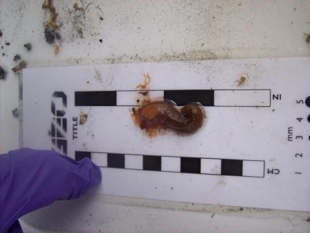
Biology collected included much more infauna than found in grab 1, as the sediment is finer. Suspension feeders were also found in small numbers. Tubes of organisms were composed of small maerl fragments, sediment and molluscs such as Lacuna vincta and Turritella communis. Other organisms found included the polychaete worms Eupolymnia nebulosa (figure 16), Nereis diversicolor (figure 14) and a gastropod, Turban Topshell (figure 15), and Jassa falcata (figure 17).
 |
 |
 |
 |
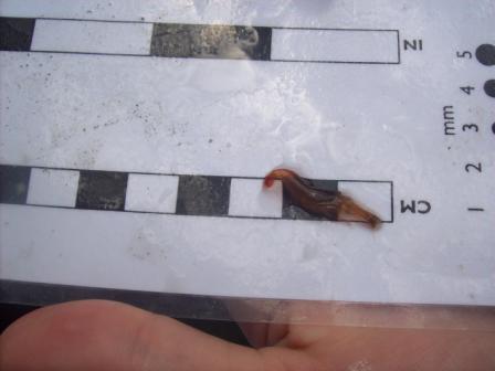 |
| Figure 13: Grab 2 sample | Figure 14: Nereis diveriscolor - this rag worm burrows in muddy sand typically in sheltered inlets and estuaries | Figure 15: Turban topshell, Gibbula magus - found on lower shore and sublittoral to 20m | Figure 16: Eupolymnia nebulosa - this Terebellid Polychaete lives in muddy sands usually in tubes consisting of mineral particles loosely held together by mucus | Figure 17: Jassa falcata, this amphripod is found in both the intertidal and sublittoral zones among algae and hydroids |
Grab 3
|
Camera |
Grab 3 |
|||||||
|
Position |
Depth (m) |
Time (GMT) |
Position |
Depth (m) |
Time (GMT) |
|||
|
In |
Out |
In |
Out |
In |
Out |
|||
|
50˚09.878 |
50˚09.953 |
6.0 |
6.6 |
10:49 |
10:55 |
50˚09.913 |
6.4 |
10:55 |
(Camera and grab position, depth and time of Site 3)
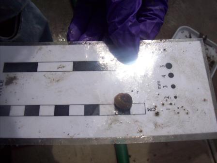
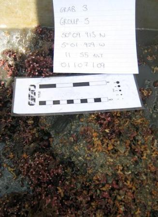
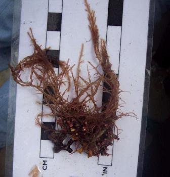
Grab 3 (figure 8) was the shallowest sample taken closest to Saint Mawes Bank and had the finest sediment found, <4Φ (<0.06mm) (figure 18) suggesting a sheltered area and weak currents. Again, conversely, this grab showed the greatest and largest nodules of maerl with an average diameter of 5cm (figure 19). This sediment showed reducing conditions 2cm deep suggesting large amounts of organic matter was present. After sieving with a 2.5mm sieve, all maerl was retained and was mostly alive with some dead. After sieving with a 1mm sieve very little was retained indicating very fine sediment. Due to the high maerl content biomass and biodiversity was greatest in this grab.
Organisms found included Xantho incisus (figure 20), Galathea squamifera (figure 21), Liocarcinus depurator, Jassa falcata and Callianassa suvterrane.
|
|
|
|
|
|
Figure 18: Grab 3 sample. |
Figure 19: Maerl, Phymatolithon calcareun - this is a calcareous algae found in the littoral and sublittoral zones. |
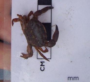
Figure 20: Xantho incisus - this crustacean is found in the lower shore and shallow sub littoral to about 40m. |
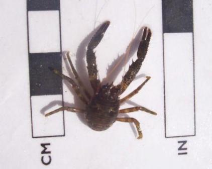
Figure 21: Galathea squamifera - this species is the most commonly found squat lobster. It is found beneath rocks on the lower shore and shallow sublittoral. This crustacean feeds on suspended detritus. |

Grab 4
|
Camera |
Grab 4 |
|||||||
|
Position |
Depth (m) |
Time (GMT) |
Position |
Depth (m) |
Time (GMT) |
|||
|
In |
Out |
In |
Out |
In |
Out |
|||
|
50˚09.687 |
50˚09.683 |
7.1 |
7.5 |
11:25 |
12.29 |
50˚09.683 |
7.5 |
11:29 |
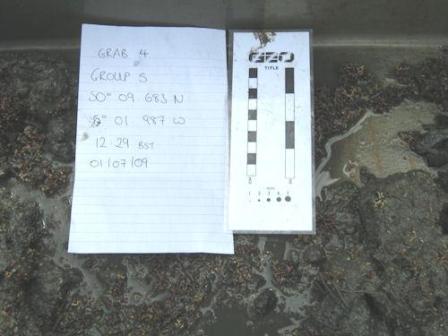
(Camera and grab position, depth and time of grab 4)
Grab sample 4 (figure 9) consisted of very fine sediment 3-4Φ (0.13-0.06mm). On average there was a smaller amount of maerl collected with a diameter around 1cm. There was an RPD layer at 3cm depth. Sieving with 2.5mm sieve retained both living and dead maerl, as well as a small number of bivalve shells and many worm tubes. Sieving with a 1mm sieve retained small granules and maerl nodules, with a larger overall volume than in grab 3. There was significantly less biology in this grab than in grab 3, concurrent with the lower volume of maerl which is known to increase biodiversity. Organisms found included Capitella capitata (figure 23), an indicator species tolerant of polluted benthos. It is an R-selected, opportunistic species allowing it to reproduce rapidly and therefore out-competes other species whilst coping with constant disturbance. Other species found were Nereis diversicolor, Eupolymnia nebulosa and Carcinus meanus. Algal species found included Corallina elongate (figure 23), Scolelepis squamata, and Ulva lactuca.
 |
 |
 |
| Figure 22: Grab 4 sample. | Figure 23: Capitella capitata - this polychaete is an opportunistic species commonly found in areas of high organic pollution. | Figure 24: Corallina elongate - this is a red algae found in the lower intertidal zone. |
|
Summary |
|
Overall the results of the geophysical survey and benthic habitat map concur with previous work done in this area. Analysis of the sidescan mosaic showed the area to be primarily homogenous maerl beds interspersed with inter alia. anthropogenic markings, the deep channel and rocky outcrops. The location of the maerl beds agree with the World Beneath the Waves benthic habitat map seen in Figure 25. Overall the grab samples showed a general increase in maerl density with distance from the channel and finer sediments, closer to Saint Mawes Bank (grab 3). The distribution according to sediment size is opposite to what would be expected from previous studies, so other factors such as pollution may be exerting a greater control on the maerl distribution than sediment size. |
Figure 25: Benthic habitat map of the Fal and Helford estuaries. |
![]()
![]()
![]()
![]()
![]()
![]()
|
Aim |
To explore the physical, chemical and biological interactions of the Fal estuary and to study the effect of differnt biological and physical conditions on planktonic communities. Finally to examine the mixing characteristics of the estuary and develop an understanding of how the freshwater inputs affect the estuary.
|
Introduction |
To fulfill the aim above, the biological, physical and chemical characteristics of the Fal Estuary were sampled both spatially and temporally on the 04/07/2009. During the morning, data were collected in the upper part of the estuary with half the group aboard Ocean Adventure RIB and the others gathering data from a fixed point, the King Harry Pontoon, to build a temporal picture of the chemical, physical and chemical characteristics over the tidal cycle. During the afternoon data were collected on board the S/V Xplorer at the seaward end of the estuary.
Even though the Fal estuary is fed by many creeks, rivers and tributaries it has limited freshwater inputs. This is due to it being a ria, which is rather an extension of the sea than a true estuary. This makes collection of low salinity samples fairly challenging, which is a limitation of the data for this section.
|
Weather
|
Tides
|
|
Methods |
King Harry Pontoon - 50°12.958 N, 05°01.673 W
Data were collected every 30 minutes to create a time series from 09:00 GMT using a YSI probe to measure depth, temperate, salinity, pH and oxygen concentration at 1 metre intervals and at the surface. Water samples were taken every hour using a Niskin bottle at 4 metres and at the surface. From these samples the silicon, phosphate, nitrate and dissolved oxygen concentrations were determined. The samples were filtered before being put in sample bottles, and these filters were submerged in acetone to break the cells down enabling chlorophyll measurements to be taken in the lab.
Ocean Adventure RIB
Data were collected from the RIB at 5 different stations, beginning at the top of the estuary and moving towards the lower estuary, against the tide. At each station the YSI probe was lowered and data collected at half metre intervals. Water samples using a Niskin bottle were taken at the surface to determine concentrations of the above mentioned constituents.
SV Xplorer
Data were collected in the afternoon at 3 different stations. At each station the CTD was lowered and the data were captured during the descent to plot depth profiles. These were then used to find interesting features within the water column to determine at what depths water samples would be collected. Six Niskin bottles were used for the sampling, two from each depth. Every 5 minutes the temperature and salinity were recorded using a T/S probe and the position was also noted. At each station a Secchi disk was used to measure light attenuation and hence the euphotic depth. The phytoplankton trawl net (200um mesh, 500ml bottle) was deployed at two different sites, one at the top of Carrick Roads, and the second at the mouth of the estuary between Pendennis Point and St Antony’s Head. At the same sites the ADCP was used to measure the current flow across the estuary.
|
Analytical Procedures |
|
Nitrate
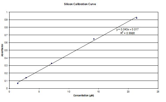
Phosphate and Silicon
Dissolved oxygen
Chlorophyll |
Detection limits for nutrient analysis.
Any concentrations below these values has been set to zero.
|
|
Results |
Physical Structure
|
Figure 26 shows a range of graphs made from the YSI Multiprobe data collected on the Ocean Adveture RIB, and CTD data collected on the SV Xplorer. RIB Station 1 (see Table 1 for locations of RIB stations) was collected at Malpas, with four subsequent stations taken down the river towards the mouth of the estuary. The CTD data was collected at three separate sites, the first at the head of the Carrick Roads, and finishing at the mouth by St Anthony Head. The RIB data generally showed that surface salinity increases down the river towards the estuary mouth, from roughly 17 to 32. This is due to the increase in the seawater component in the estuary. The figure also shows that salinity increases with depth due to the fresher river water flowing over denser salty water. Temperature decreases with depth, with the greatest change recorded at Station 4, which decreases from 19.9ºC to 18.1ºC. Heating of the surface waters by the sun, produces a temperature gradient with depth due to the low heat conductivity of water. There appears to be a weak thermocline at Stations 2 and 5. Conversely, at Station 1 the temperature increases although only by 0.4ºC. However, unlike salinity the surface temperature does not vary down the river, with all stations maintaining a temperature of roughly 19ºC. At Stations 1, 4 & 5 dissolved oxygen decreased with depth, for example Station 4 it decreases from 94.1% to 86.9%. It is thought that this is due to high levels of primary production at the surface with decreased levels at depth due to light attenuation. Station 2 has an increasing oxygen level with depth from 78.2% to 83.6% and Station 3 shows some variation in the top 2m, but the levels then remain constant below this depth at around 83.6%. The figure shows dissolved oxygen to also increase down the river, with Station 1 recording 73.8% and Station 5 97.7% possibly as a result of eutrophication in the upper estuary increase biochemical oxygen demand. The final parameter recorded at each RIB station was pH. All stations display very little change and range from 7.8 to 8.3, therefore suggesting that there is no significant difference in pH with depth. The first CTD Station (Table 2) was at the head of Carrick Roads. Here salinity increased with depth from 28.6 to 33.9. However the next two stations show very little change with depth as can be seen in Figure 27. Temperature decreased with depth at all stations, similar to the RIB Stations. Each station appeared to have two thermoclines, one near the surface (0 – 10 m) and one at depth (10 – 20m) representing a stratified water column. The fluorometer readings (which are a proxy for chlorophyll concentrations) increased with depth to between 4 and 8 metres, before decreasing. This increase is due to increased primary production. The decrease is caused by a decreased irradiance causing a drop in primary production. Transmissometer readings display a slight decrease at the surface corresponding to the increasing fluorometer readings at Station 1, yet in the other stations there seems to be no correlation between turbidity and the fluorometer readings. |
Figure 26: graphs from the RIB data
Table 1: RIB station locations
Figure 27: graphs from the CTD data
Table 2: CTD station locations |
||||||||||||||||||||||||||||||||||||
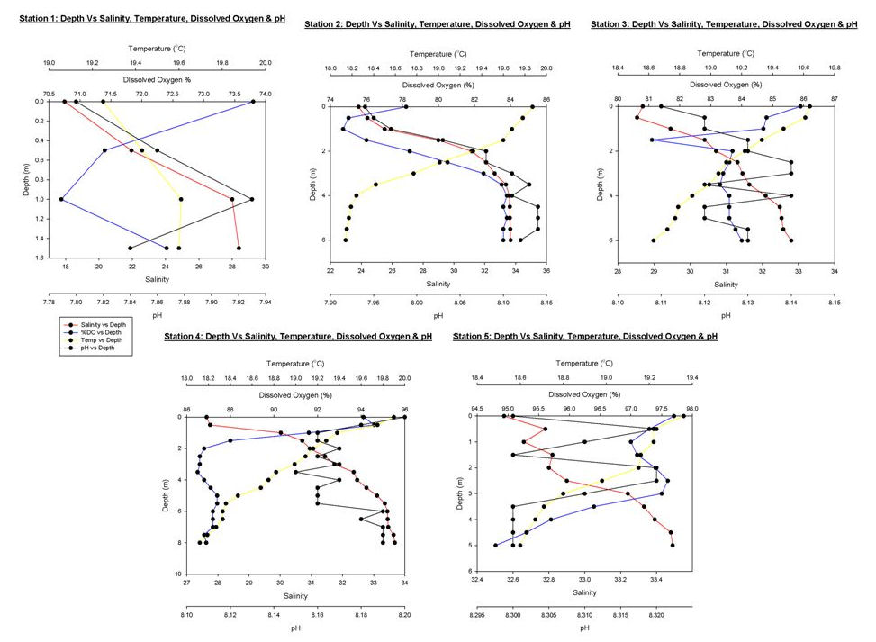
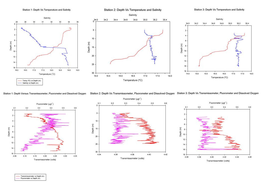
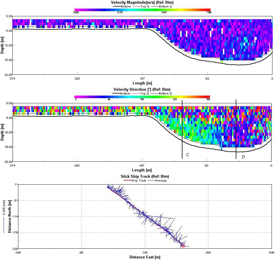
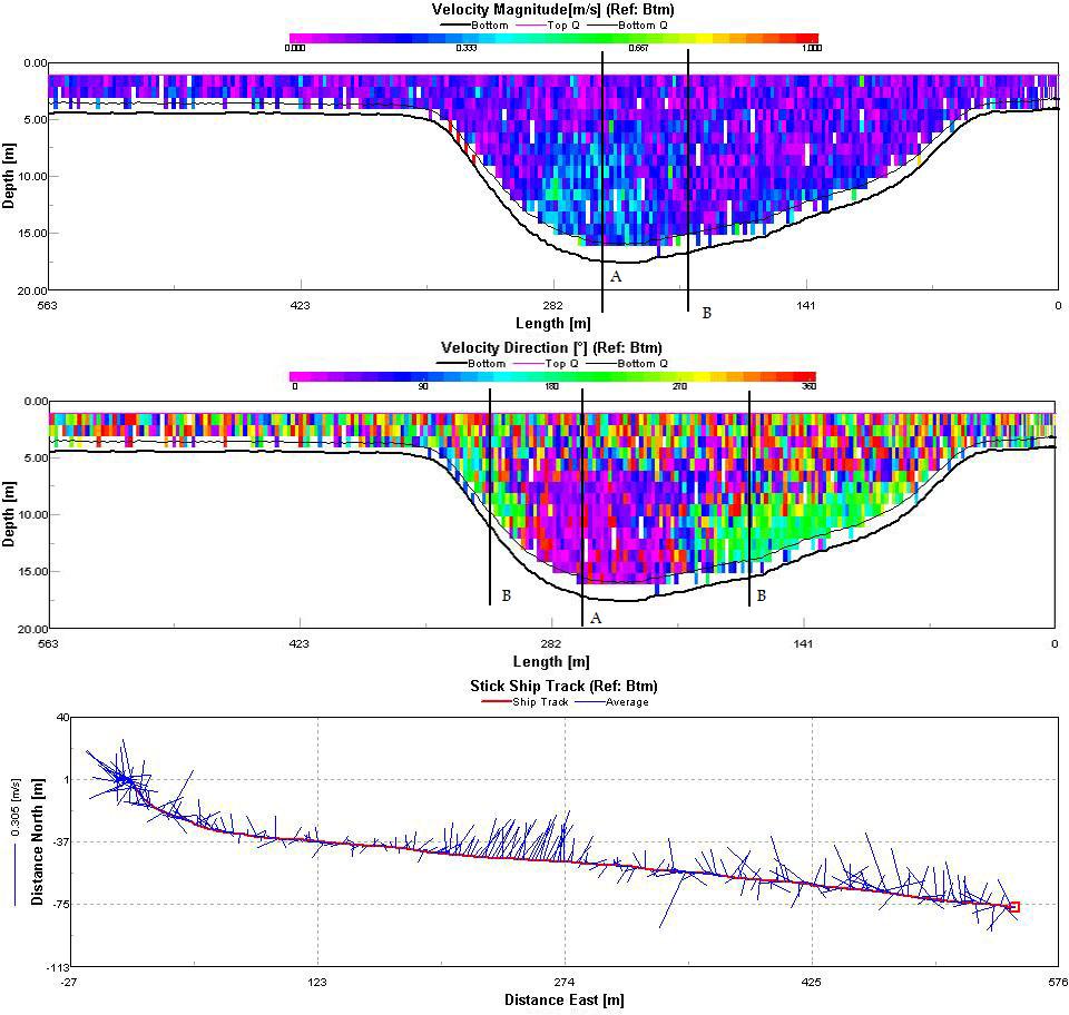 Figure 30: ADCP Track 1
Figure 31: ADCP Track 2
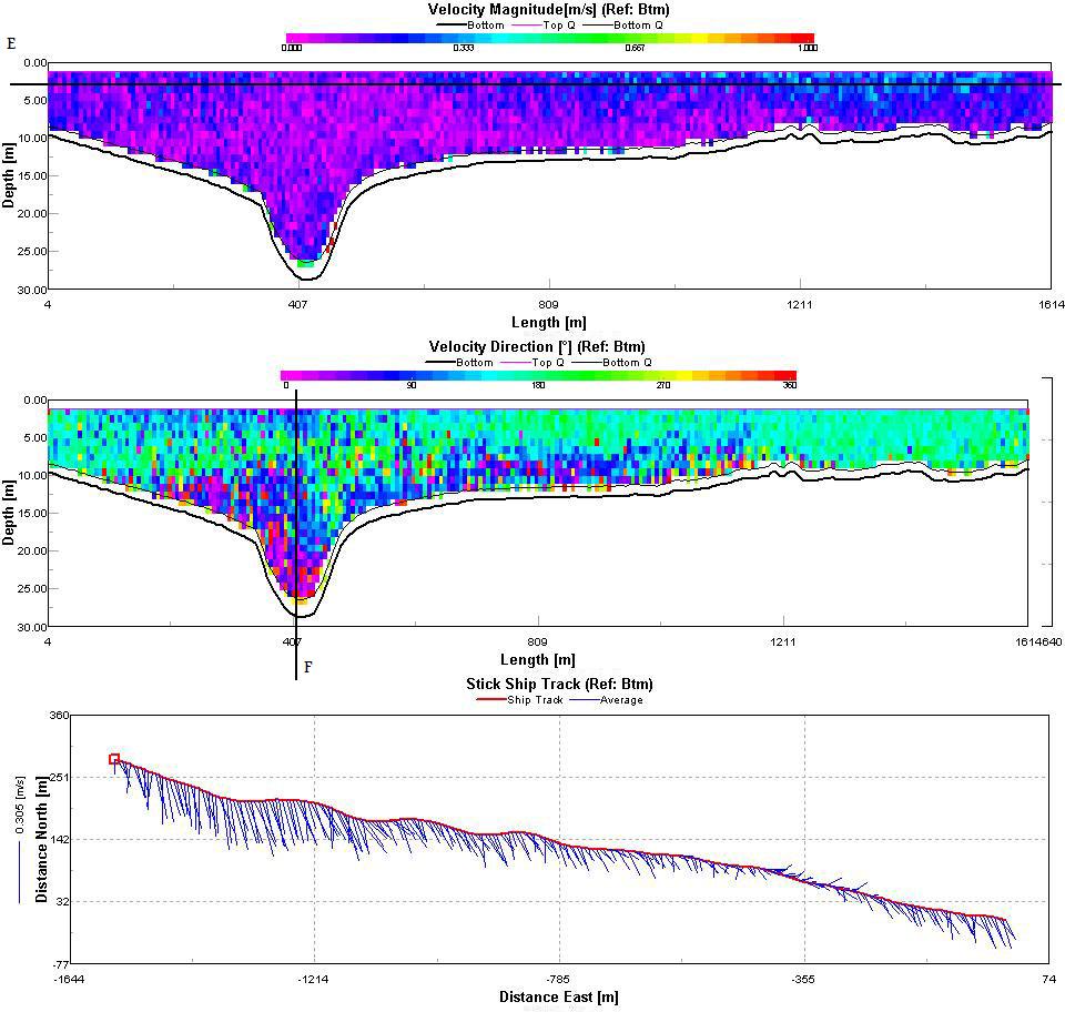
Figure 32: ADCP Track 3 |
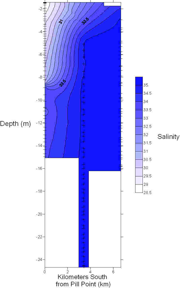
The Fal estuary can be classified as partially/well mixed depending on the spring neap cycle. This conclusion is supported by the position of the temperature and salinity contours in figures 28 and 29 which can be seen to slant diagonally downwards towards the bed rather than vertically downwards which would be typical of a well mixed estuary. A partially mixed estuary is formed when a river discharges into an estuary with a moderate tidal regime. The result is that over the tidal cycle the entire water mass is moved up and down the estuary as a whole. The null point associated with a partially mixed estuary is likely to cause a turbidity maximum to exist somewhere within the estuary Three ADCP tracks were taken to enable analysis of the estuaries circulation. The tracks were taken between:
Track 1, taken between Pill Point and Turnaware Point clearly shows asymmetrical circulation (Figure 30). The velocity magnitude contour shows the greatest flow speed on the east side of the channel (line A) with an average current around 0.4ms-1. By examining the velocity direction contour we can see that this flow is in a northwards direction. Either side of this point (line B) the current is both slower and in the opposite direction creating significant shear within the water column. The average velocity stick ship track shows a distinct average current direction in the centre of the transect with a much more random direction to either side which will result in significant vorticity. Track 2 (figure 31) is similar to Track 1 although the velocity magnitude is much more homogenous throughout the entire transect. There is still significant shear within the water column (lines C and D) as currents with opposing directions flow past each other within the water column. The average stick ship track shows the only significant variability in the average current direction throughout the transect except on the west side of the estuary in the deep channel. The final track (Figure 32) was taken at the mouth of the estuary between Pendennis Point and St. Anthony Head. Current magnitude is highest again in the main channel and reduces westward towards Pendennis Point (Line E). Current direction within the channel is northwards into the estuary whilst the current along the surface is in the opposite direction out of the estuary (Line F). The two layer flow represents the ebbing tide flowing out of the estuary over a most likely denser incoming flow. |
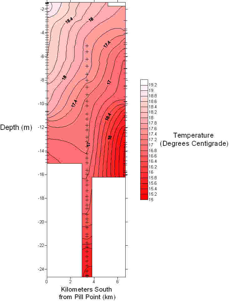 Figure 28: contour plot of temperature
Figure 29: contour plot of salinity. |
(Table 3: Table showing turbidity found in the estuary at three different sites)
|
Euphotic Depth Table 3 shows the lowest transmissometer average was found at Station 1, this is because it is closest to the riverine input which brings in sediment particulate matter causing a high light attenuation. The Secchi disc data agrees with the transmissometer data. The furthest station from the riverine input, Station 3, shows the highest transmissometer average as well as the deepest Secchi disk depth. This is because in this area most particulate matter has been mixed deeper, been scavenged or settled out of the water column so light has a lower attenuation. This allows light to penetrate deeper, increasing the euphotic zone so phytoplankton can take advantage of nutrients at greater depths where nutrients are not as depleted. |
Time Series
|
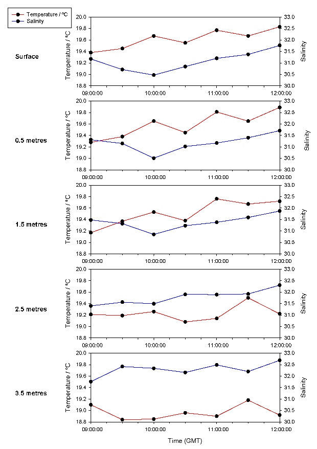
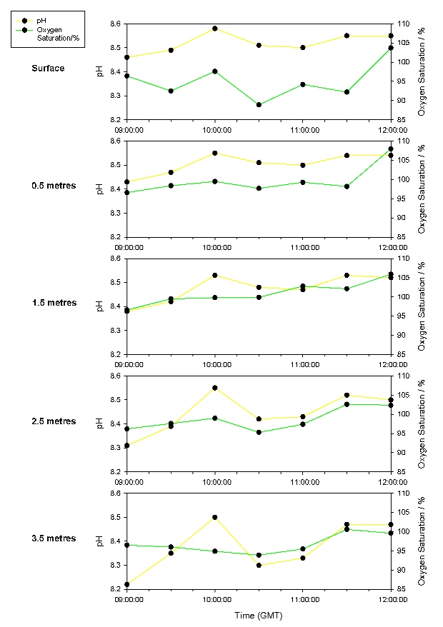
Figure 33: Time series on the pontoon of temperature and salinity.
Figure 34: Time series on the pontoon of pH and oxygen concentration. |
Figure 33 shows an overall increase in temperature throughout the time series. This is due to the heating effect of solar radiation. This effect is reduced at depth due to the attenuation of the radiation by the water column, the low heat conductivity of water, and a lack of mixing. Variation in the top 1.5 metres is due to atmospheric effects such as mixing by the wind and cloud cover. For example, the large dip from the surface to 2.5 metres at 10:30 GMT is possibly due to a prolonged period of cloud cover. The spike at 2.5 and 3.5 metres at 11:30 GMT is probably due to increased mixing of warmer surface water to depth, possibly caused by increased wind mixing. This increase is mirrored by a decrease in surface temperatures. There is an initial decrease in salinity (Figure 33) due to the effect of the ebbing tide, increasing the influence of the riverine component of the estuarine water body. However, there is an overall increase in salinity due to the effect of the flooding tide, after low water at 09:21 GMT, which carries saline water further up the estuary. This effect is delayed due to the distance of the sampling point up the estuary. The salinity at depth is higher due the high density salt water flowing under the overlying freshwater. This variation decreases over time due to the flooding tide causing increased mixing which results from turbulence caused by shear between the headward flow of saline water and the mouthward flow of river water. There is an overall increase in dissolved oxygen saturation (DOS) over time (Figure 34) from 0.5 metres to 3.5 metres due to the increase in the photosynthetic activity of phytoplankton, as confirmed by the chlorophyll time series in Figure 35. DOS at the surface is very variable due to the mixing effect of the wind and diffusion over the surface layer. DOS is lower at depth as the inputs from the atmosphere are not fully mixed to these depths and also possibly due to reduced photosynthetic activity resulting from a shallow euphotic depth caused by re-suspension of sediments resulting in high turbidity. However, it must be noted that this is hypothetical as the euphotic depth was not measured. pH (Figure) 34 increases over time due to carbon dioxide usage by phytoplankton which results in a decrease in carbonic acid as determined by the equilibrium characteristics of the reversible reaction: H2CO3 ↔ CO2 + H2O pH is also lower at depth due to hypothesized reduced photosynthetic activity.
|
|
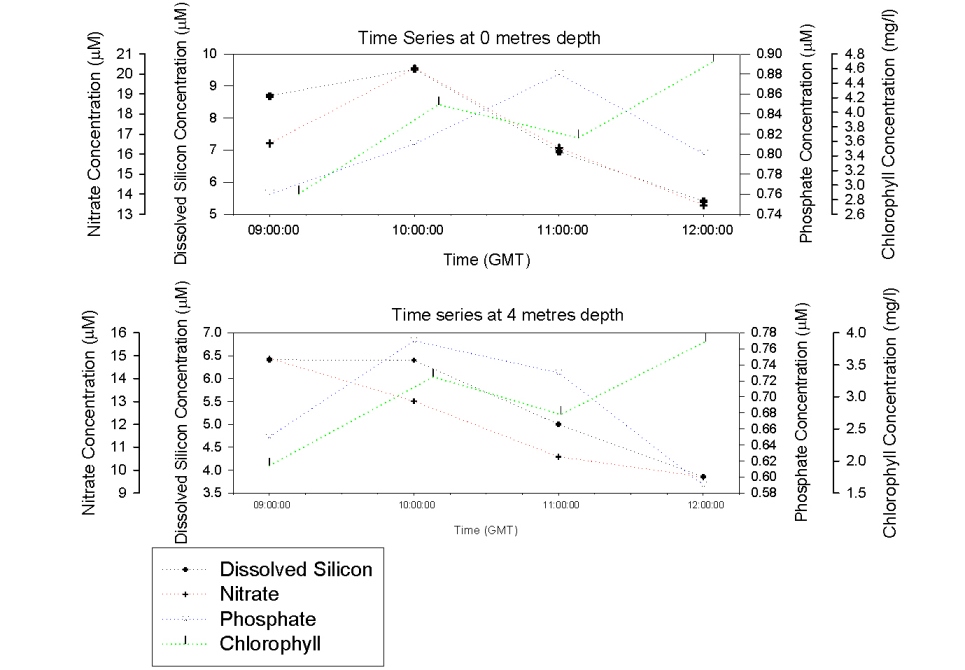
Figure 35 shows an increase in surface nitrate concentration between 9:00 and 10:00 GMT before decreasing between 10:00 and 12:00 GMT. At 4m depth the concentration decreases constantly from 9:00 -12:00 GMT. Between 9:00GMT and 12:00GMT there would be an increase in irradiance, causing an increase in phytoplankton production and therefore a decrease in nitrates from 9:00 – 12:00GMT. At both 0m and 4m depth dissolved silicon stays constant between 9:00-10:00GMT and then decreases in concentration though to 12:00GMT. This again could be due to the increase in irradiance though the morning resulting in increased removal from primary production. Phosphate results differ from nitrate and dissolved silicon in that they increase at 0 metres from 9:00-11:00 GMT and then decreases until 12:00 GMT. At 4m depth phosphate increases between 9:00-10:00GMT and then decreases until 12:00GMT. This difference is possible due to anthropogenic inputs such as the sewage outflow demonstrated in the mixing diagram (Figure 38). At both 0m and 4m depth chlorophyll concentrations increase from 9:00-12:00GMT indicating the increase in phytoplankton production. This can also be seen from the dissolved oxygen data in figure 34 showing that photosynthesis increases from 9:00-12:00GMT so more chlorophyll is generated. |
Figure 35: Time series of nutrients from the pontoon. |
Nutrient Environment
|
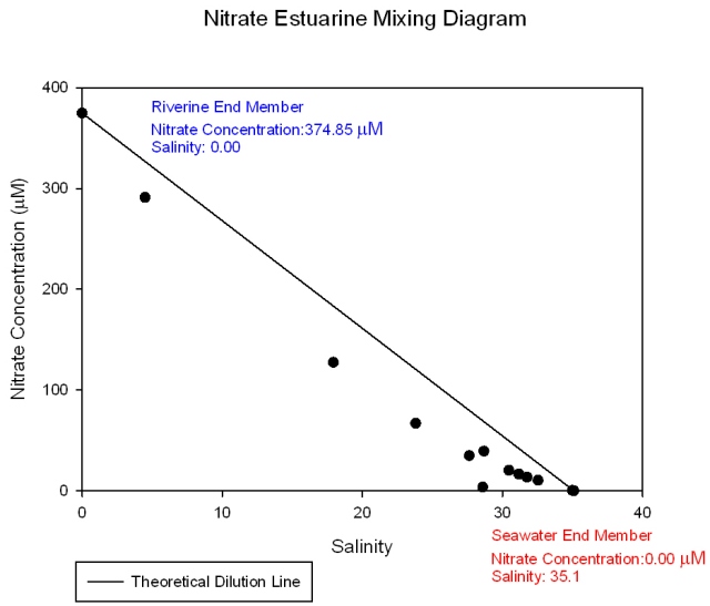
Figure 36: Nitrate estuarine mixing diagram.
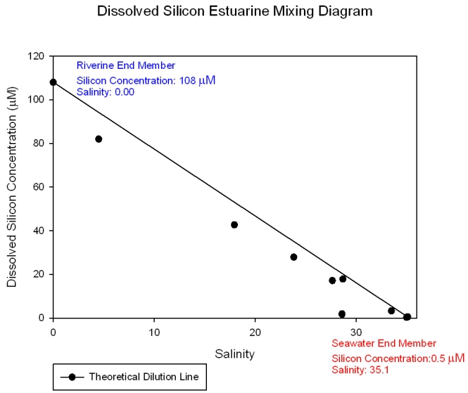
Figure 37: Dissolved silicon estuarine mixing diagram.
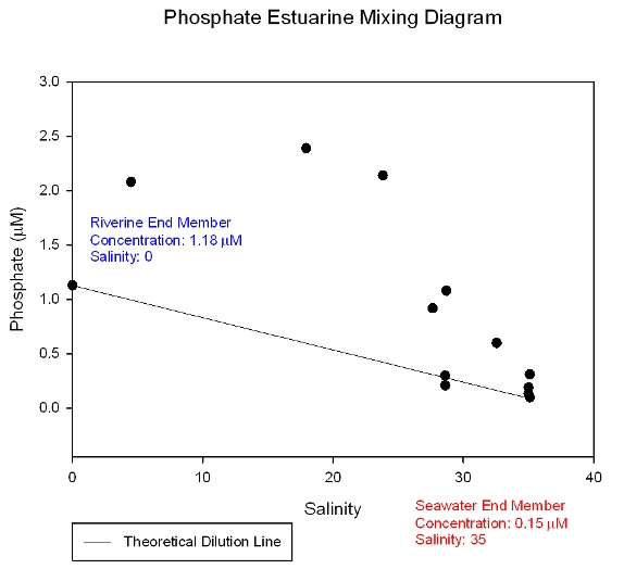
Figure 38: Phosphate estuarine mixing diagram
|
The nitrate mixing diagram (Figure 36) shows a higher concentration of nitrate at the riverine end member as expected due to nitrates being added to the estuary mainly by riverine and anthropogenic inputs such as agricultural effluents. The samples plot below the theoretical dilution line (TDL) indicating that nitrate is behaving non conservatively and is being lost from the system. This is due to biological removal. So even though there is a large anthropogenic input of nitrate the biological activity at this time of year is high enough to cause a net removal from the system. There are relatively large gaps in the data towards the lower salinity areas which may be hiding different nutrient behaviour. The dissolved silicon mixing diagram (Figure 37) shows that silicon is at a higher concentration in river water than sea water and that it behaves conservatively within the estuary as all the samples plot on or close to the TDL. This means the concentration of dissolved silicon depends entirely on the degree of mixing between fresh and salt water. However dissolved silicon is a biologically essential nutrient and may only be behaving pseudo-conservatively if the in situ rate of removal is slower than the rate of transportation through the estuary or if any addition or removal is exactly matched by corresponding removal or addition. However, it must be noted that the riverine end member replicas are not accurate and therefore the behaviour may be more conservative or become non conservative respectively depending on whether the lower or higher concentration is more accurate. Comparisons with data from other groups proved inconclusive. Phosphate (Figure 38) shows a different pattern than seen for nitrate and dissolved silicon. It still shows a decrease in concentration toward the seaward end member but the samples plot above the line showing it is behaving non-conservatively as it is being added to the system. This is because there is a large phosphate input from the sewage treatment plants which are located at Truro and the head of the Tresillian river. The riverine input value for all of these nutrients may be particularly high do to the effect of the previous days precipitation. |
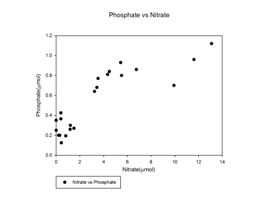
| Nutrient Limitation A plot of nitrate concentration against phosphate concentration was constructed using the corresponding concentrations from each of the 21 water samples collected. From the graph it can be seen that once nitrate has been fully depleted there is still some phosphate available. This shows that nitrate is depleted by phytoplankton before phosphate, suggesting that nitrate is the limiting nutrient within the estuary. This may be a result of the addition of phosphate to the estuary from sewage input as seen in the mixing diagram (Figure 39). |
Figure 39: phosphate vs. nitrate graph |
|
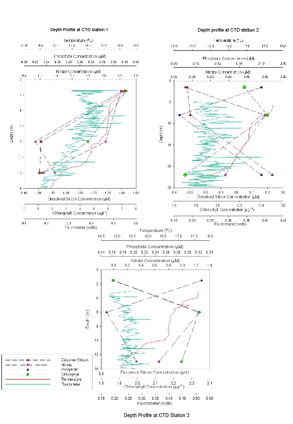
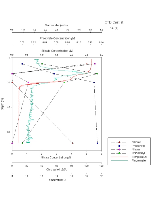
CTD Depth Profiles (Figure 40) Dissolved silicate concentrations decrease throughout the estuary from station 1-3. Dissolved silicate concentrations at Station 1 are detectable throughout the entire water column with the highest concentration (2.1 μM) at 1.5 metres, decreasing to 1.8 μM at 13 metres. At Stations 2 and 3, dissolved silicon is below detection limit or at a higher concentration at depth respectively. At Station 2 concentrations are only detectable at 22 metres where phytoplankton population and irradiance are low. Phosphate concentrations are highest at the shallow depths at all stations and are lowest at the mid sample depths. This is due to sampling taking place just after the spring bloom, so phytoplankton have depleted the nutrient concentrations. Phosphate concentrations are highest at Station 1, 0.4 μM due to high inputs of phosphate from sewage outfalls at Truro. Nitrate concentration at the surface decreased from Station 1 at the top of Carrick Roads to the mouth of the estuary at Station 3, near Black Rock, where the concentration was 0.0μM compared to 3.5μM at Station 1. Station 1 shows an overall decrease in nitrate from the surface, 3.5 μM, to 1.0 μM at 12 metres which is mimicked by the chlorophyll data. Stations 2 and 3, have a lower amount of nitrate at the surface, with increases with depth until 6-8 metres, before decreasing again. Chlorophyll trends follow the nutrient trends. It decreases from Station 1 down to Station 3, which follows the decrease in nutrients. It also shows an increase towards the middle of the water column and a decrease at depth due which follows nutrient concentrations. Station 1 is an exception with highest values at the surface. The fluorometer data from the CTD profile only shows a strong relationship with the chlorophyll values collect from water samples at Station 1. |
Figure 40: nutrient depth profiles
Secchi depth vs. actual depth. |
Phytoplankton & Zooplankton
Phytoplankton
|
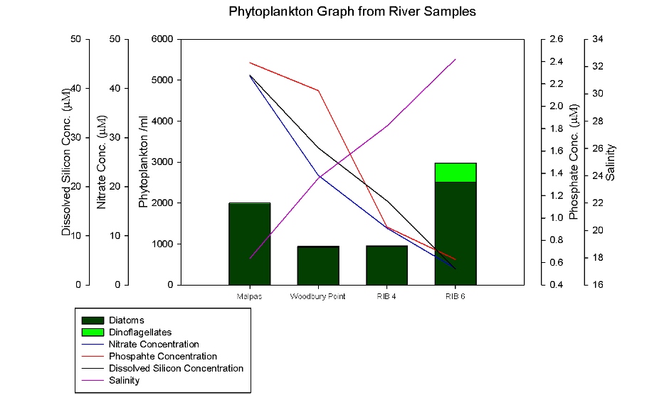
Two sets of phytoplankton samples were taken, one as a time series from the King Harry Pontoon (Figure 42) and another set taken on the RIB as it moved down the estuary (Figure 41). During the time series, there is an overall decrease in phytoplankton which is the opposite to all other indicators of phytoplankton activity including chlorophyll which increases and nutrient concentrations which decreases (Figure 35). This anomaly maybe due to different people, with varying experience, judging differently between plankton and debris and using different characteristics to identify the phytoplankton, skewing the results. Figure 41 from the RIB samples had an improved correlation for phytoplankton indicating that the amount of phytoplankton present increases down the estuary. Figure 41 and 42 show that diatoms are dominating over dinoflagellates throughout the head of Fal Estuary and Truro River. 90% of the diatoms are made up of diatom chains, such as Chaetoceros sp, with a very small amount of centric diatoms, Coscinodiscos sp., and an even smaller amount of pennate diatoms, Rhizosolenia sp, in all the samples. Dinoflagellates were absent at lower salinity samples taken higher up the river. The sample taken at Malpas, on the Truro River has the highest concentration of chlorophyll, phosphate (P), nitrate (N) and silicate (Si) which could be due to the close proximity to the sewage outfalls at Truro and on the Tresillian River. It has the lowest salinity of any sample taken and is dominated by diatoms. Diatoms thrive in water with high nutrient concentrations possibly explaining why they can outcompete the dinoflagellates. At RIB Station 6 there is an increase in the amount of phytoplankton overall, especially in the dinoflagellate Alexandrium sp., which can cause toxic algal blooms. This increase may be due to a counting error or the presence of a different nutrient environment. |
Figure 41: To show phytoplankton from the RIB river samples
Figure 42: To show phytoplankton from the pontoon river samples |
Zooplankton
|
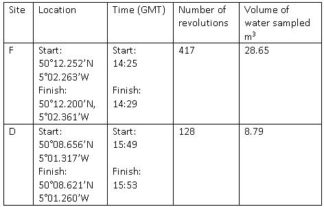
Zooplankton trawl data for both sites |
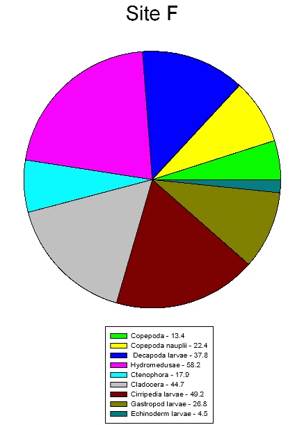
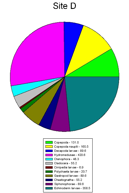
Zooplankton samples were collected from two sites in the estuary using a 200µm plankton net with a 54cm diameter opening. Site F was located just off Turnaware Point, at the head of Carrick Roads and site D was just off St Anthony Head, at the mouth of Carrick Roads. |
|
The sites show differences in zooplankton abundance mainly due to differences in nutrients. A total of 43 organisms were found in the first sample and 18 organisms found in the second sample at site F (Figure 43). This is less than the total number of organisms found in each sample at site D (Figure 44), which was 114 and 111. Site F shows a higher concentration of nutrients (Table 4) than site D because it is closer to the river input. The most dominant zooplankton found at site F were hydromedusae, cirripedia larvae and cladocera. These three are all filter feeders and therefore need a high abundance of food resources in the water column to thrive. At this site there are high nutrient concentrations and lots of detritus in the water column inflowing from the river providing a perfect environment for these species. Site D shows the most dominant zooplankton being echinoderm larvae and hydromedusae. Here cladocera and cirripedia larvae abundance is low, this could be due to the drop in nutrients in the water column. Hydromedusae populations are high at both sites, this is because in their polyp form they are filter feeders so thrive in high nutrient environments but in their medusae form they are predators so are able to survive in relatively lower nutrient environments. |
Table 4: Nutrient concentrations at both zooplankton trawl sites.
|
Calibration Curves
 |
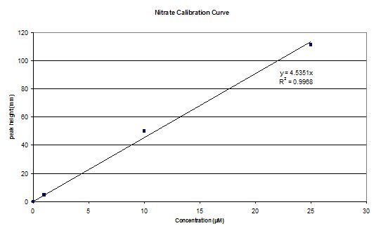 |
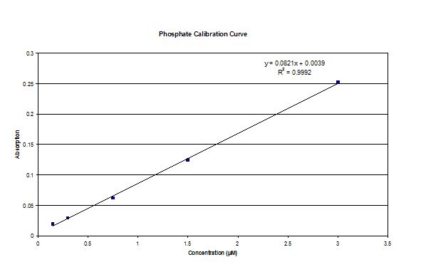 |
| Dissolved Silicon calibration curve | Nitrate calibration curve | Phosphate calibration curve |
|
Summary |
The ADCP data collected confirmed the estuary was partially/well mixed depending on the spring neap cycle and showed asymmetrical circulation throughout. An increase in oxygen concentration down the estuary was found which is a possible result of eutrophication in the upper estuary. Sewage outflows from the two sewage plants have a positive effect on the levels of phosphate which is characteristic of a polluted estuary; this is also seen by the non conservative behaviour of phosphate which is being added to the estuary. Nitrate shows a non conservative behaviour and is being lost from the system, while silicon shows conservative behaviour; this reflects the typical behaviour of these nutrients within many estuaries.
The relationship between nutrients and phytoplankton is complex with some contradictory trends such as both nitrate and chlorophyll increasing with depth. Further research must be completed to confirm the reasons behind these trends or to indicate if they have been caused by errors in the analysis.
The majority of the changes seen are due to the effects the tide has on the estuary though out the day.
![]()
![]()
![]()
![]()
![]()
![]()
| Aim |
To explore the physical, chemical and biological interactions occurring in stratified waters 9.5 nautical miles SE off the coast of Falmouth and how these interactions change over a time series.
|
Introduction |
On 08/07/09 RV Callista was taken offshore outside the Fal Estuary to gather biological, physical and chemical parameters in the stratified water column. A time series was gathered at a single location , in addition to a data set collected at the mouth of the estuary at Black Rock. At the offshore station, data were collected half-hourly to create a time series of CTD profiles. Water Samples were taken every hour at three different depths for on-shore analysis of dissolved oxygen, chlorophyll, phytoplankton and nutrients. A closing zooplankton net was used every hour opened between 20-10 meters, to sample through the chlorophyll maximum and thermocline.
|
Weather
|
Tides
|
| Methods |
At Black Rock, a complete CTD data set and water samples were collected at 08:00 GMT. Offshore, at the second station, data were collected half-hourly from 09:30 to 15:00 GMT. The CTD was lowered and the data was captured during the descent was presented on screen in real-time. Five niskin bottles were used to collect samples hourly at various depths in the water column. A closing phytoplankton trawl net (200um mesh, 500ml bottle) was deployed every hour between 20-10 meters. An ADCP was used to measure the current flow throughout the day, as well as identifying areas of high zooplankton abundance.
| Results - Black Rock |
|
Figure 45: ADCP data from Black Rock station. |
This transect (Figure 45) was taken at Black Rock. Starting at 50o 08.777 N, 05o 01.484 W, at the centre of the mouth of the estuary (approximate depth of 31 metres), the vessel moved SSE towards the shore (approximate depth of 17 metres). The current is strongest near the surface with velocities up to 0.3ms-1. Between 8 and 10m the current slows to approximately 0.1ms-1 which will result in significant shear and is then constant with depth. In the deeper water below 20m the current direction is variable between 180o and 300o resulting in some shear. Otherwise the current direction is fairly homogeneous. There is significant backscatter at 10m which indicates a large amount of zooplankton is present. |

|
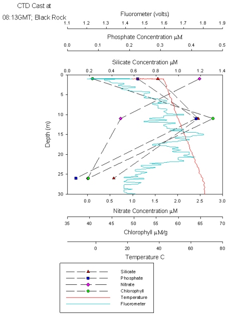
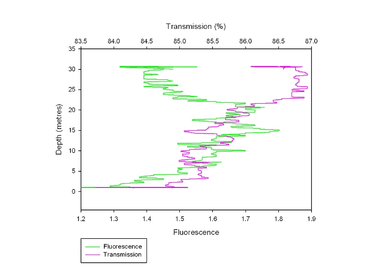
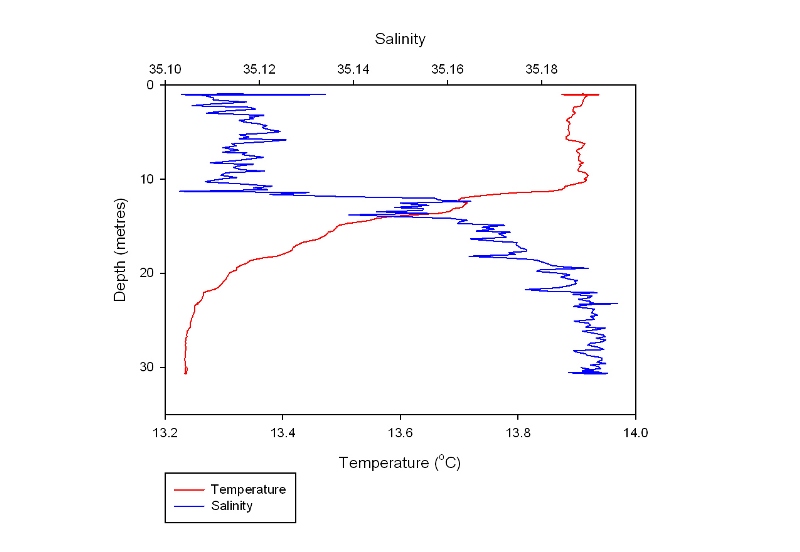
This station follows the nutrient depth profiles seen in the estuary and shows a similar pattern to Plot 3 from the estuarine nutrient depth profiles. All nutrients peak below the surface at 12m (Figure 46) just above a weak thermocline. Chlorophyll corresponds to this peak, and nitrate decreases constantly down the water column. This graph shows the water column is well mixed with only small change in temperature with depth. Temperature The temperature (Figure 48) remains relatively constant at 13.9°C down to 10 metres. There is then a thermocline where the temperature drops down to 13.2°C at 24 metres. The temperature then remains constant again down to the bottom at 31 metres. The thermocline is weaker than that recorded offshore as the waters are less stratified. Salinity The salinity (Figure 48) also shows two distinct, homogenous layers. The upper layer has a salinity of 31.1 and is present down to 11 metres. There is then a halocline where the salinity changes to 35.2 in the lower layer, which starts at 19 metres. This is due to the presence of the thermocline, which prevents inputs of fresh water (for example from rain) from mixing into the lower layer. Fluorometer The fluorescence (Figure 47) at the surface is 1.4 volts it then increases to a maximum of 1.8 volts at 15 metres. This is due to the depth of the euphotic zone being 17 metres (Table 6) and so below this there is insufficient light for photosynthesis. However, the fluorescence doesn’t return to the surface level of 1.4 until 26 metres. This is due to the phytoplankton being mixed down below the euphotic zone but not beyond the thermocline. Transmission The percentage transmission (Figure 47) is relatively low at the surface (84.8%) before increasing to 85.8% at 12 metres, suggesting that the surface has quite a high turbidity as this increase cannot be explained by the fluorescence levels. The transmission then dips down to 85.1% at 15 metres, matching the peak in the fluorescence data. It then increases again to a maximum of 86.8% at 26 metres, again matching the fluorescence data. Below 26 metres, the transmission stays relatively constant. |
Figure 46: nutrient depth profile at Black Rock
Figure 47: Transmissometer and fluorometer depth profile
Figure 48: temperature and salinity profile |
|
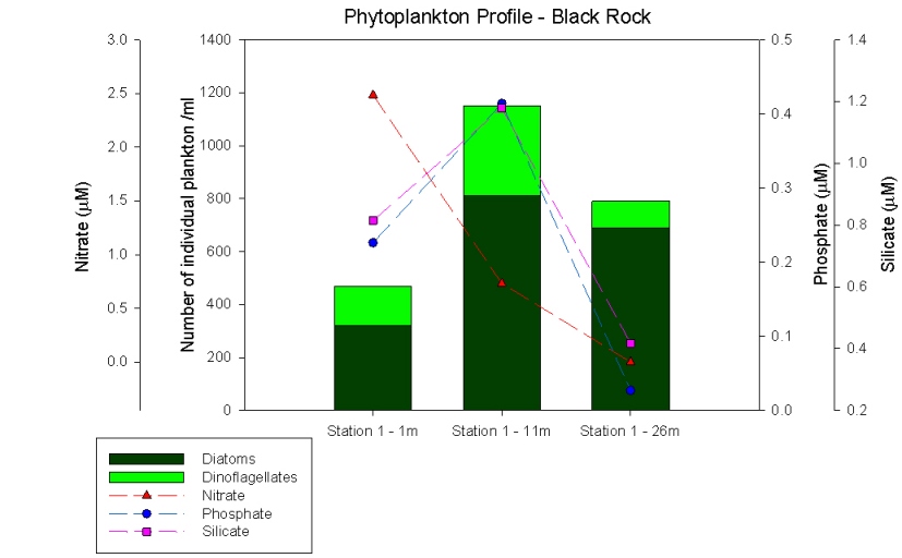
Figure 49: phytoplantkton profile for Black Rock. |
Black rock phytoplankton profile (Figure 49) follows on from the estuary data and shows a increase in the amount of dinoflagellates present. There is the highest amount of plankton at 11m which correlates with the thermocline and chlorophyll maxima shown in figures 47 and 48. There are more diatoms than dinoflagellates as silicate concentrations are still high and they can outcompete dinoflagellates. The main species of dinoflagellates present are Karinia Mitimotoi which are characteristic of themoclines, compared to the Alexandium sp. found in the estuary. After the 11m the nutrients are rapidly depleted. |
|
Time Series |
|
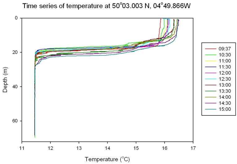
Figure 50: time series of temperature |
Temperature: Figure 50 All depth profiles show a well defined thermocline at around 17 metres. For example, at 10:30 GMT the temperature drops from 15.8°C at 13 metres to 11.5°C at 19 metres. Later in the day the thermocline becomes less abrupt and migrates downward through the water column. For example, at 15:00 GMT the water temperature dropped from 16.4°C at 12 metres to 11.5°C at 27 metres. |
|
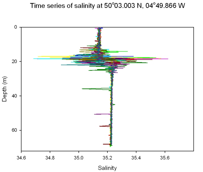
Salinity: Figure 51 Salinity is relatively homogenous throughout the water column, although it is separated into a two layer system by a slight halocline around the same depth as the thermocline (18 metres). For example, at 09:37 GMT it is 35.1 at 15 metres and 35.2 at 22 metres. This is too significant a change to be caused just by recent rainfall and is due to a build up of the freshwater input over a prolonged period of time caused by the prevention of mixing of the fresher water into the lower layer by the thermocline. The salinities of the upper and lower layer stay constant throughout the day. Salinity spikes occur around the depth of the thermocline. This is due to the difference in the refresh rates of the temperature and conductivity instruments which causes salinity to be miscalculated. |
Figure 51: time series of salinity |
|
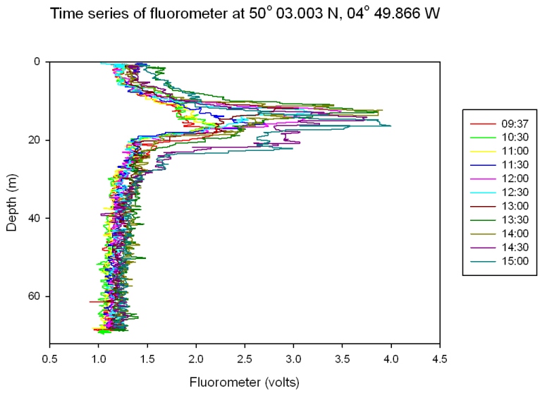
Figure 52: time series of fluorescence |
Fluorescence: Figure 52 The fluorescence shows a significant increase from around 1.4 volts at the surface to a maximum of between 2.2 and 4.4 volts. This maximum is present between 13 metres at 13:00 GMT and 16 metres at 15:00 GMT throughout the day. This represents a high chlorophyll concentration which in turn demonstrates a large phytoplankton population just above the level of the thermocline. This is because the nutrient levels in the surface waters are depleted after the spring bloom but there are nutrients being mixed up from below the thermocline, allowing phytoplankton growth. The reason this growth isn’t deeper is because the thermocline prevents mixing of phytoplankton into the lower layer, even though for most of the day the euphotic zone is deeper and so photosynthesis could occur below this depth (as shown in Table 6). Up until 14:30 GMT fluorescence drops back to the surface value of 1.4 below 21 metres. At 14:30 and 15:00 GMT this deepens to 26 metres suggesting chlorophyll is being mixed downwards. |
|
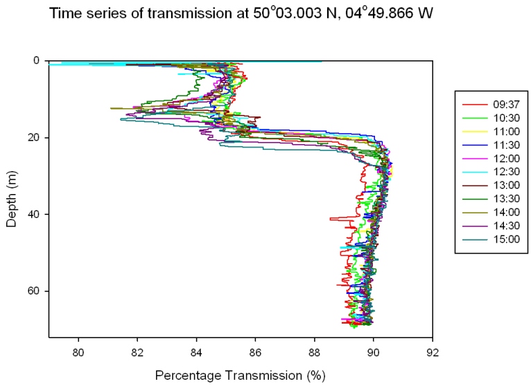
Transmission: Figure 53 The percentage transmission is relatively low in the upper layer of the water column and drops to a minimum between 11 and 15 metres. For example, at 14:00 GMT the percentage transmission is only 81.1% at 12 metres. This is due to phytoplankton in the water column causing greater light attenuation, reaching a maximum at the chlorophyll maximum around 15 metres, as shown by the fluorometer. The transmission then increases again until around 21 metres throughout most of the day, for example at 10:30 GMT, although this also deepens to 26 metres at 14:30 and 15:00 GMT, corresponding with the deepening chlorophyll maximum. |
Figure 53: time series of tranmission |
|
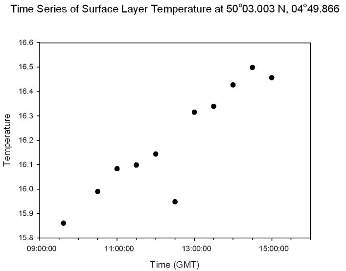
Figure 54: time series of surface temperature |
Surface Layer Temperature: Figure 54 The surface layer temperature increases steadily throughout the day from 15.9°C at 9:30 GMT to 16.5°C at 15:00 GMT. There is a slight dip at 12:30 GMT where the temperature drops down to 15.9°C from 16.1°C at 12:00 GMT. This is either due to the instrument misreading slightly or atmospheric effects, such as increased wind speed or prolonged cloud cover. |
Depth Profiles
|
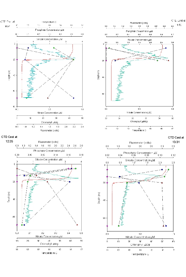
Figure 55: nutrient depth profiles
Figure 56: nutrient depth profiles, part 2.
Figure 57: nutrient time series. |
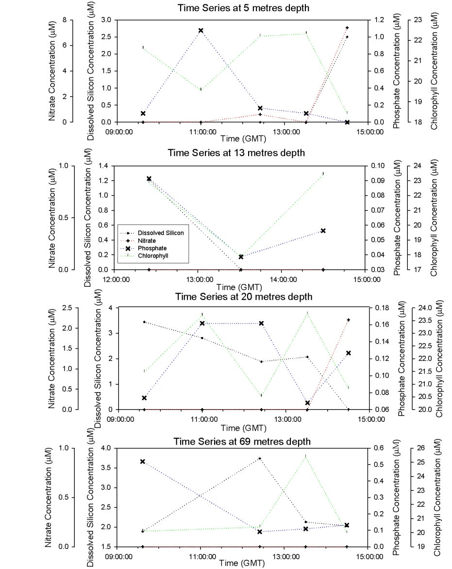
The plots show 5 different CTD casts (Figures 55 and 56), the first at 9.13 is at Black rock outside the Fal Estuary and is a continuation of the estuarine plots. The rest are a time series at a offshore point 50’03.424N 04’49.903W. The graph for 11.37 has only two points as bottles failed to close at 67m. Figure 57 shows a time series at offshore station for each depth. Time Series 9:37 – 14:30: Figures 55 and 56 Nitrate concentrations are below detection at nearly every depth sampled at every station; this is because it is constantly being utilized by phytoplankton and is limiting growth. There are small peaks at the surface at CTD casts 12.25 and 14.30, but shows no pattern. Phosphate shows a constant pattern of increasing from the surface to the thermocline and then decreasing down to depth. This is because nutrients are concentrated at the thermocline by being mixed up from deeper water. Silicate profiles generally increase at the thermocline from 0.0 µM to above 2µM throughout the time series but show no definite pattern to greater depth. The last time series is the only exception with high concentrations at the surface and lower concentrations at the thermocline. This could be due to different types of plankton migrating to the thermocline at different times of the day which use silicate e.g. diatoms. The chlorophyll data correlates with the fluorometer accurately and in one case follows it exactly. The chlorophyll maximum always peaks when there is a high concentration of at least one or more main nutrients. The chlorophyll maxima and thermocline always appear above 20m with the chlorophyll maxima getting higher throughout the day and the thermocline migrating slightly deeper as it is thermally heated. The nutrient concentrations are far lower offshore than in the estuary this is due to the low input of nutrients to the water. Depth Time Series (09:37- 14.30) Figure 57 shows a time series for each nutrient at each depth to show clearly how each nutrient changes over time at each depth. Nitrate concentration is below detection at most stations as mentioned for figure 55 and 56 above. Nutrient concentrations at each depth don’t show any general patterns or trends, some decrease throughout the day while some increase. Between 13.14 and 14.30, at every depth, there is a decrease in chlorophyll which maybe caused by a vertical migration of plankton. Phosphate and silicate are usually depleted by this point as well, except at 5m where there is large increase in phosphate. There are also peaks in nitrate at 5m and 20m depth. |
ADCP
|
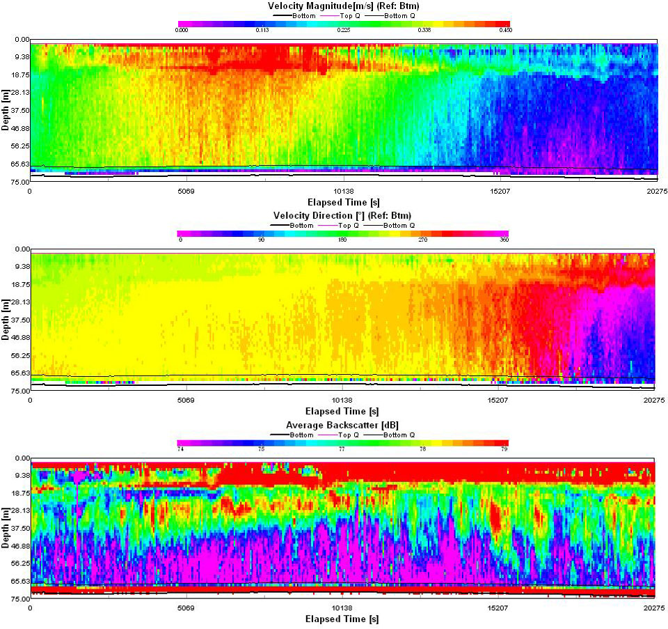
An ADCP profile (Figure 58) was taken throughout the duration of the time series. The velocity magnitude and direction is dominated by the channel tidal regime throughout the profile. At the start of the profile the current (approx. 0.3ms-1) is flowing out of the channel with the ebbing tide on a bearing of 245o. As low tide is approached (12:20 GMT at Falmouth) the current speeds up and begin to swing round in a clockwise direction, passing though north until eventually at the end of the profile the current direction is now into the channel with the flooding tide on an angle of 90o. The highest current velocity is found around the time of low tide (approx 0.45ms-1) before then decreasing with the flooding tide to its lowest value in the profile around 0.1 ms-1. There is a constant high backscatter at 30m at the start of the day which slowly rises throughout the day to 15m indication a possible upward advection of zooplankton. The high backscatter between 10 and 20 meters indicates high abundances of zooplankton and subsequently it was this depth range that was sampled with the closing net. The very backscatter at the very surface is likely to be noise caused by for example the anchor chain or surface bubbles. |
Figure 58: ADCP data. |
Richardson's Number and Brunt-Vaisala Frequency
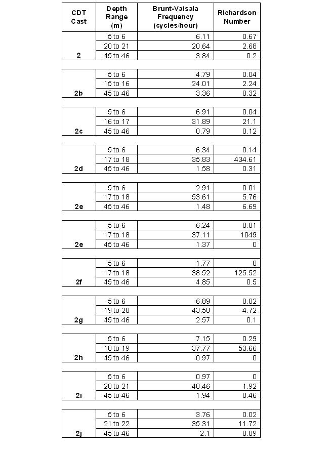 Table 5: Richardson's number and Brunt-Vaisala frequency |
The Richardson Number and Brunt-Vaisala Frequency (Table 5) were used to quantify the extent of density stratification and mixing for each CTD profile collected in the time series. A Richardson Number below 0.25 indicates the presence of shear instabilities such as Kelvin – Helmoltz billows whilst a value greater than 1 indicates laminar flow (no mixing). Values for each parameter were calculated over one metre intervals in the upper mixed layer (5 to 6 m), over the thermocline (varying depths) and in the lower mixed layer below the thermocline (45 to 46 m). All the values except one follow the expected pattern with low Brunt-Vaisala Frequencies and Richardson Numbers less than 0.25 above and below the thermocline, with high values within the thermocline itself. The low values found above and below the thermocline are indicative of the weak density stratification and high shear found in these areas. This results in turbulent mixing and hence the straight lines of temperature and salinity as seen on the CTD depth profiles (Figures 50 and 51). Within the thermocline the values are larger and all Richardson Numbers are above 1. This is caused by the increase in density stratification stabilising the water column overcoming the effects of shear and therefore reducing the extent of turbulent mixing. The high Brunt-Vaisala Frequency is a result of the strong density stratification causing a high natural oscillation rate of internal waves. At station 2e the lower mixed layer Richardson Number is particularly high with a value of 6.69. This is most likely not a representative value for the entire region and only arose because the difference in velocity magnitude between 45 and 46 metres was 0.001 ms-1 resulting in very little shear. |
Euphotic Depth: Table 6
| The CTD used in the offshore work contained a log light meter to enable calculation of the euphotic depth. The euphotic depth is the depth of the 1% light level. It can be seem from Table 6 that the euphotic depth off shore is greater than that of black rock and in the estuary (Table 3). This is due to there being much suspended particulate matter within the water column to attenuate the light. Over the time series (each time in the table refers to the time of a CTD cast) the euphotic depth remains relatively constant with a few anomalies such as 09:37 and 13:30. The high value at 09:37 could have been caused by instrument instability whilst the drop at 13:30 could have been caused by increased cloud cover if the instrument did not factor in surface irradiance. |
|
Phytoplankton
|
Figure 59 shows a phytoplankton profile at the first CTD cast (Station 2, 9:13 GMT) and the last CTD cast (Station 9, 14:30 GMT). There is a greater amount of growth in the surface layer at station two with a large percentage of diatoms over dinoflagellates as diatoms prefer the higher irradiance at the surface. At depth the dinoflagellates show dominance as they prefer the lower irradiance at the thermocline. By 67 metres there are low amounts of phytoplankton due to no light and low levels of nutrients except for an accumulation of phosphate. Station 9 shows a greater dominance of dinoflagellates due to the low levels of silicate and nitrate limiting diatom growth, there is also a far greater concentration of plankton per ml rising from 340/ml at 20 metres (Station 2) to 840/ml at 20 metres (Station 9) and 2040/ml at 13 metres. Also, there was an increase in nitrate concentration compared to the depleted source at Station 2. The main difference between the offshore and estuary samples are the ratios between diatoms and dinoflagellates and the species present. In the estuary diatoms were 90% diatom chains, where as offshore they are mainly centric e.g. Coscodiscus. The main dinoflagellates present were Alexandrium sp in the estuary where as the main species present offshore had a variety including Karina mikimotoi, Dinophysis and Polykrikos. Diatoms dominate in the estuary due to the high turbulence, nutrient levels and cool water. Dinoflagellates thrive offshore with low nutrients, and less turbulence as they can outcompete the diatoms once silicate is depleted. |
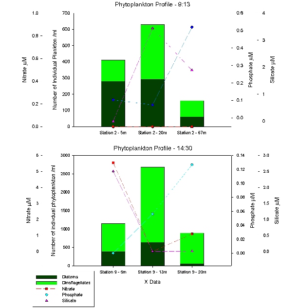 Figure 59: phytoplankton time series. |
Zooplankton
 |
 |
 |
 |
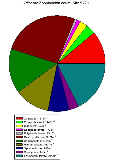 |
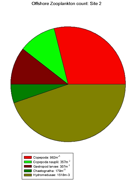
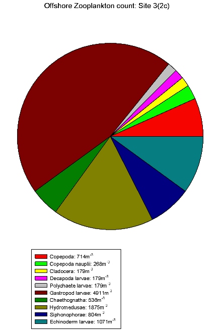
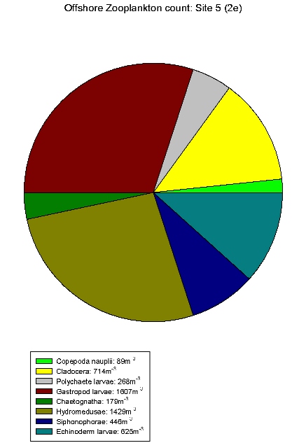
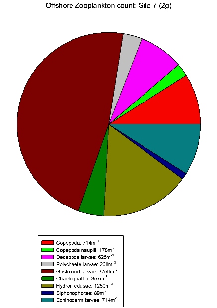
| Zooplankton count at Site 2 | Zooplankton count at Site 3 | Zooplankton count at Site 5 | Zooplankton count at Site 7. | Zooplankton count at Site 9. |
|
|
|
Gastropod larvae make up a large proportion of sites 3(2c), 5(2e), 7(2g) and 9(2i), these sites show a lower equitability than Site 1. Hydromedusae make up a large proportion of the communities of sites 2, 3(2c) and 5(2e). The high abundances within these species indicates favourable conditions in the water column at this time of year for hydromedusae and gastropod larvae.
These results differ from the
estuarine results in that gastropod larvae are only found in
relatively low abundance in the estuary. Although hydromedusae
still seem to be dominating. This could be due to gastropods
not being able to tolerate variation in salinity.
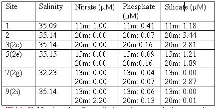
Table 7 shows offshore salinity
remained relatively constant, ideal conditions for gastropod
larvae.
|
Summary |
The ADCP data shows that the characteristics of the offshore current velocity and direction are determined by channel tidal regime. The time series showed a permanent thermocline, with the surface temperature became warmer throughout the day. A chlorophyll maximum was found throughout the day representing a large phytoplankton population just above the thermocline. Compared with the data from estuaries nutrient concentrations are relatively lower with nitrate being below detection level at nearly every site surveyed. Phytoplankton populations differ between the estuary and offshore with dinoflagellates rather than diatoms dominating offshore. Also a larger variety of zooplankton was found offshore compared with the estuary with the dominant zooplankton being gastropod larvae and hydromedusae.
![]()
![]()
![]()
![]()
![]()
![]()
In conclusion the work throughout the field course has provided a holistic overview to the interactions between the physical, biological and chemical characteristics within the Fal estuary and offshore. Interactions within the Fal estuary itself depend very much on local conditions such as tides and weather with anthropogenic factors such as sewage inputs having a significant impact in many areas. An example is the continuous addition of phosphate throughout the estuary as seen on its estuarine mixing diagram.
Further offshore the interactions are dominated by the physical environment which controls the rate and location of primary production through the processes described by the critical depth theory. The physical conditions were shown to constantly change throughout the day accompanied by the expected changes in the biology and chemistry.
Overall further work must be completed to verify our findings and ensure that our results are simply not a snapshot of a complicated and constantly changing environment.
![]()
![]()
![]()
![]()
![]()
![]()
-
Bedlerson, R.H., Kenyon, N.H., Stride, A.H. and Stubbs, A.R. 1972, Sonographs of the Sea Floor, Elsevier, pp. 144-145.
-
Birkett, D.A., Maggs, C.A. and Dring, M.J. 1998, ‘Mearl (volume V)’, An overview of dynamic and sensitivity characteristics for conservation management of marine SACs, Scottish Association for Marine Science, UK Marine SACs Project, pp. 116.
-
Bryan, G.W. and Langston, W.J. 1992, ‘Bioavailability, accumulation and effects of heavy metals in sediments with special references to United Kingdom estuaries a review’, Environmental Pollution, 76, 89-131.
-
Fal and Helford Management Forum, Fal and Helford: Marine Special Area of Conservation Management Scheme, Fal and Helford SAC Management Scheme, 2006, pp. 8-15
-
Grasshoff, K., Kremling, K. and Ehrhardt, M. 1999, ‘Methods of seawater analysis’, 3rd ed, Wiley-VCH
-
Hall-Spencer, J.M. and Moore, P.G. 2000, ‘Scallop dredging has profound, long-term impacts on mearl habitats’, ICES Journal of Marine Science, 57, 1407 – 1415.
-
Holt, T.J., Rees, E.I., Hawkins, S.J. and Seed, R. 1998, ‘Biogenic Reefs’, An overview of dynamics and sensitivity characteristics for conservation management of marine SACs, Scottish Association for Marine Science, UK Marine SACs Project, pp. 169.
-
JNCC Fal and Helford SAC Site details, [online], Available: http://www.jncc.gov.uk/protectedsites/sacselection/sac.asp?EUCode=UK0013112 [accesses 2009, July 3rd].
-
Johnson, K. and Petty, R.L. 1983, ‘Determination of nitrate and nitrite in seawater by flow injection analysis’, Limnology and Oceanography, 28, 1260-1266.
-
Langston, W.J., Chesman, B.S., Burt, G.R., Hawkins, S.J., Readman, J. and Worsfold, P. 2003, Site Characterisation of the South West European Marine Sites: Fal and Helford cSAC, Marine Biological Association, Plymouth.
-
Langston, W.J., Chesman, B.S., Burt, G.R., Taylor, M., Covey, R., Cunningham, N., Jonas, P. and Hawkins, S.J. 2006, ‘Characterisation of the European Marine Sites in South West England: the Fal and Helford candidate Special Area of Conservation (cSAC)’, Hydrobiologia, 555, 321-333.
-
Parsons, T. R., Maita, Y. and Lalli, C. 1984, ‘A manual of chemical and biological methods for seawater analysis’, Pergamon, pp173
-
Pirrie, D., Power, M.R., Rollinson, G., Hughes, S.H., Camm, G.S. and Watkins, D.C. no date, Mapping and visulisation of the historical mining contamination in the Fal Estuary,
Cornwall, [online], Available: http://projects.exeter.ac.uk/geomincentre/estuary/Main/intro.htm [accessed 2009, July 3rd]. -
Tides and Weather: www.bbc.co.uk/weather/coast/tides/southwest
-
Wilson, S., Blake, C., Berges, J.A. and Maggs, C.A. 2004, ‘Environmental tolerances of free-living coralline algae (maerl): implications for European marine conservation’, Biological Conservation, 120, 283-293.
-
Plankton net: www.rickly.com/as/images/PLANKTON.jpg
-
Secchi disc: www.dipin.kent.edu/images.Secchi%20Disk.jpg
-
SV Xplorer: http://www.fdmarine.com/userimages/1%20(2).jpg
.jpg)
All diagrams, photos etc. produced by students mentioned above unless otherwise stated.
![]()
![]()
![]()
![]()
![]()
![]()
![]()