Falmouth Field Course 2009
Group 1
![]()
|
|
Falmouth Field Course 2009 Group 1 |
|
|
|
||||
|
Jimmy Willcox Timothy Hore Kerrith Barrington-Cook Hannah Young Jennifer Fookes |
 |
Sacha Neill Julie Knott Edward Westwood Danny Devereaux Anna Cunnington |
||
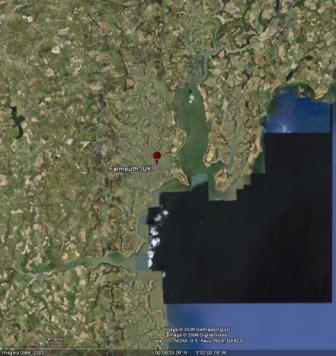 |
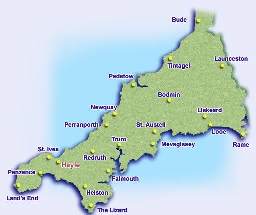
Background Falmouth Estuary, located on the SW coast of the UK, has a significant biological and socio-economic importance which has resulted in its recent European designation as a Special Area of Conservation (SAC). Made up of large shallow inlets, bays, saltmarshes, intertidal mudflats and sub-tidal sandbanks, the Fal’s physical diversity supports a myriad of marine plants and animals such as the rare Shore Dock, Rumex rupestris and maerl beds (http://www.jncc.gov.uk/protectedsites/sacselection/sac.asp?EUCode=UK0013112). Human pressures however, particularly from tin and copper mining within the Fal catchment, has put huge environmental pressures on the area since the 18th Century and has resulted in significant changes in the chemical and biological make-up of the region (Langston et al., 2003). Increased partnerships between industry and environmental organisation such as Natural England have allowed more comprehensive management of the region however, despite this Falmouth Estuary remains the most polluted estuary in the UK. |
|||||||||
|
||||||||||
|
Aims The aim of this research is to create a multidisciplinary snapshot of the Falmouth Estuary extending from the creeks which feed the system to the offshore marine environment. Biological, chemical, physical, and geological data will be collected over the two weeks to generate an inclusive overview of the system allowing investigations to be carried out on the interactions within the system. This data can be used in conjunction with previous year’s research carried out by Southampton University as well as long-term data collected by Plymouth Marine Laboratories to enhance our understanding of coastal processes with the Western English Channel. |
|||||||||
|
||||||||||
|
|
|
|||||||||||||||||
|
|
|
|||||||||||||||||
|
|
|
|||||||||||||||||
|
|
|
|||||||||||||||||
|
|
|||||||||||||||||||
|
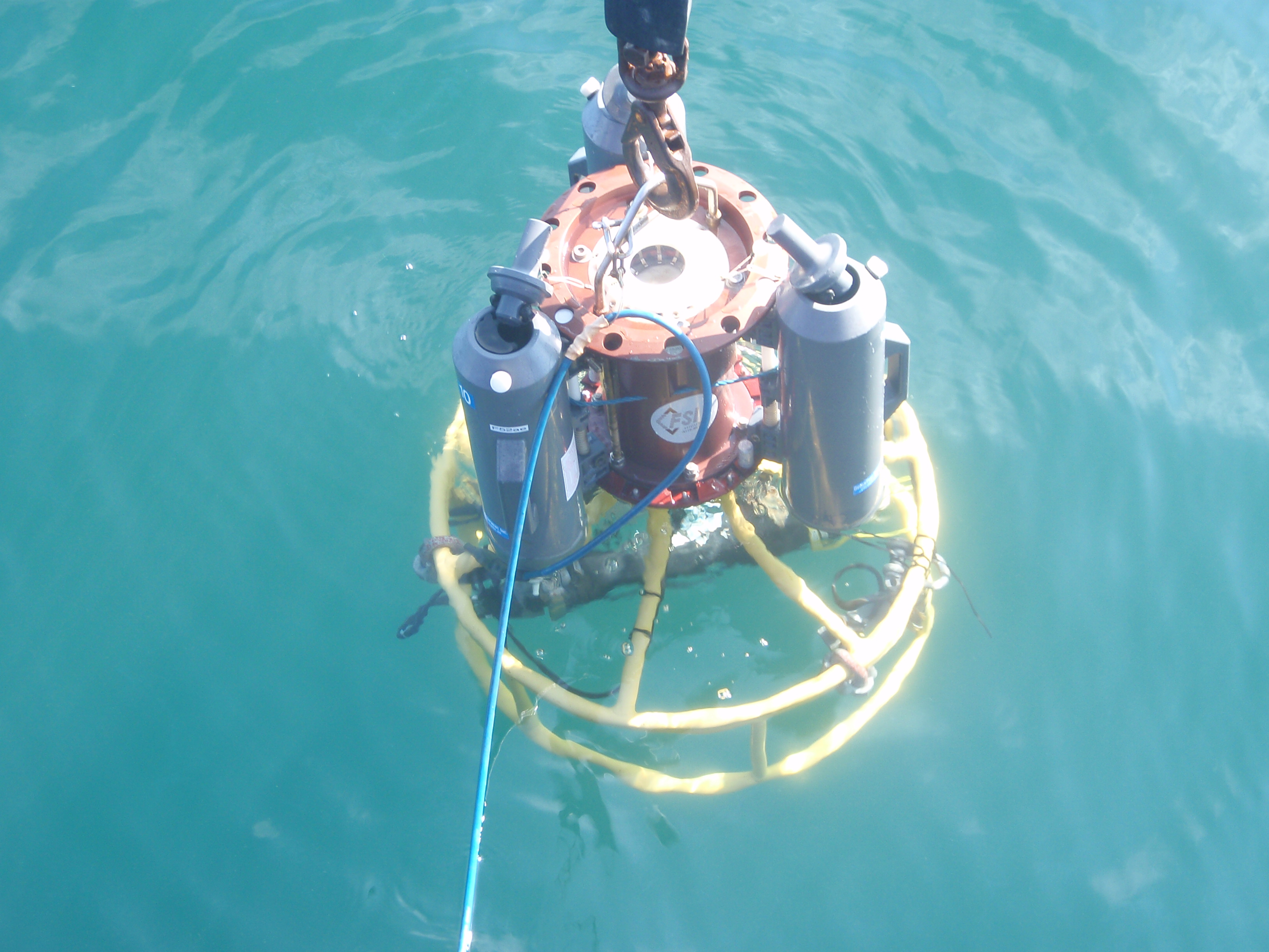
CTD + CTD Rosette |
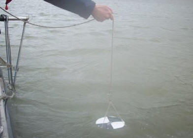
Secchi Disc |
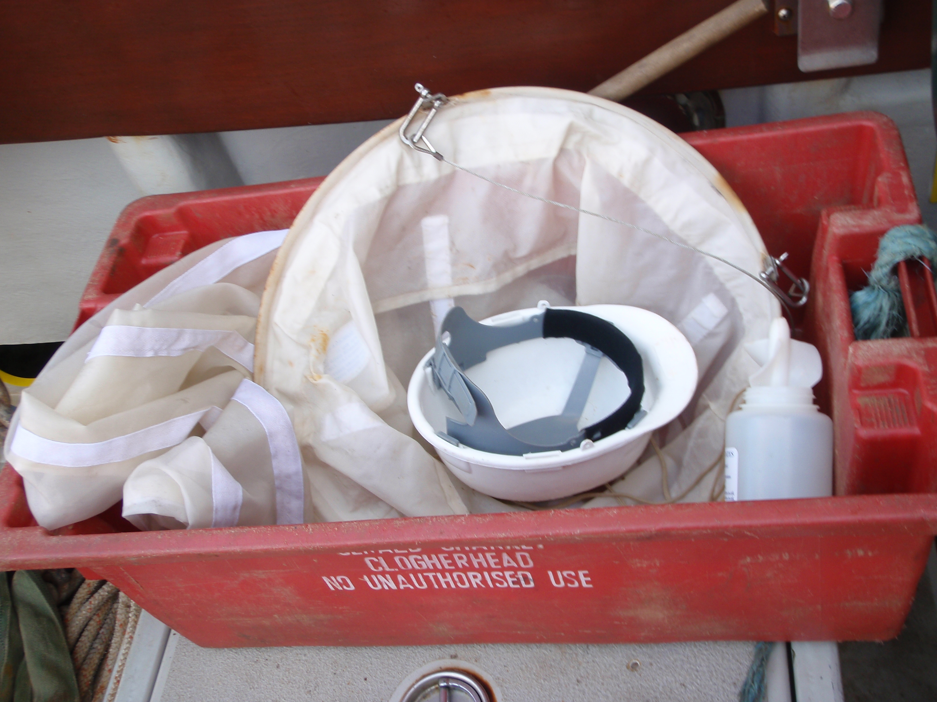
Close plankton net | ADCP | Bongo Net |
 |
|
|
 |
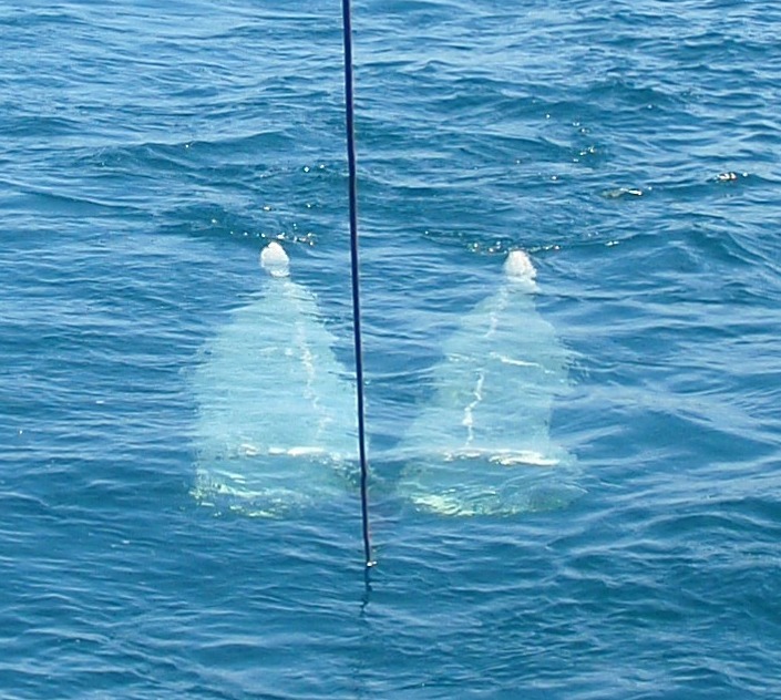 |
| Fig 3:1 CTD Rosette being lowered into the water | Fig 3:2 Secchi disc being lowered | Fig 3:3 Plankton net in a box | Fig 3:4 ADCP on steel rigging | Fig 3:5 Bongo Nets being towed |
|
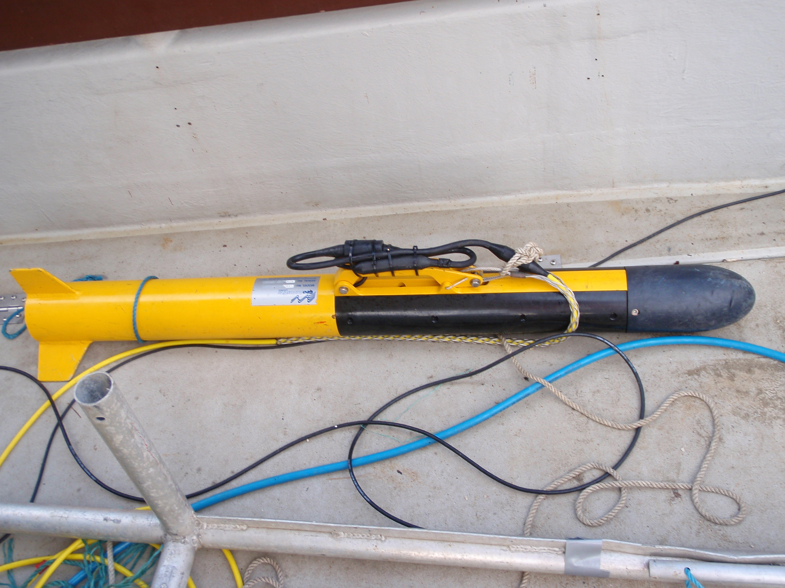
A CTD- Conductivity, Temperature, Depth profiler is used to investigate the vertical structure of the water column. It works by taking continuous recordings of salinity, temperature and depth as it is lowered through the water. Salinity is measured through the conductivity of the water passing between two charged plates. The CTD is mounted onto a Rosette together with a fluorometer and Niskin bottles which could be closed electronically using a messenger at selected depths. |
The metal disk is lowered through the water by hand, the depth at which the black and white colours can no longer be distinguished is known as the secchi depth. The attenuation coefficient and subsequently the depth of the Euphotic zone can then be estimated at almost 3 times the secchi depth. |
This net is used to collect Phytoplankton samples from predetermined depths through the water column using a 200micron mesh. Sample containers attached to the bottom of the nets can be closed on ascent using a messenger. |
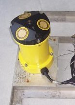
The ADCP (acoustic Doppler Current Profiler) is used to measure how fast water is moving across an entire water column. Current speeds are measured using the Doppler effect which operates through the transmission of pings of sound at a constant frequency. As sound waves travel they ricochet off particles in the water column and reflect back to the transducer which records the change in frequency of the returning soundwave. The change in frequency is called the Doppler shift and it is used to calculate how fast the particle and the water surrounding it are moving. |
This net is predominately used for surface trawls. Two different mesh sizes are used enabling collection of both zooplankton and phytoplankton samples. Zooplankton samples are collected using a 200micron net and 100 microns is used to collect phytoplankton samples. Specimens are collected into two plastic containers attached to the bottom of the nets, ready for analysis once back onboard. |
| T/S Probe | Side Scan sonar | Van Veen Grab | Digital Camera |
Niskin Bottles |
 |
 |
 |
 |
 |
| Fig 3:6 Temperature salinity (t/s) probe | Fig 3:7 Sidescan sonar on deck | Fig 3:8 Grab in a box on deck | Fig:3:9 Digital camera | Fig 3:10 Niskin bottle on rope |
|
The T/S probe contains as electrical component called a thermistor, which is sensitive to changes in the resistance of an electrical current. It is this part of the instrument which measures temperature. Salinity is a measure of the conductivity of salt particles and is carried out by two metal plates (electrodes) within the T/S probe. When an electrical current is passed between these plates within a water sample, the ease in which the current flows is an indication of conductivity. |
Sidescan sonars, commonly known as a ‘towfish’ can be used to generate large images of the sea floor known as a sidescan trace. Towed behind the research vessel at an approximate depth of 1m, a sound pulse is emitted simultaneously from two transducers either side of the towfish. When this pulse reaches the seafloor, it is then reflected and the degree of reflection is dependant on the density of the material reflecting the pulse as well as the slope of the seafloor. The sound pulse is transmitted at a frequency of 100-500 kHz indicating a long wavelength but a relatively low resolution. |
This is a metal grabbing device which can collect sediment samples from the seabed. Deployed from the back of the research vessel at designated points along the sidescan transects, the samples provide evidence of seabed composition which can support that observed on the sidescan traces. They also provide samples of benthic fauna which can be indicators of particle size, organic content and pollution. |
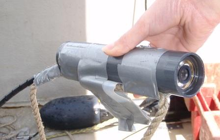
A waterproof video camera was deployed prior to the collection of sediment grab samples to observe the seabed and ensure the site was suitable to take a sediment sample i.e. the seabed was not just made up of hard rock or there was no Seagrass present which we are not permitted to grab. |
The plastic bottles are deployed through the water column using a hydroline to a pre-determined depth. They can then be closed using a messenger sent down the line from on board. The water sample is then brought back on board and can be analysed for dissolved oxygen and nutrient content. These bottles can also be attached to a CTD Rosette and closed electronically. |
![]()
 |
|
Determination of Dissolved Silicon. |
|
Determination of Phosphate. |
|
Determination of Chlorophyll. |
|
Nitrate Analysis. |
|
Oxygen analysis. |
![]()
 |
Offshore |
![]()
![]()
![]()
![]()
![]()
|
A total of three stations were fully sampled (1, 2 & 3), then a CTD drop and ADCP profile were carried out at a further 3 stations (4, 5 & 6). The first station was carried out near Black Rock to check all the equipment was working correctly. We then proceeded 45 minutes out on a bearing of 120° to station 2. We then continued a further 45 minutes on the same bearing to station 3. Time constraints and a temperature change of 1°C during sampling at station 2 and a 0.2°C temperature increase indicated by the ADCP suggested that the front may be between station 1 & 2 where the water depth decreases. Therefore station 4 was carried out approximately half way between these stations. CTD and ADCP data indicated we were not quite on the front therefore station 5 was carried out 2nm towards station 1 on a bearing of 240°. Computing errors resulted in a loss of the CTD data from station 4 therefore we returned to station 4 to repeat the CTD profile (4b). |
| Tides Mouth of the Fal Estuary: Time Type Height 0507 Low 1.4 1116 High 4.5 1727 Low 1.6 2329 High 4.6 |
Station Location |
| Raw data can be found in :\\Seahorse1\group_1\Offshore\offshore raw |
|
|
CTD & Nutrients |
 |
 |
 |
 |
 |
 |
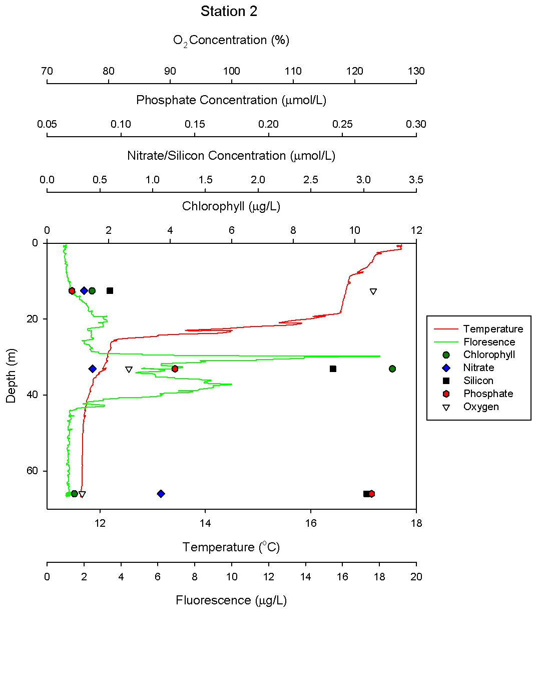
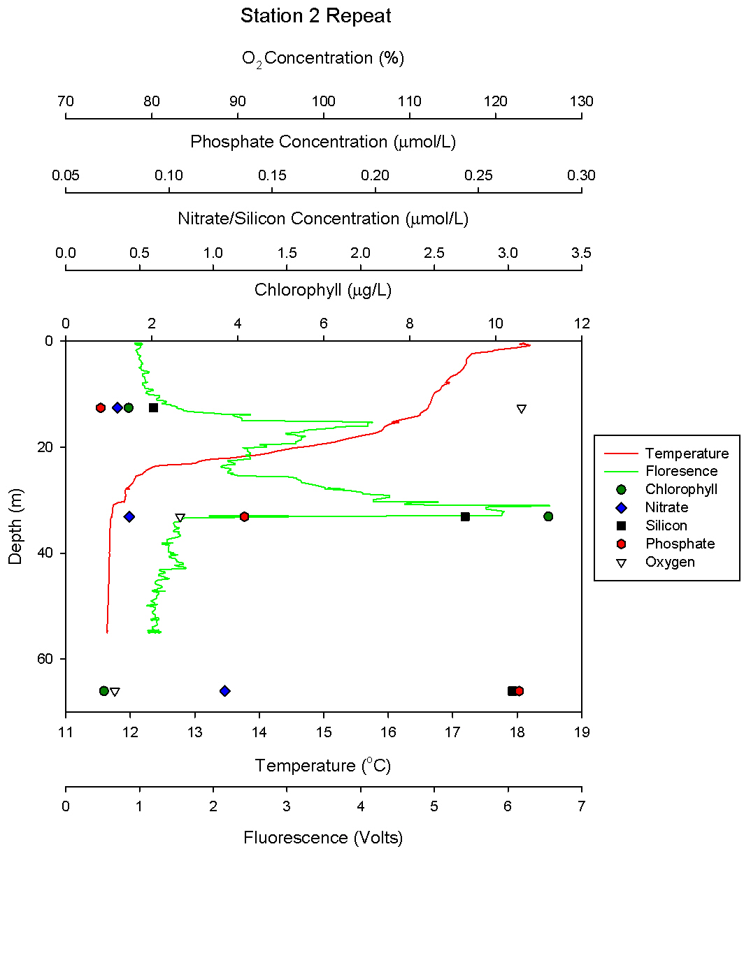
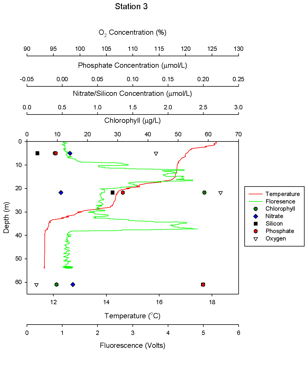
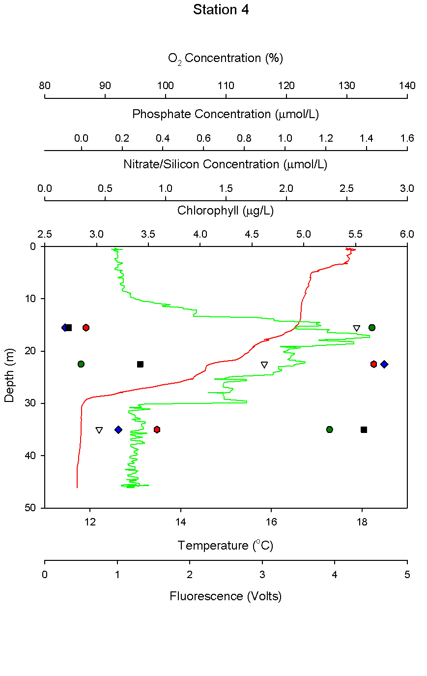
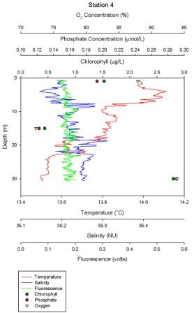
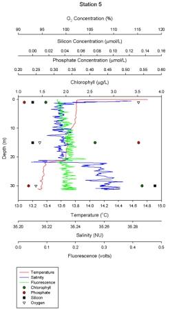
| Fig 4:1 Station 1 | Fig 4:2 Station 2 | Fig 4:3 Station 2 Rep | Fig 4:4 Station 3 | Fig 4:5 Station 4 | Fig 4:6 Station 5 |
-
|
Fig :4:7, Secchi disc depths and converted Euphotic zone depths at each of the stations. |
|
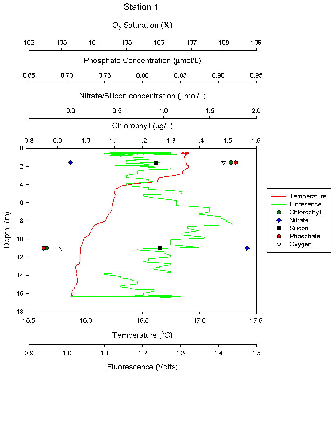
Station 1 (fig 4:1): |
|
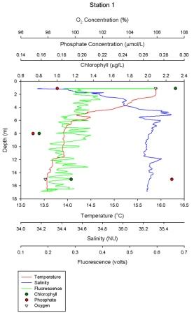
Station 2 (fig 4:2): |
|
Station 2 Repeat (fig 4:3): |
|
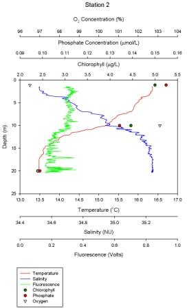
Station 3 (fig 4:4): |
|
Station 4 (fig 4:5): |
|
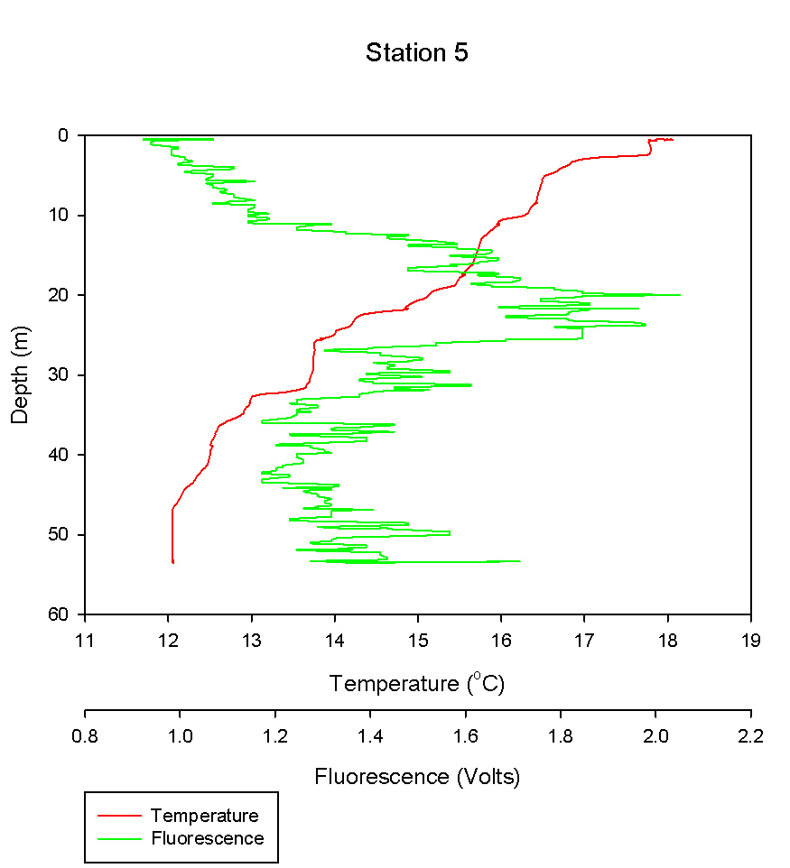
Station 5 (4:6): |
![]()
|
|
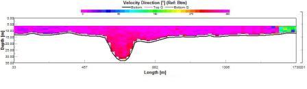
ADCP |
|
Station 1: gr1000r |
|
High levels of backscatter were recorded at the surface in the top 5m and from a depth of 6m the degree of backscatter decreased to <73dB. Station 1 is located in a channel within the mouth of the estuary therefore is bounded by regions of shallower water (<10m). Chlorophyll levels are relatively low within the surface waters with values less than 1.51µg/L (fig 4:1) however within 8-4m zooplankton number have values up to 6x10⁷ (fig 6:4). Therefore zooplankton abundance is the likely cause of high levels of backscatter and low phytoplankton abundance suggests that grazing rates are high. Although spring tides do not occur until July 7th (Featherstone & Du Port, 2009), low nitrate levels (fig 4:1) indicate that we have surveyed post a phytoplankton bloom with the mouth of the Estuary. |
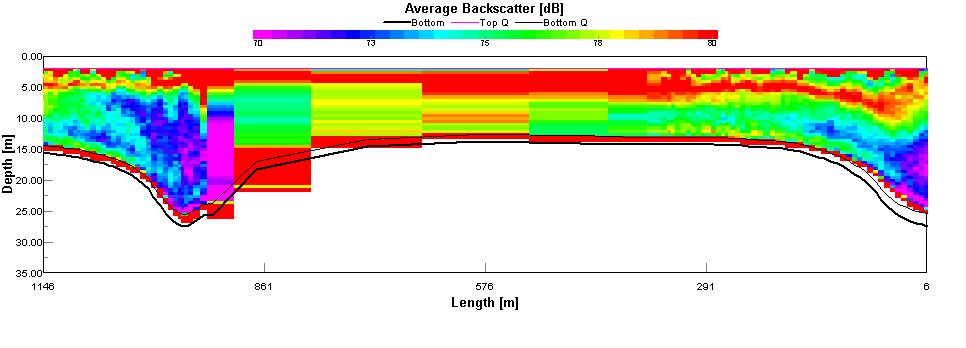 |
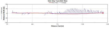
Fig:5:1 |
|
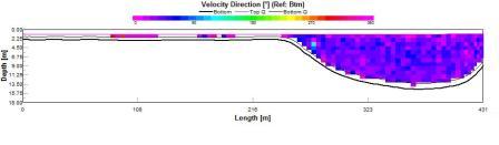
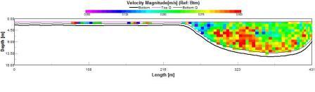
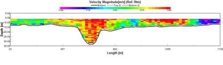
Flow velocities are relatively low at station 1 although flow is slightly enhanced at the surface with values reaching >0.25m/s. |
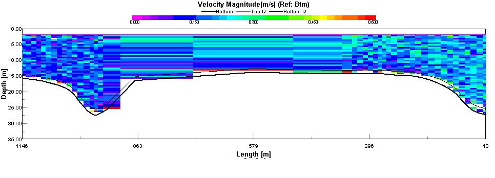 |
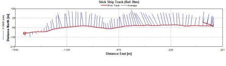
Fig:5:2 |
|
During sampling at station 1 the boat drifted therefore we repositioned ourselves before carrying out the zooplankton samples. This can be observed on the track plot. |
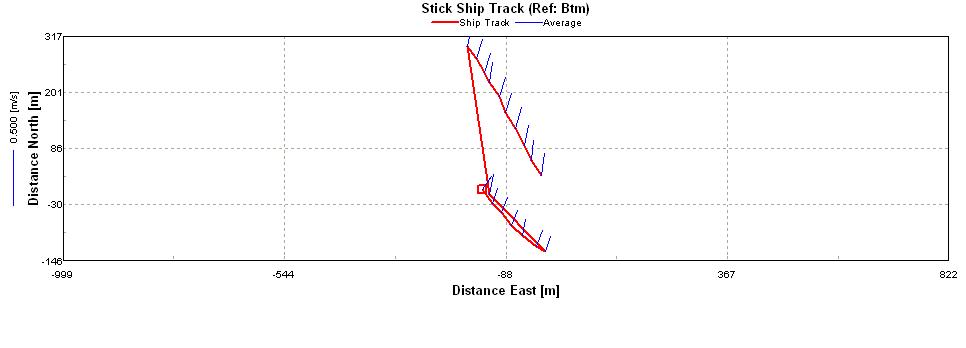 |
Fig:5:3 |
|
Station 2-gr1003r |
|
Station 2 shows two shows two distinct bands of backscatter at 23.6m and 32.11m. This shows a relatively good correlation to the CTD data taken from this station (fig 4:2) and particularly to the second CTD profile taken here (fig 4:3). Phytoplankton concentrations here were significantly greater than station 1 and predominately dominated by diatoms however zooplankton numbers were also high at the surface and down to a depth of 30m with surface values reaching 9.5x10⁷ m-3 (fig. 6:4). The high degree of backscatter is therefore likely to be caused by both diatoms which posses hard silicon skeletons (Miller, 2004) and zooplankton such as hydromedusae which were the most dominant zooplankton at 0m. |
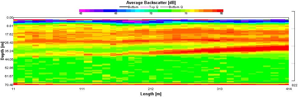 |
Fig:5:4 |
|
The velocity magnitude of flow indicates a band of high velocities up 0.37m/s from a depth of 20m to 50m. Flows at the surface and the seafloor are lower with minimum flow values of 0.1m3/s. This region of faster flow corresponds to the depth of both the chlorophyll maxima and the thermocline. |
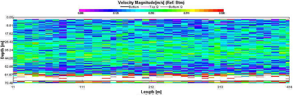 |
Fig:5:5 |
|
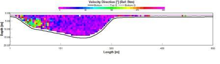
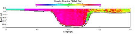
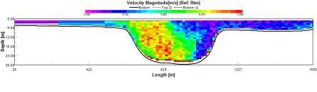
Station 3-gr1006r |
|
At station 3, the two bands of backscatter become more distinct and occur at depths of 9m and 25m. Although the fluorometer readings from the CTD data demonstrates a similar pattern (fig 4:4), the depths of the two chlorophyll maximums are slightly different with the upper maximum occurring at 15m and the lower maximum occurring at 35m. A zooplankton trawl was carried out to try to determine whether the low chlorophyll values between these two maximums were a result of grazing however zooplankton abundance from 20-20m had values of only 1.2x10⁷ m-3 (fig. 6.4). This is the second lowest zooplankton abundance value from all four stations. Chlorophyll concentrations from the discrete water sample taken at 21.75m, just below the first chlorophyll maximum record by the fluorometer indicates phytoplankton abundance is still high therefore an error may have occurred with the fluorometer during sampling. |
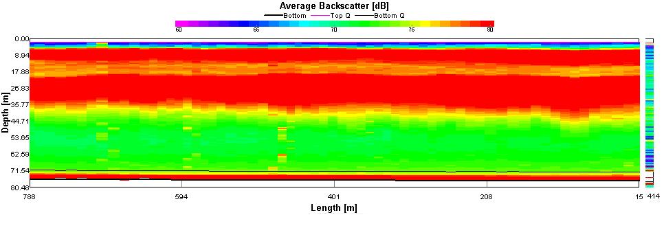 |
Fig:5:6 |
|
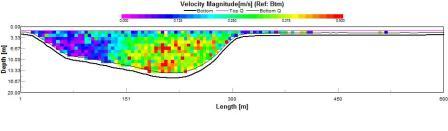
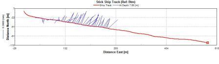
During station 3, the velocity magnitudes appeared to change considerably with relatively high values of 0.3m/s at the beginning throughout the entire water column. The average velocities then decreased to 0.27m3/s. Surface values to a depth of 7.6m are consistently low however, at the seabed velocities of flow reach 0.96m3/s. |
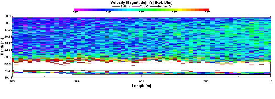 |
Fig:5:7 |
|
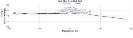
Station 4-gr1008r |
|
There is a very strong band of backscatter from 30-35m which is slightly deeper than the chlorophyll maxima observed on the CTD profile. However the discrete water samples taken at a 34m depth showed consistently high chlorophyll values of 5.3µg/L (fig.4:4). Additionally, the phytoplankton counts taken at 35m recorded the highest total abundances of all the samples taken with concentrations of 21204 per 100ml (fig. 6:3). The dominant phytoplankton at this depth were dinoflagellates however, high abundance here are surprising as the depth of the euphotic zone calculated using the secchi disk was only 23.1m. This indicates that mixing must be occurring pushing phytoplankton below the euphotic zone. Unfortunately no zooplankton samples were taken at station 4. |
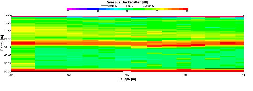 |
Fig:5:8 |
|
In contrast to station 2 where velocities where higher mid water column, the velocities at station 4 appear to be highest at the surface and seafloor with velocity values of up to 0.32m3/s. In contrast the lowest velocity values were recorded at a depth of 33m with a value of 0.03m/s. This data does not support above explanation of high phytoplankton concentrations below the euphotic zone and weak thermocline. |
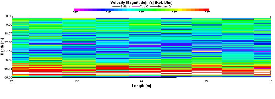 |
Fig:5:9 |
 |
 |
 |
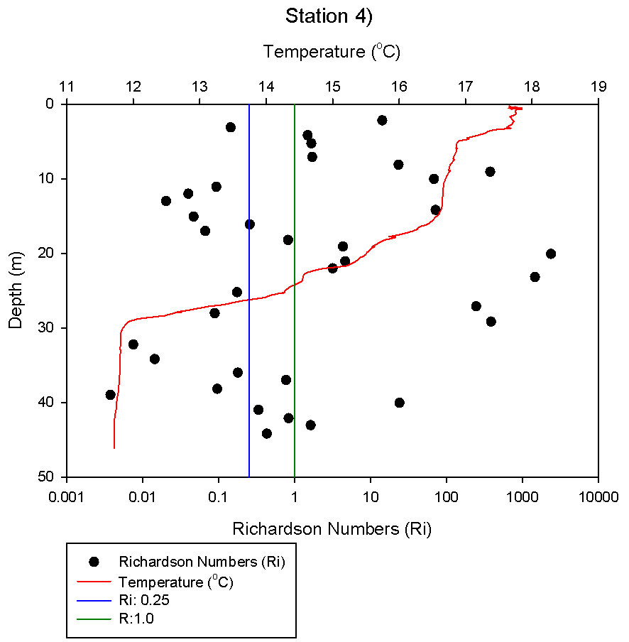 |
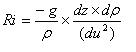
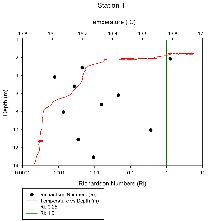
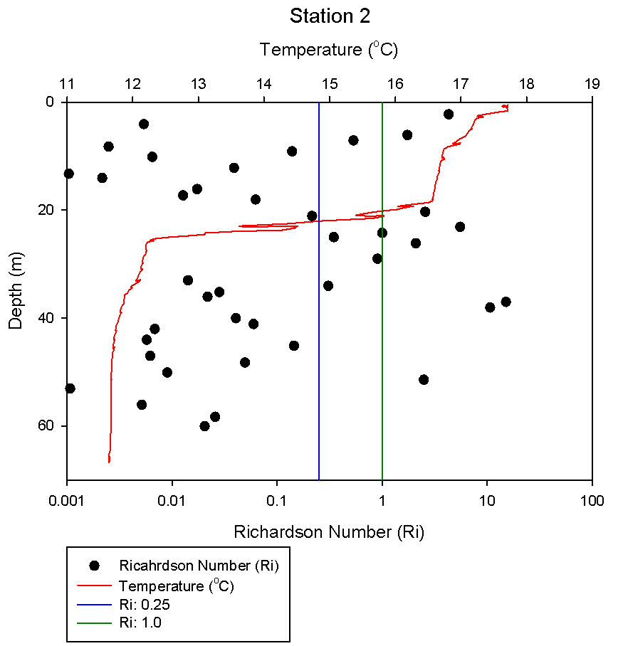
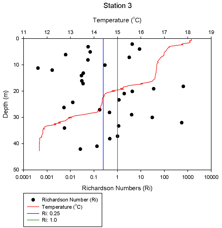
| Fig:5:10 A graph displaying the Richardson number and temperature with depth at station 1 | Fig:5:11 A graph displaying the Richardson number and temperature with depth at station 2 | Fig:5:12 A graph displaying the Richardson number and temperature with depth at station 3 | Fig:5:13 A graph displaying the Richardson number and temperature with depth at station 4 |
|
The Richardson number is a measure of the flow stability of a body of water. It is calculated by comparing the densities and velocities of different ‘sections’ within the water column, using the following equation:
At all stations, the Richardson numbers were calculated every half metre throughout the depth of the water column. With the exception of a few anomalies, the Richardson numbers (Ri) along the thermoclines were greater than 0.25 indicating that there is little or no mixing occurring and stratification within these regions is strong. Ri values below 0.25 are indicators of mixing and occur in regions where the temperature profile is vertical or near vertical and the temperature is uniform with depth. This pattern is complicated at station 3 where there are internal processes occurring creating a double thermocline. Additionally at station 4 (fig 4:5) within a well mixed region down to a depth of 15m, the Richardson numbers indicate that there is both areas of stability and instability. Whilst it was initially thought to be caused by very low velocity values, analysis of the ADCP data indicates that this was not the case. Sampling at station 4 was carried out at 1439 (GMT), three hours before high water therefore flooding waters of speeds up to 0.4m/s were observed at the station. In conclusion a more precise comparison of ADCP data and Richardson values is required for a more comprehensive analysis of vertical stability profiles. |
![]()
|
|
Plankton |
| Phytoplankton Abundance at each of the sample stations |
 |
 |
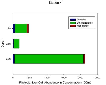 |
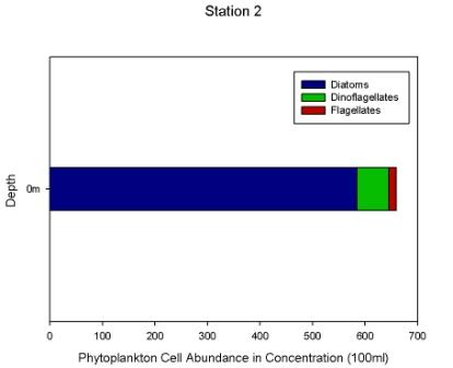
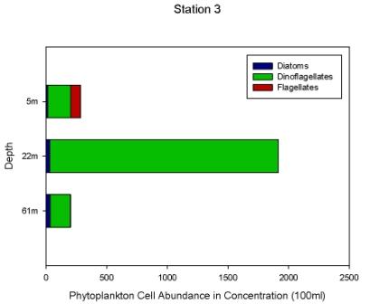
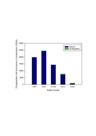
| Fig 6:1 Bar chart of Phytoplankton abundance taken from Station 2 | Figure 6:2 Bar chart of Phytoplankton abundance taken from Station 3 | Fig: 6:3 Bar chart of Phytoplankton abundance taken from Station 3 |
|
Samples for phytoplankton were collected at stations 2, 3 and 4. Station 2 was a surface trawl sample and at stations 3 and 4 various depths were sampled. The cell count of diatoms may appear smaller than the actual amount in the water column, as only chains of diatoms were counted rather than individual cells. Diatoms dominated surface waters at station 3. Out of the 5850 diatom cell counted in the sample, 4700 were Chaetoceros. Both dinoflagellates and flagellates were also recorded in smaller numbers. At station 3, dinoflagellates dominated, the most abundant species being Karenia mikimotoi. Karenia mikimotoi is usually found in calm stratified waters and are relatively small in size so do not easily sink through the water column. Two thermoclines, recorded at around 20m and 30m indicate highly stratified waters. There were also two chlorophyll maximums recorded for this station at depths of 15m and 40m, with a significant depletion at around 20m. Diatom numbers increased slightly with depth, with highest numbers recorded at 61m. As diatoms are fairly heavy they do fall out of the water column, particularly in stratified waters. Although higher numbers of diatoms were found at 61m, species diversity at 22m was highest with 7 genus groups counted. Station 4 was dominated by dinoflagellates, highest numbers were recorded at a depth of 35m, this abundance is predominately Karenia mikimotoi. Although diatoms often dominate coastal waters, dinoflagellates will become more predominant with distance from land (Pinet 2006). Flagellates were present in shallow depths and again at depth, but none were recorded at 22m. At this depth there was an overall lack of phytoplankton compared to other stations and depths with only 1850 cells counted. Generally Karenia mikimotoi was the most abundant phytoplankton group at each depth for stations 3 and 4. |
|
Zooplankton |
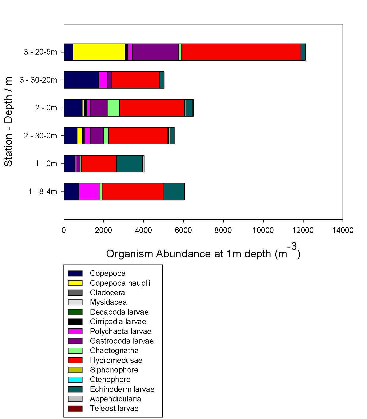 |
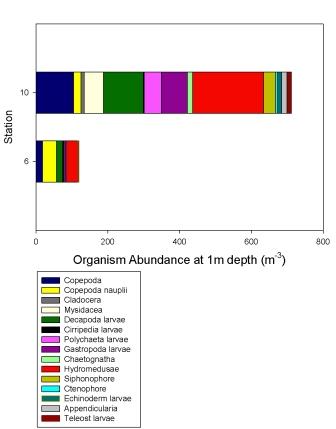
| Fig 6:4 Bar chart of the Zooplankton abundance at each of the sample stations |
|
Zooplankton samples were collected from stations 1, 2 and 3. Samples were collected using niskin bottles deployed at various depths. From figure 6:4 it is evident that the organism abundance is highest in the samples collected from the surface. The maximum total zooplankton abundance was observed at the surface at station 2, this showed a value of 9.5x10⁷ m-3. At each station zooplankton abundance reduces with depth, the lowest total zooplankton abundance was found at station 1 from the 8-4m sample at a value of 6.8x10⁶ m-3. Hydromedusae are the most abundant group at each depth, at each station, with greatest abundance at the surface at station 2 of 4.78x10⁷ m-3. Copepoda and copepod nauplii grouped together make up the second largest section in samples from stations 2 and 3. In the 0m sample from station 1 Echinoderms were recorded as the second largest zooplankton group. The surface waters from station 2 also showed Echinoderm to be prevalent. The high levels of zooplankton were found in surface waters as this is where food resources such as plankton and other zooplankton are most abundant. However this is not reflective of the phytoplankton data which shows relatively low abundance at 0m for station 2 and 5m for station 3. The data shows that the water column is dominated by hydromedusae. This may be put down to patchiness as a result of zooplankton behaviour such as vertical migration and swarming. A wide range of stirring and mixing methods can interact with biological processes to produce plankton patchiness (Abraham, 1997). However, the high numbers of hydromedusae witnessed may be a reflection of the seasonal variation. All hydromedusae larvae are released at the same time of year, it is likely that this is what is being observed. |
![]()
|
|
Discussion |
|
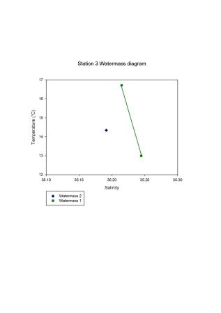
Prior to surveying on 29/06/2009, the SW coast of England had been experiencing anticyclonic conditions (http://www.metcheck.com/V40/UK/FREE/synoptic.asp). Low wind speeds and high temperatures associated with these weather conditions can result in reduced mixing leading to a shallowing of the mixed layer as stratification within the water column increases and the seasonal thermocline decreases in depth. This was particularly observed at station 1 where a slight thermocline was recorded at a depth of 2-4m (fig 4:1). With a euphotic depth of 27m and a water column depth of 18m, phytoplankton should be able to photosynthesise within the full depth of the water column however chlorophyll levels were relatively low throughout. Nutrient concentrations, particularly nitrogen were very low within the surface waters indicating that primary production at the mouth of the estuary was nutrient limited. Further offshore, the thermocline became more pronounced and at station 2 had increased from 4m to 20m (fig 4:2). The temperature profile at station 2 indicates very stratified surface waters and by station 3, a double thermocline has developed. A TS diagram was constructed to determine whether this physical feature was a result of mixing of two different water masses however, Figure 7:1 concluded that this was not the cause of the observed temperature ‘step’. An alternative explanation could be that alternating regions of stratification and mixing within the water column could force a temperature profile like that observed in figure 4:4. Group 9 who carried out the same survey also observed an unusual temperature profile at station 3 which could represent the onset of a double thermocline. Our data was recorded during very warm, calm weather when small internal density differences were the dominant mixing process. Group 9 however, carried out the exact same station 4 days after a storm event when wind mixing had completely overturned the water column and the temperature profile was only just re-establishing itself. There could be a number of reasons for such an unusual temperature profile and would a very interesting topic to investigate further. Station 3 also had a very interesting double peak in the fluorescence data indicating two bands of phytoplankton. This would be most easily explained by a band of zooplankton between the two phytoplankton peaks where grazing had reduced the number of phytoplankton however, our data shows that the zooplankton levels at this depth are very low (fig 6:4). If the temperature profile is in fact a result of two water masses coming together this double peak could be a result of one water mass containing high numbers of phytoplankton and the other containing low levels. Station 4 was carried out in between station 1 & 3 to attempt to identify the location of the front. We were unsuccessful in this aim as we would have expected to see an outcrop of the thermocline at the surface yet the surface waters were still relatively well mixed down to a depth of 5m. We did nevertheless observe a very good transition profile from station 1 to station 2. |
|
![]()
 |
Geophysics |
![]()
![]()
![]()
![]()
|
Weather: Fine, Sunny, 6 Oktas |
Tides:
(GMT) Low Tide: 01:47 4.326m |
| Raw data can be found in: \\Seahorse1\group_1\Geophysics\SSrawData |
|
|
|
Transect 1 |
Transect 2 |
|
Transect 3 |
Transect 4 |
|
|
 |
 |
 |
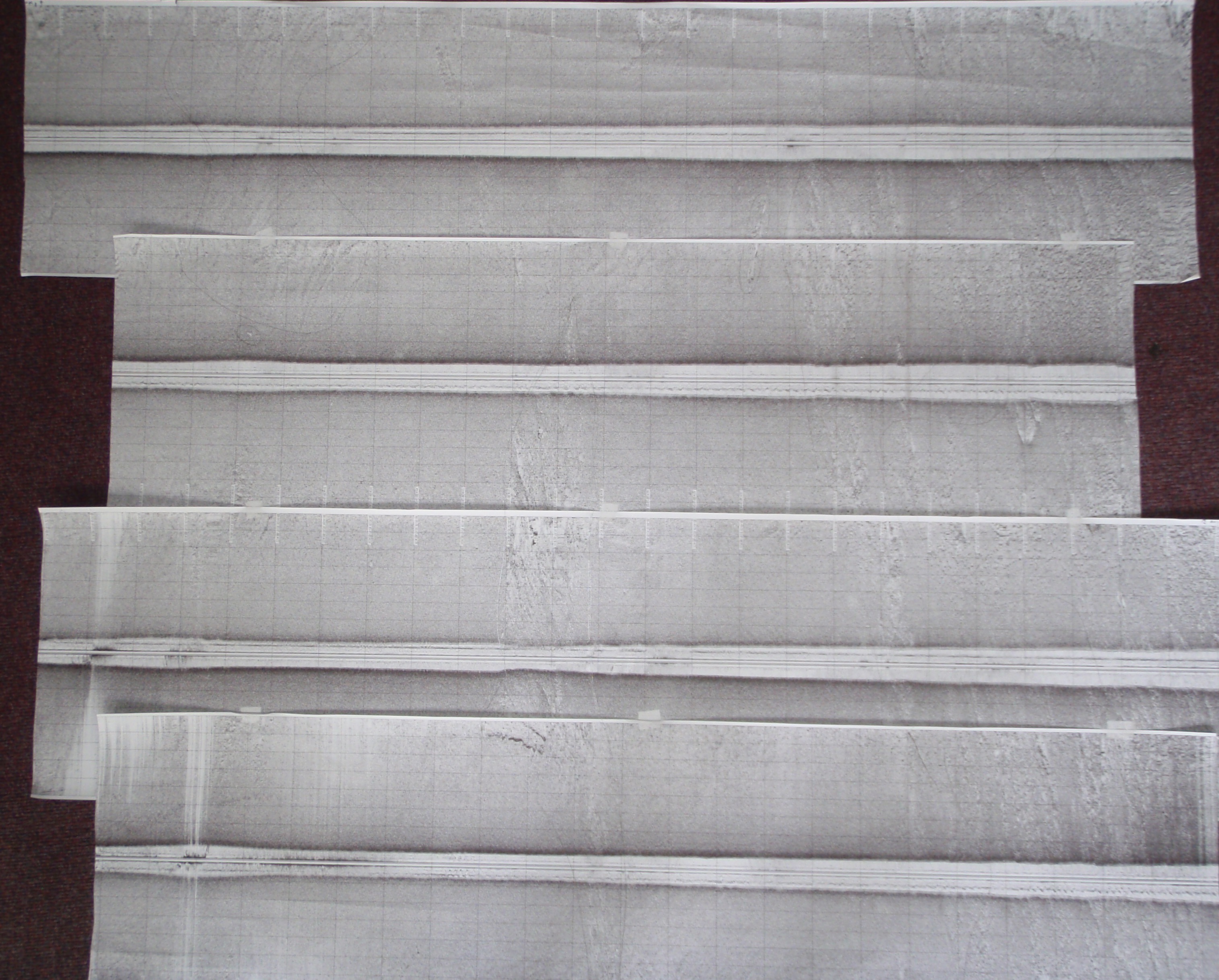
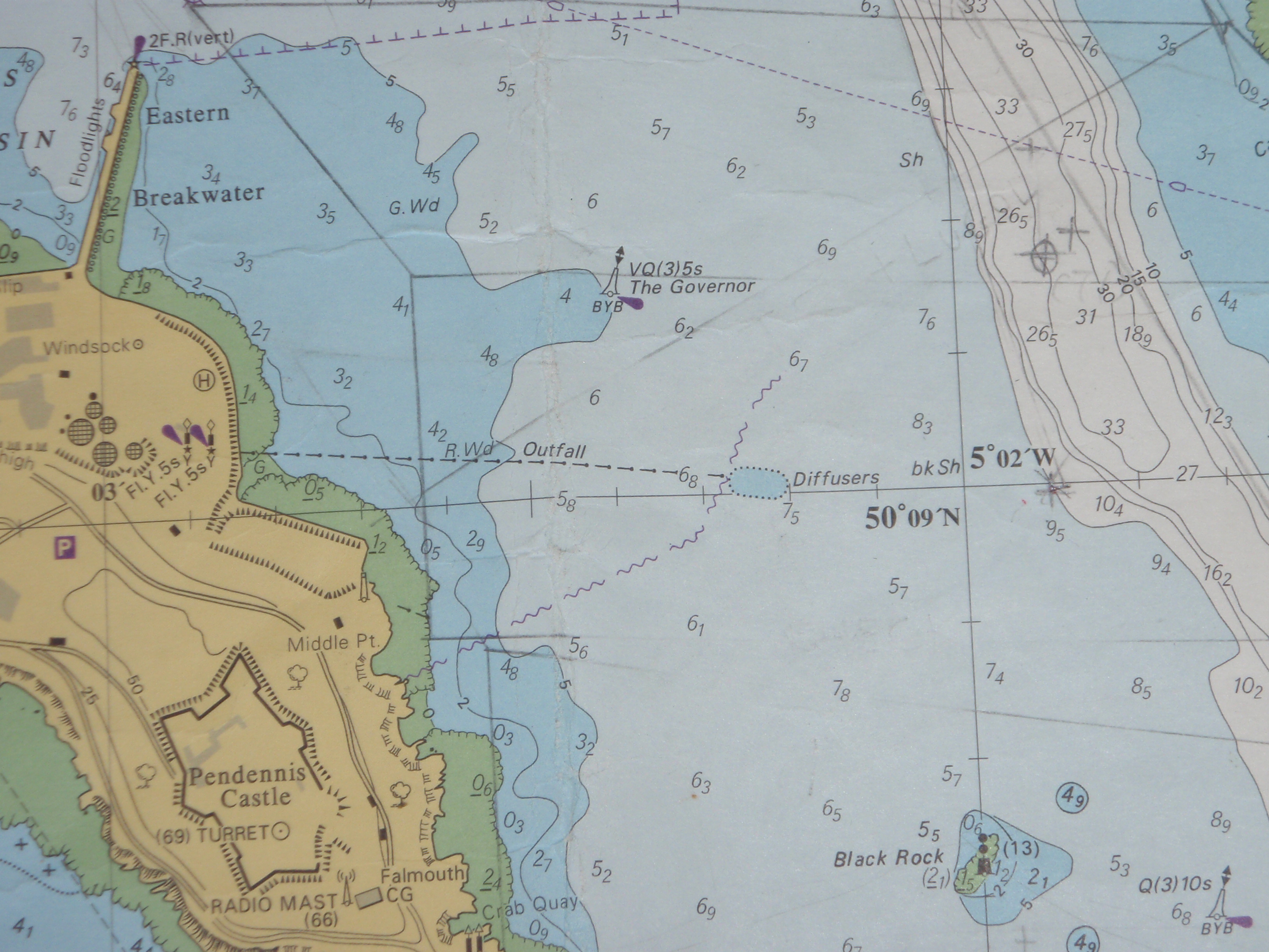
| Fig: 8:1 Image of the transects taken on the Fal estuary | Fig: 8:2 Thermograph print out of the sidescan sonar taken from fig:6:1 | Fig: 8:3 close up of chart on the diffuser out let into the Fal estuary | Fig 8:4 Thermograph of diffuser out let into the Fal estuary |
![]()
|
|
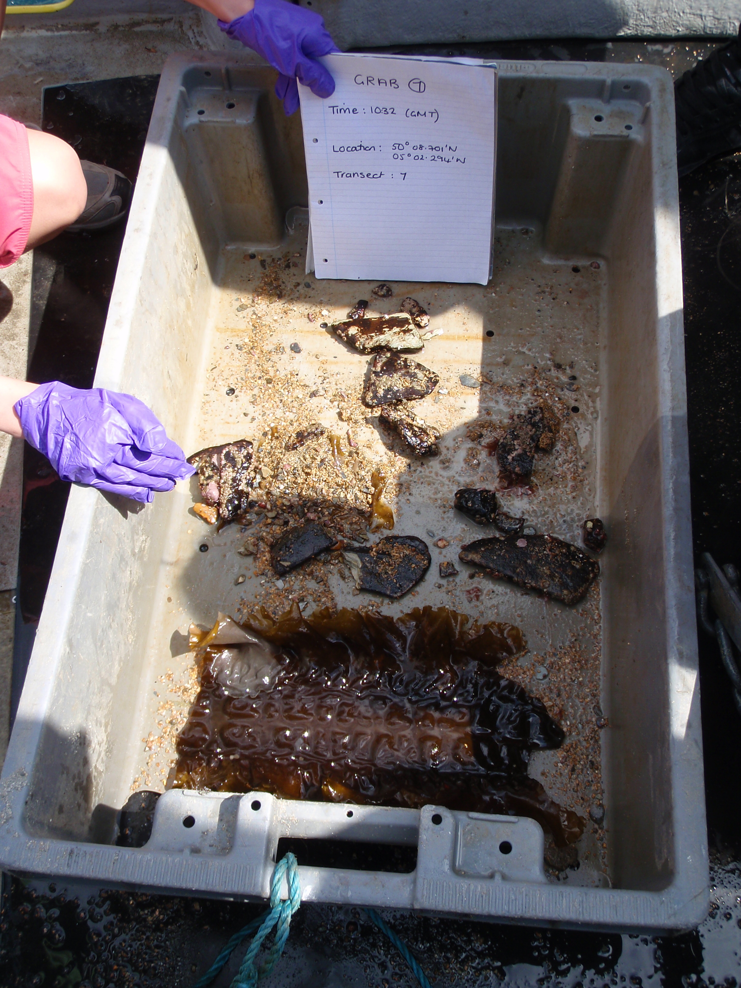
GRAB 1
Transect:
1 Sediment: Poorly sorted. Predominately gravel (2-4mm) & shell fragments with some large stones (64-256mm) (Wentworth, 1922). Benthic Fauna:
|
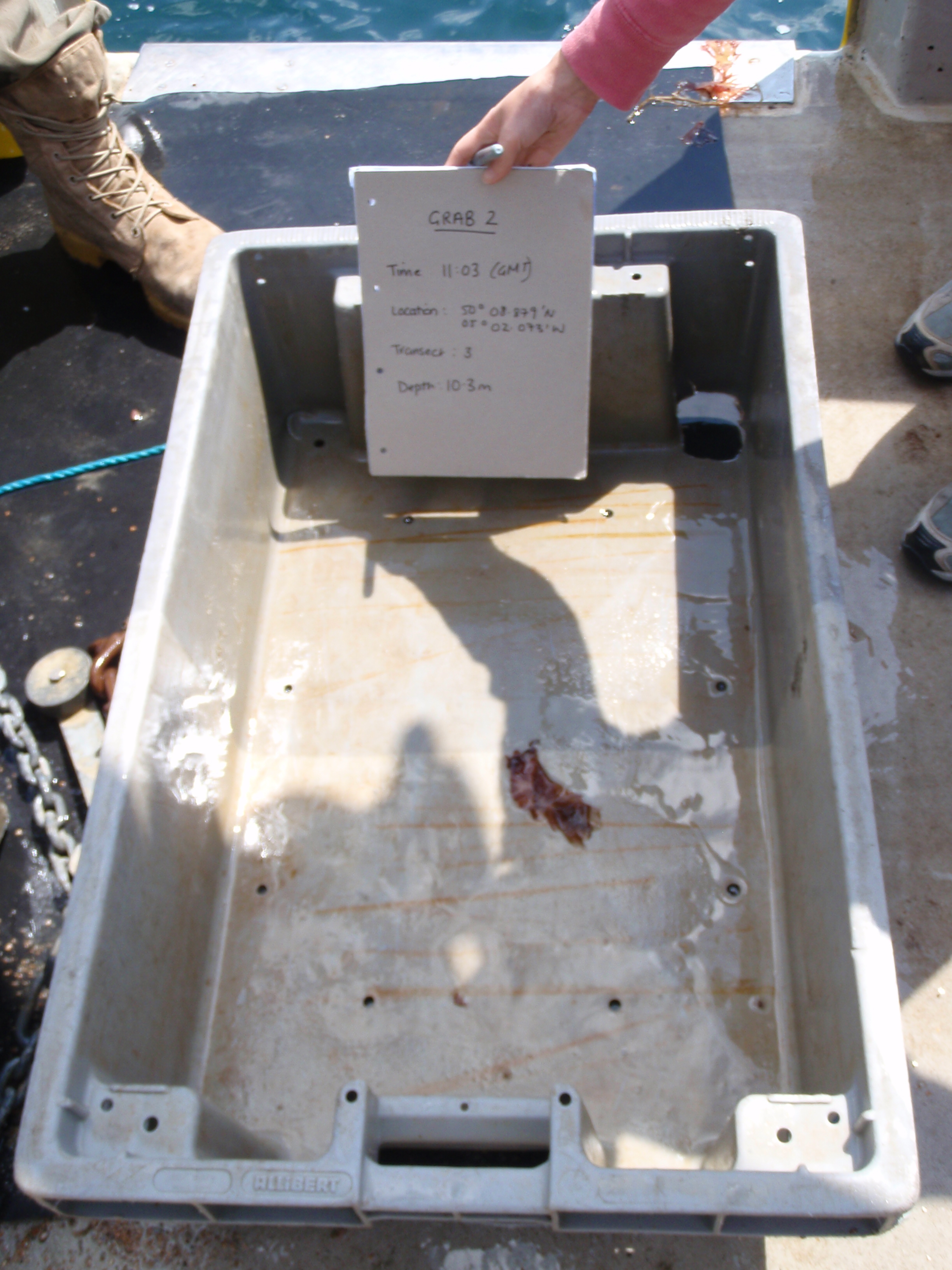
GRAB 2
Transect:
3 Sediment: No sediment collected in grab indicating a hard rocky substratum. Benthic Fauna:
|
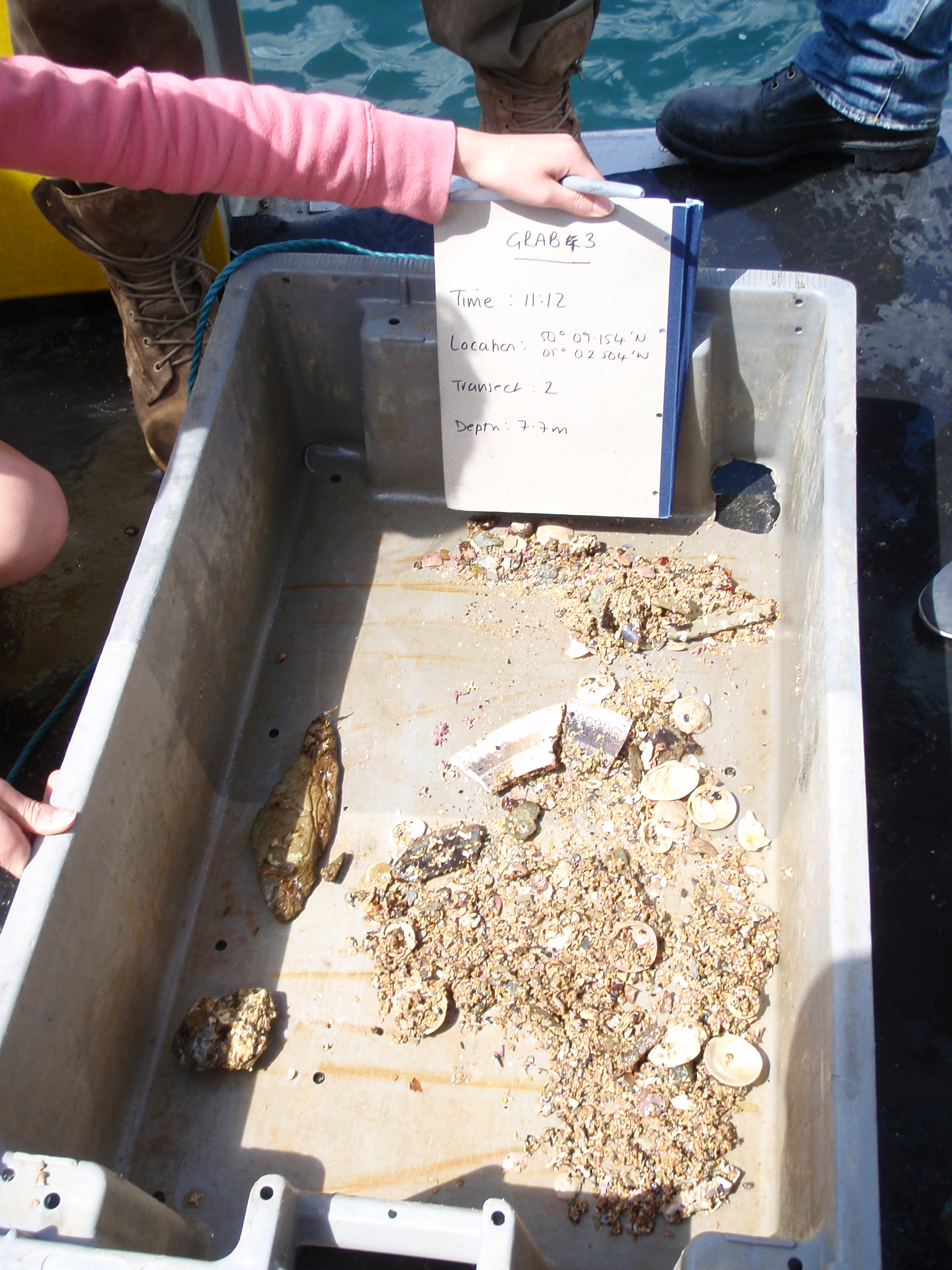
GRAB 3a
Transect:
2 Sediment: Poorly sorted. Predominately small gravel particles and shell fragments. Benthic Fauna:
|
|
 |
 |
 |
|
||||||||||
|
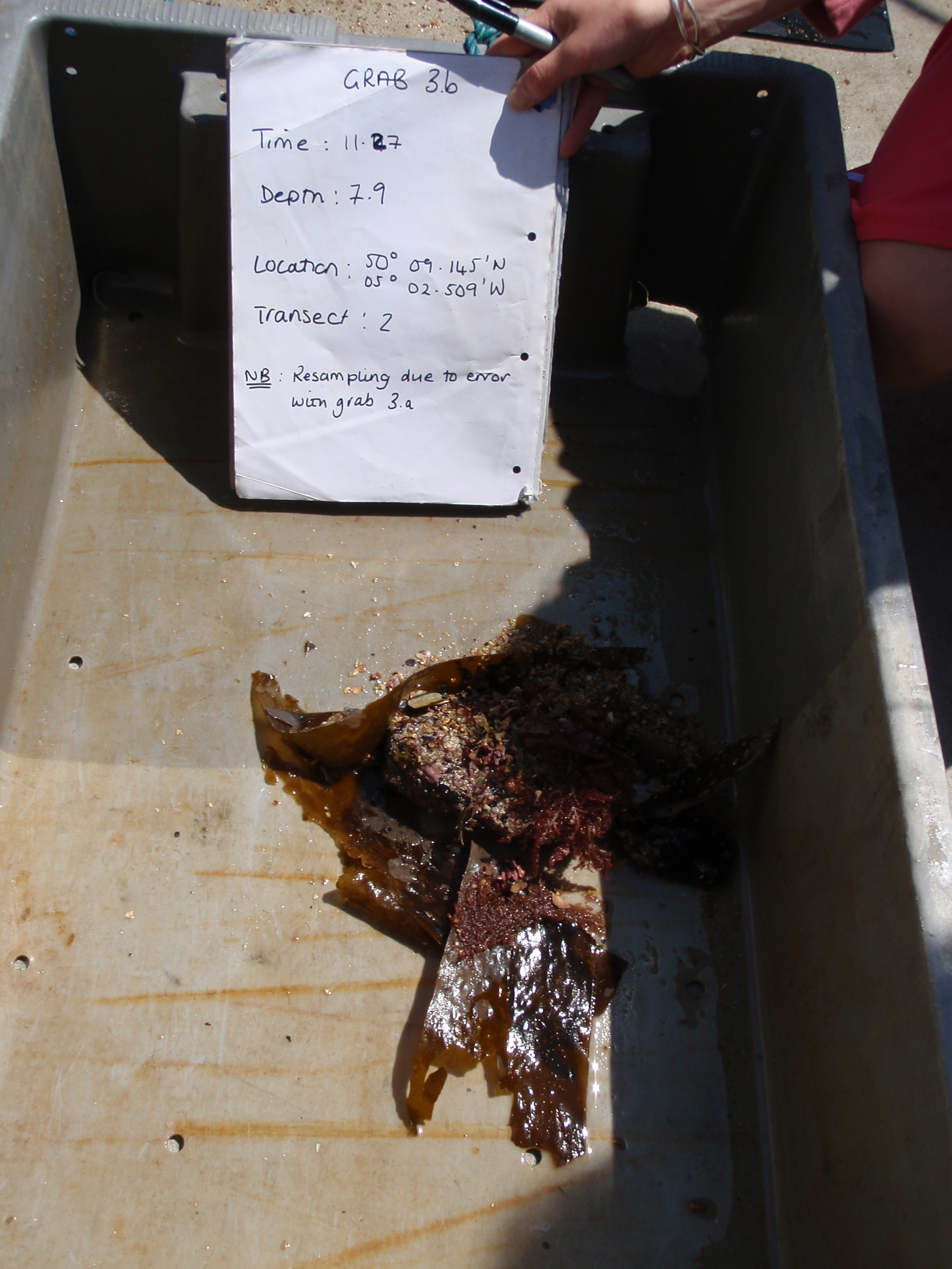
GRAB 3b Transect: 2 Time: 1127 Location: 50˚09.145’N, 005˚ 02.509’W Depth: 8.0m A large stone got caught within the mouth of the grab so a large amount of sediment was lost during retrieval of grab 3a therefore a second grab (grab 3b) was taken. Sediment: Poorly Sorted. Predominately gravel with some shell fragments and medium grained sands (0.125-0.5mm) (Wentworth, 1922). Benthic Fauna:
|
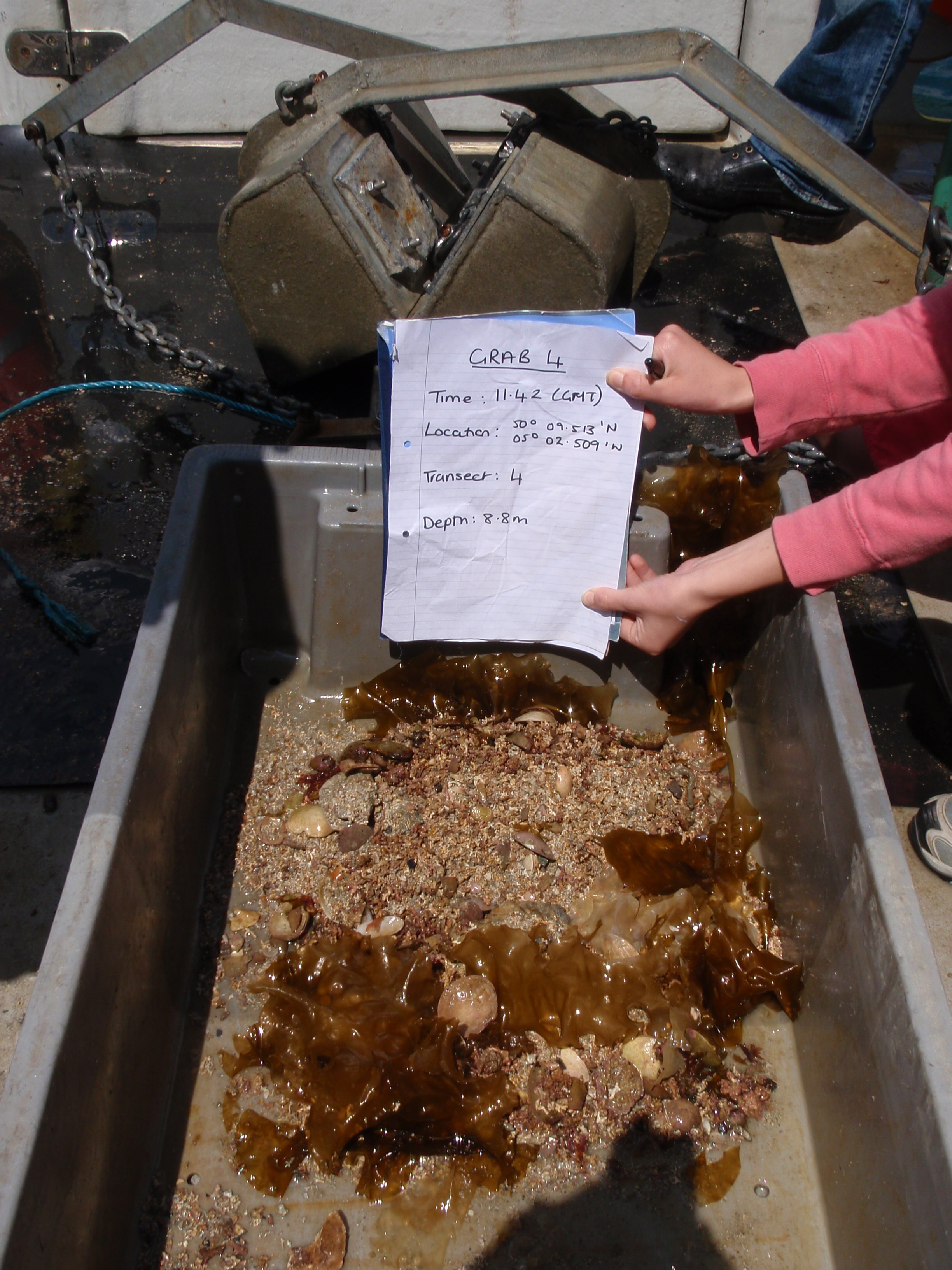
GRAB 4 Transect: 4 Time: 1142 GMT Location: 50˚ 09.523’N, 005˚ 02. 475’W Depth: 9.1m Sediment: Mainly comprised of Maerl with some fine grained sand particles (0.125-0.5mm) and shell fragments. Benthic Fauna:
|
|||||||||
 |
 |
|||||||||
| Fig 8:8 Photo of Grab sample 3b | Fig 8:9 Photo of grab sample 4 |
![]()
|
|
Discussion |
| The area surveyed was close to the coastline with several large patches of rock. This substrate provides attachment sites for dense kelp forests which were also observed at a number of sites along the transects (fig 8:1). From the maritime chart it was determined that a marine outfall and diffusers were traversed. The diffusers were observed on the sidescan projection although the outfall was not (fig 8:4). The maritime chart shows that the substrate of the area is predominately broken shell and gravel. The unmarked area on the track plot is assumed to be made up of this material. The area marked as possible kelp is difficult to interpret. It is possible that there is some suspended particulate matter (SPM) due to noise in the water column. This area could be representative of sand waves, variances in turbulence. There is not enough supporting evidence to draw sound conclusions as to what has caused these observations. |
![]()
 |
![]()
![]()
![]()
![]()
![]()
|
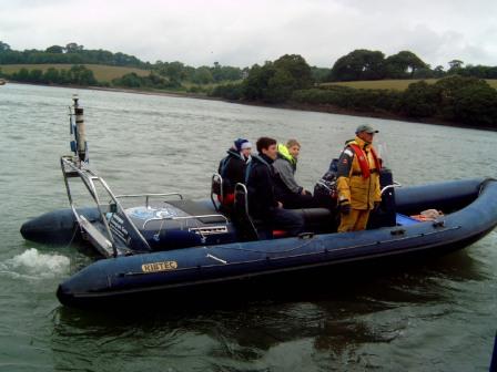
The upper and lower parts of the Fal Estuary were sampled to investigate the longitudinal and vertical variations of temperature, salinity, oxygen, turbidity, nutrient and plankton. The aim was to observe the chemical, physical and biological variations that occur with the estuary as a result of its structure and the mixing processes that occur. The residence time of the estuary will also be calculated. Samples from the upper part of the estuary will be collected via a rib where water samples will be collected to measure nutrients and plankton abundance. Temperature, salinity, oxygen and pH will be recorded using a YSI probe. Samples from the lower part of the estuary will be collected onboard the research vessel R.V. Xplorer. A CTD rosette will be used to measure the same parameters and water samples will also be collected from three different depths at the five stations to determine phytoplankton abundance and nutrient concentrations. Zooplankton net trawls will also be carried out at each station. A time series will also be carried out at a pontoon during the morning which is located just south of King Harry Ferry on the river Fal at latitude 50°12.980N and longitude 5°01.659W. Here YSI recording will be taken every half hour and water samples every hour. Finally, five ADCP transects will be carried out longitudinally across the estuary in the afternoon onboard R.V. Xplorer. The first transect will be taken at the head of estuary and the final one at the mouth. Between these locations an additional 3 transects will be carried out in order to observe changes in the physical structure and flow rates within the estuary. |
|
Tides
Time Type Height (m) 0415 High 4.6 1101 Low 1.4 1632 High 4.9 2325 Low 1.4 |
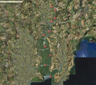 |
Fig:7:1 Map of thr Fal estuary |
| Fig: 9:1 Upper Fal estuary survey stations on the RIB | ||||||||||||||||||||||||||||||
|
| Fig: 9:2 Lower Fal estuary survey stations on Explorer | ||||||||||||||||||||||||||||||
|
| Fig: 9:3 Pontoon survey site | ||||||||||||||||||||||||||||||||||||
|
| Fig: 9:4 ADCP survey transects across the Fal estuary | ||||||||||||||||||||||||||||||||||||||||||
|
| Raw data can be found in: \\Seahorse1\group_1\Estuary\Raw Data |
|
|
 |
 |
 |
 |
 |
| Fig: 10:1 Station 1 | Fig: 10:2 Station 2 | Fig: 10:3 Station 3 | Fig: 10.4 Station 4 | Fig: 10.5 Station 5 |
|
Station 1 (fig:
10:1)
|
|
Station 2 (fig:
10:2) |
|
Station 3 (fig:
10:3) |
|
Station 4 (fig:
10.4) |
|
Station 5 (fig:
10:5) |
|
|
|
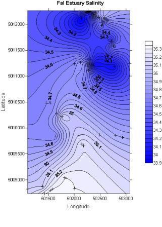
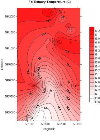
| Fig: 10:6 A contour plot of surface salinity readings across the Fal estuary. | Fig: 10:7 A contour plot of surface temperature reading across the Fal estuary. |
|
The TS contour plots indicate that the highest temperatures are observed within the upper reaches of the estuary were water depth is low. The deep central channel within the estuary can therefore be observed on temperature contour. Conversely, salinity values are lowest in the upper reaches and according to the salinity contour plot, there appears to be two regions of high salinity. It is important to note that the resolution of the TS probe is only 0.1. On closer examination, these regions occur where a large number of samples were taken during the CTD station however, there looks to be a plume of fresh water coming down the estuary. Although the data was collected during a flooding tide, sampling was carried out extremely close to the entrance of Truro River therefore there maybe a surface flow of freshwater although this can not be identified within the ADCP data for transect 1. |
|
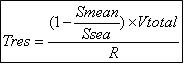
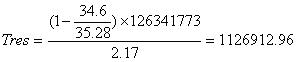
Residence Times:
Where:
= 13.04 days |
Tidal Flushing:
Where:
= 17.7 hours |
|
Tidal Prism:
Where: Vprism= 24,820,000 x 3.5 = 86870000m2 |
|
Assumptions & Considerations:
These calculations are based on a number of assumptions and are therefore only rough indications of residence and flushing times. This is evident from the disparity between the two values and therefore can only be considered as approximate values for the Fal estuary. The residence time calculated using river flow rates is expected to be a larger value than that calculated using the tidal prism method because the Fal estuary is predominately a tidal dominated estuary. |
![]()
|
|
ADCP |
|
Transect 1 & 2 Transects 1 & 2 were both carried out at the bottom of the Truro River which feeds into the Fal estuarine basin however transect 1 included the output from Pill creek. The maximum depth along this transect was 13.61m and the flow throughout the water column was unidirectional in a northwestly direction. This is indicative of a flooding tide and therefore water flow along transect 2 was also in a NW direction. Along transect 1 however there is a slight reversal of flow along the western boundary of the estuary where riverine inputs with a maximum flow of 0.031m/s from Pill Creek are disrupting the flow. The highest velocity recorded along transect 1 was 0.513m/s whereas the maximum flow along transect 2 was only 0.493m/s. The highest velocities were observed in the deeper regions and decreased towards the shallower areas at the edges of the estuary. Transects 1 was carried out on slight bend in the channel therefore higher velocities were observed on the outside of the bend. It is important to note that the ADCP transect carried out at station 1 was recorded the wrong way round and proceeds right to left instead of left to right (West to East). |
|
|
Transect 3 Transect 3 was also completed during the incoming tide however the maximum velocity along this transect was greater than transect 1 & 2 with a value of 0.568m/s. An ebbing flow was also observed along the western side of the estuary due to the riverine inputs from the Carnon River which flows through Restronguet Creek. Flows speeds here were found to be approximately 0.187m/s. Additionally the velocity maximum occurred within the water column at a depth of 13.61m and surface velocities were around 0.286m/s. |
|
|
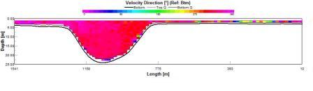
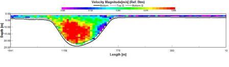
Transect 4 The ADCP data shows that along transect 4, the main tidal flow is within the deep channel with a maximum of 4.94m/s. This region of high velocity, unlike transect 3, extends from the surface down to the seabed and although velocities were greatest at a depth of approximately 19.6m, the velocities at the surface were still comparatively high with values of 0.492m/s. Either side of the deep central channel there are shallower regions with an average depth of 5.6m and along the western boundary of the estuary a reversal of flow is observed and at a depth of 5.6m reached a velocity of 0.254m/s. |
|
|
Transect 5 The data for transect 5 was collected the following day (08/07/09) by another group because the ADCP data file collected on the 07/07/09 became corrupted during transect 5. This repeat transect was carried out at 1425 (GMT), during a flooding tide therefore a similar profile was expected. The ADCP profile showed two distinct regions were velocities were higher. The first was within the deep estuarine channel; surface velocity values here reach 0.566m/s. A second region was found just north of Black Rock with velocities of 0.6m/s. This region which lies to the west of the main estuarine channel could be a result of eddying within the estuary and the presence of black rock at the mouth of the estuary could enhance this. Additionally high riverine inputs of fresh water from Percuil River could also result in instabilities and mixing at the mouth of the estuary. Although velocities decrease towards the edge of the estuary where the water depth decreases, higher velocities were still observed along the western margin of the estuary. Flow direction also reversed below a depth of 6.60m with water flowing out of the estuary at the margin. Again this could be a result of lagging tides or the influence of Black Rock. |
|
![]()
|
|
Plankton |
 |
| Fig: 12.1Phytoplankton abundance through out the estuary across 5 stations |
|
Bottle samples 67, 81 and 104 were taken from the upper end of the Falmouth Estuary within the River Truro. Bottle samples 21 and 23 were taken from the lower and of the Falmouth Estuary with salinities decreasing respectively. Generally diatoms are the dominant phytoplankton group within the sampled area, dinoflagellates are present at all sampling points but often numbers were significantly smaller. Bottle sample 67 was taken from the lowest salinity point; here diatom cells dominate the phytoplankton population within the surface water. Cell count for diatoms was recorded at 19818 calls per 100ml, compared to only 10 cells per 100ml for dinoflagellates. Sample 81 was taken from a stationary pontoon downstream of the first sampling point. Diatom cell numbers increased from the previous station to 24228 cells per 100ml, dinoflagellate numbers also increased to 263 cells per 100ml. This is the maximum cell count for diatoms, subsequently cell count decreased with rising salinity values from this sampling point. This maximum could be linked to the high values of silica recorded within this area, as silica is utilised in the production of frustules in diatoms. Dinoflagellate numbers increased slightly at sampling point 21; here values reached a maximum of 657 cells per 100ml. This could be explained due to changes is phytoplankton dominance. Diatoms can inhabit different environmental niches (for example different salinities, lower light levels, different levels of nutrients) and it is possible that unfavourable conditions have lead to diatom decrease, enabling other phytoplankton groups to dominate, in this case dinoflagellates. Significantly lower values of diatoms were found in sample 23 where cell counts were recorded at 554 cells per 100ml. The major phytoplankton groups found were Chaetoceros, a form of diatom chain, and Alexandrium and Karenia, both dinoflagellates. |
 |
| Fig:12.2 Zooplankton abundance across 2 stations with the Fal estuary |
|
Zooplankton samples were collected aboard the R.V. Xplorer by trawling a 200 µm plankton net at approximately 2 knots for 5 minutes . The samples were obtained from the top of the water column at station 6 and station 10. Station 6 is the furthest north station from the Xplorer, where the estuary narrows into the River Fal, station 10 is at the mouth of the estuary (fig 12.2). Figure 12.2 shows that at the mouth of the estuary the total number of zooplankton nearly 6 times greater than that at the head of the estuary. The proportion of each group of zooplankton at each station is similar however there are notable differences. The four largest groups of zooplankton are the same at each station, these are Hydromedusae, Decapoda larvae, Copepoda and Copepoda nauplii. Although at station 6 Copepoda and Copepoda nauplii together make the largest group totalling 57 organisms m-3, whereas at station 10 the largest group is hydromedusae at 197 organisms m-3. Another difference is the much smaller proportion of Gastropoda larvae and Polychaeta larvae at station 6 than at station 10. The structure of the zooplankton community at station 10 resembles that of the zooplankton sample collected from offshore (fig 6:4). The high proportion of hydromedusae at station 10 is therefore also considered to be a combination of patchiness and seasonal variation. The zooplankton community of station 1 (mouth of the estuary) from the offshore data shows large proportion of Echinoderm larvae, however at station 10 from the estuary data the Echinoderm larvae proportion is much smaller. This difference is likely to be identification error. |
![]()
|
|
Discussion |
|
Physical structure of the Fal Estuary: The high salinities recorded at station 1 on the rib and the relatively low residence time calculated indicates that the Fal estuary is a predominately saline estuary where the effects of tidal flows are the major controlling factor of physical structure within the estuary. The reversal of flow observed along the entire western boundary of estuary implies that small scale internal instabilities are occurring which can result from interactions with the sea floor. No layered flow was observed with depth indicating a uniform flow. This would suggest that the Fal is a well mixed estuary and homogeneous salinity profiles were indeed observed at station 4 & 5. Further up the estuary figure 10.1 indicates that a layer of saltier water is flowing over a layer of well mixed water. This could be a result of the strong flooding tide and it is likely that if we were to sample at the same locations on the subsequent ebbing tide, we would see a more homogenous salinity profile further up the estuary. The temperature profiles from the CTD stations indicate that from station 3 to station 5 which is located at the entrance of the estuary, thermal stratification is occurring within the water column. Salinities here are relatively homogenous irrespective of tidal state, therefore temperature variations are the most important factor leading to density instabilities and thermal mixing becomes the most dominant mixing process. This situation is reversed in the upper reaches of the estuary were large salinity variations, which have a greater effect on density per salinity unit compared to a 1oC temperature change. Turbidity at all stations remained very similar (between 4.15 and 4.5 volts on the transmissometer) however, the profiles show a decrease in turbidity down the estuary, possibly due to the loss of particulate matter from the water column as the river water is slowed down on contact with seawater. This also results in an increase in the depth of the euphotic zone. The offshore stations displayed a greater variation in turbidity at and between the stations, but there was a general trend towards slightly higher turbidities than recorded in the estuaries. Peaks in the turbidity were found at depths equating to the thermocline of each station, which is consistent with the large number of phytoplankton found at these depths. At station one, the turbidity is low and the euphotic zone extends to the seabed. The depth of the euphotic zone decreases as the stations move further offshore. Chemical: The nitrate estuarine mixing diagram provides a textbook example of non-conservative behaviour where removal from the water column at the mouth of the estuary has resulted in a decrease in concentrations below the TDL. The estuarine mixing diagrams for silicate and phosphate however portray a more complicated picture where there appears to be non-conservative behaviour yet an injection of both nutrients at salinities of 27. This salinity value was observed on the rib at station 1, right at the very head of the (fig.10:1) and lower salinity values were only recorded in the samples taken from streams further inland. Due to very low concentrations within the lower part of the estuary, the estuarine mixing diagrams represent a distorted view of the estuary because no samples were taken between salinities 4.5 and 27 yet there is some sort of large input of nutrients between these two stations and beyond this point phosphate and silicate appear to act conservatively. However silicon concentrations are completely depleted in the lower part of the estuary. Whilst this input could be from runoff due to the large rainfall that has occurred in the last two weeks, elevated values would have also been observed in the lower part of the estuary. It is unlikely that high silicon concentrations are a result of a large diatom mortality event because the abundance of diatoms throughout the estuary was very high with abundances reaching a maximum at station 2 where salinities were 30.2. Our data is therefore inconclusive. Biological: The phytoplankton abundance within the estuarine system was considerably different to that observed offshore. Diatoms dominated from the head down to the mouth of the estuary however Dinoflagellate abundance did increase from station 4. Station 1 offshore was carried out in almost the same location as Station 4 of the estuary however the phytoplankton sample taken here was lost therefore we were unable to make a comparison at this station. Diatom abundance was still high at station 2 which is an indication that diatoms may also have been the most abundant phytoplankton at station 1. This is surprising because silicon concentrations where not depleted on 30/06/09 and diatoms were abundant but by the 07/07/09 silicon concentrations near Black Rock were completely depleted yet diatoms remained abundant. It would be interesting to investigate the silicon concentrations measured offshore on 07/07/09 see if a there was a comparative decrease in silicon offshore. At station 3 & 4 offshore, dinoflagellates remain the dominant which is indicative of the calm, stratified conditions observed. The zooplankton abundance was considerably greater offshore than within the estuary however the community structure within both systems were relatively similar. Hydromedusae remains the most dominant group however numbers become considerable reduced at station 6, the furthest most estuarine sample. Here copepod nauplius is the most dominant however this group is one of the most dominant at station 3 offshore. One notable difference is the increase in larvae, particularly Decapod larvae within the estuary where water depth is lower and shoreline habitats create ideal nursery grounds. |
![]()
| References |
|
Abraham, E.R. (1997). The generation of plankton patchiness by turbulent stirring. Nature 391: 577-580. Cornwall Holidays, (1996) [image] Available at http://www.chycor.co.uk/falmouth.htm [accessed 7 July 2009] (fig 1:2) Digital Globe, (2009) Google Earth [online] Available athttp://www.earth.google.com (fig1:1) Featherstone. N., Du Port. A. (2009). Reeds Nautical Almanac, UK Pinet P.R, (2006) Invitation to oceanography. Jones & Bartlett Publishers inc Grasshoff, Kremling K, Ehrhardt M. (1999) Methods of Seawater Analysis 3rd Edition. (Wiley-VCH) Johnson, K. S. and R. L. Petty. (1983) Determination of nitrate and nitrite in seawater by flow injection analysis. Limnology and Oceanography, 28, 1260-1266 Langmuir, I. (1938). Surface motion of water induced by wind. Science 87:119-123. Miller, C.B. (2004). Biological Oceanography. Blackwell Publishing Ltd. Parr.W, Mainstone. C, P. (2002) Phosphorus in rivers- ecology and management. The Science of the Total Environment pp282 283 Vol 25 47 Parsons, T.R. Maita, Y. And Lalli, C. (1984) ‘A manual of chemical and biological methods for seawater analysis’ 173 p. Pergamon. Joint Nature Conservation Committee, (1999). Special Areas of Conservation- Fal and Helford [online] updated 2006. Available at http://www.jncc.gov.uk/protectedsites/sacselection/sac.asp?EUCode=UK0013112). [Accessed 8 July 2009]. Langston et al., 2003- mining within the fal estuary catchment. Just google & it should come up. Metcheck, (1999). Atlantic Synoptic Charts [online] updated 6 July 2009. Available at http://www.metcheck.com/V40/UK/FREE/synoptic.asp- [Accessed 6 July 2009]. Neville, J., Womack, J. University of Washington, (2006). Quartermaster Harbor [online]. Updated 2006. Available at http://courses.washington.edu/uwtoce06/webg2/methods/methods.html. [Accessed 6 July 2009]. South East Atlantic Coastal Ocean Observing System, (2003). Current Measurement Technology [online] updated September 2008. Avaliable at http://seacoos.org/Data%20Access%20and%20Mapping/current_tech. [Accessed 8 July 2009]. Environemental Agency, (2001). River flow rates for the UK [Online]. Updated 2006. Available at http://www.nwl.ac.uk/ih/nrfa/webdata/048003/g2001.hmtl [Acessed 7 July 2009]. |
![]()
|
The Views and Opinions expressed are those of the individuals and not those of the university |