Falmouth Field Course 2008

Group 9

Jordan Salmon   Gavin Morrison   Jenny Caston   Ed Mendelsohn   Steff Deane

Tasha Stone   Zoë Sterland   Jenny Adams   Briony Silburn   Ray Bell

1. Introduction

Introduction

The Fal Estuary is situated in Cornwall, South West England. It is a drowned river valley, or ria, with a maximum depth of 33m. This makes it the third deepest natural harbour in the world. There are six main tributaries entering the estuary, as seen in Figure 1.1, but despite this freshwater input rates are low. The main section of the estuary is known as Carrick Roads and is characterised by a deep central channel. Either side of this the estuary floor is broad and shallow, ranging from 0.3-4.6m in depth. The local geology dates back to the Devonian period, with meta sedimentary rocks dominating, such as carnmellis granite, metamorphic aureole and china clay.

                                                                    

The Fal Estuary is macrotidal during a spring tide, with a maximum range of 5.3m and mesotidal during a neap tide, with a range of 3.5m. Based on the Hansen-Rattray diagram, the estuary can be classified as a well-mixed estuary during a spring tide, or partially mixed during a neap tide.

                                                                               

Prevailing winds from the South West and shelter by the local morphology, creates a warm and windy climate. Average sea surface temperatures range from 9ºC in the winter to 16ºC in summer. The average salinity of offshore waters is 35 and the average maximum tidal current speed is below 2 knots.

The presence of extensive Maerl beds has earned the Fal Estuary the status Site of Special Scientific Interest. However, extraction of these rare calcareous species, by dredging, still occurs today. Other anthropogenic effects include oil pollution, anti-fouling releases and sewage, with industrial effluents causing significant detriment to the biology of the estuary. Increased nutrient levels from sewage can cause harmfull algal  blooms of the toxic dinoflagellate Alexandrium sp., These bloom events are commonly known as a red tide.

Mining has been a dominant anthropogenic feature in the Falmouth area since the Bronze Age with the last tin mine, Wheal Jane, closing in 1992. However, the effects of acidic drainage are still evident from flooding and erosion of old mines causing Restronguet Creek to be the  most heavily metal polluted estuary in the UK. Additionally, Copper concentrations in the Fal Estuary currently exceed the European Quality Standard level of 5µml^-1. Consequently many species in the estuary have developed a tolerance to these high metal concentrations,  especially to copper.

We aim to assess the biological, chemical, physical and geophysical aspects of the Fal Estuary and its immediate offshore region.

2. Vessels

RV CALLISTA

This research vessel was used for offshore sampling. Its size allows for simultaneous multiple equipment deployment and sample analysis. Facilities include wet and dry labs, onboard computers and an upstairs seating area useful for team working.

              Specification                                              Deck

RV BILL CONWAY

The RV Bill Conway was used for the upper estuarine studies. Its relatively large stern  allows for the deployment of multiple pieces of equipment simultaneously.

              Specification                                              Deck

OCEAN ADVENTURE RIB

The RIB's small size and good maneuverability is well suited for sampling the upper estuarine and riverine environments. The shallow draft allows the RIB to obtain data in areas where the RV Bill Conway is restricted.

            Specification                                            

SV XPLORER

The survey vessel Xplorer is used for geophysical studies. Equipment including Side Scan Sonar and Van Veen grabs are used to obtain bathymetric data.

            Specification                                              Deck

3. Equipment

CTD AND ROSETTE

A CTD continuously records conductivity (salinity), temperature and depth providing detailed information about the water column, distinguishing features of scientific interest and therefore indicating the important depths at which to sample. The CTD is mounted on a metal frame, or rosette, which enables other sampling equipment to be attached, such as Niskin bottles and a fluorometer.

NISKIN BOTTLES

These plastic bottles are attached to the rosette and come in a variety of volumes. There are 6 bottles attached at any one time collecting water samples throughout the water column from pre-determined depths. The bottles use a trigger mechanism consisting of shot messengers which are released from onboard the research vessel and sent down a wire to the bottle. The samples can then be used for chemical and biological analysis.

Acoustic Doppler Current Profiler

The ADCP measures the speed and direction of currents in the water column. Pulses from multidirectional transducers are reflected from the seabed or particles within the water column and recorded. This signal is digitally processed to produce a visual interpretation of the current. The Doppler shift causes the return pulses to vary with frequency and from this direction and speed of the currents is deduced. Repeating this process produces a time series data set.

Transmissometer

The transmissometer measures turbidity within the water column using beams of light. A receiver detects the backscatter light levels, thus indicating the amount of light absorbed or scattered by particles in the water column.

Side Scan Sonar

Side Scan Sonar is used to survey the topography and sediment type of the sea floor. It is mounted on a tow fish and is towed behind the vessel. Transducers emits pulses of ultrasonic waves and the reflection from the sea floor is recorded. A black and white image is produced which can be used to interpret sediment type and bathymetric features, which in turn can indicate current intensity and direction. The Side Scan Sonar may be used a two frequencies of which the higher produces an image of narrower swath but higher resolution.

Secchi DisK

The Secchi disk gives an estimation of the Euphotic depth. It is lowered into the water and the Secchi Depth (depth when it can no longer be seen) is recorded. The 1% light level or the Euphotic depth is three times the Secchi disk depth.

Plankton Nets

Zooplankton nets (mesh size 200µm), are used to collect plankton samples and can be towed both horizontally and vertically. A flow meter is attached to the net  to give tow speed and the tow area can be determined by net diameter and tow time.

Flourometer

A fluorometer measures chlorophyll concentration within the water column, exciting the phytoplankton by emitting light at a set wavelength. This causes them to emit light at a different wavelength which is measured by the fluorometer.

Van Veen Grab

The Van Veen grab collects benthic sedimentary samples from the sea bed. On contact  with the sea floor the grab automatically closes. The sampled sediment can then be analysed on board the vessel or later in the lab.

The anemometer is a hand-held piece of equipment used to measure wind speed. It can be measure in both m/s and km/hr.

YSI Probe

The YSI probe is a multi-parameter probe used on board the smaller vessels. It measures  temperature, salinity, chlorophyll, turbidity, pH, dissolved oxygen levels and depth.

A temperature and salinity probe is a hand held probe to measure the temperature and salinity of the water column. Salinity is measured indirectly by determining the conductivity of the water. The TS Probe is ideal for use on small vessels.

4. Lab Analysis

Water samples collected were analysed using methods listed below:

NITRATE ANALYSIS

Nitrate concentrations were calculated by flow injection analysis (Johnson and Petty, 1983). The standards used were 1, 5, 10 and 25 µM.

PHOSPHATE ANALYSIS

A mixed reagent was added to the sample and absorbance values were determined using a Hitachi U-1800 Spectrometer (Strickland and Parsons, 1972). The standards used to calibrate the sample were 0 (blank), 0.07, 0.15, 0.30, 0.75, 1.5 and 3 µmolLˉ¹. The cell size used in the spectrometer was 4cm.

SILICATE ANALYSIS

A mixed reagent was added to the sample to change its colour depending on the concentration of silicate present. The absorbance was then calculated using a Hitachi U-1800 Spectrometer (Strickland and Parsons, 1972). The standards used to calibrate the sample were 0 (blank), 1.4, 2.8, 7.1, 14.2, 21.4 and 28.5 µmolLˉ¹. The cell size used in the spectrometer was 4cm.

DISSOLVED OXYGEN ANALYSIS

The samples were analysed for dissolved oxygen using the Winkler method (Grasshoff et al., 1999). The amount of thiosulphate (ml) added to the sample was recorded, as well as the glass bottle weight. These were then inputted into a pre-prepared equation to calculate oxygen saturation percentage. 

CHLOROPHYLL ANALYSIS

The filter papers were left refrigerated over night in test tubes of 90% acetone. The samples were then analysed using a 10-AU Fluorometer to give a fluorescence value which was used to calculate the chlorophyll concentrations (Parsons et al., 1984).

PHYTOPLANKTON TAXONOMY ANALYSIS

The samples were left to settle over night. The surface of the liquid was removed, leaving 10ml of the concentrated phytoplankton sample. This was de-cantered in to a phile and 1ml was transferred to a Sedgewick Rafter. The sample was analysed under the microscope, counting and identifying the number of phytoplankton present in 20 squares.

ZOOPLANKTON TAXONOMY ANALYSIS

When sampled, 10% formalin was added to 500ml of sample to preserve the zooplankton. In the lab the sample was well mixed before de-cantering 30ml into a sub-sample container. Using a pipette, 5ml of the sub-sample was transferred to a Bogerov tray and analysed under the microscope. The zooplankton present were counted and identified.

5. Offshore

METHOD

On 07/07/08 a survey from Black Rock to an area 15 nautical miles south west was taken.

6 ADCP transects were taken at a 2kt cruising speed to create horizontal profiles. At 8 stations between transects vertical profiles were taken.

Click here to see a map of all the transects.

Click here to see a map of all the station positions.

Below is a summary of Station position and time of sampling:

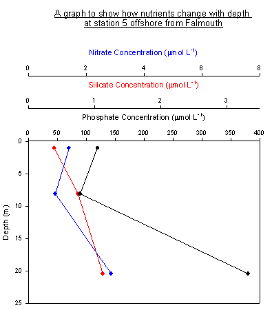
At each station, the following tasks were carried out:

RESULTS

RV CALLISTA CTD ANALYSIS

Click on the Station names to view the CTD graphs.

Click here to see a map of all the CTD stations.

Light decreases exponentially with depth at all stations. Generally at the surface the upwelled light is at -0.1, decreasing to values of -0.4 at 40m, for example at Station 8. Turbidity is typically 0.5 to 1 NTU, and in general varies little with depth. However, at Station 4 turbidity increased significantly between 20-30m to approximately 2NTU. Additionally, at Stations 6 and Station 8 the turbidity increased to 1.7NTU beyond 30m depth. At Station 8 there was an extremely high peak in turbidity at 30m, where values were elevated to 2.7NTU. This coincides with the depth of the thermocline and therefore an increase in chlorophyll, i.e. plankton. Also at Station 8 the high abundance of zooplankton may have affected the backscatter pulse which calculates turbidity.

The temperature plot shows that the thermocline decreases in depth the further offshore. For example, at Station 1 located near Black Rock, the thermocline is at 5m, where as at Station 8, located 14 nautical miles offshore the thermocline is situated at approximately 30m depth. Most stations exhibit a sharp decrease in temperature at the thermocline, with an exception of Station 5, where the change was more gradual. Salinity is opposite to temperature, in that it increases with depth. However, it follows the same pattern as temperature, in that the sharp change is located at the thermocline. The surface values for salinity vary little, typically from 35.1 near shore, to 35.2 offshore. The further offshore the higher the maximum salinity at depth, reaching 35.31 at Station 8.

Chlorophyll, which is related to the abundance of plankton, is highest above the thermocline, with a sudden decrease below. This is possibly due to zooplankton and phytoplankton species being trapped in the surface layer. At Station 4, Station 5 and Station 8 the chlorophyll maxima is directly above the thermocline. Usually the chlorophyll maxima is expected to be at the thermocline, but due to the weather conditions - low irradiance and strong winds - mixing is increased and thermal heating decreased. As a result the thermocline has been significantly reduced (compared to previous years data) and the surface layer more mixed.

RV CALLISTA ADCP analysis

Click on the transect names to view the ADCP graphs.

The ADCP is the key instrument to help indentify the initial presence of a front offshore. Due to the stormy conditions in the previous day and little solar irradiation causing stratification the front is likely to be well mixed and not clear. It will therefore be useful to look at the backscatter and velocity magnitude for each transect to compare.

The tide was ebbing at 0904 GMT after low tide at 0827 GMT during Transect 1 across Black Rock. The ADCP velocity magnitude shows a high surface velocity. The tidal flow is moving out and has an added influence on the surface from the fresh riverine water. The backscatter shows a place of high surface backscatter up to 99dB, 284m along the plot. This was created by the wake of a passing battleship and must be ignored.

Transect 2 shows that backscatter becomes steady at ~10m, 76dB. There is some concentration of zooplankton and sediment, which are the main particles which reflect the wavelength of the ADCP, at this depth showing the presence of a thermocline. Backscatter is high at the surface and bottom. This is caused by high levels of shearing from wind and sediment, respectively. This is constant throughout all the images.

Transect 3 shows an area of low backscatter 1400m along the track with a value of 65-70dB around 26m. This is due to the depth of the water column becoming greater than 45m. Bottom turbulence will not reach this high in the water column and therefore cause the backscatter to remain low.

Transect 5 shows high backscatter at ~22m deep in the water column. The back scatter is at 77dB, where as the areas directly above and below are approximately 70dB. A strong thermocline can be observed as the material assembles at this depth in the water column. Phytoplankton can be found in high numbers at the thermocline as they do not sink to the layer below and nutrients are high from mixing beneath. Zooplankton then feed on the phytoplankton and are recorded by as backscatter due to the wavelength emitted by the ADCP.

Transect 6, 13 milles offshore shows the affect of wind against current. On the day of sampling the winds were comeing from the west and the current moving south-westerly. The surface water above 20m had an average velocity of 0.4m/s where as below 20m the velocity is approximately 0.6m/s. The backscatter shows two lines of high results, one at 12m depth and the other at 25m depth. The high backscatter at 25m is created due to the thermocline, the same in transect 6. The faint line of high backscatter at 10m is most likely due to sporadic mixing in recent days.

LIGHT ATTENUATION

The table below shows that the attenuation coefficient is fairly consistent once offshore, therefore indicating that the euphotic zone depth was also quite constant. This is due to no significant difference in surface layer mixing and sediment input rates at each station.

 

Station number	k (Attenuation coefficient)	Euphotic zone depth
Station 1 (50°08.421N, 005°01.459W)	0.351220	12.30
Station 2 (50°07.911N, 005°00.693W)	0.369231	11.70
Station 3 (50°06.929N, 005°00.201W)	0.389189	11.10
Station 4 (50°05.846N, 004°59.396W)	0.282353	15.30
Station 5 (50°04.824N, 004°58.598W)	0.327273	13.20
Station 6 (50°03.812N, 004°57.884W)	0.316484	13.65
Station 7 (50°01.946N, 004°55.952W)	0.288000	15.00
Station 8 (49°55.544N, 004°52.073W)	0.309677	13.95

(Note: it is assumed that light attenuation is constant).

PLANKTON TAXONOMY

Phytoplankton

Figure 5.1 shows the abundance of Chaetoceros sp. at each station. The abundance of Chaetoceros sp. at the thermocline steadily increases with distance from the shore, suggesting that the water column is becoming more stratified with a stronger thermocline.  As expected, there is less chaetoceros sp. at the surface and bottom samples compared to samples taken at the thermocline. At Station 3 there is an unusually high number of Chaetoceros sp. in the surface layer. This correlates with the nutrient graph where there is unusually high silicate at this station and low nitrate. This is because, as a diatom, Chaetoceros sp. utilise silicate for their frustules and growth would be promoted by high silicate concentrations. The low nitrate concentrations indicate that the Chaetoceros sp. are stripping the nutrients out of the water. From the ADCP and CTD data at Station 6 a strong thermocline exists, where a layer of biological activity below a dead zone can be seen.

The pie charts, Figure 5.2,  show the abundance and diversity of phytoplankton species at 4 depths at this station. In the surface water Rhizosolenia setigera is dominant and the total number of phytoplankton is 10 in the 1ml sample. The second pie chart was taken at a depth of 18.5m, slightly above the thermocline. This depth has the greatest diversity and a total abundance of 69. Here Chaetoceros sp. and Rhizosolenia setigera are dominant. The two deepest samples have significantly less diversity and abundance of species, with a total of 4 phytoplankton cells found in 1ml, at a depth of 39.5m. The dominate species also change in the deeper 2 samples, from Chaetoceros sp. to Guinardia flaccida.

Zooplankton

Figure 5.3 shows the community structure of zooplankton occurring offshore of the Fal Estuary.  Copepods were the most dominant group of organisms at every station.  Hydrozoa medusae and siphonophores were also common.  Station 1 was a two-minute, horizontal trawl taken between 0-3m, the total amount of zooplankton is lowest at this station as a result of the sample not including water from the thermocline. Vertical plankton nets were used at stations 3-6 and 8, with depths increasing from 19-26m.

Figure 5.4 shows the total number of zooplankton found at each station. The highest number of zooplankton were found at stations 3 and 6, copepods are dominant but with a significant increase in the presence of hydromedusae, siphonophors and a bloom in gastropod larvae. Station 4 and station 8 have low numbers of zooplankton in comparison as a result of low mutrient levels. At station 8 nutrients would only be supplied via upwelling and not influenced by estuarine/anthropogenic inputs.

LAB ANALYSIS

Vertical Nutrient Profiles - Nitrate, Phosphate and Silicate.

Station 1, The Fal Estuary mouth, shows nitrate depleting slightly with depth from 2.1 µmol L^-1 to 1.86µmol L^-1. This is due to inputs from local farming communities along the estuary. Phosphate also decreased with depth as the above freshwater flow contains high concentrations from the sewage outflow in the estuary. Silicate however increased steadily with depth as it is utilized in the surface layer and inputted at depth by inflow of sea water and from sinking phytoplankton.

In comparison, Station 3 is 2 nautical miles out and has little influence from the estuary, with nitrate having a maximum concentration at 7.7m. Above this, the concentration is low as it is being utilized by phytoplankton. Silicon is at higher concentrations in the surface layer and decreases to a minimum at 7.7m. This is because it has been used up by phytoplankton. Below this depth silicate starts to increase from deep sea inputs due to upwelling, sinking and regeneration of phytoplankton. Phosphate decreases at a steeper rate from 160 to 210µmol L^-1 at 7.7m decreasing to 350µmol L^-1 at 18.0m, as there is limited supply in the ocean, no estuarine influence and it is stripped by phytoplankton.

At Station 4, the phosphate is depleted in the surface waters and increases with depth to 300µmol L^-1 at 20.8m. Silicate concentration showed a similar pattern. Nitrate in contrast, has a high concentration at the surface and decreases slightly with depth, from 2.7µmol L^-1 to 2.05µmol L^-1 as there is no deep source replenishing the supply.

Station 5 shows low levels of nitrate and phosphate near the surface, decreasing to the level of the chlorophyll maximum at 8.1m, as it being used up by phytoplankton. Below this, the phosphate concentrations increased from 90µmol L^-1 to 380 µmol L^-1 , due to deeper sea input and decaying phytoplankton. Silicon at this location steadily increases with depth, as it is used by diatom species only, and this station does not possess ideal conditions for these species to inhabit.

Station 6 has depleted nutrients at the surface, however, concentrations increase with depth. The concentrations changed between 18.5m to 24.8m with phosphate increasing from 140 µmol L^-1 to 190 µmol L^-1 and nitrate increasing from 1.2 µmol L^-1 to 3.0 µmol L^-1. This is the depth at which the nutrients were being utilized. Below this depth, nutrients increase in concentration again as they are being replenished from further out in the English Channel by movement of deeper water.

At Station 7 silicon is decreasing from the surface to 16.6m from 0.52µmol L^-1 to 0.29µmol L^-1. This is due to the fact it is being utilized by specific phytoplankton, whereas phosphate and nitrate are increasing slightly. As it is situated below 23.1m the nutrient concentrations start to increase, because it was below the chlorophyll maximum, therefore nutrients are being replenished from decaying phytoplankton in the water column and deeper water replenishment.

A chlorophyll maximum corresponds with change in nutrient concentrations at Station 8. Nutrients at this location are depleted at 22.8m due to a high number of phytoplankton. Down to 50.9m all nutrients increase with depth.  The nutrients are not being utilised by the phytoplankton but concentrations are replenished from regenerated nutrients. This can be seen in phosphate concentration change from 22.8m to 50.9m from 142µmol L^-1 to 345µmol L^-1.

Oxygen Saturation  Profile

Figure 5.6 shows that O₂ saturation decreases with depth at all stations offshore. The surface results at station 6, 8 and for one reading at Station 5 show that it is oversaturated. This may be because of the wind causing the greater disturbance to the sea surface, therefore allowing more sea surface to air interaction, giving higher levels of oxygen. Where as the stations which are closer to the Fal Estuary have lower undersaturated percentages of oxygen, they did not reach the critical value of below 35%. Stations 6 and 8 relate to the chlorophyll maximum with an unsteady decrease of saturation due to phytoplankton inputting oxygen within the thermocline. Below the thermocline the oxygen concentration decreases due to zooplankton and other organisms respiring at depth. There is a steady decrease at stations near the estuary as the waters are well mixed so phytoplankton are distributed throughout the water column.

Chlorophyll Concentration

Figure 5.7 shows how levels of chlorophyll change with depth. It has been compiled using fluorometer readings on the CTD as well as water samples. The water samples are used as a check for the fluorometer readings. Most of the samples correlate well with the data from the fluorometer except for those taken at station 3. This means that the CTD data can be assumed to be correct within a 5% error margin.

Datat from all stations suggests that the chlorophyll maxima spreads over a depth of several meters.  Stations 1, 2 and 3 have chlorophyll maxima at a depth 3-5 meters, with corresponding lower amounts of chlorophyll at the surface and at depth. This is due to the fact that they are closer to the estuary mouth and have a large thermocline layer at around this depth, this layer occurs here due to the recent turbulence in the Falmouth area caused by the weather. Stations 4 and 5 are similar, but with maxima at around 8 to 12 meters with a significant decrease after this. The maxima are however much larger than those of stations 1 to 3, with a difference of 1.5µg L^-1 from surface to chlorophyll maxima. Station 6 is similar to station 4,  however the chlorophyll maximum extends over a greater depth. Finally station 8 has a fairly high surface chlorophyll level and a huge chlorophyll maximum extending over 25 meters with a high of over 5µg L^-1. The much deeper level of this maximum reflects its position, which is much further out to sea in the deeper offshore waters, therefore meaning it is considerably more well mixed. All the stations have widely varying surface chlorophyll levels, which can be correlated to areas of high or low level mixing. The chlorophyll concentrations are based on a large number of factors, but are a clear indicator of the levels of primary production occurring at different parts of the sea near the Falmouth Estuary (see map for station locations).

DISCUSSION AND CONCLUSION

The environmental conditions on the day of the study were windy with rainy spells. The temperature plot shows that the thermocline decreases in depth as it proceeds further offshore. Station 8 has the greatest thermocline linking to the higher levels of phytoplankton at greater depths, as it has a lower depth for the chlorophyll maxima. Due to the severe low pressure systems the area has experienced for 2 weeks, the surface salinities varied very little going offshore as there was high input of precipitation. However, salinity increased with depth reaching a maximum at station 8 with little to no impact from freshwater from the Fal Estuary. The tidal front was not apparent due to high wind mixing of the surface layer and low solar irradiation.

Phosphate concentrtions are increased by the sewage plant in the Fal Estuary. Phytoplankton can not utilise all of the additional nutrients and hence high concentrations of phosphate accumulate. However there are low concentrations of phosphate offshore due to lack of inputs in deep water. Similarly nitrate is at higher concentrations at station one due to anthropogenic and other inputs in the area, whereas moving offshore nitrate concentrations at the surface become lower, relating to the uptake by phytoplankton production in the area. Below the chlorophyll maximum nitrate concentration generally increase due to mixing of deeper water inputs and regeneration and decay in the upper water column. Silicate concentrations have a general trend of low surface concentration and an increase with depth.

In comparison, oxygen saturation decreased with depth, as high surface to air interaction caused high surface saturation due to severe weather, increasing oxygen saturation between the surface and the thermocline. High phytoplankton concentrations also increased surface to thermocline saturation. The more mixed water near the estuary had lower saturation due to phytoplankton be more equally mixed throughout water column, and large numbers of respiring zooplankton. However, the values never fell below the critical level of 35% so there was enough ambient oxygen for respiration.

As the thermocline deepens, the distribution of the phytoplankton, especially Chaetoceros sp., also deepens. Phytoplankton can also be seen linked to high levels of nutrients, with the population increasing with higher nutrients at the surface, as seen at Station 3. The depth of the water column influences the species of phytoplankton found with certain species preferring deeper water, like Guinardia flaccida. The nutrients influence the distribution and population of zooplankton, with low population of phytoplankton reducing zooplankton at station 4. However, at all stations copepoda were most abundant. This can be backed up by the photosynthetic efficiency of the phytoplankton with low levels at station 4 impacting negatively on their growth. Regularly replenished nutrients closer to the estuary gave increased photosynthetic efficiency.

Chlorophyll tended to reach its maximum between 5 and 25m, depending on the depth of the station and the availability of nutrients. At the deeper stations, the thermoclines and hence the chlorophyll maxima tended to be spread over a much greater depth. Shallower stations only had chlorophyll maxima over a couple of meters. The chlorophyll maximums offshore tended to deeped than the euphotic zone depth, which was recorded on the day. This was caused by the recent weather systems causing mixing in the upper water column and providing nutrients to the deeper waters.

6. Estuarine

METHOD

RV Bill Conway

On 03/07/2008 a survey commenced in the Fal Estuary, consisting of 8 transects starting at the mouth of the estuary and sampling up to the River Truro. The stations were distributed across the estuary. Click here to see a map of all the transects.

At the transects, the following tasks were carried out.

·        An ADCP transect was taken at every station at a 2kts cruising speed to create horizontal profiles. At each transect a vertical profile was taken at the following points and times. Click on the station number to view an image of the transect.

·       For stations 1, 2, 3, 4, 6 and 8, samples were taken from the water column using 1.7L Niskin bottles. At stations 1, 3, 4 and 8, samples were taken at the surface and bottom of the water column as well as the thermocline. The thermocline was determined from the CTD profile on the way down through the water column. At station 2 only the surface was sampled and at station 6 only the surface and bottom were sampled as they experienced a small change in temperature and salinity with depth.

Ocean Adventure Rib

The RIB Ocean Adventure was used to take samples of the upper reaches of the Fal Estuary where the water depth was too shallow to be accessed by the research vessels. Sampling took place at 7 stations including a repeat station.

The stations selected were coordinated with preexisting visitors pontoons, these were strategically selected for their positions. The stations were well spaced up the estuary giving a good range in conditions, and included locations of river inputs. Sampling was carried out against the incoming tide. Click on the station number to view an image of the transect.

RESULTS

RV BILL CONWAY CTD ANALYSIS

Click on the Station names to view the CTD graphs.

A lot of the stations were well mixed. The temperature decreased with depth at stations 1, 2, 3, 4 and 8.  There were slight increases in the depth profiles in stations 5, 6 and 7. Click here to see a map of all the transects. Moderate diurnal thermoclines were observed at these stations, with the most pronounced at Station 7. This may be due to reduced tidal mixing, as the tide turned a few hours before.

Station 8 had the biggest variation in temperature, 15.83°C at the surface and 13.89°C at 18m. Station 7 had the smallest variation in temperature with a change of 0.29°C over 8m. A slight thermocline can be observed at the deepest station, Station 3. There is a change of 0.8°C over 11.992m. At most other stations temperature decreased steady and changed very little, signifying the lack of a thermocline.

At Station 6 the temperature below 6m varies, this may have been caused by irregular mixing and is not significant. Salinity at Station 4 shows the largest influence of freshwater on the surface, with a salinity of 30.27. This was collected at low tide at the most upstream station of our samples. At Station 7 the salinity was the lowest, 33.9 at 1.073m, not the surface. This is at the same location as the diurnal thermocline and evaporation may have caused a higher than normal surface salinity result.

A slight halocline can be observed at Station 4 with a change in salinity of 1.05 over 1.03m. This is where river water had the largest influence over all of our samples. Station 6 also shows variation in salinity and temperature with depth, again this is not significant. Finally, at Station 8 the salinity plot is almost an exact reflection of temperature.

RIB OCEAN ADVENTURE YSI PROBE ANALYSIS

At RIB Stations 2-7 the YSI data was recorded as the probe was retrieved. This gives an accurate representation of the water column structure.

At all Stations temperature decreased with depth whereas salinity increased, indicating the presence of a warmer, fresher surface layer. At the upper Stations 2 and 3 the variations in the water column parameters were small, indicative of a well mixed body of water. Stations 4-7 demonstrate more stratification due to the increasing tidal influence. A well mixed bottom layer was present at all these stations, perhaps due to the turbulent friction of the tide with the estuary bed.

Chlorophyll concentrations ranged from 3.1μgl‾¹ at Station 5 to 16.9μgl‾¹ at Station 2, with clear chlorophyll maximums at in the medium depths at Stations 2, 5, 6, and 7. The chlorophyll profiles showed similarity with the turbidity at all stations. Errors for chlorophyll and turbidity were recorded at Station 4 due to sediment clogging the probe after contact with the estuary bed.

RV BILL Conway ADCP analysis and RI Number Calculations

Transect 1 clearly shows the presence of two water masses. The surface velocity magnitude of is as high as 0.5m/s 802m along the track but then drops to averagely 0.2m/s 1000m along the track. The velocity then increases again to 0.5m/s 1200m along the track. This can be explained by the Penryn river on the west and the Percuil river on the east increasing water velocities as the tide goes out. The backscatter image shows high surface values but this is caused by turbulence from waves.

Transect 4 shows the slowest velocities. This was taken at low water therefore when the water is slack. Backscatter is fairly constant here.

Transect 5 shows the turning of the tide after low water. 219m along the track there is a high subsurface current (0.25m/s) compared to the surface of 0.05m/s. Fresh water on surface is still flowing outwards where as the dense incoming sea water flows fast along the bottom.

The backscatter from Transect 6 shows a few high surface values over 80 dB. This could possibly show the presence of a front with high level of surface sediment

Finally, Transect 8 shows current speeds increasing. This transect is towards the mouth and the tide is flooding. The deep channel has caused maximum current speeds up to 0.5m/s. Current speed decreases on the more shallow sides due to increased friction. An anomaly was created with the surface backscatter at 500m length. A passing vessel created a wake which would have mixed up the water column and cause a greater backscatter than expected.

The ADCP data allows for calculation of the Richardson number using the formula proposed by:

It shows the level of stability in the water and can show the presence of different water masses.

Station 1 shows a high Ri number at the surface of 11.46. This shows this area is stable with a large change in density with depth. The tide was ebbing at this time and shows river water has a strong influence on the surface compared with the sea water below it, which is the change in density

The Ri number at Station 4 shows that this area is also stable, generally well mixed. The large change at 3m is caused by a large change in salinity and therefore density.

Station 8 shows low Ri numbers at all depths. There is only a relatively large increase at 10.15m of 0.13. This area has a slight increase in density with depth showing a high level of shearing and an unstable environment giving a constantly low Ri number. The incoming tide gave a uniform increase in salinity with depth.

Due to the CTD not working, density was calculated from the YSI multilprobe and only depths logged using the probe could be worked out. There is little information about the Ri number at each station and big gaps in the data. This has to be taken into account.

LIGHT ATTENUATION

The table below shows the irradiance data recorded from Secchi disk reading taken at every station whilst on RV Bill Conway. As can been seen from these results the samples taken from the station further up estuary, i.e. station 4 have a greater attenuation coefficient and therefore a smaller euphotic zone. This may occur because at lower salinities the depth of the water is generally smaller and therefore all pollutants, waste and nutrients are force into a smaller volume of water increasing the abundance of absorptive material. On the other hand towards the mouth of the estuary, i.e. station 1, the water column is deeper and therefore the volume in which the pollutants, waste and nutrients can be dispersed among is a lot larger, decreasing the attenuation coefficient and increasing the depth of the euphotic zone.

(Note: it is assumed that light attenuation is constant)

PLANKTON TAXONOMY

Phytoplankton

Community structure of phytoplankton in the Fal Estuary can be seen in figures 6.7 to 6.10. They show greatest phytoplankton diversity at station 7 (Turnaware) on the RIB, and Station 2 on Conway. There is the greatest population at Station 8. The most populated groups within the estuary are diatoms, with Chaetoseros species being by far the most common. Ciliates only appeared at one station (Turnaware) and dinoflagellates were also rare.

There is a difference in population structure between salinities going up the estuary. Rhizosolenia delicalula is at high concentrations in high salinities and is not found between salinities 26-29 (Figure 6.8). Whereas in decreasing salinities 35 to 29 (Figure 6.9 and Figure 6.10), Thalassiosira increases in concentration from 9 to 26 individuals/ml. Overall there is a large dominant population of Chaetoceros species and there is an abundance of diatoms all across the esturary, with a small number of dinoflagellates, but almost no ciliates.

Zooplankton

Figure 6.11 show the community structure occurring within the Fal Estuary from samples collected from the RIB and RV Bill Conway at selected locations. The results show very limited populations within lower saline water, with 398individuals/m³ at Station 4 on RV Bill Conway down to 197individuals/m³ from sampling at Malpas on the RIB. Higher populations appear from the estuary mouth of Copepoda as many species here do not compete with each other and are easily adapted to changing environments in large influxes of freshwater and seawater, allowing these species to be in high abundance throughout the estuary.

The most diverse trawl in the estuarine system occurred at Station 1 which was the most seaward sample with 13 different groups of zooplankton occurring.

LAB ANALYSIS

Vertical Nutrient Profiles - Nitrate, Phosphate and Silicate.

Click on the station names to view the Nutrient Profile graphs.

The vertical nutrient profile for Station 1 (Figure 6.12) shows an increase of nitrate with depth and an increase and further decrease of phosphate, while silicate is relatively stable in the water column. This signifies low primary production in the mouth of the estuary due to the increase in phosphate and nitrate and decrease in silicate.

The vertical nutrient profile for Station 3 shows a decrease of nitrate with depth and an increase of phosphate, while silicate decreases rapidly down the water column. This signifies moderate primary production down to the thermocline at around 10 meters depth, where there is a small chlorophyll maximum. After this, nitrate and phosphate are stable since they are not being used, but silicate continues to decline.

The vertical nutrient profile for Station 4 shows a decrease of nitrate, phosphate and silicate rapidly down the water column. This signifies high primary production down to the thermocline at around 4 meters depth, where there is a large chlorophyll maximum. After this, nitrate, phosphate and silicate continue to decline down to the riverbed due to the reduced production still occurring.

The vertical nutrient profile for Station 6 shows a decrease of nitrate, phosphate and silicate rapidly down the water column. This signifies high primary production down to the thermocline at around 4 meters depth, where there is a large chlorophyll maximum. This is very similar to Station 4.

The vertical nutrient profile for Station 8 shows a decrease of nitrate, phosphate and silicate down to the thermocline. This signifies high primary production down to the thermocline at around 8 meters depth, where there is a chlorophyll maximum. After this, silicate continues to decline down the water column due to the reduced production still occurring. Phosphate stabilizes whereas nitrate increases back up to its surface level perhaps due to an outside input.

Estuarine Mixing Diagrams

Nitrate

The estuarine mixing diagram for nitrate, Figure 6.13, shows how much nitrate remains in the water for given salinities. It can be seen that as salinity increases, nitrate levels decline rapidly. Our samples lie close to the theoretical dilution line which has been determined by the riverine end member and the salinity max. This suggests that nitrate concentration is fairly conservatively mixed throughout the estuary. Due to the fact that nitrate is being used up by phytoplankton in the estuary, it can be assumed that there are some inputs of nitrate in the estuary, but since it reaches a minimum of ~1, there cannot be much input. This very low minimum is also affected by nitrate dilution as it flows towards the sea and the nitrate distribution is close to linear.

Phosphate

The estuary mixing diagram, Figure 6.14,  shows the phosphate concentration for each sample collected at various salinities. From the graph it can be seen that most of the plots do not lie on the theoretical dilution line (TDL). This means that phosphate is non-conservatively mixed throughout the estuary. The RIB data shows that phosphate is non-conservatively mixed by addition meaning that phosphate is added along the estuary on top of the initial freshwater riverine input. The phosphate concentration in the riverine water is then diluted by the seawater (in which phosphate is generally present in low concentrations). The result from RV Bill Conway on the other hand are quite randomly scattered around the TDL suggesting addition in some areas of the estuary and removal in other areas. This random distribution may occur because the river input of the Fal Estuary is made from 6 different tributaries which input phosphate at different parts of the estuary, addition. Addition also occurs throughout the estuary as there are sewage effluents which have a great affect in the influx of phosphate. Removal of phosphate would occur in places of dense plankton populations in the estuary, as phosphate is used in the make up of their genetic material (DNA &RNA). The Phosphate element does not behave linearly with mixing of the water masses.

Silicate

The estuary mixing diagram shows the silicate concentration for each sample collected at various salinities, Figure 6.15. From the graph it can be seen that the majority of the plots lay on the theoretical dilution line (TDL). This shows that silicate concentration is conservatively mixed throughout the estuary. Estuarine conservative mixing means that silicate is neither removed nor added, it is only diluted. The silicate element behaves linearly with mixing of the water masses (Stedmon and Markager, 2003). It can also be seen that the concentration of silicate decreases with increased salinity. This generally occurs because the less saline water samples are from further up the estuary (riverwards).  As silicate is a riverine input it is present in higher amounts in rivers (areas of lower salinity). The silicate is slowly mixed in to the sea water through estuarine mixing.

Oxygen Saturation Profile

Percent oxygen saturation profiles for all of the stations are displayed in Figure 6.16.  All Stations appear to be hyper-saturated with oxygen, with values ranging from 103.5% at Bill Conway Station 3 to 112.2% at RIB station 3. The percentage oxygen saturation decreases with depth at all Bill Conway Stations. Horizontally there seems to be no direct correlation between the percentage oxygen saturation and Station position in the estuary. Repeat samples were taken at RIB Station 5 and Bill Conway Station 4 and the percentage saturation of the repeats were very similar, indicating good precision in the lab analysis technique.

Figure 6.17 is chlorophyll change with depth, compiled from fluorometer readings and water samples. The chlorophyll concentrations are dependent on a large number of factors, but can be used as a clear indicator of the levels of primary production occurring at different parts of the estuary.

Stations 1 and 8 have relatively low but stable chlorophyll concentrations with depth. Station 4 has a clear chlorophyll maximum at around 3 meters, with a considerably lower concentration at the surface. This corresponds to the presence of a thermocline at this station. Station 3 also has a distinct chlorophyll maximum at around 12 meters, although this is less defined, followed by a significant decrease with depth. This deeper maximum reflects Station 3’s position in the estuary; deeper and closer to the sea creating a deeper thermocline. Station 6 shows a marked reduction in chlorophyll concentration throughout the water column perhaps caused by the position of the incoming timde at the time of sampling. The elevated surface concentration is due to the high nutrient freshwater input from terrestrial run-off. All the stations have widely varying surface chlorophyll levels, which can be correlated to areas of high nutrient input into the estuary but are otherwise inconclusive.

Figure 6.18 shows the amount of chlorophyll (µg/L) in the surface waters of the estuary, taken using a hand-held Niskin bottle that was triggered approximately 0.5m below the waters surface.

Station 2 was taken furthest up the estuary (see map of station locations) and shows the highest values of chlorophyll, station 3 and 4 also have high chlorophyll concentratins, this is due to the high nutrients found in these waters. Nutrient analysis showed peaks in nitrate and phosphate at corresponding stations, a result of high anthropogenic inputs from the surrounding land.

The chlorophyll values give a representation of the phytoplankton in the surface waters, this relationship is reflected by stations 2 and 4, which have high values of chlorophyll and a high cell count.  The water column in the upper reaches of the estuary is well mixed and so the values represent the whole water column.

The chlorophyll within a phytoplankton cell varies dependent on the adaptations of the cell, its age and its health, the exceptional difference in chlorophyll and cell count at station 4 is unexplainable however and probably due to poor representation in the cell count.

DISCUSSION AND CONCLUSION

The environmental conditions on the day of the study were moderately sunny. This created a diurnal thermocline in the shallowest stations, which were most stable, as evaporation occurred. This was most pronounced in Station 7 after low water when tidal mixing was low. The low surface salinity at Station 4 shows the influence of the river Fal. It has a slight halocline after 2m depth showing how depth of the river has an influence. The ADCP data gave the current velocities and direction which showed the influence of tide and river in the water. Transect 5 correlates to the tide times as the tide turned to flood. The backscatter was also high at the surface in Station 5 which was due to turbulence.

Phosphate is mainly at concentrations above the TDL throughout the estuary, except however at station one where it is below the TDL due to a high population of phytoplankton. Nitrate throughout the Fal estuary is fairly conservative, being slightly below the TDL. It is above the TDL at station one, even with high phytoplankton as it has a large input from the sewage output (Diffusers), fields and the antecedent conditions, such as heavy rain and high winds. Finally, silicon is conservative throughout the estuary, although there are high diatom populations especially Chaetoceros sp., but they have little impact upon the concentration as they do not use silicates.

Oxygen concentration throughout the estuary is hyper-saturated, however when compared to phytoplankton and zooplankton communities the results showed no correlation. There was also no distinct horizontal trend between stations. Most of the oxygen could therefore be assumed to have come from air to sea interface due to the recent severe weather conditions.

The salinity ranges within the Fal Estuary were found to be fairly small, but still provided different niches for phytoplankton with Chaetoceros sp. being dominant throughout, since the estuary is well mixed throughout. However, Rhizosolenia sp. inhabit the stronger salinities nearer the mouth of the Fal, as they are more intolerant to freshwater conditions. Zooplankton results show station one had the greatest species diversity which correlates to large phytoplankton populations at station one as the population distribution and size is directly linked to phytoplankton population so becomes limited in low nutrient areas.

The chlorophyll readings varied a lot down the estuary, with very different depths of chlorophyll maxima, if they existed at all. This is due to high primary production in areas of high nutrient input and lower production in between terrestrial nutrient inputs. The chlorophyll maxima we did find were very small incorporating only a meter or two of the water column except closer to the mouth of the estuary. Whereas in comparison, the Secchi disk recordings of the euphotic zone showed it was several metres deeper in most places. This indicated that the phytoplankton growth is not limited by light but other factors like pollution from the surrounding area. The euphotic zone depth increased in areas of deeper, larger flows of the river, linking to a higher population of phytoplankton at Station1.

Figure 6.7: Total Population of Phytoplankton. Click to enlarge.

7. Geophysics

INTRODUCTION

Date: Thursday 10^th July 2008

METHOD

On 10/07/08 a survey of the sea floor was taken in Falmouth Harbour in a series of three parallel transects. Click here to see a map of all the transects.

A Side Scan Sonar (SSS) was deployed off the back of SV Xplorer and lower to 1m depth. The SSS has a swath of 150m with a frequency of 100 kHz. A picture of the data was displayed and printed is a series of dots using a sonograph. Throughout the tow interesting features were noted, along with the latitude and longitude and the time at which they were seen were written down.

After all transects had been carried out, three sites of interest were picked (one from each transect) to carry out grab sampling and video camera species analysis.

At sites 1 and 2 a Van Veen Grab was deployed off the back of SV Xplorer by using the Heila deck crane. The sample collected from the sea floor was returned to deck where it was placed in a large plastic container to be analysed. The sediment type and grain sized were acknowledged, and any living organisms were identified and counted.

Additionally, at all stations an underwater video camara was carefully lowered through the water column until close to the sea floor and the picture was in focus. The video was recorded onto a DVD and later anaylsed for species and sediment type.

RESULTS

Grab Samples

A Van Veen grab with a volume of 0.5m³ was used to sample the sea bed.

Grab sample 1: This sample consisted mainly of dead Maerl, Figure 7.1, with some mud and silt. There was a wider biodiversity than that of grab sample 2. Organisms in the sample ranged from 15cm Rhodymenia pseudopalmata, Figure 7.2, down to bivalves, Figure 7.3,  just mm in length

Grab sample 2: The sediment here was dominated by mud and had a few rocks ranging from 4-9cm in diameter, with a lot of gastropod shells, Figure 7.4. Due to the change of sediment, the gastropod, Raphitoma purpurea, and various sized polychaete worms, for example Figure 7.5, were the most abundant of the benthic fauna present. Also found were Galathea intermedia, Figure 7.6 and Pisidia longicornis, Figure 7.7.

Sea Bed Video Recording

Video recording of the seabed is another way to monitor the benthic habitat. It is non-invasive and gives a picture of the flora and fauna in its natural environment. However, it can only be used over small areas and the water has to be relatively clear.

Video 1 was recorded at 50°09.526N, 005°03.208W for 10 minutes and finished at 50° 09.529N, 005° 03.211W. The footage showed the sediment in the top layer was coarse throughout the footage, with some pebble sized sediment. The flora was dominated by Fucoid species, with algae covering 40% of the area shown. Fauna was most abundant here, with many burrowing worms and various abundant bivalve species present. The footage was fairly clear at points enabling identification of many scallops, sponges, Sabella pavonina (peacock worm) and Laminaria species, Ulva lactuca, Palmaria palmata, Furcellaria lumbricalis.

Video 2 was recorded at 50° 09.450N, 005° 03.130W for 9 minutes finishing at 50° 09.476N, 005° 02.925W. It showed a contrast in this location to the first video, with a muddier content for the sediment and more larger, loose rocks. This different sediment caused a change in the flora present. It had much less coverage down to 10%, increasing to 40% half way through the footage for a minute after which it decreases again. The flora included large kelps. The lack of flora affected the fauna here as it was much reduced, with sparsely populated burrowing organisms, bivalves, one sponge colony and one species of Asteroidea.

The final video was recorded for 3 minutes starting at 50° 09.580N, 005° 03.384W and finishing at 50° 09.600N, 005° 03.300W. Even though this recording was much shorter, the area showed much greater coverage of flora being greater than 60%. This is possibly because the sediment here appeared much finer, with rocks scattered around. The visibility of the water column here was very poor which made identifying any benthic fauna on the seafloor difficult.

Side Scan Sonar

The trace plot, Figure 7.8, produced showes mainly constant sediment with barriers defined as the headland, Trefusis Point (Figure 7.9), and fine grained sediment in the North West of the plot. Certain features such as an anchor mark, Figure 7.10, were indentified by the shape of its depression. Its crescent shape is formed by the anchor dragging on the sea bed by changing tidal currents. It has a width of 2.54m, a length of 20m and a depth of 0.133m.

Dredge marks can be seen in the second transect as large depressions. There is a strong reflection after the shadow zone which explains this. They cover an area of 270m length and 15m width with some undisturbed sediment inbetween the different dredges. These are 2.7m deep calculated by the difference in slant range and the length in shadow. They have been created by anthropogenic processes whilst deepening the harbour.

The outline of a boat, Figure 7.11, on the surface can also be seen at 181880m Easting and 33090m Northing. The strong reflection could have been produced as some energy travels up to the surface from the SSS and reflects back directly from the boat hull. Another explanation is sound has reflected from the sea bed first and then to the boat hull to be reflected back to the SSS.

A large boat in the path of the predicted transect caused the SV Xplorer to diverge off course, as seen on the map after the headland. This effects the track plot as turning distorts the signals received back from the seabed. Stretching the images on the outside edge and contracting ones on the inside. The boat can be seen as a dark black line on the track plot very close to the tow fish.

CONCLUSION

The Side Scan Sonar results show consistent sediment type across the whole sonogram, except in one corner where there was a bedrock outcrop and fine sediment drape. This was further improved by sampling at 2 grab stations within the main sediment class, identifying maerl and muds dominant at station one, compared with sediment dominance at station two in close proximity. This can then be backed up by video footage at 3 locations. Showing flora and fauna of algae and bivalves becoming more sparse from station one through to three. This survey shows that the 3 methods used produce different results of the same area by focusing on different aspects. This highlights that the best methods should combine many different techniques.

8. Overall Conclusion

Offshore Conclusion

The backscatter from the ADCP did not definitively show the presence of a front. The thermocline generally increased in depth offshore, affecting the phytoplankton abundance in the water column. Chaetoceros sp. - the dominant phytoplankton genus - were found at maximum abundance near the thermocline outwards from 2 miles offshore. This in turn, caused a nutrient minimum in the mid water column where the thermocline occured. Chlorophyll abundance remained fairly high over a large depth range for the deeper offshore stations. High levels of mixing had occurred recently due to the low pressure systems and would have caused nutrients to upwell and   phytoplankton to become more mixed throughout the top of the water column.

Estuarine conclusion

The salinity was only sampled down to salinity 27.53, due to the low fresh water input from the tributaries and a well mixed water column. The physical data supports the evidence that the estuary is well mixed, but can become partially mixed as a maximum change in salinity with depth occurred at Station 5 using the RIB. This is near the where the River Truro and River Fal meet at low water. Daily conditions affected this shallow environment and created diurnal thermoclines. Studies of the theoretical dilution line showed that the mouth generally had lower nutrient levels caused by a high abundance of phytoplankton. Inputs from sewage works and the antecedent conditions of heavy rain help explain this. Species present were slightly affected by the changing salinity concentration such as, Rhizosolenia sp. decreasing in abundance with decreasing salinity.

Geophysics conclusion

The three transects done within the inner harbour showed that the sediment was fairly constant, with only a slight change to finer sediment near the Penryn River.  The two grabs helped prove this. The sediment found was mainly Maerl and muds, with some gravel and larger stones in the harbour. Video analysis showed the sparse presence of bivalves and algae, decreasing in abundance from Station 1 to 3.

References

Burlinson, F.C. and Lawrence, A.J., (2007). ‘A comparison of acute and chronic toxicity tests used to examine the temporal stability of a gradient in copper tolerance of Hediste diversicolor from the Fal Estuary, Cornwall, UK’. Marine Pollution Bulletin 54(1); 66-71

Farnham, W.F. and Bishop, G.M., (1985). ‘Survey of the Fal Estuary, Cornwall’. Progress in Underwater Science 10; 53-63.

Grasshoff, K., Kremling, K., and Ehrhardt, M. (1999). Methods of seawater analysis. 3rd ed. Wiley-VCH

Google Earth, [Accessed 5/07/08]

Johnson, K. and Petty, R.L., (1983).  'Determination of nitrate and nitrite in seawater by flow injection analysis'.  Limnology and Oceanography 28. 1260-1266.

Parsons, T. R., Maita, Y. and Lalli, C., (1984). 'A manual of chemical and biological methods for seawater analysis'. 173. Pergamon.

Percy, L., Higman, W. and Lewis, J., (2004). ‘The relationship between phytoplankton and algal toxins in shellfish, Fal Estuary UK’. Shellfish News 17; 21-22.

Rijstenbil J.W., Merks A. G. A., Peene J., Poortvliet T. C. W., & Wijnholds J. A. (1991). ‘Phytoplankton composition and spatial distribution of copper and zinc in the Fal Estuary (Cornwall, UK)’. Aquatic Ecology 25(1); 37-43.

University of Exeter (no date). Location of the Fal Estuary, [Online]. Available: http://www.projects.ex.ac.uk/geomincentre/estuary/Main/loc.htm [Accessed 02/07/08].

Stedmon. C.A. and Markager. S., (2003). 'Behaviour of optical properties of coloured dissolved organic matter under conservative mixing'. Estuarine and Coastal Shelf Science. 5 (5-6); 973-979.

Strickland, J.D.H. and Parsons T.R., (1972). 'A practical handbook of sea-water analysis.' Second Edition. J. Fish. Res. Bd. Canada. 167: 311 pp.

Disclaimer

The views, opinions and scientific analyses expressed in this website are those of the authors and do not necessarily represent those of the University of Southampton or the National Oceanography Centre, Southampton.