Falmouth Fieldwork 2008
Group 8

|
|
Falmouth Fieldwork 2008 Group 8
|
|
| James Sadler |
 |
Josh Pape
|
| Sarah Temple | Tom Perkins | |
| Laura Lucey | Krystyna Dee | |
| Alex Theoharis | Phil Bartlett | |
| Alistair Brown | Dan Challinor |
|
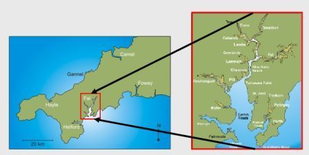
The Fal estuary, located in southwest Cornwall at latitude 50º09’N longitude 05º05’W, formed as a ria (drowned river valley) between 10,000 and 17,000 years ago. It is the third largest deep water harbour in the world and is categorised as a major port by the Department of Environment, Food and Rural Affairs (DEFRA). The main body of the estuary is classified macrotidal with maximum tidal range of 5.3m, and the upper regions are classified mesotidal. Mean coastal water temperature is 16ºC in the summer, immediately subsequent to maximal solar input for the year, and is 9ºC during winter. Little freshwater input effect is observed offshore from Falmouth. Prevailing winds in the region are southwesterly.
The Fal Estuary is the most metal polluted estuary in the United Kingdom. The area has been mined for heavy metals such as tin, lead, iron, arsenic, tungsten, uranium, gold and copper. Copper concentrations exceed the environmental quality standards (EQS) by 5µg/l. Subsequent to the closure in 1991 of Wheal Jane, the last mine, a major pollution event occurred in Restronguet Creek. The anthropogenic impact on the Fal has resulted in the area becoming a focus of chemical and biological marine studies. The area is designated a Special Area of Conservation (SAC) due to the presence of extensive maerl beds, seagrass beds (Zostera sp.) and oyster fisheries (classification B). In Restronguet Creek there are now few species, and those remaining are genetically adapted to high heavy metal concentrations. High eutrophication levels have also resulted in the classification of the area as ‘sensitive’ under the European Union Nitrate Directive. Heavy disturbances occur in the Fal estuary due to china clay extraction, dredging and sewage outlets, and shipping related activities have resulted in the release of both oil and antifouling agents such as Tributyltin (TBT). TBT levels exceed the EQS by 2ng/l and TBT pollution has resulted in incidence of imposex in dogwhelk Nucella sp. (Smith, 1971). This website presents the preliminary findings of a geophysical, estuarine and offshore study of the Fal estuary conducted in July, 2008 by marine science students from the University of Southampton. All times are in Greenwich Mean Time (GMT) and all positions in WGS ’84. |
|
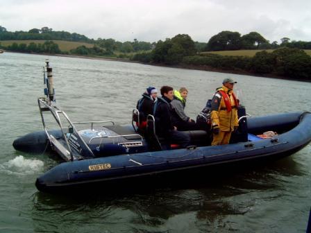
Vessels
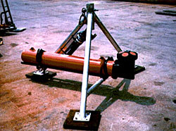
Equipment
|
|
|
|||||||||||||||||||||||||||||||||||||||||||||||||||||||||||
|
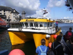
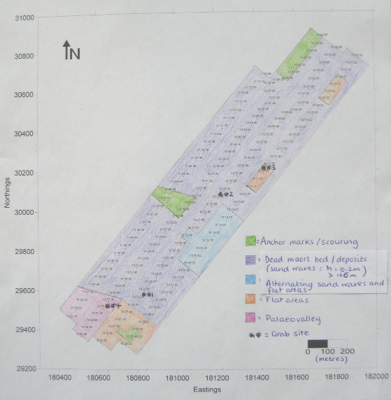
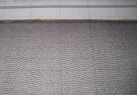
Introduction On Thursday 4th July 2008, a geophysics investigation into the benthic habitat of Falmouth Bay was carried out from the vessel R/V Xplorer between 0900 and 1500. The area surveyed was between Black Rock and Rosemullion Head, within the SAC boundary. Natural England are involved in the protection of this area, and the data collected may be of benefit to them as part of a baseline study for environmental change over time. Aim: To investigate seabed surface types and features in Falmouth Bay, and the benthic macrofaunal community composition.
Results and Analysis
Conclusion
|
|||||||||||||||||||||||||||||||||||||||||||||||||||||||||||
|
|
||||||||||||||||||||||||||||||||||||||||||||||||||||||||||||||||||||||||||||||||||||||||||||||||||||||||||||||||||||||||||||||||||||||||||||||||||||||||||||||||||||||||||||||||||||||||||||||||||||||||||||||||||||||||||||||||||||||||||||||||||||||||||||||||||||||||||||||||||||||||||||
|
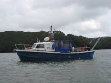
Introduction On Monday 7th July an estuarine practical was carried out on the Fal investigating nutrient concentrations, physical parameters (such as temperature, salinity and flow velocities) and taxonomic identification of phytoplankton and zooplankton. This was achieved by dividing into two groups, one of which sampled the upper reaches from King Harry Reach to Malpas point onboard R/V Ocean Adventurer and a second group doing transects across the main body of the estuary using R/V Bill Conway. Aims:
Tides:
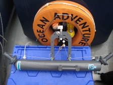
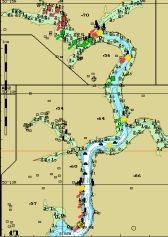
R/V Ocean Adventurer: The upper parts of the estuary were sampled using R/V Ocean Adventurer as R/V Bill Conway could not reach them. Six locations were selected equidistantly apart, ranging from King Harry Passage to Malpas Point. At each location a T/S probe was used to sample the physical structure of the water column. Next, a surface water sample was collected with a handheld Niskin bottle for nitrate, phosphate, silicate and chlorophyll concentrations. These were prepared onboard for later lab analysis by filtering the collected water through a glass fibre filter to extract any suspended particulate matter. At three of the stations dissolved oxygen specimens were also prepared in glass bottles and then stored in water. At King Harry Reach and Malpas point a plankton net was deployed from the stern for ten minutes and formalin added to the collected sample to preserve it for later taxonomic identification. In addition, a measure of each sample was stored in Lugols at every location.
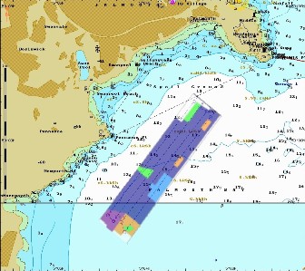
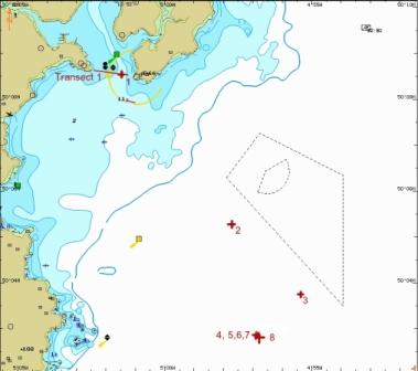
Table showing the 6 stations visited during estuarine sampling using the rib (the yellow diamonds).
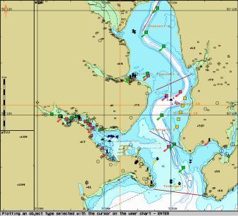
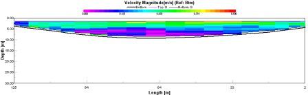
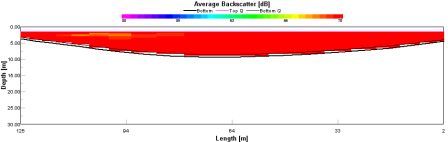
R/V Bill Conway: The coordinates of the start of line (SOL) and end of line (EOL) of each transect line were plotted on Navifisher. Once on the start of line, time and position readings were taken along with a surface water sample (for chlorophyll analysis). A further two water samples were taken along each transect line: one in the middle of the line with time and position readings; and another at the end of the transect line, again with time and position readings. Along each transect line the ADCP was taking constant readings of current velocities and directions in the water column. These values were continually being recorded on hard disk for later processing.
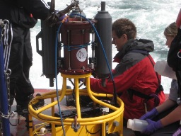
CTD Casts Along each transect line, points of interest were noted of where to take a CTD cast to see what was happening in the water column below. These points were decided where there were significant influences in the composition of the estuarine waters. These influences included the effect of treated sewage diffusers and the effect of rivers entering the estuary on nutrients levels. When on station, time and position were noted down when the CTD was lowered into the water. It was then sent down close to the seabed taking temperature, salinity and depth values on the way down to gauge where water samples were to be taken on the ascent back to the boat. The Niskin bottles were fired at the bottom, middle and top of water column. Water Sampling Once the CTD was returned to the boat deck, sub-samples of the water in each Niskin bottle was taken. Firstly, the preparation of dissolved oxygen analysis samples was carried out. Two reagents were added to the glass bottles containing part of the water sample, and the lids placed on to make sure there were no air bubbles. The bottles were then placed in a bucket of water to prevent the seals from drying out and letting oxygen in the water sample escaping. For preparation of the phosphate and nitrate samples, (after rinsing) 40ml of sample was filtered through a syringe into bottles for later analysis in the lab. This process was then repeated for the silicate samples but using plastic bottles. The filter was then removed from the syringe and placed inside a labeled tube of acetone for later chlorophyll analysis. Another 50ml of the sub-sample was taken up in the syringe, a new filter attached and filtered into a brown bottle. In addition, part of the sample was placed in a bottle containing Lugols Iodine solution in order to preserve phytoplankton for microscope analysis. This method was repeated for each fired Niskin bottle and all bottle numbers and corresponding depths, temperatures, salinities, times and positions were noted down in a table.
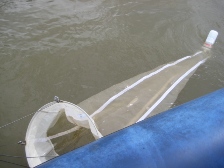
Sampling on the RIB During two transects, a zooplankton net was towed behind the vessel at approximately 4 knots for one minute. As the net was put in and out of the water, time and position were noted along with the reading on the torpedo meter. The sample bottle was unscrewed from the net and formalin added to the sample to fix the plankton and to prevent any changes in their numbers before lab analysis. The readings from the torpedo metre show revolutions of the torpedo whilst being towed, along with the speed the net was being towed at; the amount of seawater sampled can then be calculated. At each CTD sampling station, the depth of the euphotic zone was analysed by lowering a secchi disk in the water column and observing at which depth the disk disappears. Also, at each CTD cast station the speed and direction of the wind was measured by holding an anemometer in the direction of the wind as far over the side of the vessel.
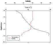
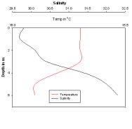
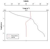
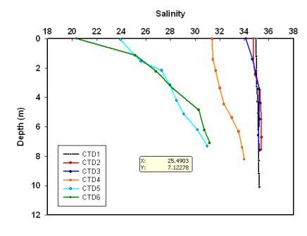
Physical structure: CTD:
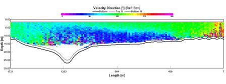
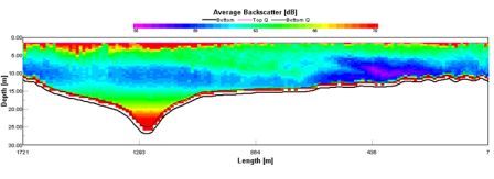
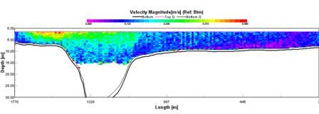
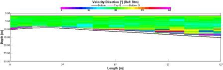
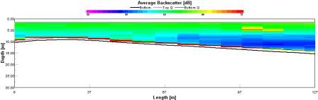
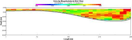
ADCP:
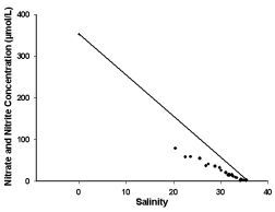
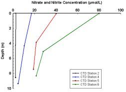
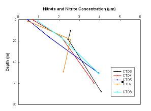
Nitrate
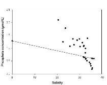
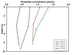
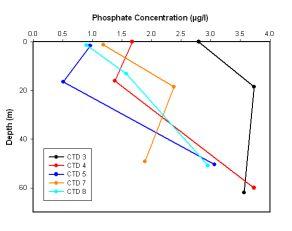
Phosphate
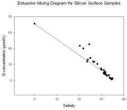
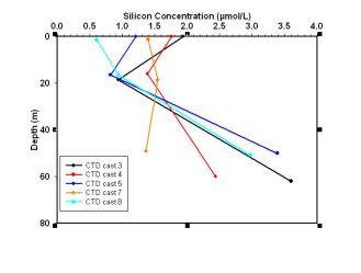
Silicate
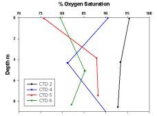
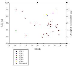
Dissolved Oxygen
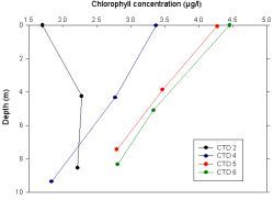
Chlorophyll
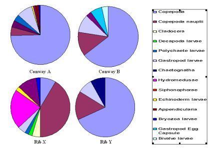
Plankton >Zooplankton
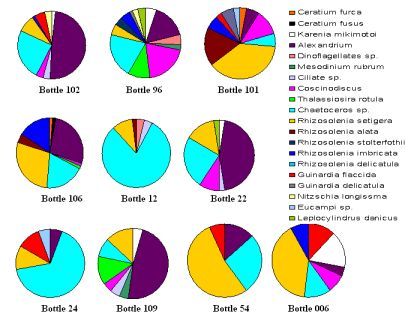
>Phytoplankton
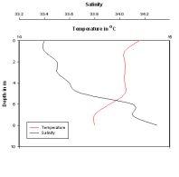
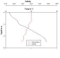
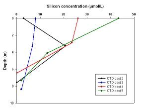
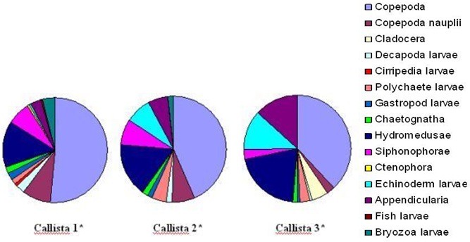
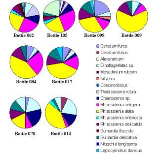
Variation was observed in the physical structure of the water column along the salinity gradient, with slight stratification observed at the mouth of the estuary increasing to strong stratification as salinity decreased up the estuary, reflecting the tidal domination and salt wedge character of the estuary. Nutrient concentrations also showed variation along the salinity gradient decreasing from maxima at low salinities to minima at high salinities, and with depth reflecting dilution of riverine input. Nitrate showed non-conservative removal suggesting uptake by phytoplankton, and phosphate showed non-conservative addition in the upper in the mid-estuary and removal in the lower estuary suggesting inputs of sewage and uptake by phytoplankton. Silicate showed non-conservation addition suggesting inputs from resuspension of the sediment or dissolution of dead diatom frustules Chlorophyll concentrations decreased from maxima at low salinities to minima at high salinities, and with depth suggesting observed stratification and nutrient gradients were responsible. In contrast oxygen concentrations increased from minima at low salinities to maxima at high salinities suggesting bacterial activity, possibly associated with sewage inputs, causing removal of oxygen in the upper estuary. The absence of an observable trend in oxygen concentration with depth suggests variation in the bacterial populations possibly due to proximity to point sources of sewage discharge. The observed variation in composition of phytoplankton population is strongly linked to the observed variation in nutrients. In the mid-estuary high silicate concentrations allow diatom populations to dominate with a shift to dinoflagellates dominating in the lower estuary. Variation in composition of zooplankton population is strongly liked to the observed variation in salinity. Copepods and copepod nauplii dominate the zooplankton population suggesting strong tolerance to salinity and temperature. |
||||||||||||||||||||||||||||||||||||||||||||||||||||||||||||||||||||||||||||||||||||||||||||||||||||||||||||||||||||||||||||||||||||||||||||||||||||||||||||||||||||||||||||||||||||||||||||||||||||||||||||||||||||||||||||||||||||||||||||||||||||||||||||||||||||||||||||||||||||||||||||
|
|
||||||||||||||||||||||||||||||||||||||||||||||||||||||||||||||||||||||||||||||||||||||||||||||||||||||||||||||||||||||||||||||||||||||||||||||||||||||||
|
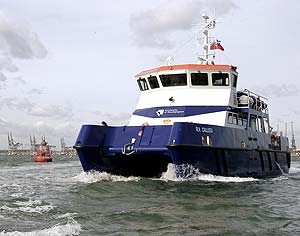
On Thursday 10th July RV Callista set out at around 08:30 GMT from Falmouth Harbour to an offshore location 6 miles due South East. Often in the summer when there is more pronounced stratification of the water column, tidal mixing fronts occur. These are caused by the upwelling of the permanent thermocline as the seabed shallows towards the shore which causes two distinct layers. Due to their dependence on light, phytoplankton are located in the warm well mixed upper layer of the water column, where they utilise and reduce the levels of nutrients present. The isolated cooler water below lacks phytoplankton and thus has higher levels of nutrients present. As the thermocline upwells, the cooler water with higher nutrients is raised to the surface allowing a stronger phytoplankton bloom to develop. This change in water column type allows detection of the location of the tidal front via temperature changes and possible colour changes caused by phytoplankton blooms. Aims
Tide Table (10/07/2008)
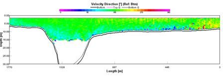
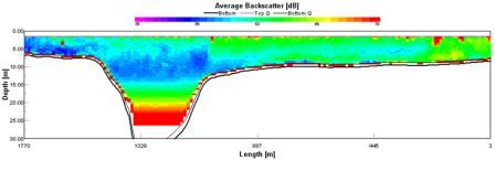
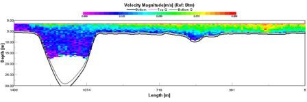
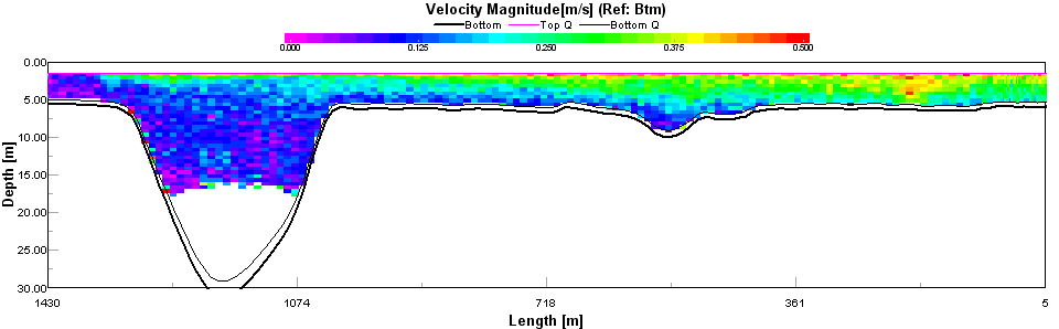
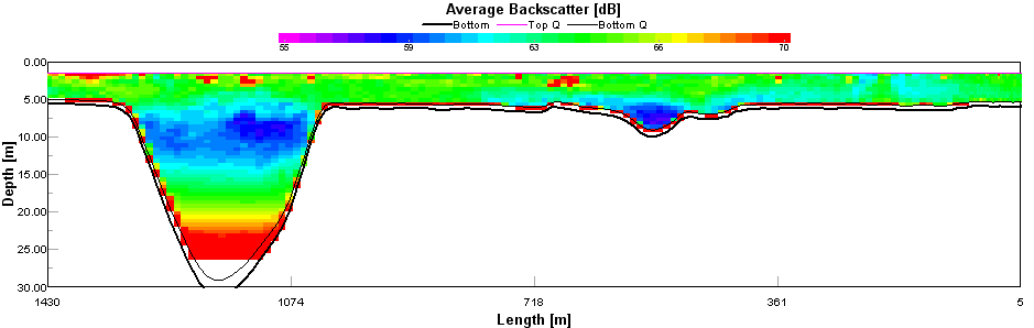
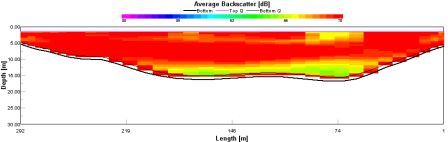
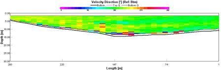
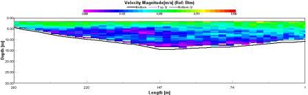
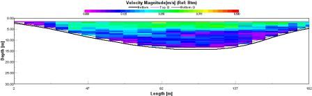
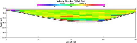
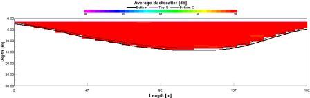
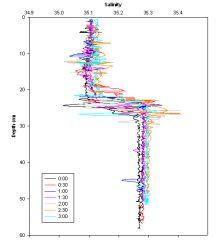
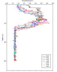
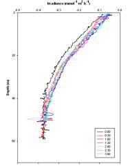
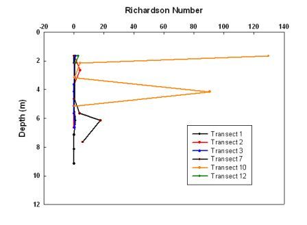
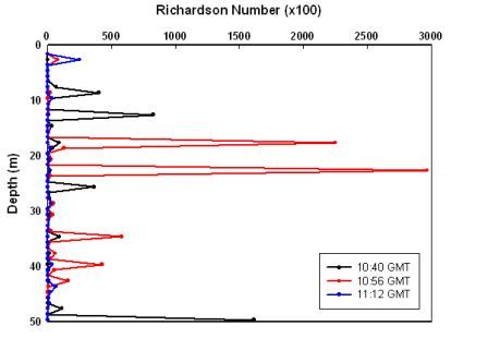
At Black Rock an ADCP transect was performed across the estuary mouth from Shag Rock on the North East side to Pendennis Point on the south west side. From Black Rock, we traveled due south east, running the thermosalinograph to observe changes in the surface waters temperature and salinity. A sharp rise in salinity would indicate a tidal front. Sampling was planned to be carried out on the offshore side of the front, where the water column is more stratified. From the thermosalinograph readings, station 4 was selected 6 miles offshore and the anchor was dropped. A CTD cast was deployed to provide a vertical profile of the water column showing that we were suitably located in the offshore side of the tidal front due to evidence of water stratification. CTD CTD casts were performed on our way out to our offshore station, firstly at Black Rock; in the middle of our first transect across the mouth of the estuary to gain a comparative view of the nutrient, oxygen, chlorophyll and phytoplankton levels in the estuary to our offshore station. Two more subsequent casts were performed on our way out at increasing distances from the coastline to gain a view of how the levels already mentioned were changing with water depth and encroaching onto more and more stratified waters. Once on station 4, 6 miles offshore, CTD casts were performed every half hour, including one undulating cast where the CTD was lowered to the sea floor and bought back up the surface 5 times. With these casts temperature, salinity, fluorescence and logged irradiance were recorded. A record of temperature enabled us to identify a thermocline (if present) to correlate to chlorophyll maxima and potentially minimas in nutrient levels due to uptake by phytoplankton. ADCP During deployment of the CTD cast, the ADCP was run to provide information on the structure of flows in the water column. Comparing velocity readings at different depths allows shear to be identified and the Richardson Number to be calculated. Backscatter results were also used to show turbulence in the water column and the presence of zooplankton blooms. This data was also used onboard RV Callista to decide on the location of zooplankton sampling. Thermosalinograph After performing our ADCP transect from Shag Rock to Pendennis Point (along with the CTD cast at Black Rock); we steamed due south east to our offshore location. Whilst travelling we ran the thermosalinograph which was to continually sample the surface waters as we travelled out. The purpose of this was to observe an increase in temperature and a drop in salinity, whereby this would then identify the tidal front. Evidence from the thermosalinograph data instead showed a slow shift from a well mixed estuarine system to a stratified water column system with no real evidence of a well mixed area, being the inshore edge of the tidal front. Water Sampling From the sea floor to surface of each CTD cast, the three Niskin bottles (9, 7 and 5 respectively) attached to the rosette were fired, acquiring water samples at each level. Bottle 9 was fired at the sea floor, bottle 7 in the mid water-column around the chlorophyll maxima; and bottle 5 at the sea surface. Oxygen Once the CTD was back on deck, the first samples taken from each Niskin bottle was for oxygen into the clear glass oxygen bottles. It was ensured that there were no bubbles inside the sample bottles as any trapped air bubbles will alter the true values of oxygen in the bottle. Back in the wet lab on Callista 1ml of manganese chloride was firstly added to each water sample bottle with a hand pipette followed by 1ml of alkaline iodide. Each lid was replaced onto its respective bottle on an angle as to ensure no air bubbles were trapped under the lid. Each bottle was then inverted to mix the chemicals with the water sample and then submerged in water in a cool box. The bottles were submerged to prevent the seals around the lid from drying out and any extra oxygen entering the water sample, altering the final value when analysed. Oxygen was sampled first because once the tap is opened; the sample is in effect contaminated with atmospheric oxygen, potentially altering the oxygen make up of each water sample. Nitrate, Nitrite, Phosphorous and Chlorophyll Once the sample for oxygen was taken directly from the Niskin bottles, a 1litre sub-sample from each bottle was then taken and transported back into the wet lab. From this sub sample, 50ml was measured in a measuring cylinder and placed into a syringe with filter attached to the end. This 50ml sample was then passed through the filter into a numbered brown glass bottle. The filter from this filter holder was then placed into a refrigerated numbered tube of acetone for later chlorophyll analysis back in the chemistry lab. Silicate and Chlorophyll From this 1litre sub-sample, another 50ml was measured out into a measuring cylinder and placed into another syringe with a new filter attached to it. This 50ml of sample was then passed through the filter and into a plastic numbered sample bottle. This silicate sample must be stored in a plastic bottle because glass contains silicate and would therefore alter the silicate levels in the water sample by leaching silicate from the glass. The filter holder was then detached from the syringe and the paper filter within was placed into another numbered tube of acetone for later chlorophyll analysis back in the chemistry lab. Lugol From each Niskin bottle 1litre subsample, 100ml was measured out with a measuring cylinder into a numbered tall brown bottle containing 1ml of lugols iodine solution. These lugol bottle samples were for later phytoplankton analysis back in the chemistry lab. Closing net Closing net samples were taken in conjunction with the data received from the backscatter output on the ADCP readout. A maximum in backscatter shows a peak in zooplankton abundance in the water column. Closing net samples were taken at station 1, where the net was lowered down to 14m in the water column in response to a backscatter maxima on the ADCP readout. The net was bought up from 14m to surface (the upper limit of the backscatter maxima) where it was then closed. The net was then brought back onto deck where it was washed from the outside so all zooplankton collected were washed down into the collection bottle attached to the bottom of the net. The sample in this collection bottle was transferred to a labelled 1litre plastic bottle along with a large measure of Formalin to kill and fix all the zooplankton, preventing their numbers from changing within the sample. This procedure was then repeated at station 5 with two closing nets, one from 27m up to 18m (the thermocline) and one from 10m to 0m. These sample sites were selected in response to backscatter maximums in the ADCP readout data. Secchi Disk At each station where a CTD cast was performed, secchi disk analysis of the euphotic zone was performed. This was done by lowering the secchi disk over the edge of the vessel down into the water column and observing it until it disappeared. An average level on the line attached to the disk was marked by eye, average due to the fact there was a large swell which travelled up and down the line, affecting the true value of the euphotic zone. The secchi disk was then returned to deck where the length of the line was measured and multiplied by three to gain the lower limit of the euphotic zone at that station. It was also noted that the secchi disk was being lowered from the deck of considerable height from the true sea level, and corrections were made to account for this fact. All values of secchi depth were noted down along with positions of sample sites.
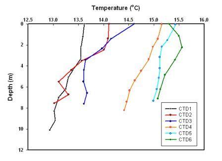
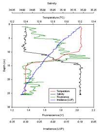
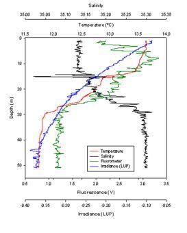
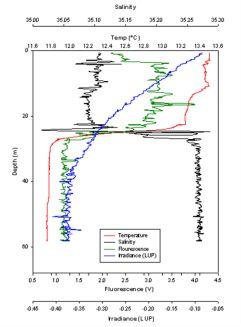
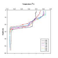
Results and Analysis CTD
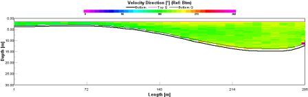
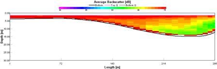
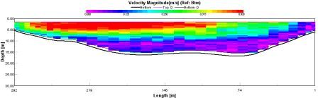
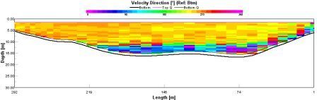
ADCP:
Nitrate
Phosphate
Silicate
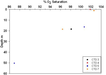
Dissolved Oxygen
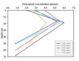
Chlorophyll
Zooplankton
Phytoplankton
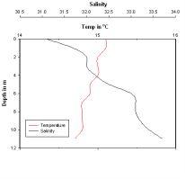
At the mouth of the estuary there was no stratification seen, however at our offshore location clear stratification can be seen. A thermocline and halocline were constantly present at 25-30 metres with the chlorophyll maximum fluctuating around 15 metres. Throughout the time series analysis there was only slight variations in these depths and this was caused by an internal wave. Apart from this internal wave the water column was fairly stable, shown by the Richardson number values all being over 1.These values were obtained from the ADCP data. Whilst the water column remained stable, surface waters did warm slightly over the duration of the day, due to the decreased cloud cover. Chlorophyll concentrations at the chlorophyll maximum were at least 1µmol/l higher than the surface levels. Phytoplankton abundance in the surface waters was lower than that of the chlorophyll maximum due to the depletion of nutrients. Low concentrations of nutrients in the surface waters support this. Phosphate levels were high at deeper waters where consumption would be lower due to the fact that photosynthesis at such deep depths cannot occur as it is outside of the euphotic zone. Overall the site sampled was both too deep and too far offshore to be significantly affected by tidal mixing and wind driven mixing. As a result stratification occurs leading to the presence of a thermocline and hence the chlorophyll maximum.
|
|
We have created this web page as a summary of our finding, which are all available to download from the University of Southampton FTP website. This was only a short investigation in the local area, with further study required to gain a full data set. We are aware that there are limitations to our findings over tidal cycles and seasonal variation. We would like to thank all the staff and demonstrators for all the time, effort and support they provided during this fieldwork course. The views expressed in this website do not neccessarily represent those of the University of Southampton or the National Oceanography Centre, Southampton. |
|
Dyer, KR: (1997). Estuaries, a physical introduction (2nd edition). John Wiley and sons ltd. Chichester. Knauss, JA: (2005). Introduction to physical oceanography (2nd edition). Waveland Press inc. USA. Miller, C B (2004) Biological Oceanography. Blackwell publishers, Singapore. Parsons, TR; Maita, Y; Lalli, C. (1984) A manual of chemical and biological methods for seawater analysis 173 p. Pergamon. Langston, W. J., Chesman, B. S., Burt, G. R., Hawkins, S. J., Readman, J., Worsford, P. 2003. The Fal and Helford; characterisation of European Marine Sites. www.deepsea.co.uk/boats/xplorer www.soes.soton.ac.uk/resources/boats/vessels.html Local area weather forecast [accessed online, July 2008]: http://www.metoffice.gov.uk/weather/uk/sw/sw_forecast_weather.html
|