F A L M O U T H F I E L D C O U R S E 2 0 0 8
~ Group 5 ~
Buckle. N, Carrick. D, Harris. J, Hartle-Mougiou. K, Kaack. B, Lew. S, McCorquodale. S, Molloy. L, Herron. J, Ziesler, S
![]()
![]()
![]()
![]()
![]()
![]()
![]()
![]()
INTRODUCTION
As second year oceanography students we were set the task of investigating the physical, chemical and biological properties of an inshore estuarine and offshore environment. We travelled to Falmouth, Cornwall, to study the Fal estuary. This site aims to provide the reader with a detailed description of the investigations conducted from the 1st to the 12th of July including information regarding aims and objectives, investigation protocols describing equipment used, results obtained and an analysis and discussion of results.
|
Estuaries have long been researched due to their ecological importance. This is owed to a diverse range of habitats and biodiversity due to spatial and temporal changes in chemical and physical gradients. They are also important transition zones of minerals and materials from terrestrial to marine environments.
The Fal Estuary,
|
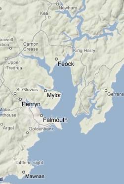 |
The Fal estuary has a rural water catchment derived from arable and dairy agriculture and reflects the underlying geology: Carnmellis granite and metamorphic rocks. Mining processing of metalliferous deposits since the Bronze Age to modern day (1992) has led to increase in metal concentrations within the sediments and overlying waters. Moreover, high inputs of organic matter (sewage) and nutrients have led to eutrophication in the upper Fal. The Fal supports a wide range of communities including the largest Maerl bed in South West England as well as diverse epifaunal and infaunal communities, described as a Primary Site of Natural Marine Biological Importance by Bishop and Holme (1980). Furthermore, as a result of the anthropogenic perturbation it has been designated as a Special Area of Conservation (SAC) and defined as ‘Sensitive Areas’ under the Nitrate Directive (91/676/EC). |
~ Back to top ~
|
Technical specification and
dimensions: |
R.V. Callista |
Ship’s equipment: |
|
Length
overall: 19.75m
Speed: 14-15Kts, range 400nm |
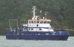 |
“A” frame and associated winch – 4 tonne lifting capacity, 150m x 14mm cable |
| R.V. Bill Conway | ||
|
Length overall: 11.74m |
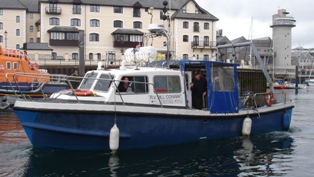 |
Simrad Navigation computer. |
| Ocean Adventure RIB | ||
|
Length overall:
7.00m |
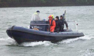 |
Hull Ribtec 700 |
| Xplorer | ||
|
Length overall: 12.00m |
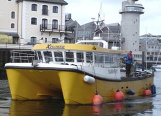 |
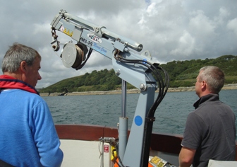
Heila deck crane with winch |
~ Back to top ~
|
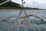
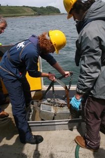
Van Veen Grab |
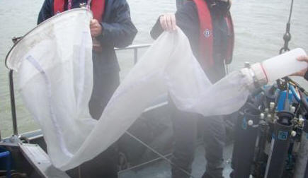
Plankton Nets & Flow Meter |
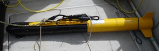
Towfish |
|
|
 |
 |
|
The Van
Veen grab is designed to collect samples of
the seabed. The contents can then be analysed according to biotic
composition and grain size by sieving through various mesh sizes. |
These mesh nets have a spacing of 200µm to collect zooplankton in the water column. As the net is retrieved the contents are pushed towards the collecting bottle attached to the bottom of the net. The flow meter is a 3-blade impellor connected to a 5 digit counter. The counter records each revolution of the impellor. |
The Towfish is a torpedo shaped Geoacoustic sidescan instrument with a mounted transducer that emits a fan shaped acoustic pulse between 100KHz – 500KHz whilst being towed subsurface behind the boat. It is used to define bathymetric features. |
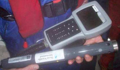
| YSI Probe |
Niskin bottle |
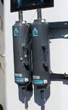
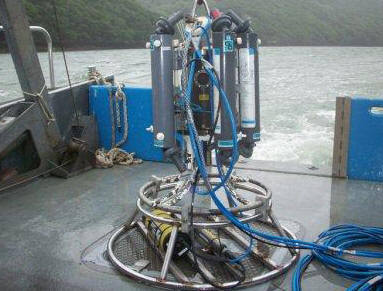
CTD and CTD rosette |
 |
 |
 |
|
This multi parameter probe can be lowered by a simple cable manually and is used to generate a vertical profile of various parameters, including; temperature, salinity and chlorophyll. |
These bottles collect water samples at predetermined depths. Sub-samples can also be taken from the bottles for further analysis. The bottles are attached to either a hydroline or a CTD rosette. |
The CTD is a multi parameter platform capable of continuously recording temperature and salinity with depth. Additional instruments that can be attached include; a fluorometer, Niskin bottle(s) and a transmissometer. |
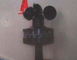
| Secchi disk | Acoustic Doppler Current Profiler (ADCP) | Anemometer |
 |
 |
 |
|
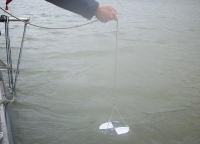
This simple black and white circle is lowered by hand into the water column until the colours can no longer be distinguished. The attenuation coefficient and depth of euphotic zone can then be calculated. |
This is used to measure the speed and direction of currents within the water column and can be mounted on the hull of a vessel. |
An accurate reading of wind speed can be obtained by using this equipment. Simply hold it in front of yourself into the direction of the wind and record off the highest value. |
~ Back to top ~
General Information
| Date: | 09/07/2008 |   |
| Vessel: | R.V. Callista | |
| Skipper: | Graham | |
| Crew: | Nigel and Gary | |
| Demonstrator: | Duncan Purdie | |
| Area surveyed: | Falmouth Bay | |
| Equipment Used: | CTD rosette with niskin bottles attached | |
| ADCP | ||
| Plankton nets | ||
| Secchi disc | ||
| General Weather Notes | Cloud cover | Wind | Pressure (mb) | Temperature (oC) | ||
| Direction | Speed (knots) | Air | Sea Surface | |||
| Spells of heavy and light rain throughout day | 8/8 | SSW | 10-30 (mean 17.4) | - | 16 | 12-13 |
Aim
The aim of this practical was to investigate the influence of vertical mixing processes on the distribution and properties of phytoplankton and nutrients offshore.
|
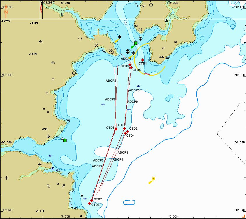
Click to enlarge |
Methods |
|
Fig 1.1 Chart showing location of transects and sample sites. |
|
Chemical procedures and analysis
The water samples were analysed in a laboratory for the chlorophyll, dissolved Phosphate and Silicon concentrations using the method described by Parsons et al (1984). Dissolved oxygen was calculated following the Winkler method described by Grasshoff et al (1999). Nitrate concentrations were measured by Flow injection analysis as described by Johnson and Petty (1983).
Phytoplankton analysis: 100ml of solution in the lugol iodine glass bottles were left to settle. The top 90ml were then removed using a pump concentrating the sample to 10ml. 1ml of this sample was put into a gridded Sedgewick Rafter counting cell and studied under a microscope.
Zooplankton analysis: A sample was inserted into a Bogorov chamber and studied under a microscope.
Results
Vertical Nutrient Profiles
|
Silicon: All stations show similar concentrations (below 3μmoll-1). Station 7, however, shows a marked increase compared with other stations and a maximum of 6.835μmoll-1 at a depth of 11m.
|
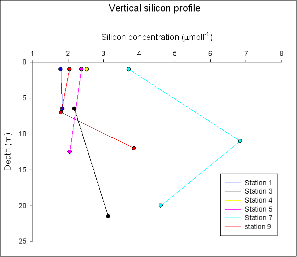 Fig 1.2 Silicon vertical profile |
|
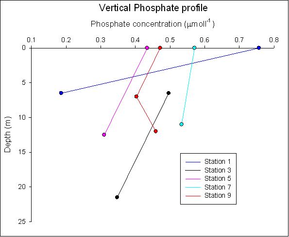
Phosphate: All stations have a concentration below 1μmoll-1 at all depths. These low concentrations are likely to be due to the increased distance from land (compared to our estuarine samples) causing the nutrient input from terrestrial sources to be greatly reduced. The input of recycled nutrients will therefore have a larger affect on the over-all concentrations. The removal of nutrients by phytoplankton and the low nutrient inputs caused the resulting reduced phosphate concentrations. |
Fig 1.3 Phosphate vertical profile |
|
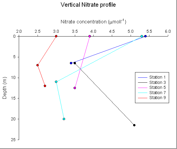
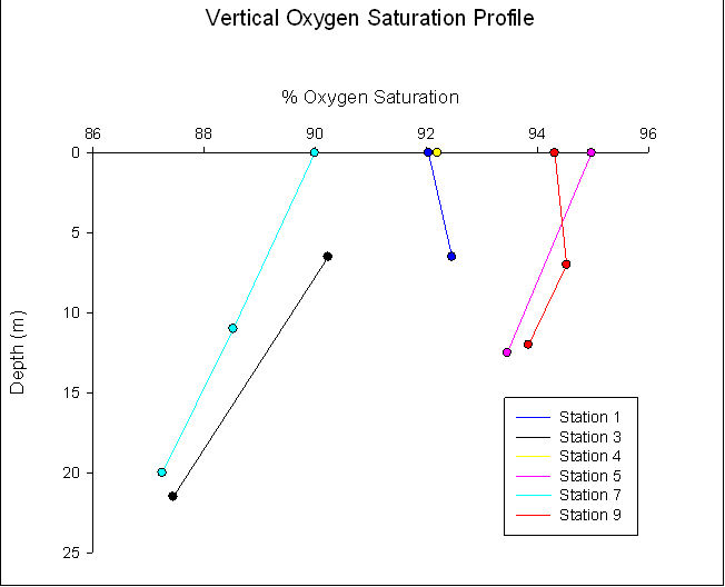
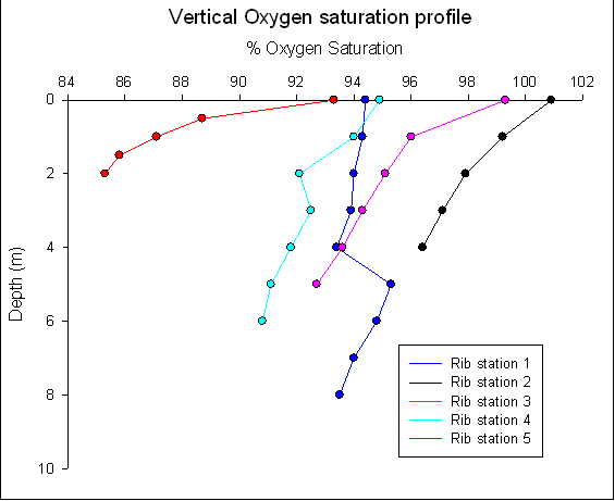
Nitrate: Stations 3 and 7 show a marked decrease in oxygen saturation compared to the other stations, possibly due to their sheltered location behind a headland. Consequently there was a reduction in wave size in the area, and hence a smaller surface area of the sea surface/air interface, possibly accounting for the reduction in % saturation. |
Fig 1.4 Nitrate vertical profile |
|
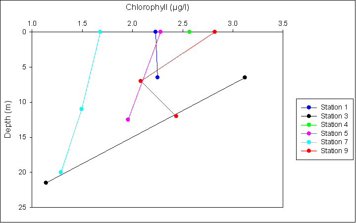
Chlorophyll: In areas with high chlorophyll concentrations, generally have low values of silicon. This is likely to be due to the fact that diatoms are utilizing the silicon, depleting the concentrations in seawater. For example the highest chlorophyll concentration was found at 6.5m at station 3, where there was a silicon concentration of 2.18µmol/l. This trend is not displayed at all stations. Change in chlorophyll with nitrate and phosphate levels shows no clear relationship. There would need to be many more samples and replicates in order to provide an accurate insight into relationship between chlorophyll and nutrients concentrations.
|
Fig 1.5 O2 vertical profile |
|
Dissolved O2: The nitrate concentrations at all the stations show no evident trends. All values fall between the range of 2.5 to 5.5μmoll-1. More data is required to make any conclusive summations about changes with depth or between stations. |
Fig 1.6 O2 vertical profile |
CTD profiles
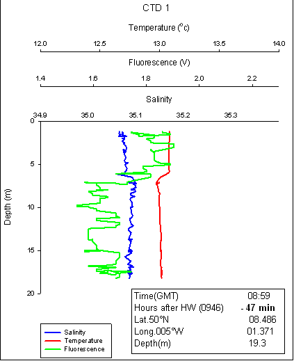
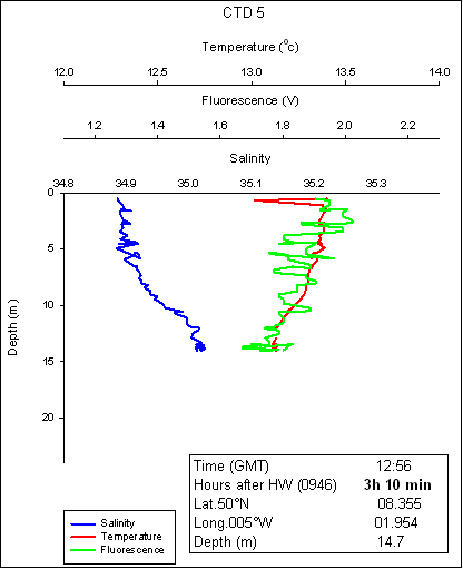
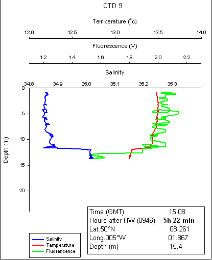
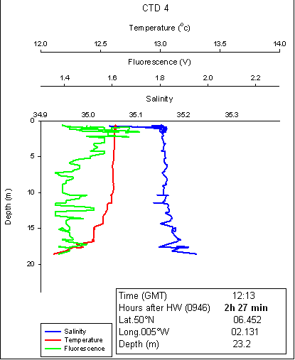
| Station 1 - Black Rock | ||
 |
 |
 |
| Fig 1.13 | Fig 1.14 | Fig 1.15 |
|
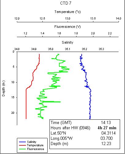
A clear wind driven surface layer exists at high water (Fig. 1.13) to around 6m. A small halocline (0.5) and thermocline (0.2°c) overly a homogeneous section extending to the sea floor. Fluorescence is greatest in this upper layer and shows a decrease below 6m. Theoretically, shear stresses between these layers are low at slack water leading to a static water column. Since sampling took place 47min before HW (Fig. 1.13) low stress is assumed, having the tendency to increase over time as tidal velocities increase. This cannot be verified as no ADCP data for this location exists. It would be expected that shear stress and constant strong SW winds would lead to mixing of the two layers and act to increase water mixing depth. The signal at station 5 (Fig 1.14) and 9 (Fig 1.15), whilst noisy, does not show the stratification seen in 1 (Fig. 1.13) as both thermocline and halocline are far less pronounced. The depth of mixing increases to around 13m at profile 9 (Fig 1.15) as slack water is again approached (38 minutes before Low Water). Clearly the ebbing tide overrides the stratification seen at HW. Overall water temperature increases by around 0.5°c over almost 6 hours, a complete ebbing of tide. The freshwater input signature is weak (0.2 salinity decrease) but present. A small density compensation decrease was seen in raw data but was not plotted here. At this time of year, riverine flux is warmer than the surrounding ocean and to some extent, the effect of this is seen in the data.
|
||
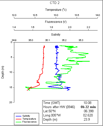
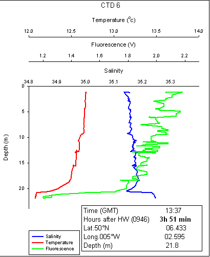
| Station 2 - Middle Station | |||
 |
 |
 |
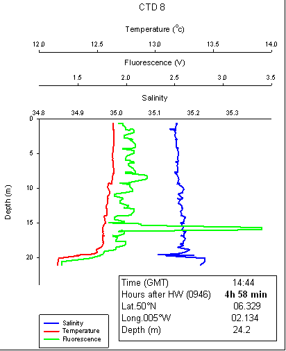 |
| Fig 1.16 | Fig 1.17 | Fig 1.18 | Fig 1.19 |
|
Temperature and salinity show homogeneous profiles with depth at all states of the tide indicating a well mixed area influenced more by wind induced mixing. The effect of tidal currents at this station is masked by this and so interpretation is difficult. Potentially, the Helford riverine flux has an effect on this area. This is subject to seasonal and annual variation and so again it is unwise to draw conclusions from just one data set. A chlorophyll maximum is seen to exist at 15m on profile 8 (Fig1.19). The absence of a front and corresponding thermocline together with the small vertical area in which it exists leads to the belief that this data is erroneous and should not be analysed further.
|
|||
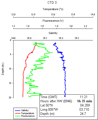
| Station 3 - Porthkerris Cove | |
 |
 |
| Fig 1.20 | Fig 1.21 |
|
Thermo and haloclines appear symmetrical at profile 3 (Fig 1.20) indicating steady slow mixing at this station. This is essentially homogeneous but becoming cooler and more stratified over the 3 hours between sampling. A small dual layer thermocline develops by the second time of sampling (4h 27min post HW). Fluorescence and salinity do not show corresponding changes indicating that the cooler water is arriving from the immediate area and as such has similar nutrient properties.
|
|
Phytoplankton and Zooplankton
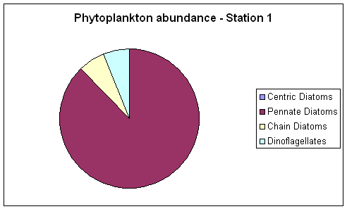
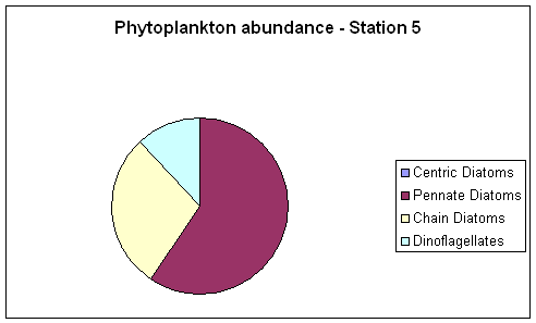
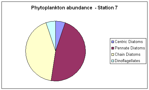
Water samples for phytoplankton analysis were taken at 4 stations (Stations 1, 5, 7 and 9). Diatoms dominated over dinoflagellates with a total number of 60,200 cells per litre and 10,000 cells per litre respectively. Rhizosolenia and Chaetoceros were the dominant genuses found during this offshore survey. Stations 5 and 9 showed the highest and very similar amounts of diatom cells, an expected phenomenon as these two stations are at close proximities to each other. Dinoflagellate species included: Dinophysis genus, Alexandrium genus and Ceratium genus. Highest numbers of dinoflagellate cells were found at station 5. Unlike dinoflagellates, diatoms thrive in mixed waters, so consequently are found in much higher numbers.
At station 7 the lower number of phytoplankton cells is indicative of increased zooplankton activity.
Phytoplankton table of results
 |
 |
 |
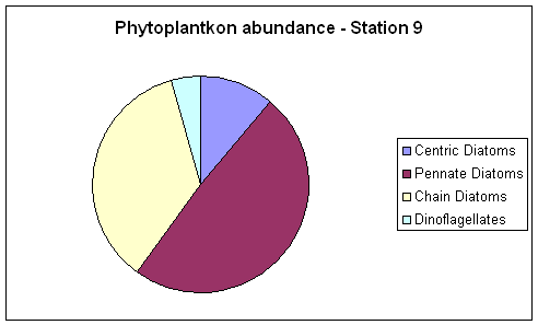 |
| Fig 1.22 Station 1 | Fig 1.23 Station 5 | Fig 1.24 Station 7 | Fig 1.25 Station 9 |
Table 1.1 Pie charts showing proportion of phytoplankton groups present.
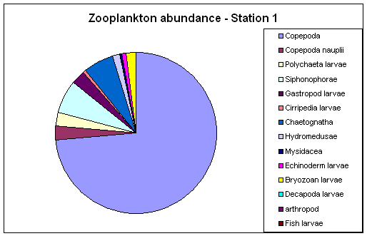
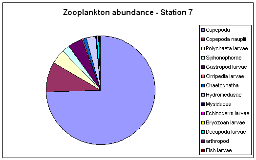
Zooplankton data was collected at 3 stations. Station 1 was situated near black rock (Latitude: 50°08.441, Longitude: 005°01.276) and station 7; near the mouth of the Helford river (Latitude: 50°04.498, Longitude: 005° 03.730). Finally station 9 was also located near black rock although further south than the first station (Latitude: 50°08.292, Longitude: 005°01.823).
All 3 stations were dominated by copepods (See Zooplankton table of results). However, the number of individual copepods per m3 was greatest at station 7 (2591 individuals per m3) and station 1 (914 individuals per m3). Station 7 also showed the greatest diversity of individual species possibly due to the more stratified waters encountered here. CTD station 1 (situated at the mouth of the estuary) was affected by strong flood currents. Alternatively station 9 (also situated at the mouth of the estuary), was affected by ebb flows. Hence zooplankton at both stations found themselves in more stressful conditions owing to the mixed waters. Site 7 also has the lowest chlorophyll concentrations possibly indicating that zooplankton thrives on phytoplankton at this station. Both stations 9 and 1 showed the highest chlorophyll concentrations, indicating a possible bloom due to the limited abundance of zooplankton, and higher nutrient concentrations; transported out of the estuary on the ebb tide.
 |
 |
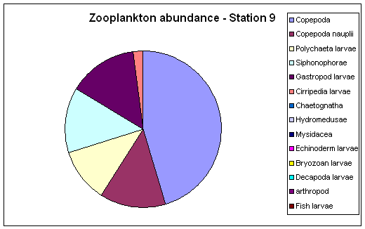 |
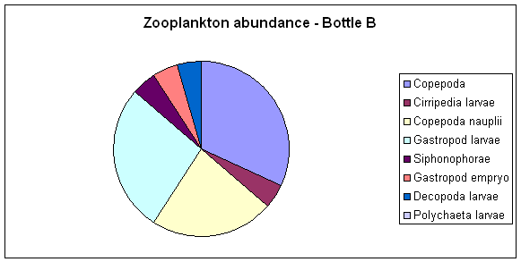
| Fig 1.26 Station 1 | Fig 1.27 Station 7 | Fig 1.28 Station 9 |
Table 1.2 Pie charts showing proportion of zooplankton groups present.
| Dominant Phytoplankton Identified | Dominant Zooplankton Identified |
| Dinoflagellates: Alexandrium and Dinophysis | Copepoda, Gastropoda |
| Diatoms: Chaetoceros, Rhizolenia, Guinardia and Thallasiosara | Polychaetes, Siphonophorae |
Table 1.3 Names of dominant phytoplankton and zooplankton found in our samples. Click on the hyperlinks to view photos taken through the microscopes of particular phytoplankton types.
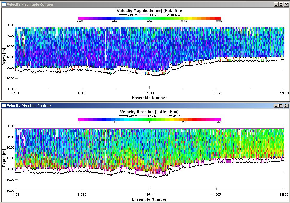
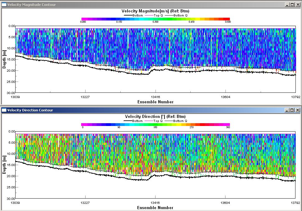
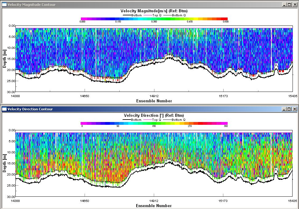
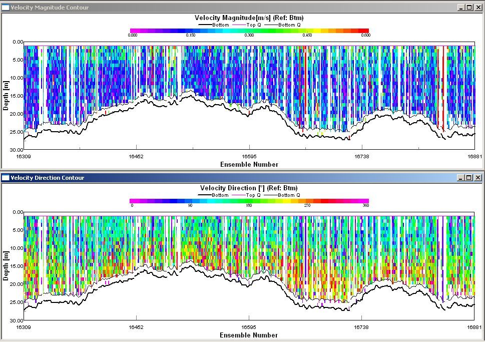
ADCP data and profiles
All ADCP thumbnails below show the magnitude and direction of the flow.
| Transect 1 | Transect 2 | Transect 3 |
 |
 |
 |
|
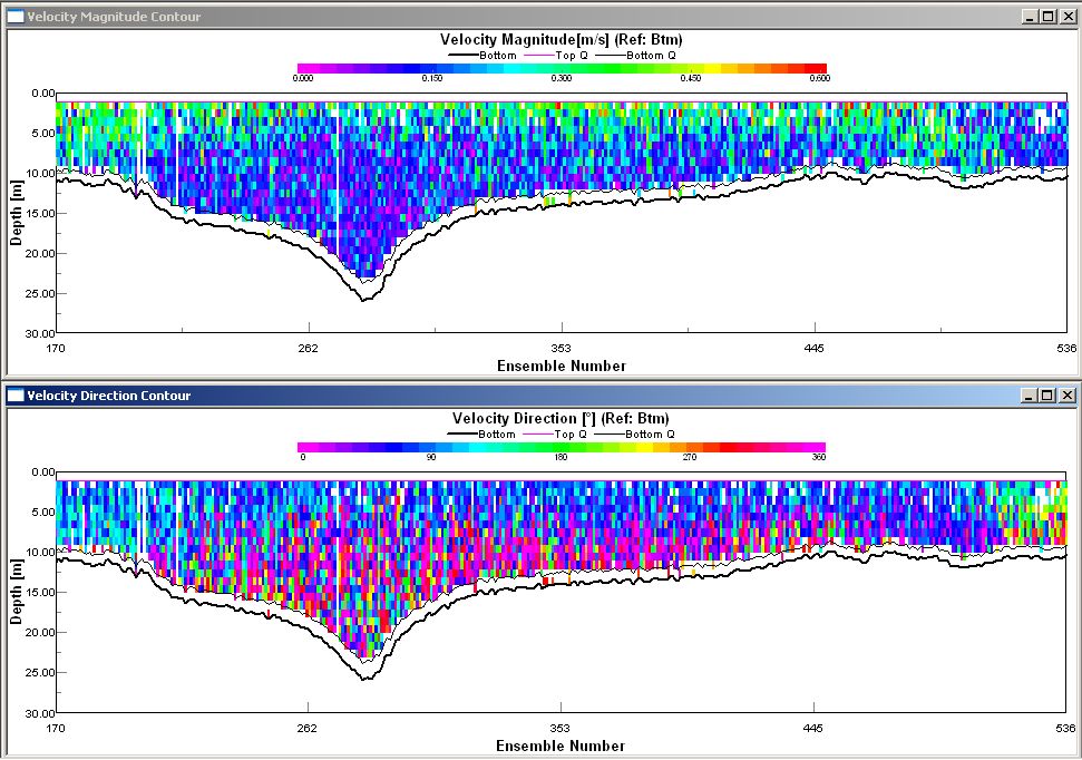
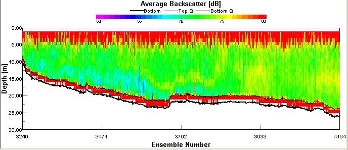
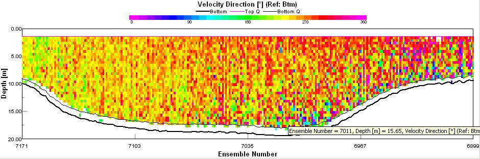
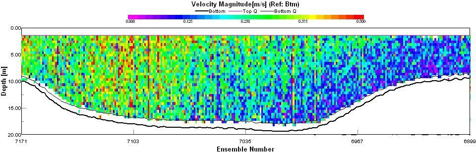
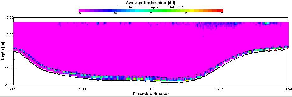
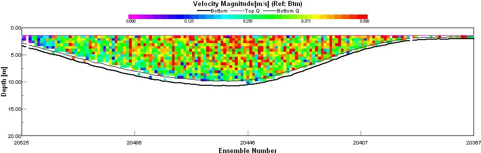
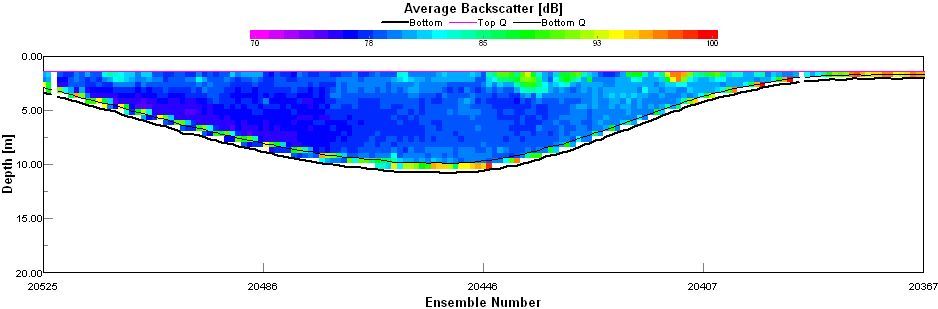
Fig 1.29 Time: 08.38 – 08.46 Length of Transect? 1552m Start Position: 50° 00.369N, 005° 01.816W End Position: 50° 03.673N, 005° 02.367W Velocity direction contour plot – The directional contour plot is of a transect across the mouth of the estuary. The mid depth and bottom waters display a mean northerly flow into the estuary. This correlates with the movement water due to a flooding tide. The transect was taken approximately 1hr before high tide 09.46GMT. Surface waters tend to flow in an in easterly direction, probably a result Ekman transport via strong south-westerly winds. At the far western end of the transect, the water column displays water flow in a southerly direction, possibly explained by the outflow of riverine waters. Velocity magnitude contour plot – The velocity of the flow is greatest near the surface of the water, ~ 0.3m\s. Deeper water is slower, ~0.1m/s, as the tide approaches slack water at high tide. Average backscatter contour plots found nothing of interest in the mid-depths where we were expecting to find increased phytoplankton/zooplankton concentrations. High levels of backscatter were found at the surface due to surface waves producing turbulence. |
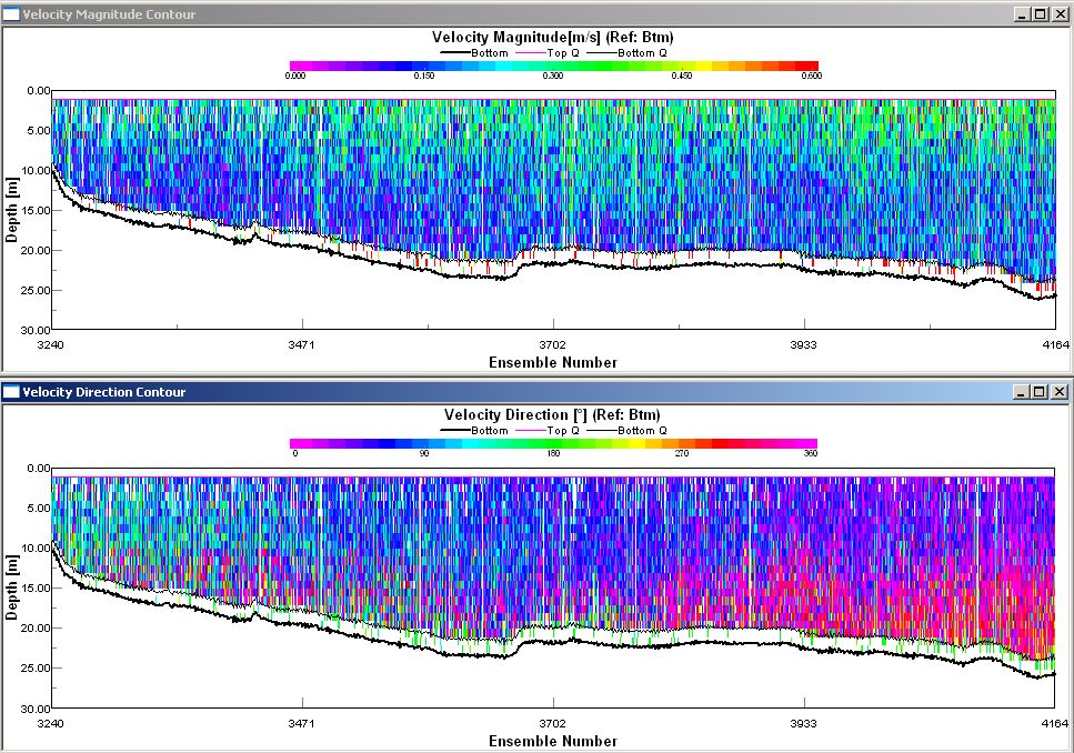
Fig 1.30 Time: 09.45 – 10.05 Length of transect: 3704m Start Position: 50° 08.332N, 005° 02.502W End Position: 50° 06.298, 005° 02.642W Velocity direction contour plot – Transect 2 runs from the mouth of the estuary, in a southerly direction for 3704m. The north end of the transect shows the average direction of net flow in an easterly direction. The south end of the transect has a net flow in a more north-easterly direction. Velocity magnitude contour plot – The time of transect was around slack water, high water (09.46GMT) so tidal currents were minimal. Surface waters ahd an average velocity of approximately 0.3m/s, and the deeper water net flow is slower at approximately 0.15m/s.
|
Fig 1.31 Time: 10.18 – 10.42 Length of transect: 4482m Start Position: 50° 06.522N, 005° 02.587W End Position: 50° 04.108N, 005° 03.929W Velocity direction contour plot – Transect 3 was carried out in a SSW direction, for approximately 4482m and passes across the mouth the River Helford. The north end of the transect displays a a mean net transport in a north-easterly direction. Towards the end of the transect, the direction of flow veers northerly, and then north westerly. These changes in direction may be potential eddying and are mostly likely to be due to the influence of the River Helford and the flooding tide. Velocity magnitude contour plot – Surface layer currents are faster than mid and bottom layers by ~0.15m/s at the start of the transect. The end of the transect sees the magnitude of velocity constant throughout the whole water column (0.1m/s). Average backscatter contour plots were inconclusive, with no areas of interest being highlighted. An increase in backscatter due sediment suspension on the ebbing tide was expected but this was not found.
|
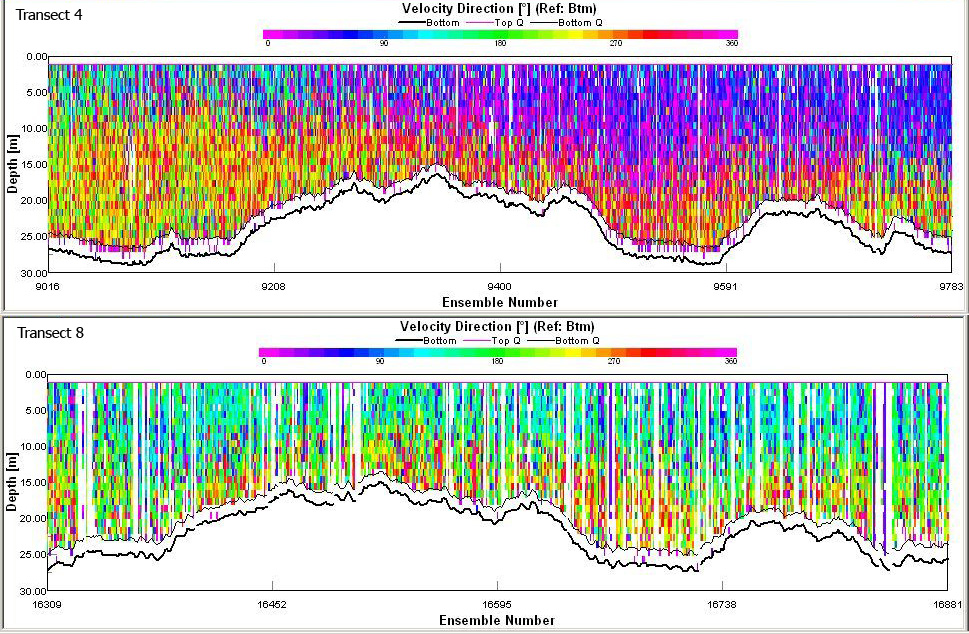
| Transect 4 | Transect 5 | Transect 6 |
 |
 |
 |
|
Fig 1.32 Time: 11.50 – 12.08 Length of transect: 3614m Start Position: 50° 04.441N, 005° 03.513W End Position: 50° 06.454N, 005° 02.194W Velocity direction contour plot – The south end of the transect shows the deeper water flows in a south-westerly direction, following the contour of the coast. Shallower water above this body is moving south-easterly. As the transect moves northwards, the directional flow of the water-column becomes more homogenous and in an easterly direction. This direction is influenced by the ebbing body of water, moving out of the River Helford. Velocity magnitude contour plot – The magnitude of the net flow changes across the transect. The south end has a constant velocity throughout the water column (~0.15m/s), and gradually forms two layers as the transect moves northwards. The surface layers travel ~0.1m/s faster than layers below. The faster moving surface layer is probably the fresher, riverine water moving offshore on the ebbing tide.
|
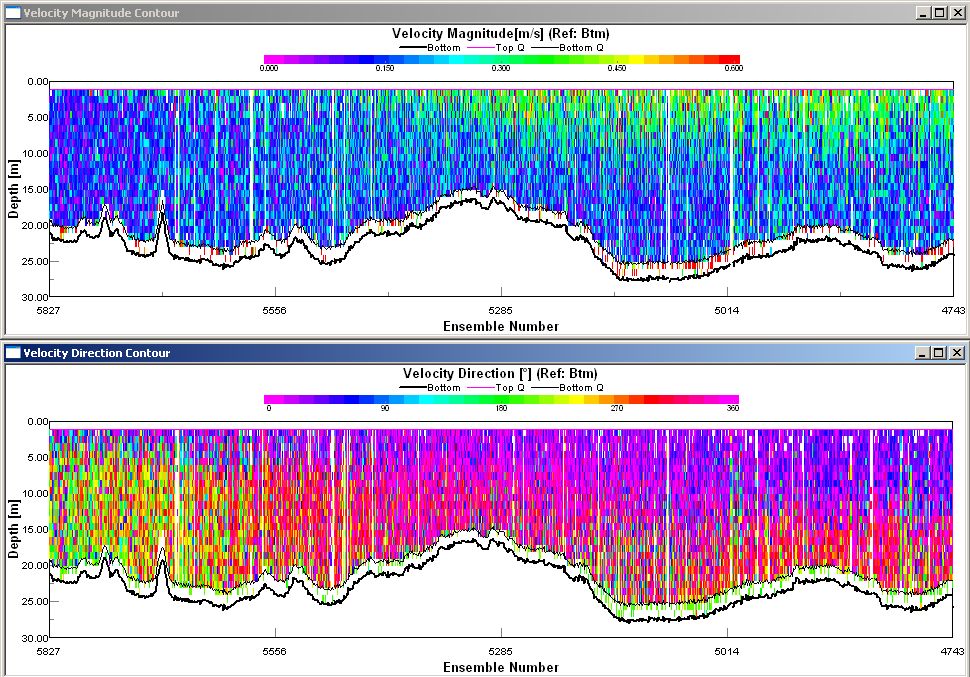
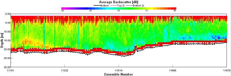
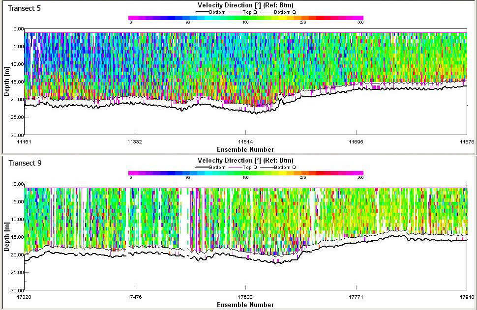
Fig 1.33 Time: 12.37 – 12.53 Length of transect: 3200m Start Position: 50° 06.505N, 005° 02.168W End Position: 50° 08.289N, 005° 01.958W Velocity direction contour plot – The beginning of the transect, in the middle of the bay shows the net transport flowing in an easterly direction. As the transect approaches the mouth of the Fal estuary, the ebbing tide is now evident, with net transport flowing in a southerly direction. The transect was taken approximately 3hr after high tide (09.46GMT), so the ebbing currents are reaching there maximum velocity. Velocity magnitude contour plot – The magnitude is constant across the transect, ~0.2m/s. An interesting area of increased backscatter was found at the beginning of transect 5. This may be a zooplankton bloom at ~ 15m. Areas of high zooplankton concentration often indicate phytoplankton blooms. Zooplankton are migratory so they may be below the thermocline, explaining deeper than usual location.
|
Fig 1.34 Time: 13.19 – 13.35 Length of transect: 3336m Start Position: 50° 08.267N, 005° 02.540W End Position: 50° 06.418N, 005° 02.572W Velocity direction contour – This transect was very noisy and a definitive direction was difficult to identify. The average direction of flow was in a southerly direction with the top 5m of water moving in east. Velocity magnitude contour plot – The magnitude is constant across the transect, ~0.2m/s. The average backscatter contour plot identified a zooplankton bloom ~3.5hrs earlier. Due to the effects of the tides, the bloom was not identified in the second transect of the area.
|
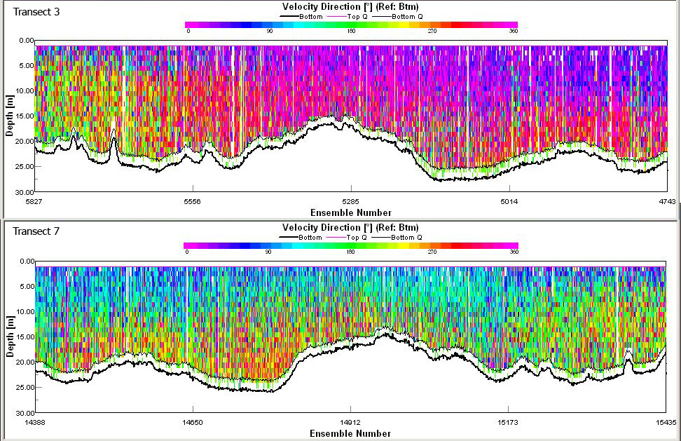
| Transect 7 | Transect 8 | Transect 9 |
 |
 |
 |
|
Fig 1.35
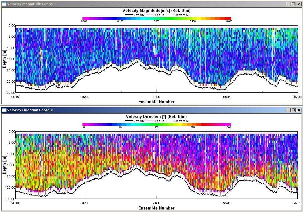
Time: 13.48 – 14.11 Length of transect: 4154m Start Position: 50° 06.457N, 005° 02.587W End Position: 50° 04.293N, 005° 03.854W Velocity direction contour – The water column has split itself into 2 main layers. The upper layer is travelling in n easterly net flow direction, above the lower layers that move in a westerly direction. This induces shear at the layer interfaces and potential turbulence, highlighted by a small increase in backscatter at the correlating depth. Velocity magnitude contour plot – The magnitude is constant across the transect, ~0.2m/s, apart from a small increase in velocity at the surface (0.3m/s).
|
Fig 1.36 Time: 14.30 – 14.41 Length of transect: 3298m Start Position: 50° 04.650N, 005° 03.364W End Position: 50° 06.259N, 005° 02.183W Velocity direction contour – Transect 8 recorded very noisy data with large gaps due to bubbles. The surface layers were moving in a south easterly direction and deep water was moving in a south westerly direction. Velocity magnitude contour plot- Again, the contour plot is very poor due to noisy data. The average magnitude of velocity is ~0.15m/s.
|
Fig 1.37 Time: 14.52 – 15.05 Length of transect: 3183m Start Position: 50° 06.438N, 005° 02.219W End Position: 50° 08.195N, 005° 01.885W Velocity direction contour – Transect 8 recorded very noisy data with large gaps due to bubbles. The surface layers were moving in a southerly across the whole water column. This agrees with the direction of the ebbing tide ( transect taken 5hrs after high water). Velocity magnitude contour plot- Again, the contour plot is very poor due to noisy data. The south end of the transect shows velocity of currents to be 1.5m/s slower than water at the north end of the transect, at the mouth of the estuary. This is due to ebbing water still moving from the estuary.
|
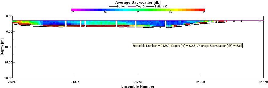
Backscatter plots
 |
 |
|
Fig 1.38 -
Transect 2 Time: 09.45 – 10.05 Length of transect: 3704m Start Position: 50° 08.332N, 005° 02.502W End Position: 50° 06.298, 005° 02.642W Average backscatter contour plot – An interesting feature was found in the backscatter contour plot. An increase in backscatter was recorded at ~ 15m depth and could indicate a zooplankton bloom. At the time we were unable to sample and tow plankton nets so these predictions are only speculative.
|
Fig 1.39 -Transect 5
Time: 12.37 – 12.53
Length of transect: 3200m
Start Position: 50° 06.505N, 005° 02.168W
End Position: 50° 08.289N, 005° 01.958W An interesting area of increased backscatter was found at the beginning of transect 5. This may be a zooplankton bloom at ~ 15m. Areas of high zooplankton concentration often indicate phytoplankton blooms. Zooplankton are migratory so they may be below the thermocline, explaining deeper than usual location. |
Directional velocity comparable time series
 |
 |
|
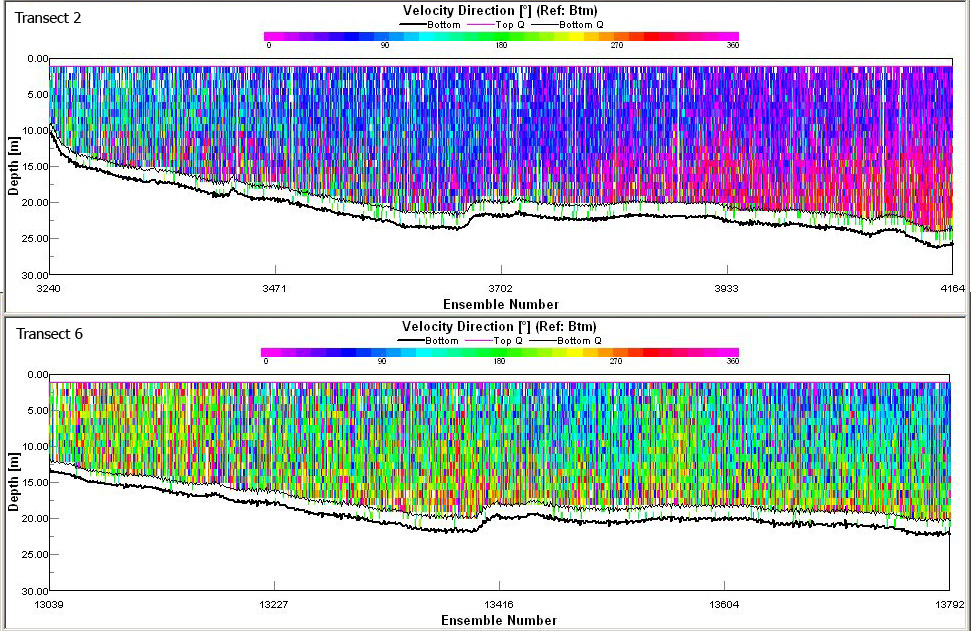
Fig 1.40 Direction 2 and 6 Transect 2 was taken at 09.45 – 10.05 GMT, approximately at high tide (09.46 GMT). Transect 6 was taken at 13.19 – 13.35 GMT, approximately 3.5hrs after high tide. It is interesting to see how the directional velocity has changed through the tide. Surface layers have stayed relatively constant, staying in an easterly/southerly direction. This may be the fresh water riverine discharge from both the Fal estuary and the River Helford. The lower surface waters have completely changed direction. At high water, bottom water net flow was in a northerly direction. As the tide ebbed, the direction swung around almost 180 degrees, and the mean net transport was in a southerly direction. The directional velocity become noisier and less uniform, suggesting that eddying may be occurring as the tide ebbs.
|
Fig 1.41 Direction 3 and 7 Transect 3 was taken at 10.18 – 10.42 GMT, approximately 45 minutes after high tide (09.46 GMT). Transect 7 was taken at 13.48 – 14.11 GMT, approximately 4hrs, after high tide. There is a change is direction in surface water, moving swinging from a northerly direction 45 minutes after high tide, to a south-easterly direction 4hrs after high tide. Deeper water also varies with tidal state, swinging from a north-westerly direction 45 minutes after high tide, to a south-westerly direction 4hrs after high tide. This again displays a basic clear two layer water column structure, depending on density.
|
 |
 |
|
Fig 1.42 Direction 4 and 8 Transect 4 was taken at 11.50 – 12.08, approximately 2hrs after high tide (09.46 GMT). Transect 8 was taken at 14.30 – 14.41, approximately 4.5hrs after high tide. Surface waters have changed from a north-easterly direction at 11.50 to a south easterly direction and 14.30. This change in surface water flow direction is due to the ebbing flow of both the Helford River and the Fal Estuary. Bottom waters have stayed relatively constant, with a constant, west/south-west direction.
|
Fig 1.43 Direction 5 and 9 Transect 5 was taken 12.37 – 12.53, approximately 3hrs after high tide (09.46 GMT). Transect 9 was taken at 14.52 – 15.05, approximately 5hrs after high tide. The northern end of both transects is highly influenced by the outflow of water from the Fal estuary. At both states of the tide, the movement of water was in a southerly direction. This means than in this regions, tidal currents dominates the directions of currents in the bay. The southern end of transect 5 (mid-tide), shows that the directional currents flow in an easterly direction. As the tide approaches low tide (transect 9), the region is dominated by a southerly flowing current. This means that the currents in Falmouth bay are most influenced by the Fal estuary’s ebbing water at low tide.
|
 |
 |
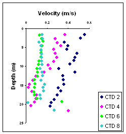 |
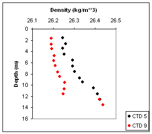
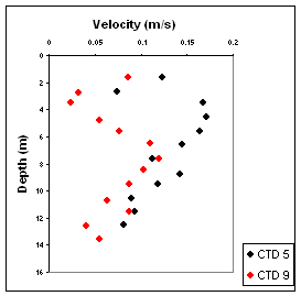
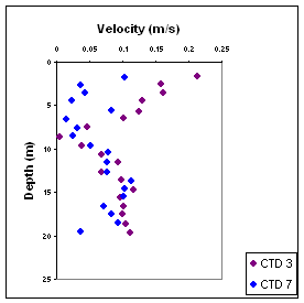
| Fig 1.7 Shows density profiles at CTD stations 5 and 9 taken at 1256 and 1508 GMT, respectively. | Fig 1.8 Shows velocity profiles at CTD stations 5 and 9. | Fig 1.9 Shows velocity profiles at CTD stations 2, 4, 6 and 8. taken at 1008, 1213, 1337 and 1444 GMT, respectively. |
 |
 |
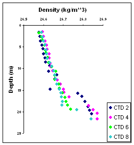 |
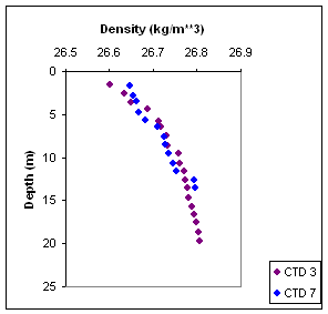
| Fig 1.10 Shows density profiles at CTD stations 3 and 7 taken at 1121 and 1413 GMT, respectively. | Fig 1.11 Shows density profiles at CTD stations 3 and 7. | Fig 1.12 Shows density profiles at CTD stations 2, 4, 6 and 8. |
Analysis of the Richardson number values showed variation in layer stability at most stations. An area of particular interest is the location of CTD casts 2, 4, 6 and 8. Many stable layers were found at CTD positions 6 and 8 whereas CTD positions 2 and 4 showed significantly fewer stable layers. Plots of density and velocity profiles show a relatively constant relationship with density and depth between stations at intimate locations, however, velocity is shown to have decreased throughout the survey between high and low water shown by the variation between stations at similar geographical locations. This would explain the increase in stable layers at CTD stations 6 and 8 as they were sampled at the later part of the survey at 1337 and 1444 GMT, respectively. This is unusual however as it is this period at mid-tide when you would expect maximum flow rates. Maximum flow rates were seen at stations 2 (time 1008 GMT) and 4 (time 1213 GMT) measuring 0.577 m/s and 0.369 m/s, respectively, explaining the low Ri numbers found there.
Discussion
Deployment of CTD 1 was performed during the flood tide at Black Rock (Station 1). Data from this station displayed a slight thermocline and halocline. Data obtained from CTD 5 and 9 during an ebb tide showed a well mixed water column, illustrating the influence of the ebb tide upon the mixing of the water column.
There were similar numbers of phytoplankton cells at each of the above CTD stations. As the samples were taken in close proximity cell numbers would not be expected to differ greatly over a tidal period. However, these numbers are much higher than those at more southerly stations (e.g. CTD 7). Station 1 is situated at the mouth of the Fal estuary, the higher cell numbers found at Station 1 could be due to higher nutrients being flushed from the Fal. Although CTD 7 is located close to the Helford River, it does not lie directly on the mouth as does Station 1 to the Fal and thus it is not guaranteed to receive the same level of nutrients.
Higher chlorophyll concentrations were noticed at Station 1 than at Station 3. This reflects the higher phytoplankton levels at Station 1. Lower zooplankton levels were seen at Station 1. This could also explain the high phytoplankton levels as they are not being grazed at a high rate. Higher numbers of zooplankton individuals at Station 3, may explain the low levels of phytoplankton and chlorophyll, indicating a higher grazing rate. Low oxygen saturation levels at Station 3 may limit photosynthesis, contributing to low abundance in phytoplankton.
The middle station (Station 2) showed homogenous properties at all four CTD sites suggesting that this is a well mixed water column. High chlorophyll concentrations were seen at CTD 4. However, as the only water sample taken at Station 2 was at CTD 4, it would be incorrect to draw conclusions about the plankton community interactions. Unfortunately, due to Niskin bottles failing to fire at all desired depths there is a lack of nutrient data for Station 2. High chlorophyll concentrations at CTD 4 could possibly be due to relatively high oxygen saturation (average 92.2%).
A time series of ADCP transects has shown variations in current magnitude and velocity throughout the tidal cycle. Transects were taken from high water (09.46GMT) until almost low water (16.04GT). The Falmouth Bay tidal currents are complicated by the addition of the River Helford riverine discharge. Two transects found increased levels of backscatter at mid-depths (~15m). This indicates the presence of zooplankton populations grazing on potential phytoplankton blooms. The directional velocity of net flow of bottom water changed almost 180 degrees over half a tidal cycle; high tide to low tide. Potential eddying occurred as the tide dropped, indicated by irregular contour plots for later transects. A two layer structure is visible when comparing the directional velocity contour plots, with deeper water flowing in the opposite direction to surface water. This induces shearing at the interface between the two. By combining this knowledge and applying Richardson number calculations to determine the stability, a deeper understanding of the physical nature of Falmouth Bay can be achieved.
~ Back to top ~
General Information
| Date: | 05/07/2008 |
 |
| Vessel: | R.V. Bill Conway and Ocean Adventure RIB | |
| Skipper: | Nigel and Kevin | |
| Crew: | Bob | |
| Demonstrator: | Peter Statham | |
| Area surveyed: | River Fal | |
|
Equipment Used: Link to Specifications |
CTD | |
| ADCP | ||
| Plankton net & digital flow meter | ||
| Anemometer |
| General Weather Notes | Cloud cover | Wind | Pressure (mb) | Temperature (oC) | ||
| Direction | Speed (ms-1) | Air | Sea Surface | |||
| Strong winds all day, total rainfall approx. 16ml | 8/8 | SW | 10 (gusting 15) | 1005 | 16.0 | 15.2 |
Aim
The aim of the survey was to see how the distribution of nutrients and plankton communities within the estuary are influenced by the vertical structure of the temperature, salinity and current velocities throughout the estuary, including the tributaries.
Survey method
Bill Conway Survey
Due to the unfavorable weather conditions RV Bill Conway started sampling at the mouth of the Fal River.
Surface water samples were collected periodically up the river against an ebbing tide.
Two plankton trawls were conducted on at the mouth of the Fal River and one near the confluence of the Truro and Fal Rivers.
5 ADCP transects and 4 vertical CTD profiles were conducted, with positions shown in figures 1 and 2. When the CTD was deployed the weather conditions and a secchi depth were also recorded.
Vertical profiles of Salinity and temperature, and water samples at set depths were collected using a rosette with YSI probe and 6x 1.7L Niskin bottles attached.
A sub sample was taken from each niskin bottle from which dissolved oxygen samples were taken and processed for storage using the Winkler method. The oxygen samples were then stored in full, glass Stoppard bottles submerged under water to stop addition of oxygen post collection. Replicate oxygen samples were collected this allowing for an indication of accuracy.
A second sub sample was taken from the niskin bottle; 60ml was filtered through a glass fiber filter with the last 50ml of the filtrate being collected in a rinsed plastic bottle. This plastic bottle was then stored in a cool box and the water sample was later analyzed in the laboratory for its silicon content.
A Final 60ml was then filtered through another glass fiber filter; again the last 50ml was collected and stored in a rinsed glass bottle with the water sample later analyzed in the laboratory for its nitrate and phosphate content.
Both of the used filters were then placed in separate containers with 6ml of 90% acetone solution for chlorophyll measurements in the laboratory.
| RIB Survey Method |
Click images to enlarge |
|
|
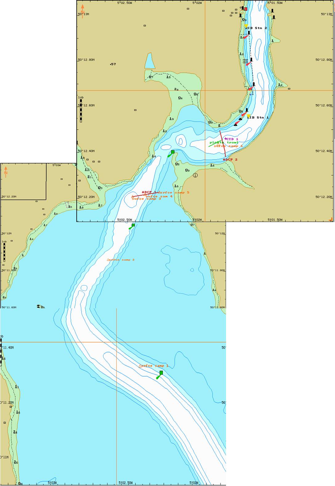 Fig 2.1 South section of area surveyed |
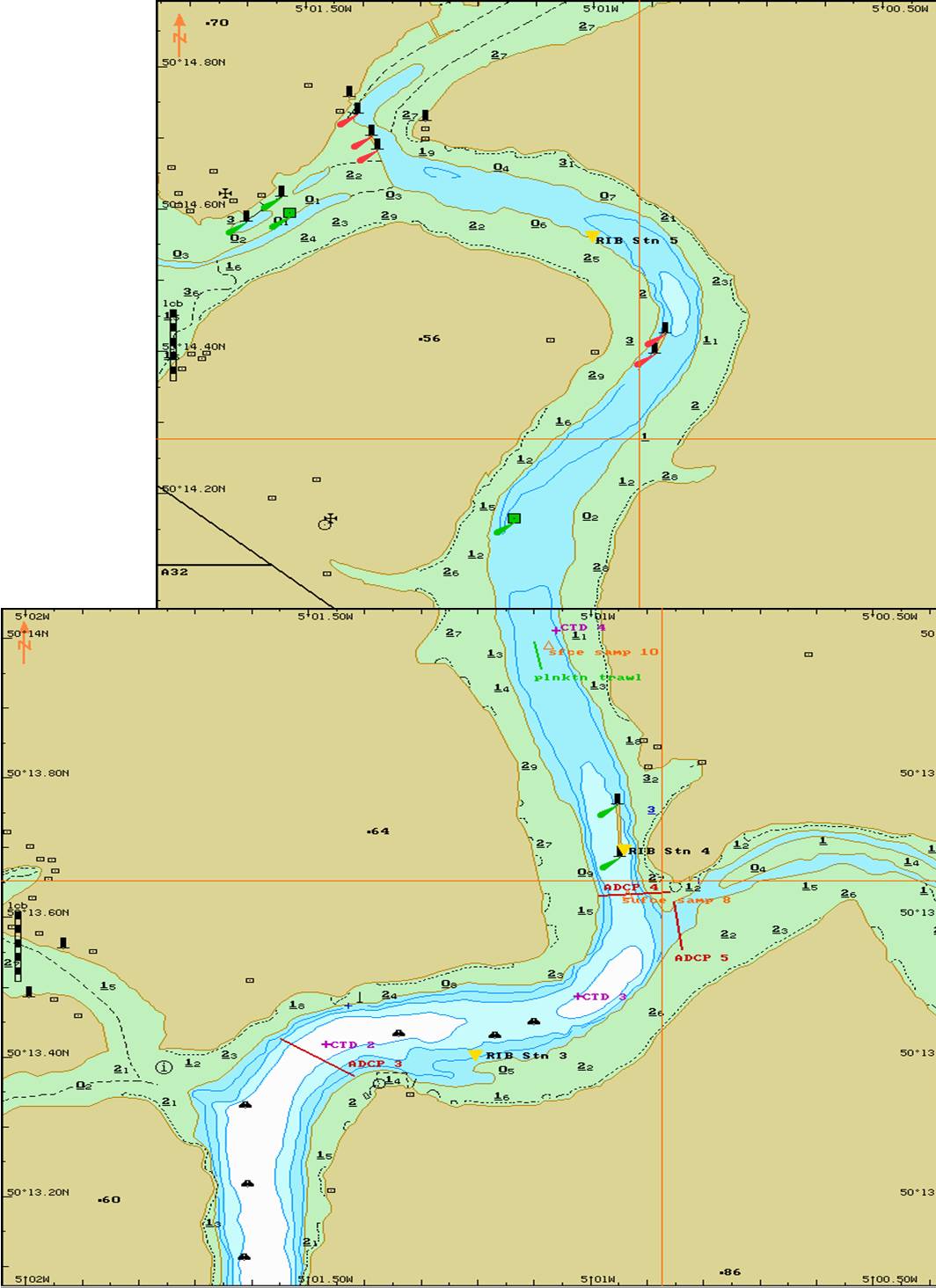 Fig 2.2 North section of area surveyed |
Calibration method
Due to use of different temperature and salinity probes (T/S probes) all salinities had to be calibrated. Firstly the Ocean Adventure temperatures and salinities had to be standardised to the Bill Conway temperatures and salinities. This was performed by deploying all the T/S probes of the Ocean Adventure and the Bill Conway in the same water at the same time to the same depth. The temperatures and salinities were recorded. Secondly vertical profiles of two T/S probes upon the Callista were made in order to obtain the appropriate equation. This equation was then used to calibrate the Ocean Adventure and Bill Conway temperatures and salinities to the Callista temperatures and salinities.
Chemical procedures and analysis
The water samples were analysed in a laboratory for the chlorophyll, dissolved Phosphate and Silicon concentrations using the method described by Parsons et al (1984). Dissolved oxygen was calculated following the Winkler method described by Grasshoff et al (1999). Nitrate concentrations were measured by Flow injection analysis as described by Johnson and Petty (1983).
Phytoplankton analysis: 100ml of solution in the lugol iodine glass bottles were left to settle. The top 90ml were then removed using a pump concentrating the sample to 10ml. 1ml of this sample was put into a gridded Sedgewick Rafter counting cell and studied under a microscope.
Zooplankton analysis: A sample was inserted into a Bogorov chamber and studied under a microscope.
Results and Discussion
Nutrients and CTD vertical profiles
Click on the thumbnails or hyperlinks to enlarge the graphs
|
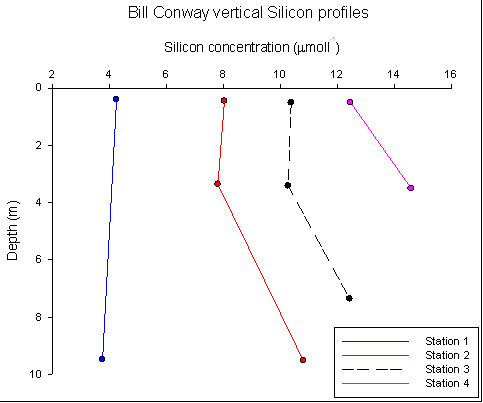
Silicon Silicon concentrations at Conway CTD Site 1 appear uniform with depth most likely due to the strong mixing at the mouth of the Fal, caused by the combination of large waves and spring tides which would produce a well mixed water column. Conway CTD sites 2 and 3 show similar profiles. It is likely that due to limited geographical separation, any hydrodynamic or ecological processes in operation will act similarly. Conway CTD site 4 appears to show an increase of silicon with depth however this could be due to poor resolution as only two sample depths were taken. |
Fig 2.3 Silicon vertical profile |
|
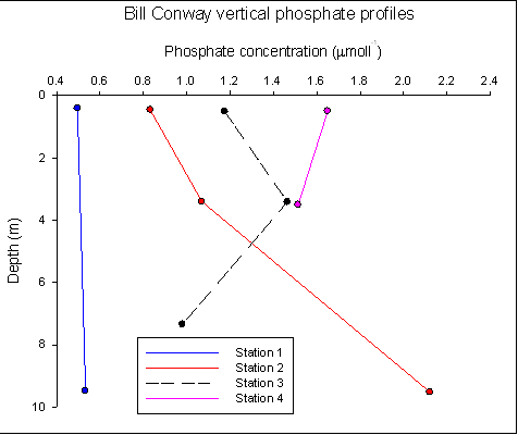
Phosphate Conway CTD site 1 is again homogeneous likely due to mixing at the entrance of the river. Above 4m, Conway CTD 2 and 3 show similar profiles. The large value for the 10m sample in site 2 (>21 µmol l-1) is likely to be anomalous; a decrease similar to site 3 would be expected considering owing to their close proximity. |
Fig 2.4 Phosphate vertical profile |
|
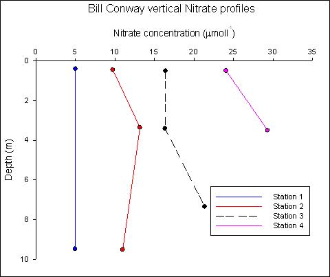
Nitrate Conway CTD Station 1 appears to be homogeneous; however owing to the paucity of data between to the surface and 10m samples interpretation is limited. Taking into account the unfavourable conditions (ref), the apparent changes observed in sites 2 and 3 may be due to sampling error. Conway Site 4 shows levels of nitrate much greater than all other sites at a surface concentration of 24µgl-1. However, RIB site 4 reported a dramatic decrease in nitrate concentrations between Conway sites 3 and 4, which owing to their close proximity it is likely to be a sampling error. |
Fig 2.5 Nitrate vertical profile |
|
Salinity and Temperature Profiles are homogeneous at all stations indicating a well mixed water column most likely caused by the high winds. |
|
|
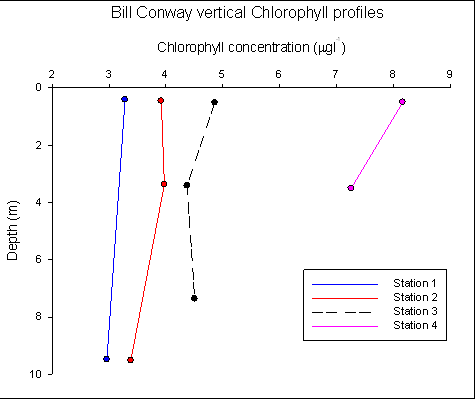
Chlorophyll Conway CTD Sites 1, 2 and 3 located in the Fal River appear uniform with depth, however station 4 exhibits a decrease in chlorophyll concentration with depth. RIB station 5 reported the highest surface chlorophyll concentration (>9µgl-1) of all the sample sites, which is likely due to its location in the Truro River which reported the highest measured nutrient concentrations. |
Fig 2.6 Chlorophyll vertical profile |
|
Dissolved O2 The oxygen depth profile shows a general decrease in oxygen with depth. This is expected because the biggest source of oxygen is diffused from the atmosphere at the water-air interface. RIB station 5 shows the lowest oxygen content as well as the sharpest drop in oxygen content. This is a relatively shallow, close to shore area and the decrease in oxygen may be due to plant matter in the water decomposing. |
Fig 2.7 Dissolved O2 vertical profile |
|
Richardson Number Analysis of the density profiles in the water column calculated using calibrated salinity, temperature and depth readings taken from the YSI probe onboard the Bill Conway showed intense vertical turbulence and overturning. Therefore meaning any Richardson number calculations are invalid. |
|

|
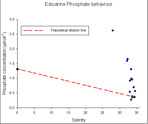
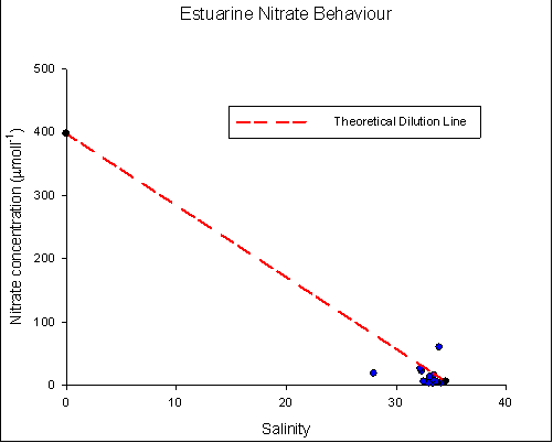
Phosphate: Strongly non-conservative behaviour evident from data collected. [PO43-] at Rib station 5 is over 4 times that which is expected from the TDL. (REF) Whilst continuous addition exists through weathering of rocks, the large fluxes evident in this region are likely be attributed to domestic (washing powders), agricultural (fertiliser runoff). This may explain the high count of 32000 cells l-1 at RIB station 5. (see Phytoplankton table of results). |
Fig 2.8 Phosphate vs. salinity |
|
Nitrate: Photoautotrophic utilisation by macro and microphytes present in abundance are likely due to the high levels of phosphate. Nitrate also being a plant nutrient is likely to be depleted in this situation due to the increased intake caused by the rapid phytoplankton population growth. |
Fig 2.9 Nitrate vs. saliinty |
|
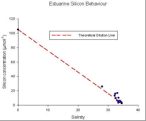
Silicon: Remineralisation of diatoms (forming the previous spring bloom event in this part of the estuary) possibly explains the addition of this nutrient to the lower reaches and hence the non-conservative behaviour observed. Since no known external fluxes exist in this area, liberation solely from the water column is probable. |
Fig 2.10 Phosphate vs. salinity |
Phytoplankton and Zooplankton
The phytoplankton samples collected on the RIB and Bill Conway have much higher total number of diatoms than dinoflagellates, with 128 000 cells per litre and 45 000 cells per litre respectively. This is as expected because diatoms are more able to tolerate mixed conditions, which were experienced on the day of sampling. Dinoflagellates thrive more in stratified waters. It is also easier to identify diatoms as they are generally larger. The samples from the RIB do not appear to show any pattern in the number of diatoms or dinoflagellates at each station as we move up the river. This is most likely due the fact that samples were being taken in storm conditions when large amount of mixing would have been taking place.
Phytoplankton table of results
 |
 |
| Fig 2.11 Pie chart showing contribution of main Diatom groups | Fig 2.12 Pie chart showing contribution of main Dinoflagellate groups |
Due to the high winds on the day of data collection only two plankton net trawls were carried out. Trawl A was conducted near the mouth of the Truro river (050o12.427 005o01.910). Trawl B was conducted further south in the Fal river (050o12.992 005o01.063).
A reason for the differences between the zooplankton population composition at the two different trawls sites is likely to be due to changes in environmental conditions between the sites. For example there is a relative increase in Cirripedia larvae in sample A and reduced Gastropoda larvae populations compared to sample B. A reason for this change could be due to changes in the salinity or nutrient concentration. The salinity at trawl B (30.7) is reduced compared with trawl A (34.1) and the nutrient concentrations are higher at trawl B. Cirripedia can be thought of as being Stenohaline were as some Gastropods are Eurohaline and can therefore reproduce in lower salinitys. This leads to there geographical separations as the Gastropods are able to survive and reproduce higher in the estuary therefore leading to there increase in numbers.
An additional factor which could affect zooplankton abundance is the abundance of phytoplankton (prey) at each location. Phytoplankton population are larger at trawl B (which is likely to be linked to the increased nutrient concentrations) than A which could explain why zooplankton are more numerous at site B.
 |
 |
| Fig 2.13 Pie chart showing the composition of zooplankton groups from net trawl A. | Fig 2.14 Pie chart showing the composition of zooplankton groups from net trawl B. |
| Dominant Phytoplankton Identified | Dominant Zooplankton Identified |
| Dinoflagellates: Alexandrium and Dinophysis | Sample A: Copepods, Copepoda nauplii and Cirripedia larvae |
| Diatoms: Chaetoceros, Rhizosolenia | Sample B: Copepods, Copepoda nauplii and Gastropod larvae. |
Table 2.1 Names of dominant phytoplankton and zooplankton found in our samples. Click on the hyperlinks to view photos taken through the microscopes of particular phytoplankton types.
ADCP data and profiles
Transect 1 - ADCP contour plot is not complete enough to produce any reliable data. Significant wave height due exposure to a force 8 southerly wind caused ADCP to break the surface of the water, resulting in blanks sections in the contour plot. For this reason, transects 2, 3, 4 and 5 will be analysed instead.
| Velocity Direction contour plots | Velocity magnitude contour plots | Average backscatter contour plots |
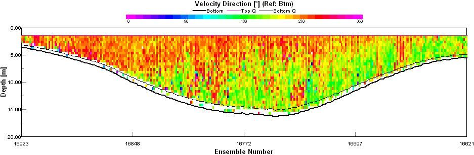
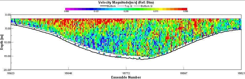
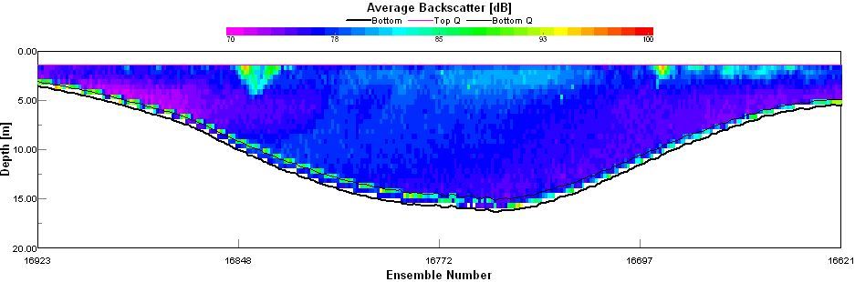
| Transect 2 - Length of transect: 200m Start: 50° 12.495N, 005° 01.831W End: 50° 12.384N, 005° 01.797W | ||
 |
 |
 |
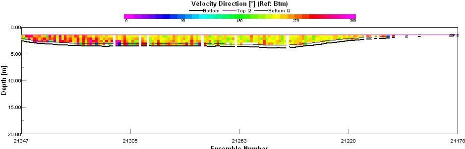
| Fig 2.15 The directional contour plot shows the net flow of water at transect 2 was in a WSW direction. The north end of the transect has a net flow in a westerly direction and the south end of the transect has a net flow in a south-westerly direction. The transect was taken at 09.07GMT, and low water was at 13.21GMT, hence, the tide was ebbing. The direction of flow fits with the direction of flow due to the tide. |
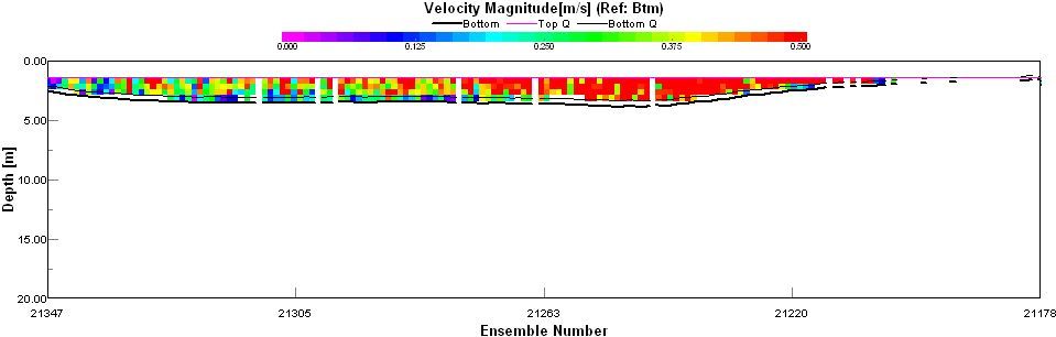
Fig 2.16 The velocity magnitude of the flow at transect 2 varies across the transect. The south end of the transect, on the outside of the bend in the river, is ~0.25 m/s faster than north end of the transect, on the inside of the bend in the river. This variation in velocity is due to helical flow. |
Fig 2.17 Backscatter indicates the amount of activity throughout the transect. Regions of increased backscatter occur in the surface waters, 0m to ~1.5m depth. This may be due to wind-induced waves breaking at surface, causing turbidity. Bottom waters also produce increased backscatter caused by suspended sediments, due to frictional currents flowing along the seabed. |
| Transect 3 - Length of transect: 193m Start: 50° 13.429N, 005° 01.547W End: 50° 13.376N, 005° 01.417W | ||
 |
 |
 |
| Fig 2.18 The directional contour plot shows the net flow of water at transect 3 was in a W-SW direction. The north end of the transect has a net flow in a south westerly direction and the south end of the transect has a net flow in a westerly direction. The transect was taken at 10.18GMT, and low water was at 13.21GMT, hence, the tide was ebbing. The direction of flow fits with the direction of flow due to the tide. |
Fig 2.19 The velocity magnitude of the flow at transect 3 varies across the transect. The north end of the transect, on inside of the bend in the river, is ~0.20 m/s slower than south end of the transect, on the outside of the bend in the river. This variation in velocity is due to helical flow |
Fig 2.20 There are two prominent regions of backscatter near the surface that stand out from the rest of the transect. One maximum at 2m depth at the north end of transect and a second maximum at 4.5m depth. This may indicate a increased chlorophyll levels due to a phytoplankton bloom. |
| Transect 4 - Length of transect: 119m Start: 50° 13.632N, 005° 00.984W End: 50° 13.639N, 005° 00.860W | ||
 |
 |
 |
|
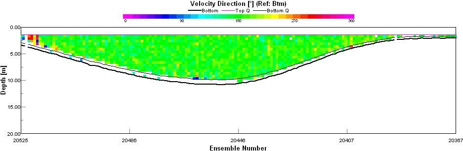
Fig 2.21 The directional contour plot shows the net flow of water at transect 4 was in a southerly direction across the mouth of the Truro River tributary. The direction of the net flow was homogonous throughout the transect and water column. Very little variation occurred, due to a very intense ebb flow. The transect was taken at 10.45GMT, and low water was at 13.21GMT. |
Fig 2.22 The velocity magnitude of the flow at transect 4 varies across the transect. The magnitude of the flow is higher in the centre of the channel (~4m/s), where frictional influences by the sea bed are minimal. Flow at the edge of the channel is slower (~2.5m/s). |
Fig 2.23 The most prominent region of backscatter is located at ensemble number 20411 and at a depth of ~2m. This indicates increased levels of chlorophyll and a potential phytoplankton bloom. |
|
Transect 5 - Length of transect: 126m Start: 50° 13.623N, 005° 00.855W End: 50° 13.557N, 005° 00.840W |
||
 |
 |
 |
|
Fig 2.24 Transect 5 was across the mouth of a very shallow section in the River Fal. The south end of the transect clearly shows a westerly net flow and the north end of the transect shows south westerly net flow. |
Fig 2.25 The north end of transect 5 has a high magnitude of net flow (~5m/s). The south end of the transect shows a reduced magnitude in flow velocity. This may be due to shallower waters and increased friction with the seabed. |
Fig 2.26 The middle of the transect shows a patch of increased backscatter. Due to the shallow depth of the water, this could be a region of suspended sediment of a phytoplankton bloom. CTD samples will need to be used to clarify the what is causing this increase in backscatter. |
~ Back to top ~
General Information
| Date: | 02/07/2008 |
 |
| Vessel: | Xplorer | |
| Skipper: | Robin | |
| Crew: | Steve | |
| Demonstrator: | John Davis | |
| Area surveyed: | Fal Estuary - North of Bay | |
| Equipment Used: | Sidescan sonar | |
| Van Veen Grab | ||
| Video Camera | ||
| Digital Camera |
| General Weather Notes | Cloud cover | Wind | Pressure (mb) | Temperature (oC) | ||
| Direction | Speed (knots) | Air | Sea Surface | |||
| Light breeze with a short period of light rain | 4/8-7/8 | WSW | 13-18 | 1008 (steady) | 19.8 | 14.3 |
Aim
To investigate and classify sea bed type using geophysical acoustic techniques and use the data calibrated with grab samples and video footage to infer flora and fauna, physical water properties and geology.
Factors affecting transect selection
Selection of a transect location was restricted by prevailing weather conditions and survey time in relation to tidal period. Strong winds producing waves in excess of 2 metres produces a highly distorted image due to undulations in tow fish position relative to the sea floor. This led to the decision to perform the survey in the more sheltered estuarine environment.
Beginning the survey in the morning of 2nd
July 2008 meant navigation of the estuary on the flood tide from low water of
1.1m at 1045 GMT. The result is the transect location needed to be where lowest
astronomical tide was in excess of 1m allowing for safe passage of the boat
(1.5m draft) and tow fish. Analysis of Natural England data showed Areas of
Conservation ideal for analysis due to varying physical and biological
properties. West Falmouth Bank lying in the South of Mylor Pool and North of
Falmouth Harbour has previously been found to have areas of eelgrass and
rocky/sandy sediment. This position relative to the shore is likely to produce
variation in current flow from interfacial and bottom friction meaning a likely
variation of sediment types and features away from the shore. The
characteristics of this location makes it an ideal candidate for the conduction
of a side scan sonar survey and is likely to produce a sonagraph with complex
tonal properties, a range of sea bed features and hopefully a variety of
physical and biological components for analysis.
allowing for safe passage of the boat
(1.5m draft) and tow fish. Analysis of Natural England data showed Areas of
Conservation ideal for analysis due to varying physical and biological
properties. West Falmouth Bank lying in the South of Mylor Pool and North of
Falmouth Harbour has previously been found to have areas of eelgrass and
rocky/sandy sediment. This position relative to the shore is likely to produce
variation in current flow from interfacial and bottom friction meaning a likely
variation of sediment types and features away from the shore. The
characteristics of this location makes it an ideal candidate for the conduction
of a side scan sonar survey and is likely to produce a sonagraph with complex
tonal properties, a range of sea bed features and hopefully a variety of
physical and biological components for analysis.
Transect location and time details
Method
The Xplorer surveyed along 3 transect lines 100 m apart at 4.5-5knots with a towfish attached to the starboard corner, deployed just beneath the water surface.
The trace was studied and potential grab sites recorded at areas of interest.
These locations were returned to on completion of the survey, with one grab sample per transect line.
Using the onboard winch, a van veen grab was deployed to collect seabed surface samples. the contents were sieved and analysed on board.
Images of the seabed were obtained using a video camera attached to a static line.
Traces from the sonograph were analysed and features were measured through trigonometric caluculations.
Results
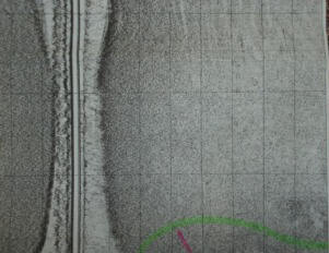
Sonagraph trace
The sediment is predominantly fine material, mainly mud and silt. Various bedforms were identified, such as ripples, rock protrusions and depressions (See Sonagraph images below).
Click on the following trace thumbnails to enlarge.
 |
 |
 |
|
Fig 3.2 Homogenous fine sediment at position 50o10.6340N, 005o02.178W |
Fig 3.3Depression in sediment (1.37m) at position (50o10.6340N, 005o02.5893W). The depression is likely to be a relic of the underlying geomorphology and not a function of any impact upon the seabed. |
Fig 3.4 Bedrock protrusion in an area of coarse sediment at position 50o10.383N, 005o02.180W |
 |
 |
 |
|
Fig 3.5 Location of grab 1 at position 50°09.9107N, 005°02.6096W. |
Fig 3.6 Location of grab 2 at position 50°09.6420N, 005°02.9374W . Shows ripples measuring 0.238m in height and 2.22m in wavelength. They can be seen to be wave induced as indicated by the bifurcation. |
Fig 3.7 Location of grab 3 at position 50°10.1510N, 005°02.6383W. Showing protrusion of bedrock surrounded by gritty mud with high content of biogenic material, including dead maerl. |
Grab results
There was a distinct difference between all three grabs obtained during this survey. Sediment consisted mainly of mud and some biogenic material. The grab samples were taken in areas that were not within the central deep channel of the estuary. This was around 20m deep and the shallower areas were around 6m deep. In these shallower areas there were suitable light levels to observe the actual seabed using a video camera. This confirmed our initial expectations of the features of the seabed. Grab 3 had coarser sediment due to high amounts of dead maerl. Living biota decreased from grab 1 to grab 3, possibly due to the increase in dead calcareous algae which can be seen as an indication of high disturbance.
| Grab no. | Fullness and general description | Classification | Further classification |
 Increase in dead maerl |
 Increase in anoxic properties |
| 1 | 10% fullness of grab | Rhodophyta | Callophyliis laciniata, Palmaria palmata | ||
| Mud and clay | Mollusca: Gastropoda | Family Trochidae | |||
| High amounts of biogenic material | Crustacea | ||||
| Ascidia | |||||
| Annelida: Polychaeta | |||||
| 2 | 20% fullness of grab | Rhodophyta | Ceramium rubrum | ||
| Mud and clay | Mollusca: Gastropoda | ||||
| 3 | 40% fullness of grab | Maerl | |||
| Coarse grain | Mollusca | Trivia monacha |
Table 3. Biotic and abiotic details of grab samples.
Discussion
|
Monitoring
of the sonagraph print out allowed for decision of the location for grab samples
in areas of interest. Figure 1
shows Grab 3, originally intended to sample what we thought to be eelgrass but
this area was over shot. The tone shown can be interpreted to be coarse grain
via grab
sample calibration. Figure 2 shows an intrusion of the underlying
geology into the overlying coarse sediment. Figure 3 shows fine sediment in an
area of deep water (9metres). The image however
has been darkened due to poor
photograph replication. Figure 4 shows the site of Grab 1 where fine mud and
clay were found in the grab sample. Figure 5 shows a depression measuring 1.37m
likely to be a function of the underlying geomorphology. Sub surface profile
using instrumentation such as a boomer is necessary to determine the bed rock
affect. Figure 6 shows ripples measuring 0.238m high and are clearly wave
induced as indicated by bifurcation. This is common in shallow waters such as
this. It is probable that a fair weather wave base is modulating the feature
shown. Assessment of the historical ‘wave climate’ is required to validate this
assumption. It is important to note that when analysing a sonagraph print out, if certain assumptions, as described by Blondel and Murton (1997) are not met then the trace may show artefacts and distortions which can lead to the appearance of apparent features which do not represent any solid physical feature on the seabed. One of the assumption is that the seabed underneath the fish is horizontal with no mean gradient over the swath width. Our data is collected from a transect near the west bank of the Fal estuary so has a slopping seabed which could have lead to distortion of our data. Three grabs are not enough to represent the flora and fauna which inhabit the area. In order to obtain a more accurate picture, many more samples would have to be taken and species would have to be counted and identified in more detail. |
click to enlarge
|
~ Back to top ~
During our two weeks in Falmouth we achieved our objective of analyzing the physico-chemical and biological properties of the Fal Estuary. The weather experienced during our stay was a major hindrance and we found that our desired survey plans could rarely be conducted fully. The results have shown the Fal Estuary to be fully mixed, however it is difficult to separate our finding from long term process whereby mixing due to stormy conditions may have masked any processes that would have been detected in calmer conditions. We were unable to penetrate far up river but found that there is a deep inland salt water penetration limit and unfortunately were unable to survey offshore but could see the influence of the estuary within the offshore survey areas. There are clear nutrient gradients from the river environment to the offshore, as expected, with high signals of phosphate within the river.
The data set obtained is not representative of the whole area and was too small to draw any accurate conclusions about the different aspects of the Fal Estuary. The sample size was not large enough to allow for any anomalous results. The data contained in this website provides a temporal snapshot of certain features and should not be viewed in isolation as representative of the full area. Diurnal, monthly, annual and inter-annual variations between data sets exist for a number of reasons and as such, analysis is tentative.
~ Back to top ~
Bishop, G.M. and Holme, N.A. Nature Conservancy Council. CSD Report (1980)
Blondel, P and Murton, B.J. (1997) Handbook of seafloor sonar imagery. Wiley, Chichester. p.314
Grasshoff, K.., Kremling, K., and M. Ehrhardt. (1999). Methods of seawater analysis. 3rd ed.
Wiley-VCH.
Johnson K. and Petty R.L.(1983) Determination of nitrate and nitrite in seawater by flow injection analysis. Limnology and Oceanography. 28: 1260-1266.
Mullin and Riley (1955) Analytica Chimica Acta. 12: 162
Parsons, T. R., Maita Y. and Lalli C. (1984) A manual of chemical and biological methods for seawater analysis. 173 p. Pergamon.
~ Back to top ~