|
|
|
|
|
|
Click images for larger versions
![]()
![]()
![]()
![]()
![]()
![]()
![]()
|
|
|
|
|
|
![]()
![]()
![]()
![]()
![]()
![]()
![]()

.jpg)
Aims
To understand how vertical mixing processes directly and indirectly affect the structure and functional properties of plankton communities.
Logistics
Date: 02/07/2008
Location: Offshore
Time: 0800-1330 GMT
Tide: LW 1045, 1.1m
HW 1627, 5.2m
Range 4.3m, Spring tide
Conditions: SE winds 5-6, Sea State- Moderate,
Cloud cover 5/8
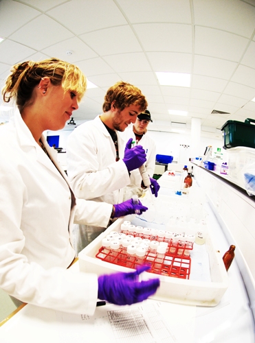
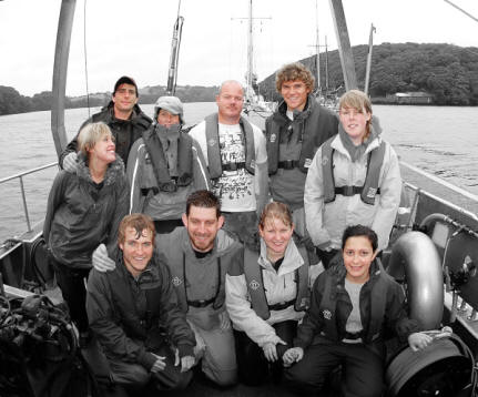
The Team
PSO: Scotty
Scribe: Alex B
Stern Deck team: Bill, Alex S, Ed
Wet lab team: Natalia, Annabelle, Jess
Dry lab team: Mat, Hannah
![]()
![]()
![]()
The Fal Estuary is situated in Cornwall on the South coast of England, (Fig. 1.0). It has six major tributaries, including Helford River, Restronguet Creek and Carnon River, and 28 smaller creeks. The estuary is defined by type as a Ria, a river valley drowned as a consequence of the end of the last glacial maximum. The Fal Estuary is the third largest natural harbour by volume in the world. The deepest section of the estuary is known as the Carrick Roads and is 34m deep at chart datum. Carrick Roads is fed by the Fal River, Penrhyn River and Percuil River.
The mean tidal range of the Fal Estuary in Springs is 4.6m and in Neaps is 2.2m; this means that the tides are macro-tidal during Springs and meso-tidal during Neaps. The weather of the Fal region is dominated by Westerly Maritime airflows during the summer months; causing relatively high precipitation and therefore high run off. This high run off facilitates the high flux of nutrients into the estuary due to the proximity of agricultural regions to the Fal.
The Fal is the most metal polluted estuary in England, caused by mining, sewage discharge, agriculture and Tri-Butyl Tin. Past mining activity has resulted in elevated quantities of trace metals in both the water column and sediments. The Wheal Jane incident in 1992 caused major spikes in metal concentrations, especially copper and zinc, when the pumps were stopped and the mine flooded (Langston et al. 2003).
The main aims of this field course are to measure the chemical, physical and biological structure of the estuary and offshore. This will allow a comparison of both regions during the summer months.
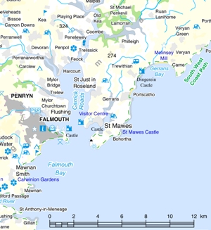
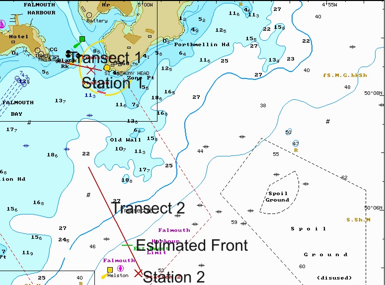
Figure 1.0 - An Overview of the study area
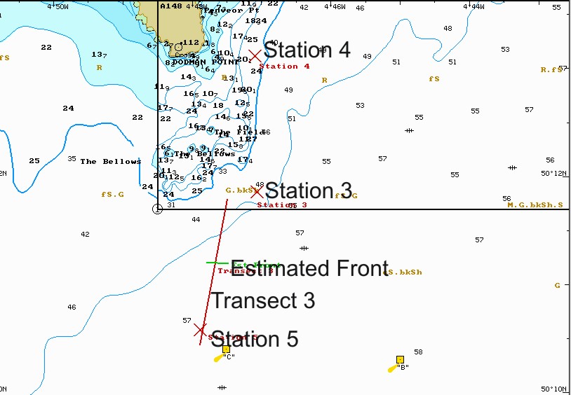
Sampling began at Black Rock at 0840, station 1. A transect across the mouth of the estuary from Shag Rock to Black Rock was conducted and the ADCP was set to record during this time. Following this, a transect southwards was carried out to find the shelf sea tidal front. This was located 3 miles south of Black Rock and station 2 was set up on the stratified seaward side. Travelling east toward Dodman Point and sampling occurred at station 3, just inshore of the tidal front. Station 4 was located inshore and a transect, with ADCP recording, was performed to 2 ½ miles south of Dodman Point where a final station, station 5, was sampled.

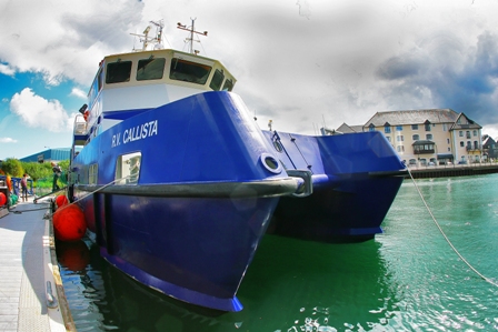
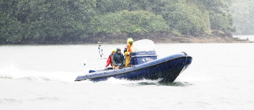
The RV Callista – Offshore Research
|
Vessel Dimensions |
Deck |
Scientific Equipment |
|
Length - 19.75m
Draft - 1.80m Max Speed - 15 knots Range – 400 nautical miles |
‘A’ Frame and associated winch – 4 tonne lifting capacity 2 x over the side davits of 100kg Capstan 1.5 tonne pull |
ADCP CTD and rosette Digital thermosalinograph Fluorometer Transmissometer Secchi disc Closing zooplankton net
|
|
Vessel Dimensions |
Deck |
Scientific Equipment |
|
Length - 11.74m Beam - 3.96 Draft: - 1.3m Max speed - 10 knots Cruising Speed - 9 knots, Range - 150 nautical miles |
A-Frame: Stern – 750kg, 3m max height Davits x 2 Port and Starboard – 50kg, 15m wire length Trawl Winch: Max wire length 70m (8mm) Capstan: 0.25 Tonne |
ADCP CTD Digital thermosalinograph Secchi disk Towed zooplankton net
|
|
Vessel Dimensions |
Deck |
Scientific Equipment |
|
Length - 7.00m
Beam - 2.55m
Draft - 0.5m
Max Speed -
35 knots Cruising Speed - 25 knots, Range - 100 nautical miles |
All over the side work to be done by hand |
YSI Probe Temperature-Salinity probe (TS probe) Secchi Disc Phytoplankton Net and Zooplankton Net
|
|
Vessel Dimensions |
Deck |
Scientific Equipment |
|
Length – 12m Beam – 5.2m Draft – 1.2m Max Speed – 25 knots Cruising Speed – 18 knots |
Deck crane with winch Hydraulic capstan – 1 tonne |
Side scan sonar Van Veen Grabs
|
Niskin Bottles
Niskin Bottles are used to obtain in situ water samples from different depths in the water column. These samples can then be analysed for pH, chemical constituents and chlorophyll.
Glass Fibre Filters
Glass Fibre Filters are used to filter the nutrient samples to remove plankton. The filter papers can then be used for chlorophyll analysis, by acetone extraction.
Hydroline, with Messenger, and Depth Sensor
The Niskin Bottle is attached to a Hydroline and a Messenger is sent down the line to trigger the closing mechanism when the Niskin bottle is at the required depth. The depth is recorded on a Depth Sensor, which is attached to the Niskin bottle.
Zooplankton Net (200μm)
A 200μm Plankton Net is used to obtain a concentrated sample of zooplankton. The 200μm net mesh catches mainly zooplankton cells to be quantified and identified.
Van Veen Grab
The Van Veen Grab is used to obtain a sediment sample, which can be analysed to determine the physical, chemical and biological processes occurring at the sediment-water interface.
Secchi Disc
A Secchi Disc is used to determine the light penetration into the water column. Three times the depth at which the Secchi Disc can no longer be seen by the human eye is a rough indication of the lower level of the euphotic zone. The Secchi depth can also be used to calculation the light attenuation coefficient. The Secchi depth may vary depending on the eyesight of the user, therefore consistency is preferable.
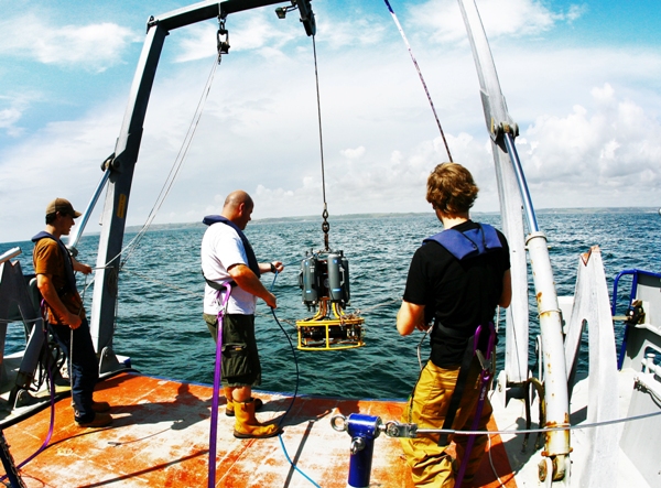
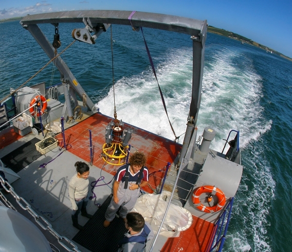
CTD Rosette
The CTD is used to measure conductivity and temperature, with depth. Conductivity can be used as a proxy for salinity. It is lowered through the water column to produce a profile. The CTD is mounted on a rosette allowing easy attachment of other equipment, such as Niskin bottles, a Fluorometer and a Transmissometer.
ADCP
The ADCP (Acoustic Doppler Current Profiler) is used to measure the speed and direction of currents in the water, using an acoustic Doppler technique. The backscatter intensity gives an indication of both particulate matter and plankton, within the water column.
YSI Multiprobe
The YSI Multiprobe is used to measure temperature, dissolved oxygen concentration, chlorophyll concentration, salinity and pH, with depth.
T/S Probe
A T/S Probe is used to measure temperature and salinity, through the water column. These two parameters are manually recorded to produce a temperature and salinity profile, with depth.
Side Scan Sonar
Side Scan Sonar is used to produce an image of the sea floor by emitting sonar pulses and producing a backscatter image. A transducer emits pulses, which spread over a distance of about 150 metres, and the returning pulses are plotted against travel-time to produce an image. The transducer is pulled along on a tow fish, although it can be mounted on to the vessel, in order to eliminate any external sounds affecting the data. Different frequencies can be emitted: higher frequencies improve the resolution of the images, however the range is reduced.
|
|
|||
|
|
|||
Nutrient Analysis
Nitrate analysis method
Nitrate analysis followed the flow injection analysis, as described by Johnson and Petty (1983), with a detection limit of 0.1µM. The results were produced on a chart recorder.
Phosphate analysis method
Phosphate analysis method, similar to that used to measure silicate, was outlined by Parsons et al. (1984). The Hitachi spectrophotometer was used to analyse the samples and standards added to the manual 4cm cell. The sample absorbencies were analysed relative to the absorbencies gained from the known laboratory standards. The detection limit for phosphate was 0.03µM.
Silicate analysis method
Silicate concentration was measured using the method, outlined by Parsons et al. (1984), with a detection limit of 0.3µM. The Hitachi spectrophotometer was used to compose a calibration curve of absorbance against known standard silicate concentrations prepared in the laboratory. The equation of the line was then used to determine the unknown concentrations of silicate in the samples from their absorbance values.
Dissolved oxygen analysis method
1ml of two Winkler reagents were added to the seawater samples on the vessel and kept cool for laboratory analysis. The dissolved oxygen content was calculated using the method outlined in Grasshoff et al. (1999).
Biological Analysis
Chlorophyll analysis method
Glass fibre filters used on board the vessel were put into 6ml of acetone to extract the chlorophyll. The samples were refrigerated over night. In the laboratory, the filter papers were removed and the remaining liquid was analysed using a Turner fluorometer. The fluorescence reading was then converted to give the chlorophyll extract of the original sample.
Phytoplankton taxonomy analysis method
1ml of Lugols iodine was added to 100ml of seawater sample on board the vessel and allowed to settle. The water was then decanted and the concentrated phytoplankton solution was analysed under a low power microscope and counted in Rafter cells.
Zooplankton taxonomy analysis method
10 ml of formalin was added to the 500ml samples gained from the closing plankton net after transference to the plastic bottles. After mixing, a 5ml aliquot was observed for taxonomic and quantitative analysis under low power microscopes in a Bogorov tray. The numbers were multiplied up to gain estimations on the numbers present in the cylindrical column of water through which the net was hauled.
Dissolved Silicon results
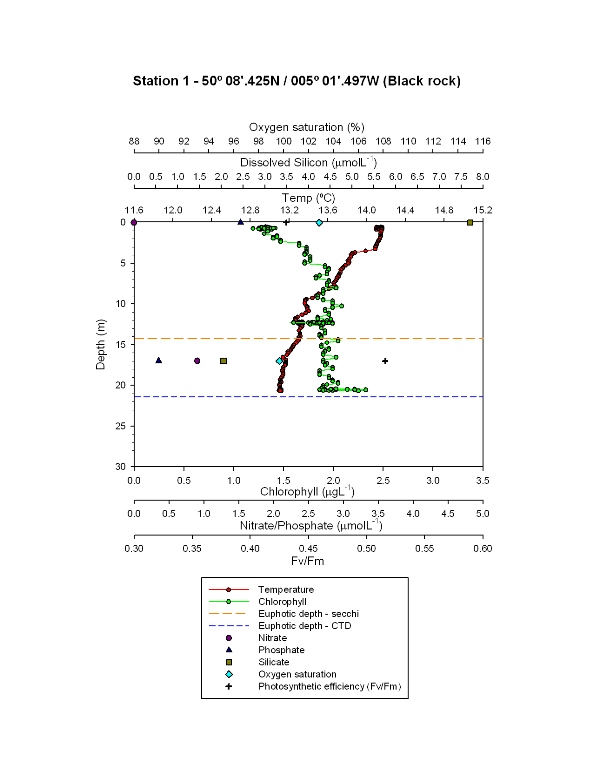
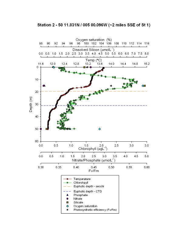
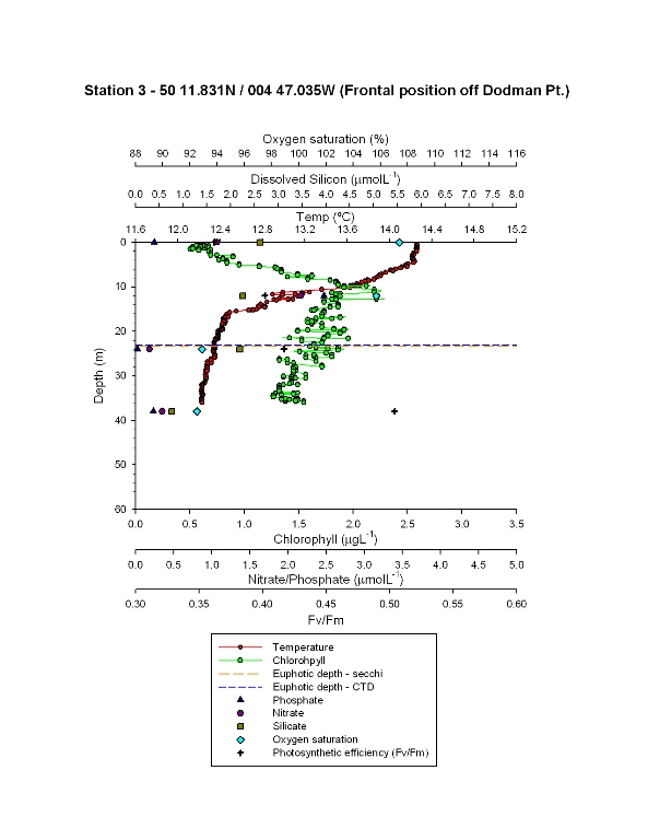
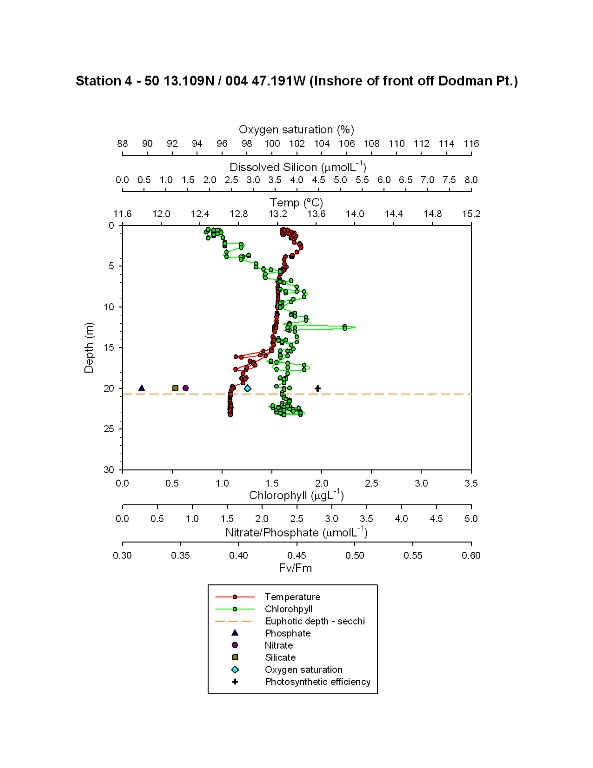
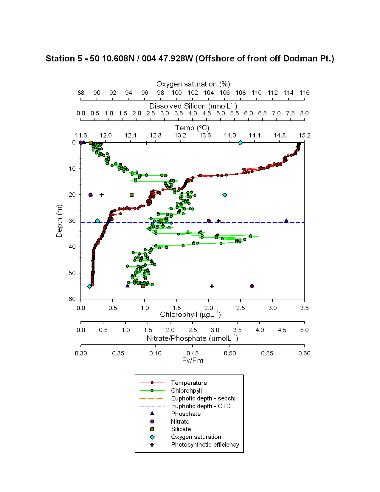
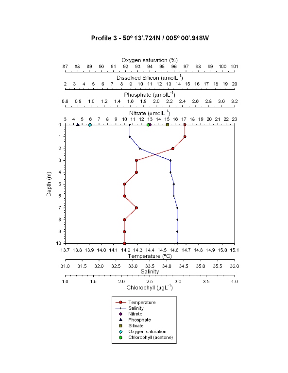
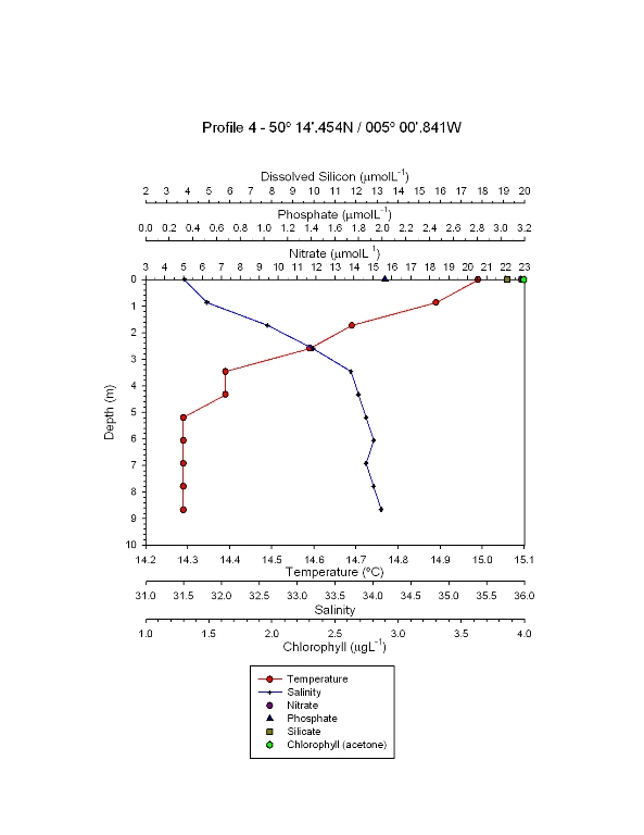
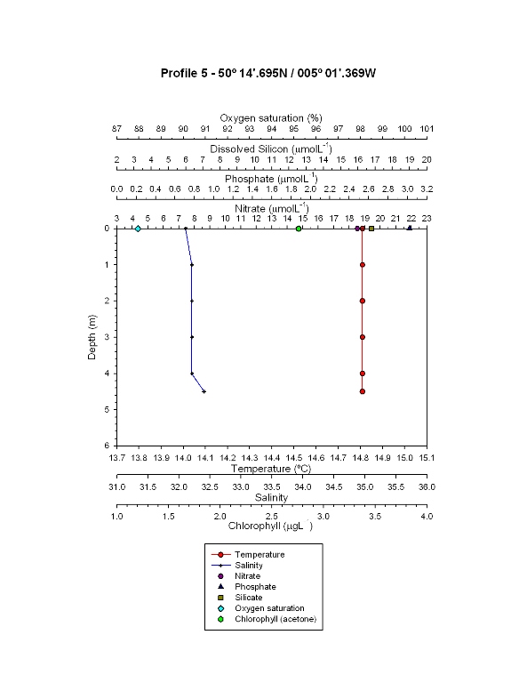
Silicon at Station 1 (Fig 4.06) decreases from a concentration of 7.71µmol L-1 at the surface, to a concentration of 2.05µmol L-1 at 17m depth. Station 2 (Fig 4.07) shows an increase in silicon concentration from the surface to 15m depth by 4.54µmol L-1. At 50m the concentration had decreased to 0.4373µmol L-1. At Station 3 (Fig 4.08) there is a steady decrease in the surface waters from a concentration of 2.62µmol L-1 at the surface to 2.19µmol L-1 at a depth of 24m. From 24m to 38m there is a rapid decrease to 0.77µmol L-1. Only one sample was taken at station 4 (Fig 4.09), at 20m depth, and a concentration of 1.22µmol L-1 was recorded. The final station, Station 5 (Fig 4.10), shows a steady increase in concentration from the surface to a depth of 30m, from 0.36µmol L-1 to 2.88µmol L-1. After 30m depth there is a decrease in concentration, up to 55m depth, of 2.24µmol L-1.
Phosphate
The phosphate concentration decreases from 0-17m by 0.07µmol L-1 m-1 at station 1 (Fig 4.06). Station 2 (Fig 4.07) shows a decrease in nitrate from the surface down to the thermocline, beneath which it increases by a rate of 0.035µmol L-1 m-1. Phosphate at Station 3 (Fig 4.08) is low at the surface increasing by 2.23µmol L-1 until 12m depth, phosphate then decreases to a minimum concentration of 0.03µmol L‑1 at 24m. At 38m depth, phosphate concentrations return to that of the surface. Around 19m, all the stations, including the one data point for station 4 (Fig 4.09), show similar low phosphate concentrations. Station 5 (Fig 4.10) shows the greatest variation in phosphate. There is a small increase in concentration in the top 20m followed by a rapid increase of 4.4µmol L-1 over 10m then a rapid decrease of 3.6µmol L-1 over the final 15m.
|
|
|||
|
|
|||
At each station samples were taken in the following way. A CTD down-cast was recorded and Niskin bottles were fired at appropriate depths. Water samples were collected from the Niskin bottles;
a sample for dissolved oxygen was taken before any other contamination could occur and was fixed using Winkler reagents,
100ml was stored for phytoplankton analysis,
60ml was filtered through glass fibre filter and sorted in glass bottles for nitrate and phosphate analysis,
60ml was filtered through a pre-flushed glass fibre filter and stored in plastic bottles for silicate analysis.
The filters used in the preparation of the nutrients samples were placed into acetone to extract the chlorophyll. A 200µm mesh plankton net was deployed and lowered to a known depth. The water samples had formalin added to them to preserve the plankton caught. The euphotic depth was measured using a Secchi disk and the cloud cover was noted.
Nitrate
A consistent increase in nitrate is shown from 0-17m at station 1 (Fig 4.06). Station 4 (Fig 4.09) shows a similar nitrate concentration as stations 1 and 3 at the similar depth. Station 3 (Fig 4.08) has 1.1µmol L-1 at the surface then increases down to 11.6m then a rapid decrease down to 24.1m where, like station 2 (Fig 4.07) after 14.6m, nitrate remains fairly constant. Station 2 exhibits the greatest concentration of nitrate in seawater, with 2.3µmol L-1 at the surface which then decreases rapidly to 0.1µmol L-1 at 14.6m. Station 5 (Fig 4.10) shows a dramatically different trend of increasing nitrate with depth from the negligible amount of nitrate present at the surface. The greatest increase was at a rate of 0.3µmol L-1 m-1 between 20.2m and 29.8m.
Dissolved Oxygen
Dissolved oxygen is higher at the surface and decreases rapidly at the thermocline at all stations except station 2 (Fig 4.07). Station 1 (Fig 4.06) is well mixed which is reflected by the marginal but consistent decrease in dissolved oxygen with depth. Both stations 3 and 5 (Figs 4.08 and 4.10) show a rapid decrease in dissolved oxygen with depth to the thermocline from 107.5% to 92% and 90% saturation respectively. Station 4 (Fig 4.09) only has one point but shows a similar level of oxygen saturation at 20m to Station 1. The curve from station 2 shows an increase from 91.4% at the surface to 115% at the thermocline (15m deep) and then shows a steady decrease with depth.
|
|
|
|
|
Station 4 - Fig 4.09
This site shows the smallest change in temperature with depth, being 13.2 ºC at surface and 12.7 ºC at 23m depth. The chlorophyll maxima was found to be at 12.4m with chlorophyll levels of 2.2 µgL-1. Only the Secchi disc was used to estimate the euphotic depth at 20.7m.
Station 5 - Fig 4.10
Station 5 showed the greatest thermal variation in the water column, from 15.1 ºC at the surface to 12.1 ºC at 26m and decreasing to a minimum of 11.7 ºC at 54m depth.
The chlorophyll maximum was positioned below the thermocline at 36m, with values of 2.7 µgL-1, also showing a secondary peak of 1.8 µgL-1 at 20m. Photosynthetic efficiency was highest at the base of the euphotic zone (estimated at 30m using the Secchi disc and 30.6m using the CTD) and remains high at the maximum sampling depth (55m).
Zooplankton
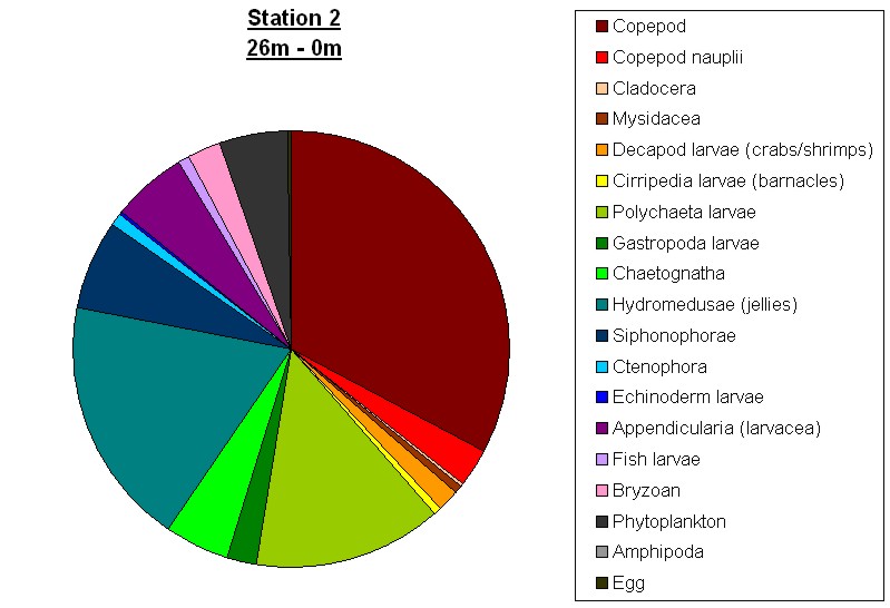
The two catches at Station 2 result a direct comparison of the organisms present in the top 20m and that in the top 26m. The deeper catch produced a smaller proportion of copepods, gastropod larvae and siphonophores, but a larger catch of polychaete larvae, hydromedusae and other less abundant taxonomic groups.
|
|
|
|
|
|
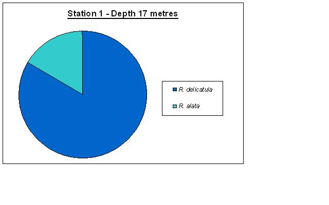
Phytoplankton
At Station 1, illustrated in Fig. 4.16 and Fig. 4.17, a diatom species was found to be the most abundant (83% of the total cells identified) along with one dinoflagellate species. At 17m depth two species of diatoms were present but no dinoflagellates.
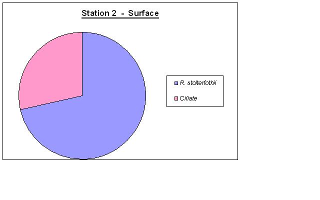
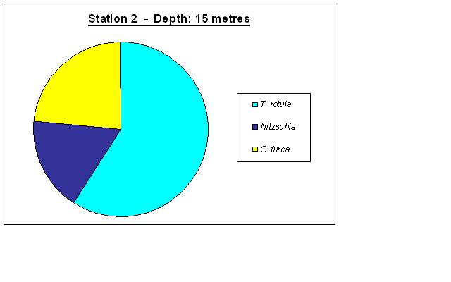
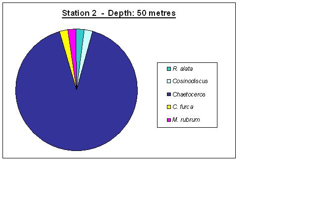
At the surface of Station 2, shown in Fig. 4.18, the diatoms species Rhizosolenia stolterfothii (71%) and ciliate species silicate (29%) were present. Fig. 4.19 shows that at 15m water depth two diatom species were identified and one dinoflagellate species. At 50m there were three diatom species making up 95% of the species identified, depicted in Fig. 4.20, and also one ciliate and one dinoflagellate species present.
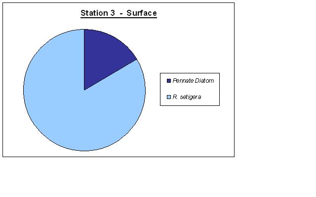
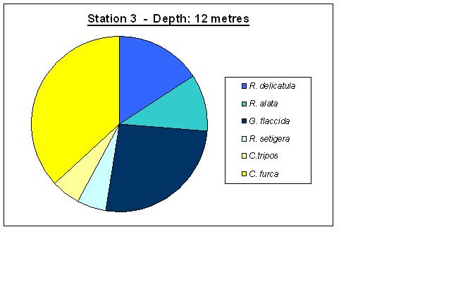
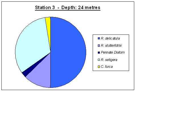
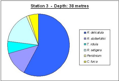
At Station 3, represented in Fig. 4.21, Fig. 4.22, Fig. 4.23 and Fig. 4.24, only pennate diatoms were found such as Rhizosolenia setigera. 12m from the surface, diatoms dominated but the dinoflagellates Ceratium tripos and Ceratium furca were present. At 24m 98% of the species identified were diatoms. From the deepest sample, at 38m; 4 diatom species were identified composing 94% of the population.
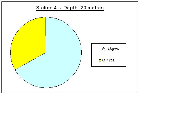
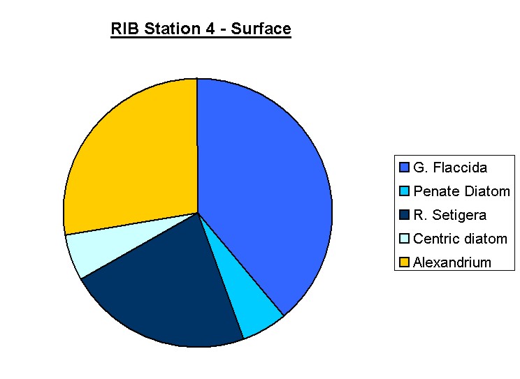
From the 20m depth sample at Station 4, Fig. 4.25, R. setigera made up 67% of the population and the dinoflagellate C. furca the remaining 33%.
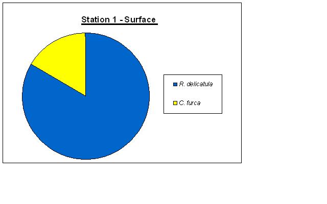
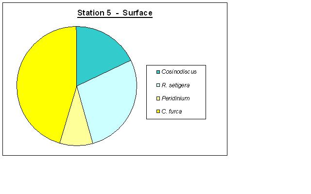
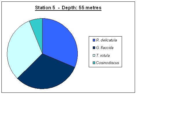
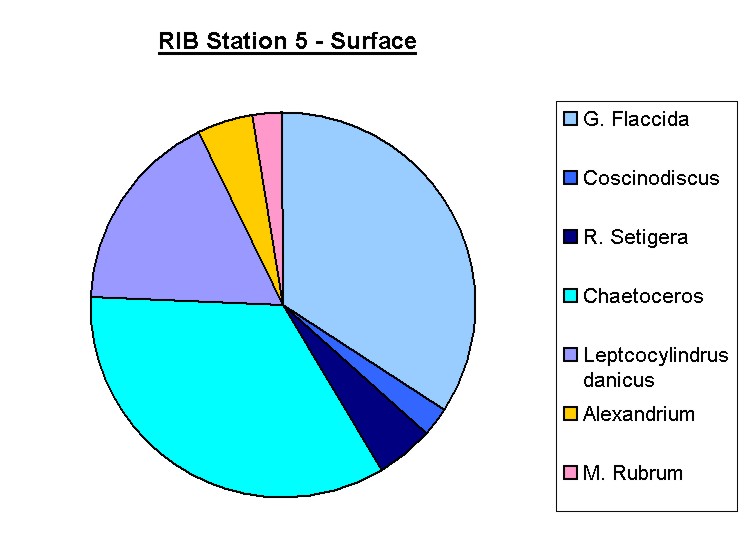
On the surface of stratified side of the tidal front (Station 5), dinoflagellate species were found to dominate, portrayed in Fig. 4.26. Two species of dinoflagellates were identified; C. furca (83%) and Peridinium (17%) along with two species of diatoms. At 20m depth, Fig. 4.27, 3 diatom species were identified (74% of the total cells of this sample) and one dinoflagellate species (36%). At 30m depth, 7 diatom species were identified including Rhizosolenia delicatula, the most dominant contributing 56% of the total diatom species, Fig. 4.28. At 55m depth, four diatom species were identified, shown in Fig. 4.29: R.delicata, Guinardia flaccida and Thalassiosira rotula were all found in equal proportions of 31% each; in addition Cosinodiscus was identified.
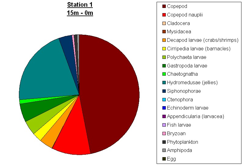
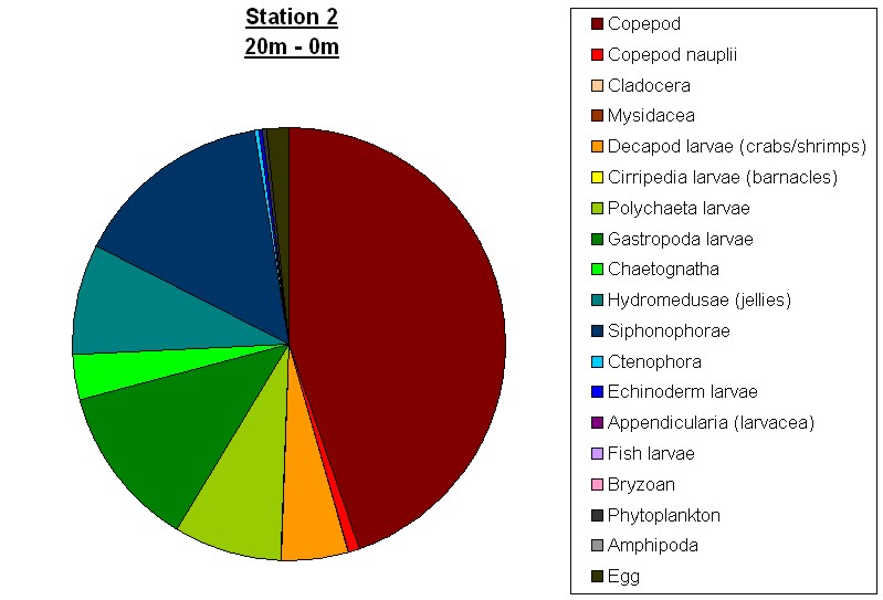
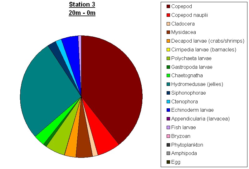
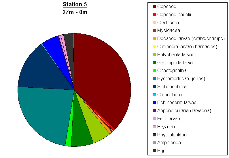
At all stations, as shown in (Fig. 4.11, Fig 4.12, Fig 4.13, Fig 4.14 and Fig 4.15), copepods dominate, varying from a 33% to 47% proportion. Hydromedusae occupy the next greatest proportion and, with the siphonophores, make up to 37% of the samples. 17 different categories of zooplankton were found along with one category for eggs and one general category for visible phytoplankton. These categories range encompassing 13 individuals per m3, e.g. Mysidacea in the water column at station 5, to 2829 per m3, e.g. copepods also at station 5
The samples from the top 20m of water at Station 2 and Station 3 shown in pie charts (Fig 4.12, Fig 4.13 and Fig 4.14), show great variations especially in proportion of Hydromedusa and Siphonophores, differences of 19% and 13% respectively. Station 2 was recorded to have a lower diversity, 4 less groups observed, but has fewer groups with low abundances.
Similarly two stations, 2 and 5, sampling occurred over the top 27m, their results show a large similarity with only great differences in the abundance of polychaete larvae and siphonophores and the presence of ctenophores, echinoderm larvae and appendicularia.
|
|
|
|
|
|
|
|
|
|
|
|
|
|
|
![]() Physical
Physical
ADCP Transect Results
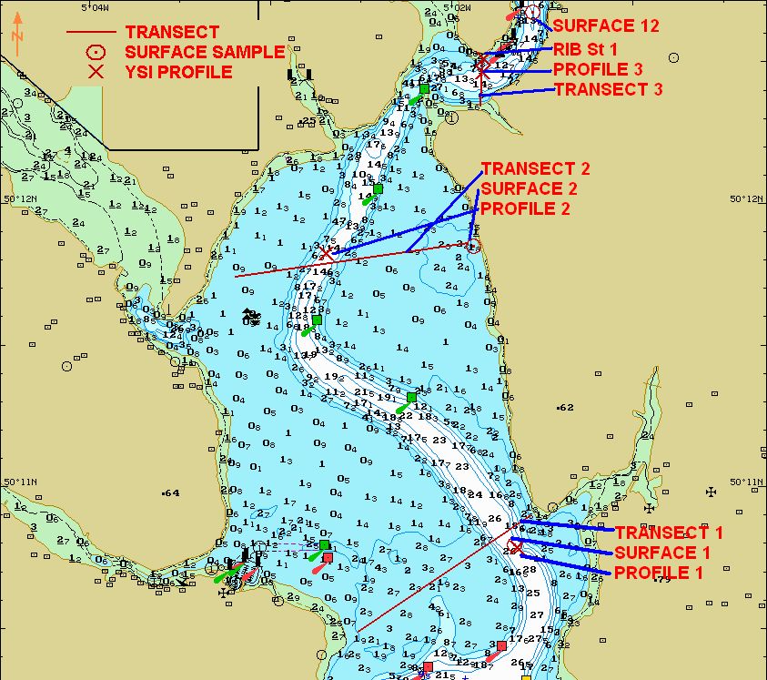
Transects 2 and 3 both crossed the tidal mixing front. The frontal positions are shown on Fig 4.01 and Fig 4.02, and are given below:
Transect 2 Front at 50 º 05.1’N 005 º 00.3’W
Transect 3 Front at 50º 11.2’N 004º 47.7’W
Figs 4.03 and 4.04 show ADCP backscatter intensity due to Zooplankton grazing activity, and give an image of the fronts and thermocline.
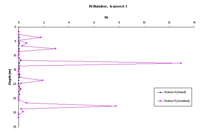
For transect 3 , stations 4 and 5 are at the inshore and offshore sides of the front, and this has allowed the Richardson (Ri) number to be calculated , giving stability profiles inshore and offshore. The plot of Ri numbers, Fig 4.05 shows a well mixed water column at station 4, and the CTD profile at station 4 (Fig 4.09) shows little vertical structure. A clear stability maximum (Ri 12.95) at 12.6m is shown at station 5, which corresponds closely with the thermocline observed in the CTD profile at depth of 12m. Station 3 appears to be somewhat thermally stratified, which suggests it is close offshore of the front. No ADCP data was available at the station. Comparing the known position of the front on transect 3, with the position of station 3 located 0.75 Nautical Miles (NM) to the NNE, it would seem probable that the front is approximately following the 50m depth contour.
|
|
Transect 2 |
Transect 3 |
||
|
|
Inshore |
Offshore |
Inshore |
Offshore |
|
Depth (m) |
Unavailable |
55 |
20 |
57.00 |
|
Estimated Thermocline depth from ADCP (m) |
N/A |
15 |
N/A |
12.60 |
|
Estimated Thermocline depth from CTD (m) |
N/A |
16 |
N/A |
12 |
It is interesting to note that the CTD and Ri number profiles at station 5 show a second thermal stratification, below the main thermocline, at a depth of 26m. A fluorescence maximum was also observed below the main thermocline, at 35m, however there does not appear to be any physical structure associated with this feature.
Table 4.0 summarizes the main features of the front and thermocline at each transect. It can be seen that the bathymetry at which stratification can occur is similar in each case. This suggests that the thermal and tidal energy inputs are similar at both locations, which would be expected because they are only 11NM apart. The difference in thermocline depth between the two transects may be due to an internal wave in the thermocline.
|
|
|
|
|
|
CTD Results
Station 1 - Fig 4.06
A decrease in temperature from 14.1ºC at the surface to 13.1ºC at 20m was found at station 1. There was a chlorophyll maximum located at 20m depth with concentrations of 2.3µgL-1. Photosynthetic efficiency increases with depth from 0.43 at the surface to 0.52 at 17m sample. The Secchi depth was used to calculate a euphotic depth of 14.25m, which was found to be 7.15m shallower than the CTD calculated depth of euphotic zone which was 21.4m.
Station 2 - Fig 4.07
The temperature decreased from at the 13.7 ºC surface to 11.8 ºC at 50m depth .
Chlorophyll levels reach a maximum of 3.2 µgL-1 at 11.5m which is a four-fold increase compared to surface levels. The euphotic depth using the Secchi disc was calculated as 19.5m and from the CTD it was calculated at 31m deep. Photosynthetic efficiency was greatest at the chlorophyll maxima, and lowest at 50m, which was the maximum sampling depth. Oxygen saturation was greatest at the chlorophyll maxima at 115% and lowest at the surface (91%).
Station 3 - Fig 4.08
The temperature decreased from 14.3 ºC at the surface to 12.5 ºC at 15m. The chlorophyll maxima was located at the thermocline with concentrations of 2.2 µgL-1 which were almost four times the concentration at the surface (0.6 µgL-1). Photosynthetic efficiency gradually increases with depth, being greatest at 38m. The euphotic zone from the CTD was found to be 23.1m deep and using the Secchi disc was at 23.4m.
Stations 1 and 5 have the lowest surface nitrate levels. Station 1 also has the greatest levels of dissolved silicon at the surface. Corresponding to this, and due to the weak stratification which they prefer, diatoms dominate the phytoplankton community. Station 1 exhibits weak thermal stratification, due to greater tidal influence and mixing at the mouth of the estuary. It also has consistently high chlorophyll levels throughout the water column, which do not vary as much as other stations. High dissolved silicon is found at the surface, which decreases with depth as diatom abundance increases; as they utilise silicate to build their silica tests.
Station 5 has the strongest stratification and ADCP data has found a stable theromocline (Ri = 12.95). Dinoflagellates were the abundant phytoplankton group (>80%) at the surface, due to the increased stability at this site. Diatoms became more abundant with depth. Nitrate levels are lowest at the surface (nearly zero) and are highest of all the stations at depth. This could be explained by regeneration of nutrients below the thermocline (at 12m) and corresponds to a minimum in oxygen saturation, due to increased recycling. Dissolved silicon increases with depth at station 5, which may influence phytoplankton communities with depth, as more may lead to increased abundance of diatoms.
|
|
|||
|
||||
|
|
|||
Aim
The Aim was to conduct a survey the benthic habitat of the Fal Estuary. Due to the tide and inclement weather, the survey took place near-shore in the river Fal.
Logistics
Date: 05/07/2008
Location: River Fal
Time: 0845-1400 GMT
Tide: HW 0650, 5.1m
LW 1320 0.6m
Range 4.5m
Conditions: SE veering S winds, Cloud cover 8/8, drizzle to rain all day
Team
PSO: Annabelle
Scribe: Hannah
Navigation check: Ed, Mat
Grab sorting: Jess, Natalia, Alex B
Sidescan analysis: Scotty, Alex S
Video analysis: Bill
Photography: Alex B
Tea Boy: Mat
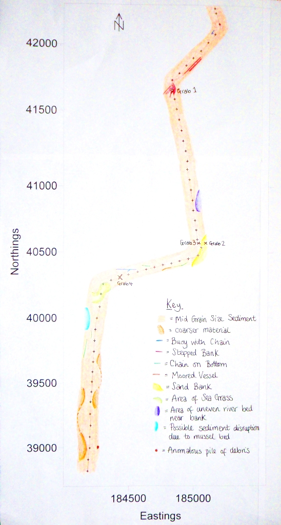
The survey consisted of a single transect between Turnaware Bar and Woodbury Point up the River Fal due to bad weather conditions preventing surveying in the estuary. The tow fish used 100kHz frequency and a total swath of 150m. As surveying took place up the river, the swath covered the entire channel, so only one transect was needed. The fish was deployed at 1000 UTC and recovered at 1050 UTC. Bottom grabs were taken at four separate locations based on observations from the sidescan plot. Location choices were based on changes in grain size and other features. Grabs were taken at Church Creek, Polgerran Wood and Lamouth Creek. Two grabs were taken at Polgerran Wood to compare areas of changing sediment bed type across the river. Once grabs were taken, they were analysed for sediment type, using sieves of 2mm and 1mm, and flora and fauna. Due to the bad weather and increased turbidity it was not possible to use the underwater video camera.
![]()
Sonograph
The backscatter shows that the river bed sediment throughout the length of the river is generally mid-grain size. There are areas of different sediment composition, as indicated by lighter or darker backscatter on the sonograph. Each turn is visible on the sonograph due to features that would normally be straight, being recorded as curves. Finally, there are some features recorded on the sonograph, such as buoys and chains, as well as the sediment structure.
Features recorded on the sonograph are listed in Table 5.0.
Grab 2 Edge of Polgerran Wood
Position: 50° 13.554 N
05° 00.920 W
Time: 11:43:02 GMT
Water Depth: 9.4m
Weather: Drizzle
Cloud cover: 8/8
Wind speed: 28 knots
Air temperature: 13.5ºC
Air pressure: 1004mb
Sediment
Grabs 2 and 3 were selected due to there being a possible sand bar present on the edge of the river. The two grabs were taken in order to discover the difference in sediment composition at the edge and centre of the river at this point. Grab 2 was positioned 15m to the east of the track plot at the sandbar. The sediment gathered from the grab at this site is coarse and pale in colour. The sediment is mainly composed of dead broken shell fragments and Maerl. There was a thin oxic layer at the surface of the mud and sand. The coarser nature of the sediment agrees with the idea of a sand bar present.
|
Fauna |
Number of alive individuals |
Number of dead individuals |
|
Netted Dogwhelk – Hinia neticulata |
1 |
0 |
|
Scallop – Chlamys vaia |
0 |
1 |
|
Clam (Mollusc, Bivalve) too small to identify |
2 |
0 |
|
Anemone (Cnidaria, Anthozoan) too small to identify, found as epifauna on scallop shell |
1 |
0 |
|
Bryozoan, too small to identify, found as epifauna on scallop shell |
present |
- |
|
Peacock Worm – Sabella pavonona |
2 |
0 |
|
Polychaete – Scoloplos armiger |
1 |
0 |
Table 5.2 - Fauna found in grab 2
Grab 1 Church Creek
Position: 50° 14.133N
05° 01.131W
Time: 11.07.18 GMT
Water depth: 3.3m
Weather: Raining
Cloud cover 8/8
Wind speed: 25 knots
Temperature: 13.2ºC
Pressure: 1003mb
Sediment
The position of the first grab was chosen due to possible sand bars seen on the track plot. This would suggest sediment of coarse grain and sandy in composition. The sediment sample collected in grab 1 was very dark and anoxic, which is expected up the river. The grain size of the sediment was fine mud, and there were fragments of Maerl present. This does not fully agree with the original hypothesis but this may be due to the drift of the boat whilst sampling.
|
Fauna |
Number of alive individuals |
Number of dead individuals |
|
Green Shore Crab - Carcinus maenas |
1 |
0 |
|
Barnacles – Acasta spongites |
Present |
- |
|
Slipper Limpets -Crepidula fornicata |
10 |
6 |
|
Oysters – Ostrea edulis |
3 |
7 |
|
Peacock Worms – Sabella pavonona |
11 |
3 |
|
Banded Carpet Shell – Paphia rhomboides |
1 |
1 |
|
Clam (Mollusc, Bivalve) too small to identify |
1 |
2 |
|
Scallop – Chlamys vaia |
0 |
1 |
| Time | Position on Sonograph | Feature | Bedform | Turn |
|
10:14:19– 10:17:49 |
West | - | Coarse Sediment | |
| 10:14:59– 10:15:08 | East | Anomalous Pile Of Debris | - | |
| 10:17:19– 10:20:49 | East | - | Coarse Sediment | |
| 10:20:31– 10:21:42 | West | Chain | - | |
| 10:21:45– 10:22:12 | West | Chain | - | |
| 10:22:19– 10:23:19 | West | - | Possible Sediment Disruption From Mussels | |
| 10:23:49– 10:25:22 | East and West | - | Sea Grass | West |
| 10:26:13– 10:27:31 | West | Buoy with Chain | - | |
| 10:47:32– 10:47:50 | West | Chain | - | |
| 10:29:28– 10:30:10 | East | Vessel | - | |
| 10:30:24– 10:31:33 | East | Chain | - | |
| 10:31:30– 10:33:30 | East | - | Sand Bar | North |
| 10:42:27– 10:45:58 | East and West | - | Stepped Bank | North East |
| 10:28:00– 10:28:42 | East | Buoy with Chain | - |
Table 5.1 - Fauna found in grab 1
Grab 4 Lamouth Creek
Position: 50° 13.339N
05° 01.402W
Time: 12:28:42 GMT (Van Veen grab misfire)
12:29:54 GMT
Water depth: 10.0m
Weather: Cloud cover: 8/8
Wind speed: 28 knots
Temperature: 13.7
Pressure: 1003mb
Sediment
The position of grab 4 was selected due to distortions on the track plot, thought to be sea grass. However no sea grass was found as sampling took place in the fish track and not above of the expected areas of sea grass. This is due to the drift of the boat. The sediment gathered was very anoxic mud/clay, black in colour with extremely shallow oxic layer due to highly reduced conditions in the sediment. Fine sediments with little bioclastic material were observed. This was the finest material sampled, which is expected as this is the station furthest down river, and therefore the slowest river flow.
|
Fauna |
Number of alive individuals |
Number of dead individuals |
|
Polychaete Worm - Malacoceros fuliginosus |
1 |
0 |
|
Banded Carpet Shell – Paphia rhomboides |
0 |
3 |
|
Cockle Shell – Cerastoderma edule |
0 |
1
|
| Table 5.4 - Fauna found in grab 4 | ||
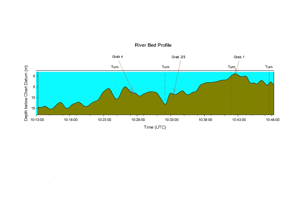
The river bed profile (Fig. 5.02) shows the depth of the river generally increases from the river’s head towards the river’s mouth. It does not increase at a steady rate due to sand bars and bends in the river. E.g. At the river bend after grabs 2 and 3, Lalmouth Creek and Cowlands Creek join the river Fal causing increased helical velocity and therefore increased water depth.
|
||||
![]()
Sonogram Analysis
Sediments are coarse upriver due to increased flow and are finer downriver as the river widens and flow velocity decreases. Grabs taken from upriver include coarser material than those taken from downriver. Being a sheltered river system, anoxic sediments are common, even near the mouth of the river. This is unexpected in most river systems, as anoxia generally increases further upstream.
Anoxia did increase upriver, with grab 1 being more anoxic than grabs 2 and 3, however, grab 4 was the most anoxic and was taken the furthest downriver. The sonogram suggests that the riverbed in the area around grab 4 is mainly composed of sea-grass, with this being comparable to studies undertaken by Foden et al. (2005), in the Fleet system where sea-grass has been found growing in anoxic sediments. Sea-grass is able to grow in anoxic sediments because they are able to extract oxygen directly from the water column through their subulate leaves (www.eoearth.org). However, the grab taken from site 4 contained no sea-grass due to drifting of the vessel (Figure 5.01).
The site in the vicinity of grab 1 was expected to be sandbars, however; after further analysis of the sonogram, it was determined that the feature was a stepped progression of the river-bed.
Biology
The muddy sand sediments in grab 1 appeared to have enabled many mollusc species to exist. Their existence, especially the Crepidula fornicata, has changed the bottom structure allowing barnacles to fix to the shells changing the hydrodynamics in the seabed region. Many Sabella pavonona were present, indicative of pioneering communities as a consequence of possible environmental disturbance, also supported by the dark, anoxic sediment characteristics.
The coarse sediment in the area of grab 2 seems to have prevented an abundance of organisms. The scallop and clam shells provide solid biotic substrata for bryozoan growth. The broken shells and maerl along with muds and sands produced a boreable sediment for Sabella pavonona.
The fine muds in grab 3 provide a soft 3D environment for Sabella pavonona to burrow in and construct their tubes. Crepidula fornicata stack together vertically; changing the structure of the sediment. Halichondria panacea and barnacles were found as shell fragments provide a hard surface for these organisms to attach to.
Little biology was found in grab 4 due to the sediments being fully anoxic and clay-like in structure. One Malacoceros fugliginosus was found which can burrow in the sediment. Other than this only dead shells were found.
![]()
![]()
Station 2 has low oxygen saturation at the surface, which increases to a maximum at the thermocline, due to increased photosynthetic activity and also has the highest photosynthetic efficiency, due to increased activity from high light and a degree of stability, due to the stratification on that side of the front. The nitrate levels increase and phosphate decreases due to utilisation below 15m depth, which is where the chlorophyll maxima occurs because of favourable conditions: i.e. stability due to stratification; nutrients upwelled; and nutrients regenerated from the lower layers. Stations 2 and 3 have the greatest variation in zooplankton species. In the case of station 3, this could be explained by its location, close offshore of the front, which is an area of higher primary productivity.
All 5 stations show similar chlorophyll concentrations at the chlorophyll maxima (around 2.2 µgL-1), but station 2 has the greatest concentration with 3.2 µgL-1 due to the sampling site being on the front, which is an area of heightened primary productivity. The unusual chlorophyll maximum shown by the fluorescence spike below the thermocline at station 5 (Fig 4.10) could be explained by the sinking of a decomposing diatom bloom.
![]()
Grab 3 Polgerran Wood Along Fish Track
Position: 50° 13.554N
05° 00.920W
Time: 12:05:28 GMT
Water depth: 11.4m
Weather: Cloud cover: 8/8
Wind speed: 20 knots
Temperature: 13.4
Pressure: 1004mb
Sediment
Grab 3 is on the fish track at the same position as grab 2, to compare the sediment types at the edge and centre of the river. The sediment collected in grab 3 consisted of fine mud grains, with a surface oxic layer that only penetrates 0.25cm, with an anoxic layer underneath. Bioclastic sediments with mainly shell fragments forming coarse grains were also present. The sediment is much finer than that in grab 2 and this combined with the increase in water depth leads us to believe that there is a sand bar present with coarser grains on the top and finer material settling out at the base. This is because the shallower bed is more susceptible to wave activity which re-suspends finer material, this then settles out at the greater depths.
|
Fauna |
Number of alive individuals |
Number of dead individuals |
|
Shore Crab - Carcinus maenas |
1 |
0 |
|
Barnacles - too small to identify, found as epifauna on shell fragments |
8 |
0 |
|
Peacock worm – Sabella pavonona |
2 |
0 |
|
Hermit Crab – Anapagurus hyndmanni |
1 |
0 |
|
Breadcrumb Sponge – Halichondria panacea, found as epifauna on shell fragments |
6 |
0 |
|
Slipper Limpet - Crepidula fornicata |
10 |
2
|
|
Polychaete – Malacoceros fuliginosus |
1 |
0 |
| Table 5.3 - Fauna found in grab 3 | ||
|
|
|
||
|
|
|
||
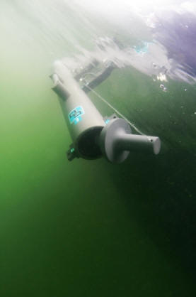
Figure 6.01 - Sampling using a Niskin Bottle
Introduction
Aims:
To understand how vertical mixing properties and nutrients directly and indirectly affect the functional properties of plankton communities.
Logistics
Date: 09/07/2008
Location: Inshore
Time: 0800 – 1330 GMT
Tide: HW 0947, 4.7 m
LW 1604, 1.4 m
Range: 3.3 m, Neap Tide
Conditions: 8/8 cloud cover, drizzle to rain all day, 8m/s SW wind
The Team:
Bill Conway
PSO – Mat
Computers – Bill
Scribe – Jess
Chemical sample processing – Natalia, Hannah
Stern deck – Scotty, Ed
Ocean Adventure
Deputy PSO – Alex B
Scribe / deployment – Alex S, Annabelle
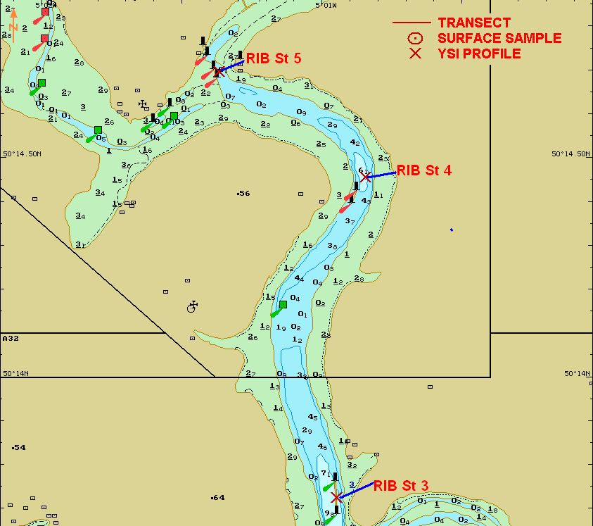
Bill Conway Method
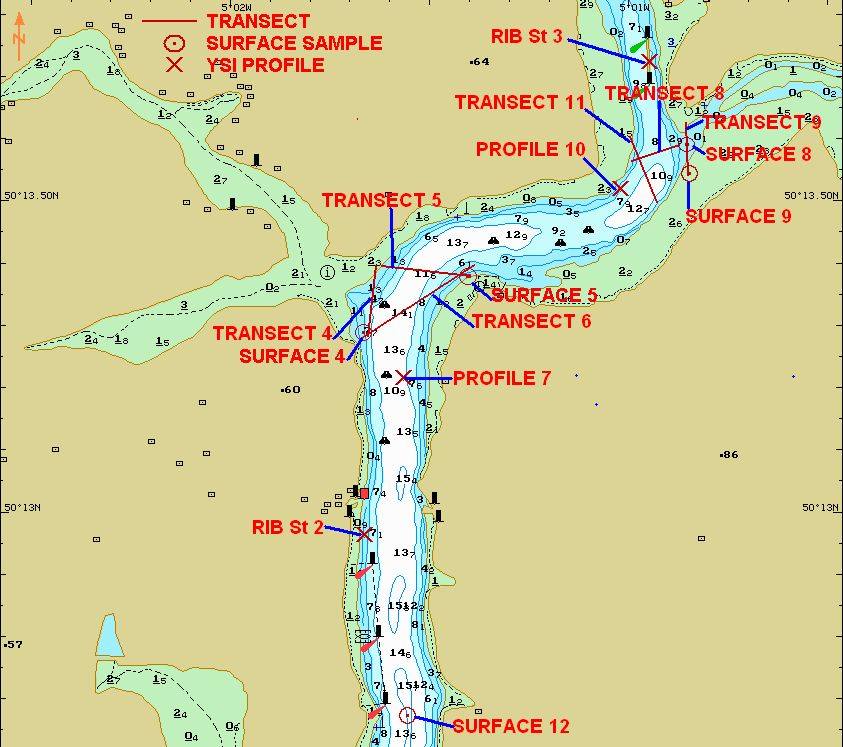
Sampling was planned to commence at Black Rock but due to large swell an ADCP transect was not possible. Therefore plans were changed and moved further up the estuary to begin sampling. At each transect data was recorded as an ADCP transect and surface samples and YSI profiles were taken at points of interest. The transects were as follows;
Between Penarrow Point and Messack Point,
North of Restronguet Creek travelling eastward
North of Channals Creek to Turnaware Point
Triangle shape North of Lamouth Creek
L shape across the Truro River input
Across front found up river
Vertical profiles were manually logged using the F98D YSI attached to a rosette. Niskin bottles were fired at appropriate depths and water samples were taken from them. From these samples;
a sample for dissolved oxygen was taken before any other contamination could occur and was fixed using Winkler reagents, 1ml Manganous Chloride and 1 ml Alkaline Iodide
100ml was stored for phytoplankton analysis with 1 ml Lugols Iodine,
50ml was filtered through glass fibre filter and sorted in glass bottles for nitrate and phosphate analysis,
50ml was filtered through a glass fibre filter and stored in plastic bottles for silicate analysis.
The filters used in the preparation of the nutrient samples were placed into acetone to extract the chlorophyll overnight. The surface samples were analysed in a similar way without samples for dissolved oxygen and plankton. At the first and last positions a 50 cm diameter, 200μm mesh plankton net was towed behind the vessel for 1 minute and the amount of water flowing through was measured using a flow meter. Zooplankton was preserved by adding Formalin. The euphotic depth was measured using a Secchi disk and the cloud cover was noted.
Ocean Adventure RIB Method
Stations were sampled at the following positions on the Ocean Adventure RIB;
Tolcarne Creek
King Harry Passage
Polgerran Wood
Woodbury Point
Malpas Point
At each station the vertical temperature and salinity profile was measured using a handheld F200 YSI probe. A Niskin bottle was used to take a water sample from just below the surface at each station. Water samples were taken from the Niskin bottle, and stored using the procedure described above. The filters used when filtering were again placed in acetone to extract chlorophyll. The salinity of the water in the Niskin bottle was recorded using the F200 YSI, so the samples could be correlated to the temperature salinity profiles. At stations 1, 3 and 5 oxygen samples were also taken from the, using the above treatment procedure. At stations 3 and 5 plankton nets were used to gather zooplankton samples, which were then preserved in Formalin. At station 3, the net was towed at the surface for 3 minutes at a speed of 1 knot. At station 5 the plankton net was placed just below the surface and held in the current of 0.25m/s for 10 minutes.
|
|
|
Introduction to the estuarine physics
The physical description of the estuary has been considered in two parts. The first examines the water fluxes and current flows within Carrick Roads and the Rivers Truro and Fal, and the second discusses the vertical structure and mixing within the system.
Discharge Fluxes
Flux rates were obtained from WinRiver, and both measured flux and estimated total flux have been tabulated (Table 6.01 below). Measured fluxes were those derived from the ADCP measured flow, estimated fluxes include corrections calculated by the program to represent the non observed parts of the channel. It should be noted that the ADCP did not profile to the seabed in transects 1 and 2 hence the flux data should only be considered as indicative of total flux.
The start time of each transect is shown, as is the time in relation to HW Falmouth. The obtained results appear largely consistent with the tides.
The transect positions are shown on Figs 6.02, 6.03, 6.04. Transect 1 shows a significant flood flow, the ADCP velocity direction contour plot (Fig 6.05) shows a North Westerly flowing water mass in the main channel. The channel is orientated NW / SE at this transect and so the observed flow is as expected at the end of the flood. The plot also shows a generally Northerly flow in the shallows to the west of the main channel, however there is a surface flow (to depth aprox 3m) to the NE, which is probably due to the strong South Westerly winds experienced throughout the day.
Transect 2 coincided with HW and the low flux is indicative of slack conditions. The observed velocities were all below 0.125 ms-1 and there did not appear to be a consistent flow direction.
Transects 3, 5, and 6, all of which cross the main river, do not appear consistent because the flux would be expected to increase downstream due to additions from tributaries. The observed fluxes could be partially explained by the development of the ebb
flow with increasing time after HW. However the differences between transects 5 and 6 cannot be accounted for by this time delay and may be due to errors in the WinRiver edge estimates.
There is some ambiguity with transect 3, it is probable the start and stop sides were incorrectly entered onboard. The discharge flux shown above has been corrected to give an ebb flow, however it is proving difficult to interpret the transect plots.
Transect 4 across Lamouth & Cowlands creeks shows a small ebb flow.
Transects 5 and 6 both show an ebb flow at depth, however the surface layer in both cases is slower, which may be due to retardation caused by the South Westerly wind. The observed wind speed was 8ms-1 which would be expected to cause a surface flow of 0.16 ms-1 (2% of wind speed). This can be seen in Fig 6.06 , which shows this velocity magnitude at transect 6, and it is clear that there is a surface flow which has been retarded by approximately 0.13 ms-1.
Transects 8 and 9 were across the Truro and Fal rivers respectively. The flux data show that the Truro river ebb flux is very approximately double that of the Fal.
Transect 11 was made across a streak of surface scum trailing South Westerly from the headland at the confluence of the Truro and Fal rivers. A very clear backscatter maximum was observed to a depth of 7m, at the position of the streak (see Fig 6.07). No other ADCP signal was observed, and it was not possible to sample the water column due to time constraints. It is unclear what the exact cause of the feature was, however it is possible that it was a front associated with the confluence of the two rivers, and that the ADCP resolution was insufficient to detect it.
| Description | Transect | Measured flux (m3/s) | Total Estimated flux (m3/s),+ve seaward | Time (Z) | Time to HW | ||
| Carrick Roads seaward | 1 | -552.34 | -985.72 | 08:27 | 01:20 | Before | |
| Carrick Roads Top | 2 | 29.31 | 69.76 | 09:28 | 00:19 | Before | |
| Turnaware Point (Narrows) | 3 | 242.65 | 309.41 | 10:07 | 00:20 | After | |
| Triangle - Lamouth Creek | 4 | 12.17 | 4.24 | 10:34 | 00:47 | After | |
| Triangle - main channel, above | 5 | 324.61 | 409.47 | 10:36 | 00:49 | After | |
| Triangle - main channel below | 6 | 280.95 | 333.3 | 10:42 | 00:55 | After | |
| Truro River | 8 | 192.13 | 260.15 | 12:06 | 02:19 | After | |
| Fal River | 9 | 87.47 | 162.86 | 12:09 | 02:22 | After |
Table 6.01, WinRiver discharge fluxes
Vertical structure and mixing
The vertical profiles at stations 1,2 & 3 appear to show a well mixed water column with a slight decrease in temperature and increase in salinity with depth (see Fig 6.25, Fig 6.26 and Fig 6.27, below). However, calculations of the Richardson number for these stations (see Table 6.02) suggest that there are layers with greater stability at a depth of 4, 3 & 2m at stations 1, 2 &3 respectively.
|
|
|
|
Transect 1 |
|
Transect 2 |
|
Transect 3 |
|||
|
Depth (m) |
Ri |
|
Depth (m) |
Ri |
|
Depth (m) |
Ri |
|
1.65 |
0.0000 |
|
1.65 |
0.0000 |
|
1.65 |
0.0000 |
|
2.15 |
0.0926 |
|
2.15 |
0.0244 |
|
2.15 |
99.0000 |
|
3.15 |
0.0115 |
|
3.15 |
2.7040 |
|
3.15 |
2.3437 |
|
4.15 |
3.3814 |
|
4.15 |
31.1250 |
|
4.15 |
0.1955 |
|
5.65 |
0.6736 |
|
5.15 |
5.5310 |
|
5.15 |
3.7848 |
|
6.15 |
0.0488 |
|
6.15 |
17.4106 |
|
6.15 |
0.0691 |
|
7.15 |
0.8251 |
|
7.65 |
0.0546 |
|
7.15 |
0.1813 |
|
8.15 |
16.2392 |
|
8.65 |
0.0722 |
|
8.15 |
0.0514 |
Table 6.02, Ri numbers at stations 1,2 &3.
![]()
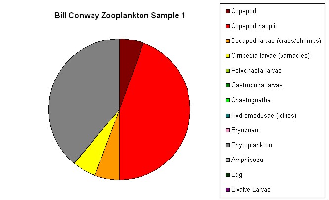
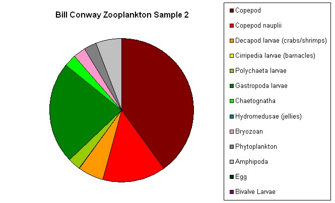
Sample 1 and 2, taken off the Bill Conway, were in the vicinity of transect 1, near Messack Point, and transect 11, near the River Fal and River Truro confluence, respectively.
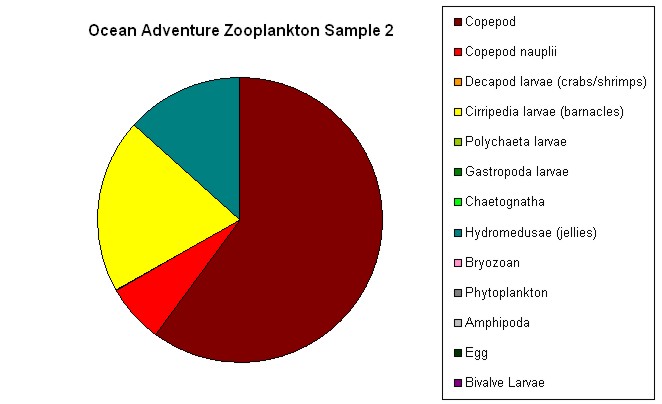
Sample 1 and 2, taken off Ocean Adventure, were upstream from station 3 and upstream from station 4 on the River Truro.
Sample 2 from Bill Conway had the highest number of organisms, 1268 m-3. The Ocean Adventure samples had significantly fewer organisms, at 111 and 25 m-3. Sample 2 off Bill Conway also had the greatest variety of organisms identified (9 groups). Ocean Adventure sample 1 has a higher number of groups than sample 1 off Bill Conway, six rather than five, also a highest proportion of copepods out of the four samples; although within sample 2 off Bill Conway the number of copepods per m3 was 6.8
times more than sample 1 off the Ocean Adventure. Within the alquiot of sample 1 off Bill Conway (Fig. 6.08), a similar proportion of visible phytoplankton and copepod nauplii were identified (approx. 40%). The high organism numbers in sample 2 from Bill Conway (Fig. 6.09) was made up of high percentages copepods (40%) and gastropod larvae (23%). The Ocean Adventure samples (Fig. 6.10 and Fig. 6.11) contained no decapod larvae, chaetognatha, phytoplankton, amphipoda or eggs. Copepods contributed to the majority (<60%) in both samples. Hydromedusae were the only other group that was present in both samples.
![]()
|
|
|
|
|
|
|
|
|
|
|
|
|
|
|
||
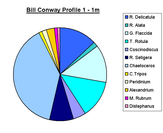
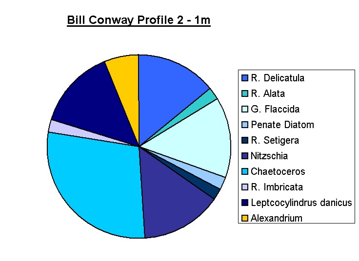
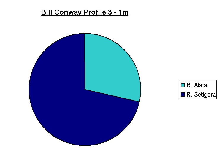
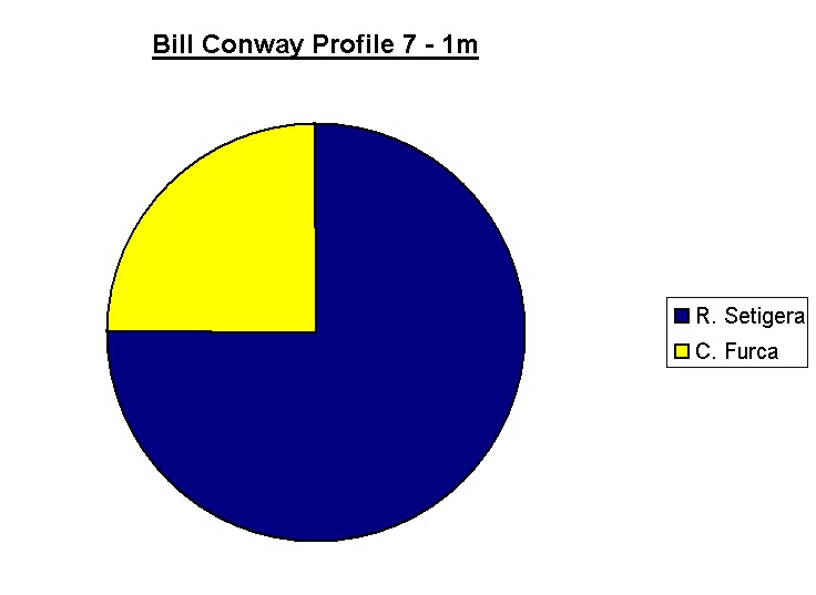
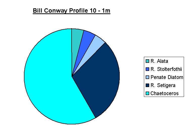
Each of the phytoplankton samples from Bill Conway and the RIB were found to contain a majority of diatoms (blue shades of pie charts), followed by dinoflagellates (yellow/orange shades) and then the ciliates (pink shades). Bill Conway profile 1 (Fig 6.12) was composed 89% of diatoms, profile 2 (Fig 6.13) 94% of diatoms and profile 3 (Fig 6.14) sample was composed only 100% diatoms of only 2 species R.Setigera, R.Alata. The sample from profile 7 (Fig 6.15) only contained two species as well, the diatom R.Setigera and dinoflagellate C. Furca. The sample at profile 10 (Fig 6.16) was composed of only 5 species of diatoms.
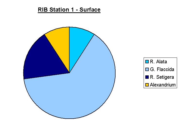
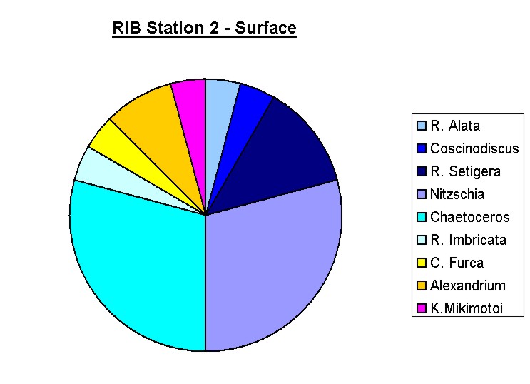
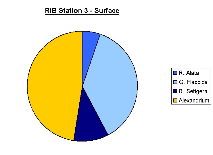
The species diversity is higher for the Bill Conway Samples than the Ocean Adventure samples, 19 species to 14 species identified. For the Bill Conway G. Flaccida was the dominant species found at each stations apart from station 2 where R.Alta and Chaetoceros were the dominant species present in the same numbers. At each of the RIB Stations there were dinoflagellates present and at stations 2 and 5 (Fig 6.18 and Fig 6.21) there were also ciliates present.
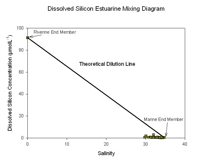
Dissolved Silicon
Dissolved silicon acts non-conservatively in the Fal Estuary as shown in the estuarine mixing diagram (Fig 6.22). Silicon is taken out of the system at high salinities, above 29, as shown by the points plotting below the theoretical dilution line.
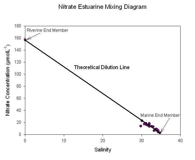
Nitrate
The estuarine mixing diagram for nitrate (Fig 6.23) shows that Nitrate behaves conservatively with points plotting close to the theoretical dilution line at the salinities measured.
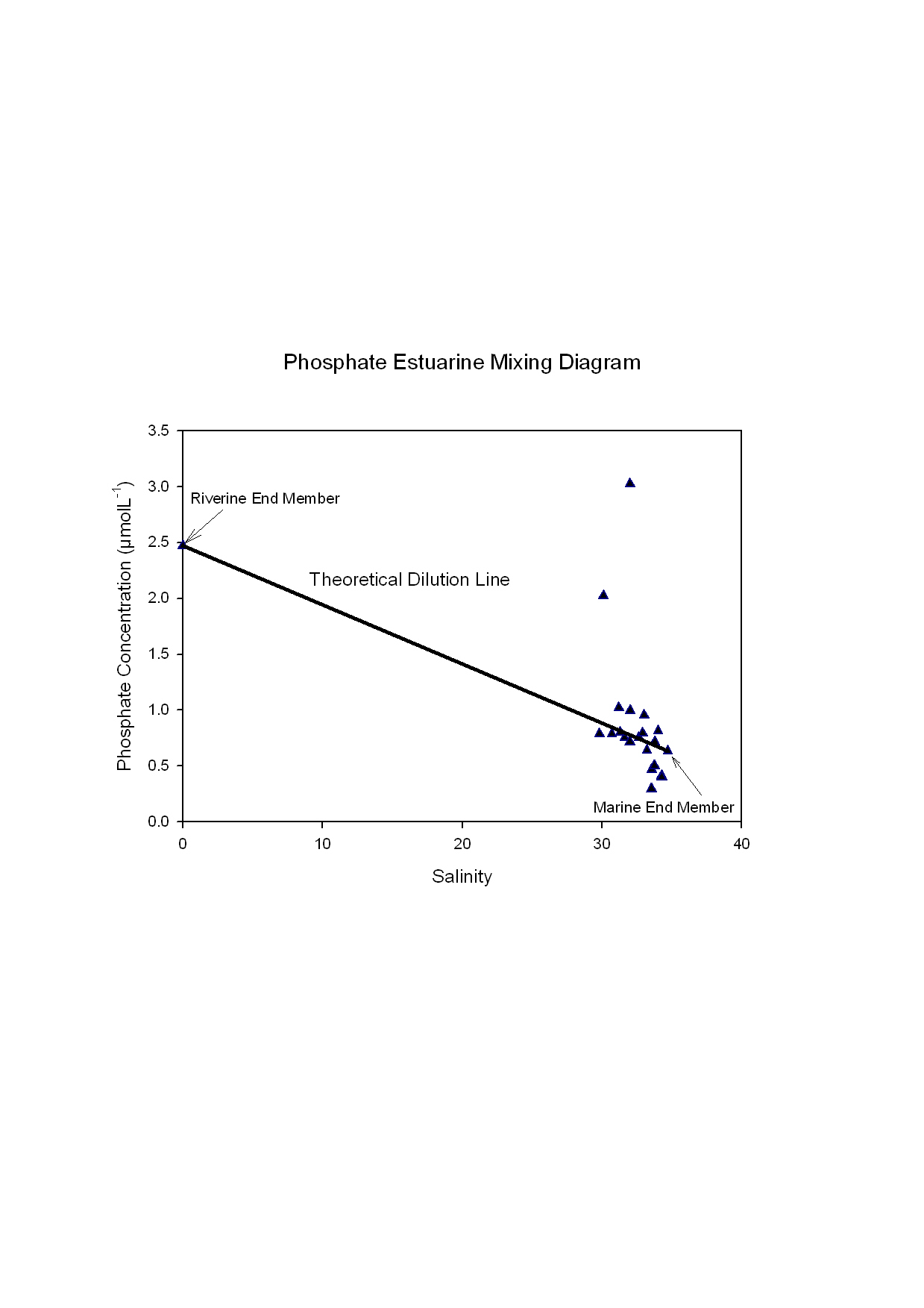
Phosphate
It can be seen from the estuarine mixing diagram (Fig 6.24) that there is an input of phosphate to the estuary at the lower salinities, 30 to 32, shown by plots lying slightly above the theoretical dilution line. There are possible anomalies at salinities of 30.5 and 32, with concentrations of 2.2μmolL-1 and 3.1μmolL-1 respectively, which are positioned outside the main range.
Dissolved Oxygen
Due to time restraints, few oxygen samples were taken. Therefore the data gathered is too sparse to analyse and no definitive trends can be seen.
![]()
|
|
|
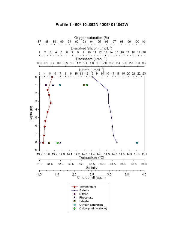
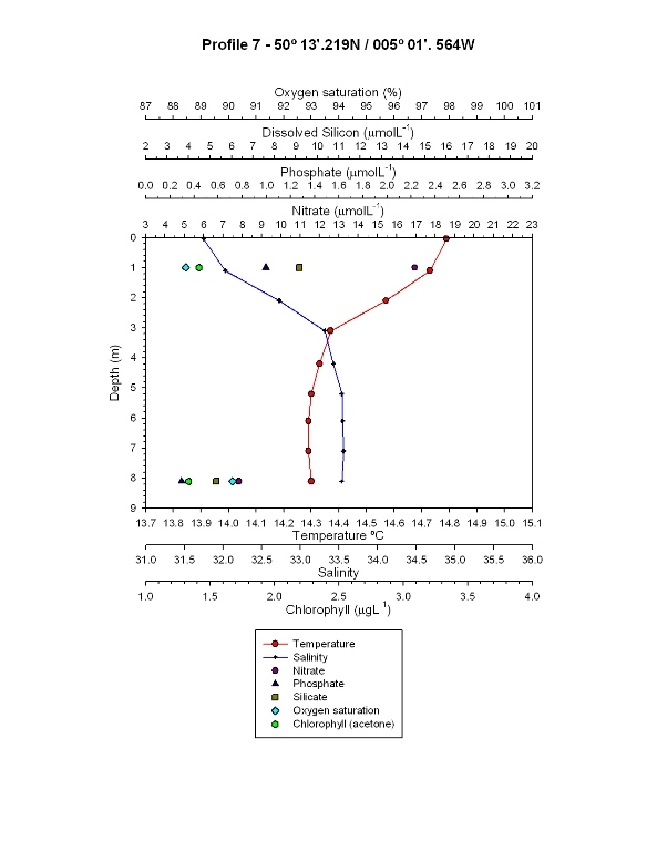
Oxygen saturation is greatest at the surface (92%) despite chlorophyll being lowest at the surface. Saturation decreases to 89.7% at maximum sampling depth (8.1m).
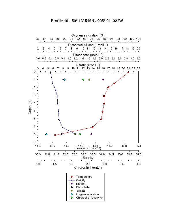
Profiles 7 and 10 (Fig 6.28 and Fig 6.29) both show the strongest stratification with a thermocline structure with depth. The temperature at profile 7 has a range from 14.8 °C at 0.04m depth to 14.3 °C at 8.1m. The salinity ranges from 31.8 at the surface to 33.5. All nutrients are shown to decrease with depth. Profile 7 has the highest surface nitrate of all stations with 16.9 µmol L-1 at the surface, falling to 7.8 µmol L-1 at 8.1m depth. This site has the highest surface phosphate ranging from 1.0 µmol L-1 to 0.3 µmol L-1. Dissolved silicon ranges from 9.2 µmol L-1 to 5.3 µmol L-1. Chlorophyll has a slight decrease from 1.4 µg L-1 at the surface to 1.3 µg L-1 at 8.1m. Oxygen saturation increases with depth from 88% to 90%.
Proflie 10 (Fig 6.29) has the highest surface temperature with 15 °C, decreasing to 14.5 °C at 8.1m. Salinity increases from 31.2 to 32.6 at maximum sampling depth. Like station 7, all nutrients decrease with depth. Nitrate decreases from 16 µmol L-1 at the surface by 2.3 µmol L-1, phosphate decreases from 0.8 µmol L-1 to 0.75 µmol L-1 at 8m depth. Dissolved silicon declines from 11.2 µmol L-1 at the 1m to 8.6 µmol L-1 at 8m depth. Chlorophyll shows a slight decrease from 2.35 µg L-1 to 2.25 µg L-1 and dissolved oxygen decreases with depth from 90% at 1m to 87% at 8m depth.
|
|
|
|
|
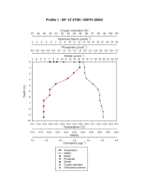
All profile stations show an increase in salinity with depth and a decrease in temperature with depth.
Profile 1 (Fig 6.25) shows salinity increases from 33.5 at the surface to 34.7 at 8.1m depth. There is a slight decrease in temperature with depth from 13.9 °C to 13.75 °C at 8.1m. Nitrate decreases by 1.3 µmol L-1 over 8.1m and phosphate increases with depth from 0.4 µmol L-1 to 0.6 µmol L-1 at 8.1m. Dissolved silicon shows a strong decrease between the surface at bottom samples from 9.1 µmol L-1 to 2.8 µmol L-1. Chlorophyll concentration diminishes from 2.4 µg L-1 at 1m to 1.52 µg L-1 at 8.1m. Oxygen saturation is 89.7% at the surface to 100% at depths.
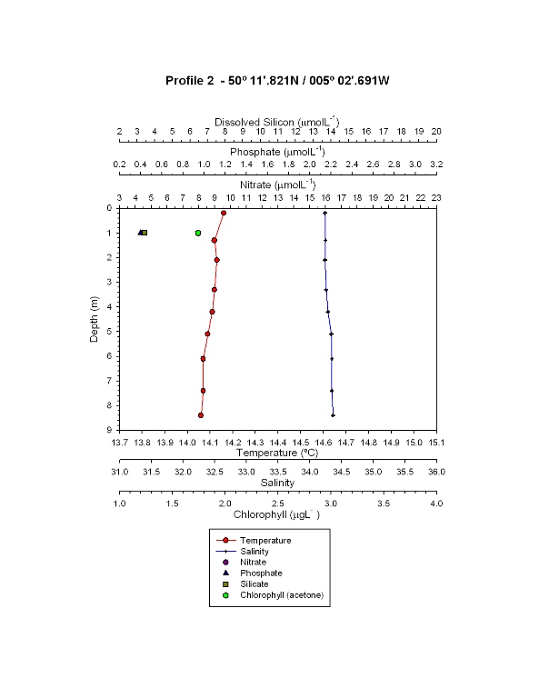
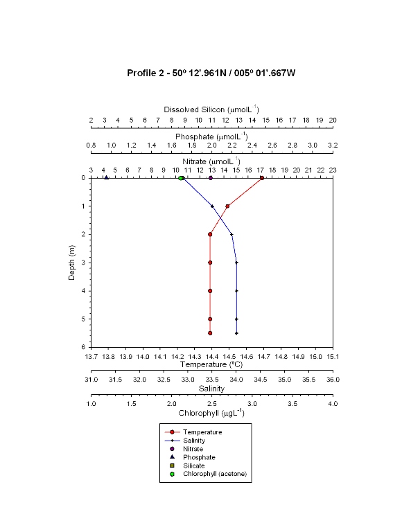
Fig 6.26 shows the most stable profile of temperature and salinity with depth with very little change overall (change of 0.1 units for each) was at profile 2. Only a surface sample was taken so there is no comparison of nutrients and oxygen with depth. At the surface
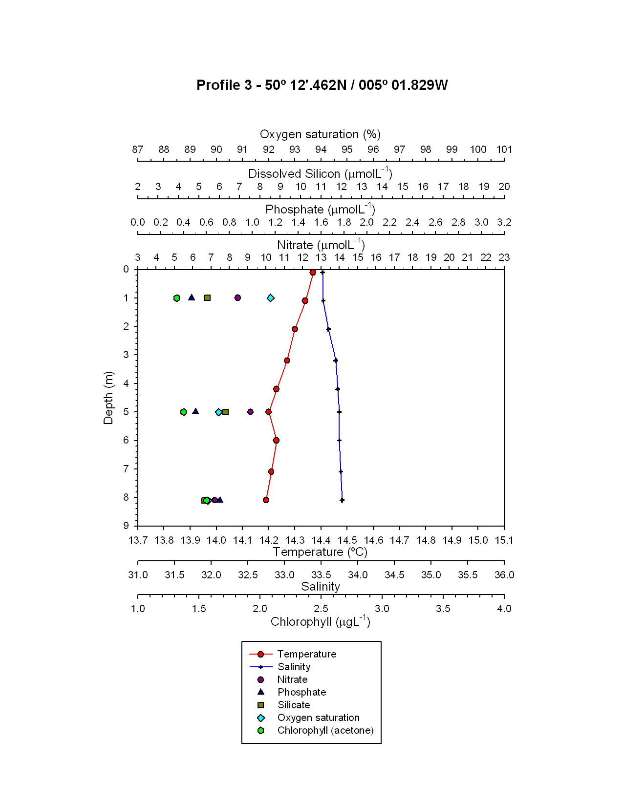
Profile 3 (Fig 6.27) shows an increase in salinity with depth and temperature decreases with depth like all profiles taken on Bill Conway. Chlorophyll increases with depth from 1.32 µg L-1 at the surface, to 1.57 µgL-1 at 8.1m depth. Nitrate decreases by 1.3 µmol L-1 from 8.5 µmol L-1 at 1m. Phosphate increases with depth by 0.2 µmol L-1 from 0.5 µmol L-1 at 1m, and silicon has a maximum at 5m depth with 6.3 µmol L-1.
Station 4 (Fig 6.33)
Like the previous stations, the temperature decreased with depth throughout the water column. The surface temperature was 15 ºC and decreased to 14.3 ºC at a depth of 8.7m. There was no change in temperature below a depth of 5.2m. The salinity change at station 4 increased with depth from a surface salinity of 31.5, to 34.1 at a depth of 8.7m.
The dissolved silicon concentration in the surface waters at station 4 was 19.19µmolL-1. The phosphate concentration, again taken from the surface, was 2.02µmolL-1. The surface nitrate concentration at station 4 was 22.83µmolL-1.
Chlorophyll concentrations were again taken from surface water samples. The chlorophyll concentration at station 4, in the surface waters was 4µgL-1.
Station 5 (Fig 6.34)
Unlike the other stations, there was no decrease in temperature with depth at station 5. The temperature throughout the water column at station 5 remained constant at 14.8 ºC. The salinity change at station 5 was similar to the other station, with salinity increasing with depth. The surface salinity was 32.1 and increased to 32.4, at 4.5m depth.
The oxygen saturation, taken from a surface water sample, at station 5 was 88%. The dissolved silicon concentration at station 5 was 16.79µmolL-1. The phosphate concentration at station 5, again taken from a surface water sample, was 3.02µmolL-1. The surface concentration of nitrate at station 5 was 18.52µmolL-1.
The chlorophyll concentration was again taken from a surface water sample and was 2.76µgL-1.
RIB Results
Station 1 (Fig 6.30)
The temperature data shows a clear trend between temperature and depth; as the depth increases the temperature decreases. The temperature at the surface was 14.5ºC and decrease to 13.9ºC at a depth of 9.4m. As with temperature, there is a clear trend between salinity and depth, however unlike temperature, salinity increases with depth, but this is what is expected at this position. At the surface the salinity was 34 and increases to 35.2 at a depth of 9.4m.
The only oxygen sample was taken at the surface (using a Niskin Bottle). At the surface the oxygen saturation was 94%. Similar to oxygen, the only sample of dissolved silicon taken was at the surface, again using a Niskin Bottle. The surface concentration of dissolved silicon was 5.8µmolL-1. Phosphate concentrations were also taken at the surface using a Niskin Bottle. The concentration of phosphate at the surface was 0.81µmolL-1. The nitrate concentration, again taken at the surface with a Niskin Bottle, was 8.8µmolL-1.
The chlorophyll concentration, as determined due to filtered water samples being placed in 90% acetone, was also taken from a surface water sample, using a Niskin Bottle. The Chlorophyll concentration in the surface water was 2.12µgL-1.
Station 2 (Fig 6.31)
The temperature data again shows a clear trend between temperature and depth; as the depth increases the temperature decreases. The temperature at the surface was 14.7ºC and decreased to 14.4ºC at a depth of 5.5m. There was no change in temperature, however, below a depth of 2m. Again, there is a clear trend between salinity and depth. At the surface the salinity was 32.9 and increases to 34 at a depth of 5.5m. There was no change in salinity after a depth of 3m.
The concentration of dissolved silicon, which was again taken from the surface, was 8.8µmolL-1. Phosphate concentrations were also taken at the surface using a Niskin Bottle. The concentration of phosphate at the surface was 0.95µmolL-1. The nitrate concentration taken at the surface was 12.9µmolL-1.
The chlorophyll concentration, from a surface water sample, was 2.11µgL-1.
Station 3 (Fig 6.32)
At station 3 the temperature profile was similar to both station 1 and 2. The temperature decreased with depth, from a surface temperature of 14.7 ºC down to a temperature of 14.2 ºC at a depth of 10m. The salinity increased with depth, just like at stations 1 and 2. The surface salinity was 32.9 and increased to 34.3, at a depth of 10m.
The surface oxygen saturation at station 3 was 89%. The surface concentration of dissolved silicon was 12.88µmolL-1. The surface concentration of phosphate at station 3 was 0.79µmolL-1. The surface concentration of nitrate at station 3 was 13.04µmolL-1.
The acetone chlorophyll concentration at station 3, which was taken from a surface water sample, was 2.47µgL-1.
|
|
|
|
|
|
The estuaries data differs from the offshore data as the areas of high chlorophyll tended to be areas of low oxygen saturation, except for the furthest upstream stations. There was high biological oxygen demand, due to high levels of nutrients. Temperature decreased with depth at all the stations, apart from RIB station 5, which was the furthest upstream, the shallowest and had the least marine input. Salinity increased with depth, due to the less dense fresh water at the surface from inputs from the Fal and its tributaries. There was high precipitation throughout the week increasing riverine input and direct freshwater input to the estuary. The greatest change in depth was found in Bill Conway’s profile 7. The nutrients are generally high in the surface waters, due to it being an ebb tide, where river water dominates.
Oxygen decreased with distance upstream, whereas chlorophyll seemed to increase near the source and mouth of the river, decreasing in the central parts (shown by the chlorophyll extract values) showing there is an increase in phytoplankton at the source of the river and mouth of the estuary. Dissolved silicon rapidly increases the further inshore due to high silicon input from the rivers and uptake by diatoms at the seaward end.
Phosphate steadily increases the further inshore, due to uptake by phytoplankton at the mouth of the estuary. Nitrate behaves in a similar way to phosphate, due to the same reasons. Both phosphate and nitrate behave conservatively, whereas dissolved silicon behaves non-conservatively, due to removal downstream by diatoms. There are some anomalies with the phosphate data, which could be due to sewage effluence or simply problems with the data.
Profile 7 was near to the mussel beds. This profile showed increased nutrient concentrations and reduced flow, which may have been due to the mussel beds, or due to increased faecal coliforms, which enhance bacterial activity within the water column.
This webpage presents a summary of selected data, collected by group 4 during the 2008 Falmouth Field Course. The full dataset is available online at the Falmouth FTP site.
It is important to note that the study was somewhat constrained by the time domain. In order to establish a more complete picture of the region over the field work period, the data should be considered together with the datasets of the other eight groups. It should also be made clear that the results and discussions presented here are an initial analysis of a large dataset and are intended to give only a provisional overview of the data. If users intend to make comparisons between this data set and those obtained in previous years, it should be borne in mind that during the period of these observations the weather was unusually wet and windy.
Finally, we would like to acknowledge the advice and assistance given by the academic staff and boat crews.
Thank you for visiting our site,
Alex B, Alex S, Annabelle, Bill, Ed, Hannah, Jess, Mat, Natalia & Scott .
References
These references have been used directly and indirectly, through prior knowledge, in the formation of this website.
Foden, J., Purdie, D.A., Morris, S., and Nascimento, S., (2005) "Epiphytic abundance and toxicity of Prorocentrum lima populations in the Fleet Lagoon, UK". Harmful Algae, 4(6), 1063-1074.
Grasshoff, K., K. Kremling, and M. Ehrhardt. (1999). Methods of seawater analysis. 3rd ed. Wiley-VCH.
Johnson K. and Petty R.L.(1983) “Determination of nitrate and nitrite in seawater by flow injection analysis”. Limnology and Oceanography, 28 1260-1266.
Langston, W.J., Chesman, B.S., Burt, G.R., Hawkins, S.J., Readman, J. and Worsfold, P., (2003) "Site Characterisation of the South West European Marine Sites: Fal and Helford cSAC". Plymouth Marine Science Partnership.
Parsons T. R. Maita Y. and Lalli C. (1984) A manual of chemical and biological methods for seawater analysis 173 p. Pergamon.
White, N., (2004) "Marine Ecological Survey of the Fal Estuary: Effects of Maerl Extraction". Falmouth Harbour Commissioners.
www.bbc.co.uk/weather
www.easytides.ukho.gov.uk
www.eoearth.org/article/Seagrass_meadows
www.fdmarine.com
www.soes.soton.ac.uk/resources/boats
www.xcweather.co.uk
All websites accessed between 01/07/08 and 11/07/08.
The opinions and views expressed in this website do not necessarily represent those of the University of Southampton or the National Oceanography Centre, Southampton.