|


|
|
INTRODUCTION
|
During
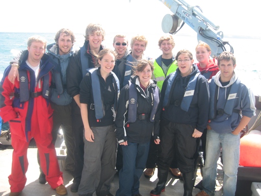
the first two weeks of July 2008 Group 3, eleven Oceanographers
and Marine Biologists, undertook an investigation into the
physical, chemical, and biological processes in the Falmouth
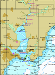
area. Falmouth is situated in the South West tip of England
in the county of Cornwall and is exposed to prevailing south
westerly winds from the Atlantic Ocean.
The
estuary is a Ria typified by steep-sided valleys common to
the majority of British estuaries. Falmouth is the third
deepest natural harbour in the world and it is fed by 6 main
rivers the Truro, Tresillian, Pill Creek, Restrongruet
Creek, Mylor Creek and Penryn River as well as many smaller
creeks and tributaries.1 However, the volume of
freshwater delivered to the estuary is small, suggesting the
effect of freshwater on estuarine condition is negligible.
The estuary is well-mixed and varies in tidal range, with
the main body being predominantly mesotidal (2-4m).
One of
the most metal polluted areas in Britain, the Fal has been
exposed to high levels of copper, zinc and cadmium mainly
through agriculture and mining activity. In the past this
has had an adverse effect on the biology leading to the area
becoming a Candidate Special Area of Conservation.
The Fal
estuary and the offshore region were surveyed using four
research vessels, Callista, Explorer, Bill Conway, and Ocean
Adventure. As the estuary itself is a dynamic environment
varying seasonally, temporally, and spatially a variety of
measurements were undertaken.
Please browse our website
for our findings
from the estuary and
offshore area!
|
|
VESSELS
|
RV Callista
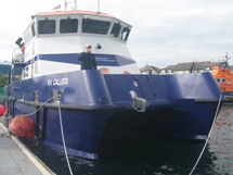
Day boat used for sampling both the
Estuary and Offshore
Length:
19.75m
Beam: 7.4m
Draft: 1.8m
Speed: 15 knots
Passengers: 30 max
A-Frame: 4 tonne capacity
Capstan: 1.5tonne pull
Davits: 2x100kg
Range from safe haven: 60mls
|
RV Bill Conway
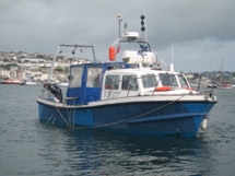
Day boat used for sampling the Estuarine Area
Length:
11.74m
Beam: 3.96m
Draft: 1.3m
Speed: 9knots
Passengers: 14 including crew
A-Frame: 750kg
Davits: 1x50kg
Trawl Winch: max wire length 70m
Range from safe haven: 60mls
|
|
RV Xplorer
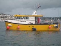
Survey boat used to scan the geophysics
of the Helford River area
Length:12.0m
Draft: 1.00m
Speed: 25 knots (max)
Passengers: 12 passengers plus crew
Capstan: Anchor retrieval
Range from safe haven: 60 mls
|
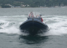
Ocean Adventure (RIB)
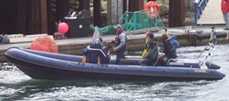
RIB used to sample the upper reaches of the
Estuary and the Fal River
Length: 7.0m
Beam: 2.55m
Draft: 0.5m
Speed: 35knots max
Passengers: 6
Range: 20mls from safe haven
|
Back to top
EQUIPMENT
|
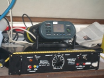
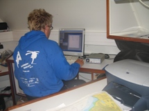
ADCP-Acoustic
Doppler Current Profiler
ADCP sends out
pulses of sound that are received back as echoes at varying
times depending on current properties. Data on current
velocity and direction is received via an on-board computer
using the program WinRiver Aquirer and is processed further using the
program WinRiver Playback. Backscatter readings indicate
turbidity and presence of biology within the water column.
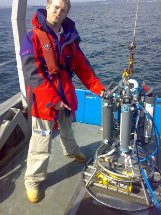
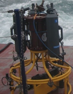
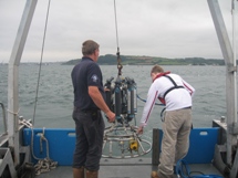
CTD –
Conductivity, Temperature and Depth Profiler
The CTD gives a
vertical profile of the water column. For Bill Conway, the set up used consisted of six GoFlo
Bottles used to take water samples loaded on a Rosette with
an attached YSI Probe (F105c). The CTD is deployed using a winch with communication with the onboard
computer showing depth of the water column.
Both an up-cast and a down-cast were sampled,
with the GoFlo Bottles being fired via remote onboard
computer, at depths determined from the down-cast.
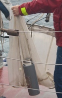
Zooplankton
Net
The net used had
an entrance diameter of 0.4m and a mesh size of 200µm. The
net is towed behind the vessel and a Hydro Bioskiel counter
is used to measure the amount of water flowing through the
net. The sample is collected in a vessel attached to
the net and the net is rinsed with water from the onboard
pump into the collection vessel.
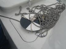
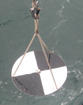
Secchi Disk
The secchi disk
is used to determine the depth of the euphotic zone (1%
light level) of the water column. The disk, approximately
20-30cm, has alternating black and white panels. The disk
is lowered until not longer visible, this depth is
multiplied by 3 to get the depth of the euphotic zone. The
disk should be operated by the same individual at each
station to avoid discrepancies.
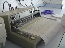
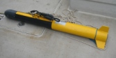
Side-Scan
Sonar - Geo Acoustics Ltd (159D)
The side scan sonar
device, also known as a ‘tow fish’, was towed behind Xplorer
and emitted a sound pulse at a frequency of 100kHz. The
pulse emitted was reflected off of the seafloor and returned
to the towfish, resulting in a black and white image. The
darker lines represent stronger reflections, which indicate
sediment types such as coarse sand. Lighter lines are often
indicative of mud or silt. The side scan image can also show
depressions and elevations in the seafloor.
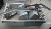
Van Veen Grab
The Van Veen Grab is a lightweight long-levered sediment
sampler that takes large samples of soft sediment. The
sample size used was 0.5m3.
Back to top
|
|
WORKING IN THE ESTUARY
|
Aims
RV Bill Conway and Ocean Adventure (RIB) were used to take
measurements in the estuary from Malpas to Black Rock.
The aims of this section are to:
- Estimate
and compare the phytoplankton abundance from surface
samples taken
at stations ranging from Malpas to Black
Rock.
- Understand
how the physical, chemical and biological parameters change
within
the estuary and to suggest reasons for the
distribution of these parameters, which
include temperature,
salinity, dissolved oxygen, turbidity, and chlorophyll.
- Determine
how nutrient levels changed as a result of pollution inputs
from both
point and diffuse sources and biological activity.
Method
RIB
Ocean Adventure started at Malpas, the RIB's upper limit in the
estuary, in order to move against tidal flow so that the
same body of water was not sampled twice. A depth profile was taken
using two separate YSI probes, YSI 6600 is a 5 parameter
(Temperature, salinity, chlorophyll, turbidity, oxygen
saturation) multiprobe and YSI 650 is a two parameter
multiprobe (Temperature, salinity). Water samples were taken
to determine the silicon, nitrate, and phosphate
concentrations at every location and bottles were collected
to determine the oxygen percent saturation at 4 locations.
Samples were taken using a hand-held Niskin bottle triggered
at a depth of 0.5m. Salinity was
monitored continuously with the aim of selecting optimum
sampling stations as the RIB travelled down the estuary to Turnaware Point.
For the most part, buoys and
pontoons were used for convenience, safety, and positioning.
A total of 6 stationary samples were taken and one sample
was collected in a bottle while the RIB was moving due to a
lack of fixed mooring positions. The wrong net was provided
so zooplankton samples could not be collected on the RIB.
Using bottles filled with Lugols, phytoplankton samples were
collected at 4 locations for analysis to determine the
phytoplankton abundance and species present at each
location.
Conway
RV Bill Conway headed to Black Rock and carried out a
transect and a depth profile using an ADCP and a CTD (the
set up used consisted of a T/S probe attached to a rosette). Water
samples, zooplankton samples, and phytoplankton samples were
taken at this location to be analysed in the same manner as
the samples collected on the RIB. The vessel then moved
to Smuggler’s Cottage, the highest point up the
estuary for the vessel. Transects 2, 3 and
4 were carried out to form a triangle to determine the
effect of the river inputs in this area. A CTD was deployed
at the middle of transect 2 and water samples, zooplankton
samples, and phytoplankton samples were taken at this
location. The vessel travelled back down the estuary and
carried out another 5 transects and CTD depth profiles down
to Falmouth Harbour. No samples were taken at CTD stations 3
and 7, however surface samples were taken at 0.5 salinity
intervals.
Transect Positioning Data for Bill Conway
|
Transect |
Latitude |
Longitude |
Time (GMT) |
Start distance from
shore (m) |
Finish distance
from shore (m) |
|
Start |
Finish |
|
1 |
50°08.588 N
50°08.495N |
005°02.442W
005°01.149W |
09:04 |
09:16 |
108 |
107 |
|
2 |
50°13.432N
50°13.385N |
005°01.556W
005°01.414W |
10:49 |
10:51 |
34 |
81 |
|
3 |
50°13.397N
50°13.276N |
005°01.400W
005°01.664W |
10:53 |
10:57 |
40 |
28 |
|
4 |
50°13.397N
50°13.276N |
005°01.649W
005°01.482W |
11:00 |
11:02 |
38 |
83 |
|
5 |
50°12.506N
50°12.379N |
005°01.841W
005°01.790W |
11:48 |
11:51 |
7 |
16 |
|
6 |
50°12.277N
50°12.249N |
005°02.375W
005°02.217W |
12:10 |
12:12 |
34 |
90 |
|
7 |
50°11.590N
50°11.580N |
005°.03.034W
005°02.612W |
12:34 |
12:39 |
50 |
139 |
|
8 |
50°10.477N
50°10.884N |
005°02.537W
005°01.591W |
13:08 |
13:17 |
58 |
68 |
|
9 |
50°09.360N
50°09.375N |
005°02.877W
005°01.371W |
14:07 |
13:17 |
63 |
40 |
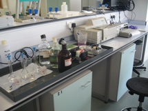
Laboratory Methods
Nutrient analysis was subdivided into the
analysis of chlorophyll, phosphate, nitrate, dissolved
silicon and oxygen concentration.
The chlorophyll was examined by fluorometry3, whilst the
phosphate and nitrate6 were examined by flow injection
analysis spectrophotometry, with nitrite being measured as a
representative of nitrate. The silicon was also analysed
using flow injection analysis spectrophotometry with the
silicon being treated with reagent (ammonia molybdate) and
reducing agent (MRR; Metol Sulphite : Oxilic Acid :
Sulphuric Acid : MQ Water, at a ratio of 10:6:6:8
respectively). The data was analysed using two separate sets
of standards as the first set were unsuitable for the low
absorbance samples. The oxygen concentration was calculated
using the semi automated Winkler reagent method5.
Water samples were also analysed for phytoplankton and
zooplankton quantities. Having been left to settle
overnight, the phytoplankton samples were then analysed
after the sample had been concentrated (9/10 of the volume
of the sample was removed leaving the plankton who had
settled in the concentrated sample). The zooplankton samples
we analysed under a microscope using a Bogorov Counting
Chamber containing 5ml of sample.
|
Results/Discussion
Those stations analysed at the lowest
salinities show vary different physical, chemical and
biological structure to those analysed near the mouth of the
estuary.
Physics
Station Data
Station C1
Station C1 shows homogenous salinity,
the Richardson’s number shows laminar flow in the top layer
with shear created at the thermocline between layers. It
then fluctuates between laminar and turbulent in the deep
layer, thus creating the underlying well-mixed water body.
Station C4
Station C4 shows a slight thermocline
in the upper 4m of the water column, above which
laminar flow was present. Where the upper outflowing
freshwater layer meets the flooding saltwater, shear is
created, lowering the Richardson's number. Below this, the
water column is well mixed with temperature and salinity
homogenous with depth.
Station C6
Station C6 shows a well mixed water
column with salinity and temperature homogenous throughout.
Collected nutrient samples suggest they are unvarying in
concentration however, samples were limited to 3 depths
reducing the ability for reliable analysis.
Discussion
The stations nearer the head of the
estuary tend to have pronounced partially mixed structures
with strong haloclines occurring at stations R1 and R2
(Figure 4). In comparison, those stations located nearer the
mouth, for example C1 and C6 (Figures 1 and 3), demonstrate
greater homogeneity in salinities with depth. It can be said
therefore, that the Fal estuary is well mixed near the
mouth, but becomes progressively more partially mixed near
the head. This is probably a result of tidal dominance near
the mouth and the impact of the river near the head. It must
be noted however, that stations R1 and R2 were only sampled
during low tide. Therefore the real effect of the tide cannot be
derived from the results. Temperature also follows this
structure of increased stratification near the head and
homogenous distribution with depth near the mouth.
The ADCP data is illustrated in figure
7 and shows the progressive movement of the tide over the
survey. Transect 2 shows the most riverward transect,
indicating faster flow at depth. This shows the landward
movement of seawater at depth with the seaward river flow
above showing a stratified water column. Looking at transect
5, the point where the fast moving flooding tide meets the
freshwater is clearly seen as the stratification breaks
down, transect 6 showing the well mixed tide on the flood.
Transect 1 was taken at Black Rock, the most seaward
sampling area and shows a well mixed and slowing moving
water column, there is movement in and out of the estuary
due to a turbulent eddy caused by Black Rock. This transect
was taken at the beginning of the survey where the tide is
turning, the slack water clearly seen in this figure.
The current pattern corresponds to the
phytoplankton data (Figures 12 and 15), as the water column becomes
more mixed, the number of dinoflagellates decreases as mixed
conditions are damaging to the flagella whereas the number
of diatoms, that are more robust, increases.
| CTD Sample Number |
2 |
3 |
4 |
5 |
6 |
7 |
1 |
| Attenuation Coefficient (k) |
0.576 |
0.411 |
0.576 |
0.360 |
0.360 |
0.360 |
0.288 |
| Depth of Euphotic Zone (m) |
15+ |
7.5 |
10.5 |
7.5 |
12 |
12 |
12 |
Table 1: Secchi Disk results showing depth
of euphotic zone as 3x secchi disk depth and the attenuation
coefficient (k) - Transect 1 is positioned last as it was
sampled at Black Rock same as sample 7
Secchi disk data (Table 1) indicates
that the depth of the euphotic zone decreases around the
middle estuary. This can be explained by increased
confluence of several freshwater inflows at this point
increasing the sediment load. This was also the point where
the flooding tide met freshwater causing increased
turbulence (see Figure 7, ADCP 5). The attenuation
coefficient shows a general increase landward, where the
increased sediment load and increased numbers of
phytoplankton (Figure 12) led to faster attenuation of
available light.
Chemistry
Nutrient concentrations decrease with
increasing salinities. The estuarine mixing diagrams for
nutrients in the estuary show mixed results. The mixing
diagram for nitrate (Figure 8) shows active removal from the
water column, whereas silicon (Figure 9) and phosphate
(Figure 10) shows active addition. The addition of both
nutrients could be explained by the high levels of
precipitation occurring in the area over the period of the
survey and preceding days which would increase surface
runoff into the estuary. The removal of nitrate can be
attributed to the presence of dinoflagellates, particularly
Alexandrium (Figures 11 and 16) which has been previously
related to fluxes in inorganic nutrients, mainly nitrate (Amniot
et al 2001)2.
As nutrient samples were only taken at certain depths
depending on the data from the downcast, there is little
data to explain the vertical distribution of these nutrients
(Figures 1-6). Vertical profile 1 from Conway (Figure 1)
shows
a visible peak in nitrate which is echoed by phosphate below
the thermocline, as nutrients are limited above due to biotic
and abiotic factors such as stratification and utilisation
by phytoplankton. Chlorophyll is reduced at depth due to
light attenuation reducing the numbers of phytoplankton.
Back to
Estuaries
Back to top
|
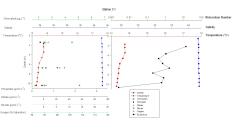
Figure 1: Conway Station 1 Vertical Profiles
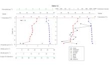
Figure 2: Conway Station 4 Vertical Profiles
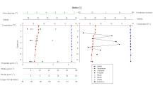
Figure 3: Conway Station 6 Vertical Profiles
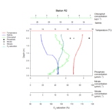
Figure 4: RIB Station 2 Vertical Profiles
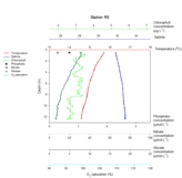
Figure 5: RIB Station 5 Vertical Profiles
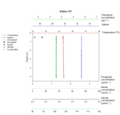
Figure 6: RIB Station 7 Vertical Profiles
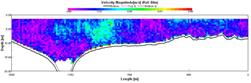
Figure 7: Estuarine ADCP data from Bill
Conway
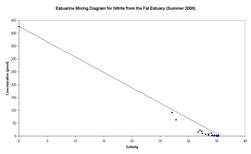
Figure 8: Nitrite Estuarine Mixing Diagram
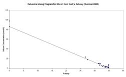
Figure 9: Silicon Estuarine Mixing Diagram
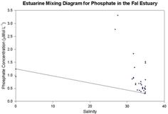
Figure 10: Phosphate Estuarine Mixing Diagram
|
WORKING OFFSHORE
|
Aims
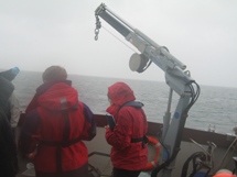
On 4 July 2008 group 3 went out on RV Callista to carry out
offshore measurements to better understand the chemistry,
physics, and biology of the offshore region.
The aims of this
section are to:
-
Estimate and compare phytoplankton and zooplankton
abundance from samples taken at various depths at stations
ranging from Carrick Roads to 3.5 miles offshore to help
understand the dynamics of the water column.
-
Determine the position of the front and how physical,
chemical and biological parameters change either side of
this and with distance from the shore.
-
Understand how the tidal movements affect the water
column in Carrick Roads.
-
Compare the results obtained in the offshore region
with those of the estuary.
Method
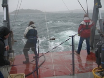
The
original plan for our day offshore was cut short by an
advancing weather system. The Force 5 increasing Force 7
South Easterly winds brought with it a 3 metre swell,
scuppering our original plans for offshore sampling.
Our transect instead lead us offshore from Black Rock on a 3
mile ADCP transect run, with a CTD downcast at the start, at
the 2 mile point and at 3 mile turnaround, to establish a
Vertical Profile. The Niskin Bottles were fired at the
surface, middle and bottom of the water column. At each of
these stations we also deployed 200µm mesh zooplankton net
and the samples preserved in formalin. A Secchi Disk was also
deployed and the cloud cover noted.
The initial sampling strategy was to use the running time
ADCP data to establish the presence of a tidal front at a
location offshore, and sample around it establishing its
characteristics and precise orientation.
After re-entering the estuary, a new estuarine sampling
strategy was adopted and transects across the estuary were
taken. CTD casts were sampled at the channels deepest point
and Secchi data was gathered as for the offshore sites. The
Zooplankton net samples were completed with a horizontal
tow, instead of the vertical lift adopted offshore.
For details of the Laboratory Methods used to analyse the
nutrients collected in the samples please
click here.
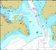
Transect Positioning Data for Callista
|
Transect |
Latitude |
Longitude |
Time
(GMT) |
| Start |
Finish |
| 1 |
|
|
005°01.633 W |
|
004°59.696 W |
|
09:35 |
10:10 |
| 2 |
|
|
005°03.165 W |
|
005°03.062 W |
|
12:32 |
12:35 |
| 3 |
|
|
005°03.062 W |
|
005°01.906 W |
|
12:35 |
12:43 |
| 4 |
|
|
003°03.161 W |
|
003°01.930 W |
|
13:17 |
13:29 |
| 5 |
|
|
003°03.153 W |
|
003°01.915 W |
|
13:42 |
13:55 |
|
|
Results/Discussion
For the offshore work, the ADCP and vertical profile data
have been analysed. The ADCP data corresponds to the
continuous transects and the vertical profiles correspond to
the CTD profiles taken.
ADCP Data
Looking in detail at
the ADCP data (Figures 11) several sections have been picked
out giving an overall picture of the water column during the
sampling. Figure 11 shows the ADCP data in detail. The first
transect taken, travelling between Black Rock and CTD 2,
positioned offshore, was taken at the point of an ebbing
tide. Tidal diamonds A and B were used to determine the
direction of tidal flow. The ship track shows a south
westerly flow which supports the data from these tidal
diamonds showing two interacting water masses. The ADCP
profile shows higher velocity flow at depth close to CTD 2
with the maximum velocities at 30-42m depth at 0.4-0.5ms-1.
At mid-way along the shelf the water velocity begins to
increase with a transition from 0.1-0.3 ms-1;
this continues offshore.
The backscatter profile for this transect shows consistently
high levels at the surface, around 90dB. This may be
indicative of large populations of zooplankton but at this
location is more likely to be caused by wave action due to
the rough weather. The Richardson number of 0.1 at Black
Rock correlates with this data indicating turbulent flow,
however backscatter is much lower (67dB) toward Black Rock
indicating a well-mixed vertical profile. Less backscatter
correlates with the increasing velocity as there will be
higher levels of mixing giving smaller populations of
zooplankton, but at 4815m offshore, there is a slight increase in
backscatter, from values around 69dB to 74dB. This could
indicate the beginning of a frontal system. This would be
more evident if there was less mixing.
Transect 2 looks at the
period between CTD 2 and CTD 3 and indicates an increase in
velocity from 0.5-0.7ms-1 during the second 1000m
of the transect as it continued offshore. The increased
influences of wind and wave could be responsible for this
change.
The backscatter profile here shows high levels of
backscatter in the surface 4m at values of 86dB, this
continues the trend of the previous transect and is likely
to be due to wave action. This is the location at which the
frontal system was expected to be found, however there is no
evidence from either ADCP or CTD data that suggests this to
be true; it is likely that due to the worsening sea
conditions the front has been broken up.
The ADCP Data looking
at Falmouth Docks to Falmouth Bank shows flow at depth on
the right hand side of the channel, indicative of the
dredged area of Falmouth Docks. This shows an area of
velocities of 0.18ms-1 to 0.2ms-1
flowing towards the east at 190m from Falmouth Docks at a
depth of 2-4m. This is an area of higher velocity compared
with the rest of the transect. It is located at the edge of
the dredged area, where the walls of the harbour have less
effect. At this time, the tide is slack (shown using the
tidal diamonds), and therefore the predominant influence on
the water flow is by the river input from Penryn River.
Backscatter is lower where there are higher velocities,
around 78dB, and the main range of values occurs at the low
shelf between 1 and 2m, possibly due to the presence of
zooplankton communities.
The final two transects
we have chosen to look at in detail are in the area of
Falmouth Docks and Carrick Roads. The first, taken between
Falmouth Bank and the left side of Carrick Roads shows low
velocities in the deep channel of Carrick Roads, the main
change in velocity comes from 4m depth downwards, with
velocities range between 0.05ms-1 and 0.1ms-1.
The higher velocities in the surface 4m are likely to be
caused by slack tide conditions and the dominance of wind
stress. There are also high levels of backscatter along the
shelf on the side of the deep channel that may be caused by
large sediment loads entering from Penryn River.
Below 20m in the main channel, backscatter falls from values
of 70dB to 65dB. This reflects the lack of zooplankton
communities present in this area. Secchi disk data in this
location gave a euphotic zone limit of 15m. The zooplankton
populations in the area may have been in the euphotic zone
at this time as part of vertical migration to feed on the
phytoplankton populations that require the euphotic zone for
photosynthesis, thus explaining the lack of zooplankton at
depth. |
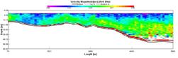
Figure 11: ADCP data files for Callista
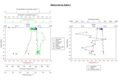
Figure 12: Station 1 vertical profile
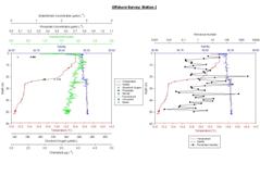
Figure 13: Station 2 vertical profile
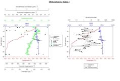
Figure 14: Station 3 vertical profile
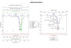
Figure 15: Station 4 vertical profile
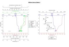
Figure 16: Station 5 vertical profile
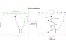
Figure 17: Station 6 vertical profile
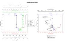
Figure 18: Station 7 vertical profile
|
|
The final transect
between Falmouth Docks and Carrick Roads showed an area of
high surface velocity (0.31-0.4ms-1 on the
outside of the meander at Carrick Roads, beginning
approximately 1500m along the transect. This is due to
current acceleration around the meander, which may be caused
by surface wind stress funneling through the channel, as
well as the start of the flood tide. There is no
correlation between this area and the backscatter profile.
Over the shelf, backscatter values are high (78-88dB) to
depths of 4-5m. This may be due to zooplankton populations,
vessels in Falmouth Docks or wave action.
Vertical Profile Data
The data explained here
groups different CTD stations in similar locations. Although
the ADCP does not indicate a front, data from other groups
has indicated a front present in the region shown in the
ADCP data and the vertical profile data works on the basis
that a front may have been present although rough weather
makes this difficult to verify. The analysis looks at both
temporal and spatial scales.
Stations 1-3 (Figures 12-14)
Physics
A loosely defined elongated front was located approximately
2 nm offshore at Station 2. On the landward side of the
“front” (Station 1) a slight thermocline was found at 8
metres with a temperature change of 0.3°C change. Due to
the shallowness of the estuary at this point the water
column is more mixed than further out in deeper water due to
shear stress. This is shown with the Richardson number
which at many points is below 0.25. (A Richardson number
of below 0.25 means the water column is more likely to
overturn and vertical mixing is greater.)
Further offshore the thermocline becomes more pronounced.
At Station 2, which is within the front, there is a
thermocline at 25 m depth with a change in temperature of a
degree. The Richardson number has a value of 2860.27 at the
thermocline showing very laminar flow and stable conditions
at this depth.
Station 3 has what appears to be two thermoclines and is
situated in what is typically considered to be stratified
waters. However, due to the high winds and low irradiance
over the days preceding our survey this stratification was
weakened. This is shown in the Richardson number which is
lower than Station 2.
Salinity is essentially constant with depth at all 3
stations with only minor fluctuations due to salt spiking
when there is a rapid change in temperature.
Chemistry
Nutrients are heavily affected by the amount of
stratification in the water column. Stratification prevents
mixing and so can lead to depleted nutrient levels in
surface waters as the supply is not replenished by nutrient
rich water being mixed up from below. Both Station 1 and 2
show lower concentrations of nitrate, phosphate and silicate
in the surface waters compared to the concentrations found
below the thermocline. However the change at station 1 is
negligible with depth which is consistent with its well mixed
profile.
Station 3 situated 3 nm offshore, displays an erratic plot
for both silicate and phosphate which, without risking data
aliasing, is difficult to analyse. For phosphate this
profile may reflect lab processing problems. Silicate shows
an association with chlorophyll and is most depleted at 8 m
where concentrations are highest and most abundant at 54 m. For dissolved
oxygen the concentration declines with depth, with a faster
decline occurring through the chlorophyll peak between 9 and
14 m. Nitrate shows a low concentration of 0.3 µMolL-1
which increases at the base of the thermocline/ chlorophyll
maximum. At the base of the water column Nitrate reaches 3.5
µMolL-1 at 54 metres.
Biology
The
fluorescence and discreet chlorophyll values correlate well.
At all three stations the biology is closely related to the
physical conditions. Station 1 shows a bulge in fluorescence
at 6 metres with high values throughout due to the well
mixed nature of the water column (see at the front >
physics). Station 2 shows a sharp fluorescence peak at the
base of the thermocline just below the maximum Ri number
(2860 at 19.6 m). This is a product of nutrients being
unable to mix into the surface layer due to lamination and
is typical of offshore and frontal summer production
patterns. Station 3 shows what could be considered an
atypical offshore profile.
Black Rock (Figure 15)
Physics
Between station 1 and 4 there is a 2.5 hour difference in
time. The tide during this period was a spring ebb with a
southern heading. A subtle decline in salinity is seen, as
is a rise in temperature. This is consistent with the ebbing
tide as the conditions within the estuary are warmer and
fresher (see estuary section). The Ri data shows that
between station 1 and station 4 the number of points above
1, indicating that the water column is more stable,
increases. This is probably due to the slower tidal flow
with progression of the tidal cycle
Chemistry
The nitrate levels at station 1 where higher throughout the
water column compared to station 4. The Phosphate levels
earlier in the ebb flow where at low but detectable
concentrations whereas when station 4 was sampled the
Phosphate was below detection levels, this is likely due to
dissolved phosphates acting as a limiting nutrient in
freshwater. Silicate is higher at station 4 when there is a
higher freshwater fraction because silicate is highest in
riverine waters. The phytoplankton data (see Figure 23) also
suggests that at station 1 a high number of euryhaline
diatom species maybe responsible for utilising the
silicate. Dissolved oxygen changes where negligible,
remaining within 10 µMol L-1 of 270 µMol L-1
at both depth and surface.
Biology
The biology earlier in the ebb flow was distributed
unevenly, with a broad peak of around 2.66 volts at 7 m and
depletion at the surface. The peak coincides with a high Ri
number suggesting that the chlorophyll build up at this
depth is associated with its relative stablility. Later in
the ebb the chlorophyll level becomes uniform with depth.
Discrete chlorophyll increases with the ebb with higher
levels at surface
Carrick Roads (Figures 16-18)
Physics
Station 5, 6 and 7 are taken half an hour apart starting
half an hour after low tide. Salinity increases as the tide
floods as the influence of salt water increases. Haloclines
coincide with the thermoclines on all 3 profiles. Though
the profiles were all taken after low tide, the Richardson
data shows turbulent flow above the thermocline at Station
5, more stable conditions at Station 6 and turbulent flow at
Station 7. This suggests that Station 6 shows slack water
conditions and Station 5 and 7 are ebbing and flooding
respectively.
Chemistry
The phosphate concentration shows 0 µMol L-1
though this may mean that the concentrations are below
detection levels or due to method errors in the lab.
Nitrate concentrations decrease with depth and also are
lower at Station 7 than Station 5. Silicate concentrations
are higher in surface waters which coincides with higher
fluorescence and chlorophyll concentrations. Due to method
errors in the lab, the surface dissolved oxygen
concentration is missing though the concentrations decrease
with depth at Station 5.
Biology
The highest fluorescence levels are found at the thermocline
where nutrients are being mixed up from below. Chlorophyll
is at higher concentrations at the surface and the
concentrations decrease by 0.5 µg L-1 between
Station 5 and Station 7.
Secchi disk data (Table 2) shows that for the samples
taken in the estuary, Sample Numbers 5-7, there is a deeper euphotic zone that at some of the offshore sites. This may
be due to the rough offshore conditions which would have
impacted the mixing and as such increased the turbulence in
the water. Also, when sampling the estuary, the tide was
flooding meaning that large amounts of river sediment were
not flowing seaward possibly reducing turbidity in our
sampling area.
| CTD Sample Number |
1 |
2 |
3 |
4 |
5 |
6 |
7 |
| Attenuation Coefficient (k) |
0.288 |
0.169 |
0.262 |
0.300 |
0.411 |
0.121 |
0.115 |
| Depth of Euphotic Zone (m) |
15.0 |
25.5 |
16.5 |
14.4 |
10.5 |
35.7 |
37.5 |
Table 2: Secchi Disk results showing depth
of euphotic zone as 3x secchi disk depth and the attenuation
coefficient (k)
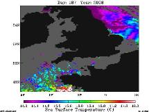
These two images illustrate the time series of sea surface
temperature for the days surrounding the sampling of
Callista, these are included to help explain the data
analysed above.
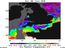
01/07/08
05/07/08
The satellite image on the left from the
1st July displays a front very close to the
southwest coast of Cornwall caused by heating of the surface
layer causing thermal stratification. By the 5th
July, when we collected offshore data, high winds and cloud
cover from the southwest had broken down the stratification
and produced a more mixed water column. On the right hand
plot you can clearly observe the reduced sea surface
temperature between the cloud covered areas.
Back to
Offshore
Back to Top |
|
BIOLOGY OF THE ESTUARY AND THE OFFSHORE AREA
In order to fully examine the patterns shown by the Biology,
both the data from the Estuarine sampling on Bill Conway and
the Offshore/Estuary sampling on Callista have been
collaborated to provide an overall picture of the water
column.
Phytoplankton
13 phytoplankton
samples were collected from Malpas to 3 miles offshore. Up
the estuary, the dominant phytoplankton found were
dinoflagellates (Figure 20), indicating the water was
stratified and nutrient poor conditions were present. Near
the mouth of the estuary diatoms became dominant, suggesting
mixing, and the total number of phytoplankton increased.
Then as samples were taken in the offshore region, dinoflagellates were found to be the abundant group of
phytoplankton showing the water became stratified again
(Figure 23).
The water
surrounding Black Rock had the highest abundance of
phytoplankton as it was estimated to be 600 phytoplankton
cells/ml. The lowest value (25 cells/ml) was found at the
riverine end of the survey, Malpas. In the vertical profile
the surface samples of every station had the most
phytoplankton as they received the most light.
Looking at
phytoplankton species in detail, the dinoflagellate
Alexandrium, a common, toxic coastal species, is
dominant at most stations that are dominated by
Dinoflagellates (Figures 19 and 24). Where diatoms dominate, the
dominant species is often Rhizosolenia setigera.
Zooplankton
Zooplankton samples were collected at 7
stations ranging from Smuggler’s Cottage to 3 miles
offshore. The zooplankton abundance is correlated to the
phytoplankton abundance as the zooplankton feed on
phytoplankton. Therefore, the zooplankton abundance follows
the same trend as the phytoplankton abundance. A total of 19
different classes of zooplankton were found in the entire
survey range (Figures 21 and 22). As expected, Copepods were
the most abundant at the majority of the stations. Only one
station had another dominant zooplankton and that was the
offshore station 5 where gastropod larvae were found to be
the dominant zooplankton. This could be due to breeding of
gastropods occurring in that area.
The copepods are expected to be
abundant as they are the largest source of protein in the
oceans. The most copepods (98,730 copepods/m3)
were found in the surface waters (7m deep) surrounding Black
Rock. This correlates with the chlorophyll concentration as
that too was highest in the Black Rock waters. Thus
confirming the zooplankton is most abundant at this location
because its food source, in the form of phytoplankton, is
most abundant. Offshore, the hydromedusae were more abundant
than inshore (Figure 22), whereas the opposite trend was
seen for Siphonophores and Cirrepedia larvae.
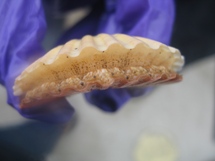
Figure 17
illustrates examples of some of the main zooplankton classes
found from our survey.
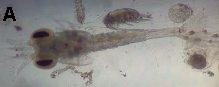 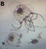 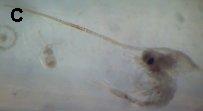
Figure 17: Zooplankton Samples (A) Fish
Larvae, (B) Hydromedusae, (C) Decapod Larvae
Back to
Estuaries
Back to Offshore
Back to top |
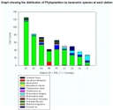
Figure 19: Estuarine Phytoplankton Species
Data (RIB and Conway)
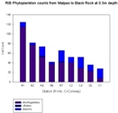
Figure 20: Estuarine Phytoplankton Taxa Data
(RIB)
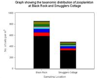
Figure 21: Estuarine Zooplankton Group Data
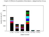
Figure 22: Offshore Zooplankton Group Data
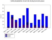
Figure 23: Offshore Phytoplankton
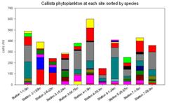
Figure 24: Offshore Phytoplankton Species Data |
WORKING WITH GEOPHYSICS
| Aims
On 8th July 2008, Group 3 used RV Xplorer to undertake a
geophysics survey of the Helford River area using Side-Scan
Sonar and Grab samples.
The aims of this investigation are:
-
To survey the benthic habitat around the
Helford River area to show main seabed types and geophysical
features
-
To determine how these features are
influencing the benthic biology via grab samples at certain
locations
-
Take video footage of transect area to compare
scan features to virtual images
Method
RV Explorer was used in conjunction with a towed side-scan
sonar to produce a benthic habitat map of the lower Helford
River area from five transects. After the side-scan sonar
was conducted areas of interest were examined in more detail
by taking grab samples using a Van Veen grab. These were
further investigated for biological interest on deck via
sieving using 2mm and 1mm mesh sieves. Photos were taken of
each grab sample for later identification and key species
noted. Video footage was initially taken across the five
side-scan transects and more detailed footage was taken at
each grab site.

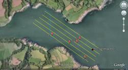
Figure 25: Printed Side-Scan sonar plot
Figure 26: Map of transect line with grab sites and video
transect
Transect Data for Side-Scan Sonar
|
Transect |
Latitude |
Longitude |
Time
(GMT) |
| Start |
Finish |
| 1 |
50°
06.139
50°
05.626 |
005°
06.610
005°
05.474 |
09:42:11 |
09:52:17 |
| 2 |
50° 05.582
50° 06.091 |
005° 05.527
005° 06.662 |
09:55:25 |
10:07:24 |
| 3 |
50° 06.054
50° 05.552 |
005° 06.715
005° 05.603 |
10:10:40 |
10:20:40 |
| 4 |
50° 05.499
50° 06.025 |
005° 05.622
005° 06.803 |
10:23:52 |
10:36:30 |
| 5 |
50° 05.984
50° 05.488 |
005° 06.842
005° 05.752 |
10:38:35 |
10:48:16 |
Back to
Geophysics
|
|
Results/Discussion
From the side-scan sonar profiles several areas of different
bed types were identified. These areas are shown in Figure
27
and help to indicate the different benthic habitats, data
which is then supported by the biological evidence from the
grab
samples.
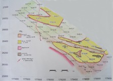
Figure 27: Seabed classification map from side-scan data
Our work on board Xplorer within
the Helford estuary allowed us to produce a seabed
classification map, displaying clear boundaries between
different sediment types. The dominant sediment types are
gravel, shingle and coarse sand, with bars of fine sand and
silt running through them, predominantly at the mouth.
These bars are most likely formed by the process of sediment
transport by river flow.
The dynamics of the river flow are causing deposition in
this zone, which is most likely to be due to a combination
of tidal influences and recent storm activity. A long term
ADCP and surveying stations would be needed in order to
completely determine the causes of the location and
orientation of the sand bars.
There is also a large sand bar by Porthallack, which is a
slightly sheltered location. This may cause a reduction in
current velocities, which would result in deposition of the
suspended sediments and the formation of the sand bar.
The sidescan sonar showed a large dark area across much of
the sample area. When the video transects and grabs were
employed, it was revealed that this dark area is an area of
graded boundaries containing more than one sediment type.
The bedrock on the right bank is at the edge of the headland
‘The Gew’. This is a very shallow location, which is why
the sidescan sonar was able to pick it up. On the sidescan
trace, this is displayed as a very dark area, as it is a
hard substance.
Video Analysis
Most of the grab samples focused to the South East of the
studied area. A video transect was taken in the North West
as well as each station to compare the side-scan profiles
and the grabs with what the actual sediment type is like.
The video recorded shingle sediment and dense seagrass at
transect 1. Greater diversity of biology including large sea
stars, invertebrates and juvenile fish. Midway between
transect 1 and 2 seagrass becomes less dominant on the sea
floor and shingle interspersed with bedrock forms the main
sediment type. The sediment type under transect 2 is mainly
shingle and sand with sparsely distributed shell fragments.
There is evidence of burrowing by infauna. Midway between
transect 3 and 4, the seafloor becomes very dense with shell
fragments, interspersed with bedrock and associated kelp.
Transect 4 onwards begins to become a less dense
distribution of shell fragments. The evidence from the video
correlated well with those from the side-san and grab
samples; isolating areas where sand, gravel and shingle were
dominant as well as shell fragments. The species present did
not show a great deal of correlation between sampling
methods, though this is due to a lack of live samples
retained in the grabs as well as seen on video.
As seen on Figure 29, a wreck was found on
transect 2, the wreck of The Rock Island Bridge.
The wreck measures approx 12m in length and was 10-12m deep.
This steamship sunk in 1920, and came to rest on the bottom.
After salvage attempts were abandoned, the ship was
flattened by explosives to maintain the channel.
Heavy deposition rates from the river have led to silt
covering the majority of the wreck.
By
measuring the lighter shadow down the long axis of the wreck
we find this feature to be 11.1m long and 0.5m high. This
correlates with photos and evidence from previous commercial
and recreational dives, which show metal hull ribs
protruding from the sand (Figure 28 files).
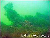
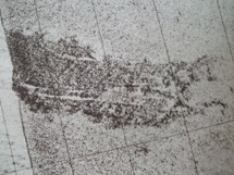
Figure 28: Photograph of The Rock Island Bridge
Figure 29: Side-scan sonar image of The Rock Island Bridge |
Sediment Data from Grab SamplesGrab 1
The sediment here was determined to be Bioclastic, made
up of mainly broken shell fragments that led to the
sediments being coarse and gravel like. This has allowed
sessile organisms to dominate as was seen from the biology
obtained from the grab sample (see below).
Grab 2
Video footage showed evidence of Arenicola burrows,
however no live samples were found in the grab. The sediment
type was fine sand with an average grain size of 187µm
or 2.5 phi, there were no obvious geophysical
features. This type of sediment would support burrowing
infauna as opposed to sessile fauna.
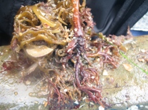
Grab 3
The video footage showed dense kelp populations which
would provide shelter and protection for juvenile fish and
other larvae. A sand eel was found in the grab supporting
this area as a protective site for fish. Many different
seaweed species were seen here, including Ulva lactuca
and the species Marthasterias glascialis. The
sediment type showed coarse sand and shingle with broken
shell fragment, the average grain size was 2000µm
or -1 phi.
Grab 4
Video footage again showed dense kelp populations as for
Grab 3. The sediment was also of a similar type, coarse sand
and shingle with broken shell fragments, the average grain
size here was 750µm or 0.5 phi.
Grab 5
As in Grab 2, Arenicola burrows were identified from the
video footage. The sediment was seen to be well sorted
medium sand with an average grain size of 375µm.
Only infauna were found here as the sediment type indicates
an area unsuited to epifaunal species. |
Video Grab 2
Video Grab 3
Video Grab 4
Video Grab 5
|
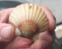
Biology Obtained from Grab Samples41) 50°
05.815 N, 005° 06.459 W
Class Bivalvia
Aequipecten
opercularis
Queen Scallop
·
Shell up to 9cm long with ~20 radiating ridges and corrugated
grooves.
·
Young
attached to substrate by byssus threads, adults can swim
by ‘flapping’ shell
·
Occurs
commonly off British coasts on coarse gravel and
sandy sediments.
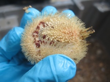
2) 50°
05.721 N, 005° 05.966 W
Class Echinoidea
Echinocardium
cordatum
·
Thin heart
shaped test with dense covering of yellow spines.
·
Lives
buried in sand, 10-20 cm deep. Feeds by extending long
tube feet of abulacral plate to the surface through a hole.
·
Common
around all coasts of Britain.
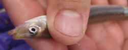
Class
Osteichthyes
Ammodytes
tobianus
Sand Eel
·
Long,
slender eel like fish, silvery/sandy coloured
·
Belly
scales arranged in chevrons, simple lateral
·
Very
common around all British coastline. Occurs from intertidal
down to about 30m
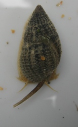
3) 50°
05.524 N, 005° 05.814 W
Class Gastropoda
Hinia reticulate
Netted dog-whelk
·
Brown
shell, up to 3cm tall, fat and conical with about 7 poorly
defined whorls.
·
Predator
of other small invertebrates
·
Widespread
around Britain. Found in muddy sand or gravely
sediments from the lower shore and shallow litoral zones.
Class Polychaeta
Lanice conchilega
Sand mason
(tubes only, in
sediment)
·
Up to 30cm
long, head with numerous white or cream tentacles,
three pairs of blood red, branched gills behind head.
·
Tube
constructed from coarse sand grains, shell and stone
fragments.
·
Found mid
shore downwards around all of Britain.
Back to Geophysics
Back to top |
 |
GENERAL
CONCLUSIONS
|
We completed
biological, chemical, physical and geophysical surveys of
the Fal estuary and surrounding offshore areas between 1st
July and 8th July 2008.
During the summer period, one would expect to see an
increase in thermal stratification of the water column
coupled with the occurrence of an offshore frontal system,
where warmer more stratified seawater meets a cooler
estuarine water body. The ADCP data from our offshore survey
did not indicate the presence of a significant frontal
system (Figure 11) although this has been put down to rough
weather conditions. The vertical profiles further indicated
the presence of stratification, with Figures 12-14 showing
how the patterns changed across the theoretical position of
the front. As expected we found more stratified waters where
the front had previously been found, with a strong
thermocline typified by chlorophyll maximum and increasing
numbers of dinoflagellates (Figure 23). The estuary itself
was seen to be more well mixed, as would be expected
(Figures 1-6) and there was a clear transition from well
mixed to partially mixed with progression landward as would
be expected in an estuarine environment.
During our sampling
time, issues such as bad weather conditions, especially in
the offshore environment, arose. During the seven days that
we were sampling, the Fal area received more than the
monthly average of precipitation for the Cornwall area.
This obviously led to increased surface runoff and river
input, along with strong winds that broke down the frontal
system found earlier in the week. The increased
precipitation may explain the addition of phosphate within
the estuarine system (Figure 10), other nutrient values
within the estuary were found to be conservative (Figures 8
and 9) indicating a balance between addition and removal,
most likely through biological activity (Figure 19).
The data from estuary and offshore was complemented by that
of the geophysics survey which indicated the seabed types
and enabled us to look more closely at the benthic ecology
and their associated habitats (see Working with Geophysics).
The data collected over the survey period enabled our group
to gain an understanding of the change in physical, chemical
and biological processes and activity with progression from
the head of the estuary to offshore. We have been able to
correlate results to show how alterations to physical and
chemical parameters have affected the biology of the water
column from nutrient and current pattern changes to the
affect of various geophysical bed forms.
Back to top
|
REFERENCES
| 1.
www.projects.ex.ac.uk/geomincentre/estuary/Main/loc.htm
2. Aminot, A., Belin, C., Chapelle, A., Guillaud, J., Joanny,
M., Lefebvre, A., Menesguen, A., Merceron, M., Piriou, J.,
Souchu, P. (2001) “Coastal Eutrophication: A review of the
situation along the French coasts” Archimer, Ifremer’s
Institutional Archive 22
3. Parsons, T.R., Maita, Y. and Lolli, C. (1984) A
Manual of chemical and biological methods for seawater
analysis. pp.173, Pergamon Press London.
4. Gibson, R., Hextall, B., and Rogers, A. (2001)
Photographic guide to the sea and shore life of Britain and
North-West Europe. Oxford Press, Oxford.
5. Grassoff K., Kremling, K., and Enrhardt, M. (1999)
Methods of seawater analysis, 3rd edn, Wiley - VCH
6. Johnson, K. and Petty, R.L., (1983).
"Determination of nitrite and nitrate in seawater by flow
injection analysis" Liminology and Oceanography,
28, pp.1260-1266
|
|
|