![]()
Falmouth 2008
Group 1
![]()
|
|
Falmouth 2008 Group 1 |
|
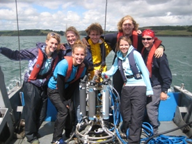
~ Andy Ashdown ~ Arwen Bargery ~ Alex Bryk ~ Joe Green ~ Doug March ~ Allison Martin ~ Marcus Sampson ~ Emily Savage ~ Emma Steventon ~ ~ Rosanna Von Zweigbergk ~
|
|
|
|
|
|
|
|
![]()
![]()
![]()
![]()
![]()
![]()
![]()
Field Course
|
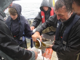
We are one out of nine groups of second year students from Southampton University who participated in a two week field course in Falmouth, from June 30th to July 11th, 2008. This field course was designed to investigate the physical, biological, and chemical characteristics of the Fal region in Cornwall. To accomplish this, three days of fieldwork were carried out measuring: offshore, estuarine and certain geophysical properties of the region. In-depth descriptions of these three days and the results they produced can be found in the sections following. Some of the major findings include a reverse ekman spiral found offshore and the significant effect of the sewage input on the biology of the estuarine waters. Beautiful pictures of the benthic habitat of the Fal Estuary, including unique maerl beds captured using underwater video technology new to this field course, can also be found on this website. Combining our findings with the eight other groups we were able to increase our understanding of the biogeochemical relationships and processes that are prevalent in this area. |
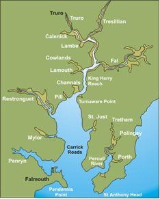
Falmouth Region
|
The area around the Fal has suffered from intense mining and shipping activities in the past. The tributaries running through areas that have had heavy geological interference from the Cornish metal and china mining industry, leaving the area with increased levels of iron, tin, zinc, copper and arsenic. Currently only copper exceeds the recommended levels (Langston et al, 2003). Tribultyl Tin (TBT) has also been found in high quantities in the area and although banned from use on all EU ships in 2003, was used as an anti-fowling paint on the hulls of boats which caused imposex in dog whelks and other marine organisms (Gibbs et al, 1987). A major recent pollution incident occurred in 1992, known as The Wheal Jane incident, when a disused Cassiterite mine was drained into the area. Other anthropogenic influences in the area are caused through local dredging, tourism and sewage outfall. In particular there is a sewage outfall at Black Rocks, which will cause increased levels of nitrates and phosphates in the area. The Fal Region has therefore been designated cSAC status and is a sensitive area (Eutrophic) under the Nitrates Directive 91/676/EC. (Langston et al, 2003). |
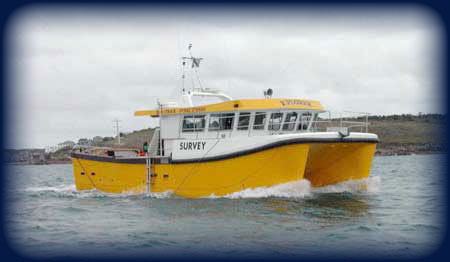
| RV Bill Conway | RV Xplorer |
|
|
|
|
The Bill Conway was used for our work in the estuary. 11.74 meters long purpose built research vessel
Simrad SDGPS |
The Xplorer was used for geophysical surveying with a fully equipped side scan sonar and grabs. 12m x 5.2m x 1.2m Gemini fastcat
Side Scan Sonar and Boomer. |
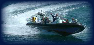
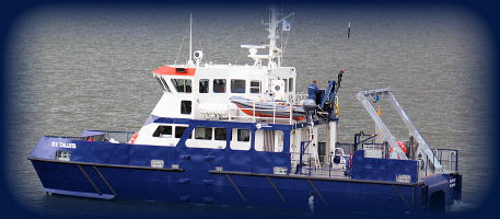
| RIB Ocean Adventure | RV Callista |
 |
 |
|
The RIB is a smaller and more versatile boat with little draft allowing it to be used to collect samples further up the estuary. Hull Ribtec 700 Simrad SDGPS, Depth sounder and Chartplotter |
The Callista is primarily an offshore research vessel with fully equipped wet and dry labs. 19.75 meters long twin hull purpose built research vessel
Hull mounted RDI Workhorse ADCP 600Khz “A” frame and associated winch – 4 tonne lifting capacity (Max vert height 3.5m approx) |
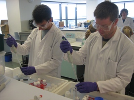
The following procedures for analysing chemical and biological samples were adopted in the offshore and estuary practicals.
|
Dissolved Oxygen Samples were obtained directly from the Niskin bottles on deck and contained in glass bottles. In accordance with the Winkler method (Head, 1985), 1ml of manganese sulfate solution and 1ml of alkaline potassium iodide were added to each sample. Care was taken to ensure that no air bubbles were contained in the bottles. Samples were then safely secured and stored under water for laboratory analysis the following day. Oxygen concentrations were determined in the lab by automated titration following the method outlined by Grasshoff et al, 1999. |
|
|
Phosphate Sample seawater was obtained from the Niskin bottles and stored in glass bottles for laboratory analysis the following day. Phosphate concentrations were determined using spectrophotometry following the method outlined by Parsons et al, (1984), yielding results with a detection point of 0.03 μM. |
Nitrate Samples for nitrate analysis were obtained from the Niskin bottles on deck and stored in glass bottles for later lab analysis. Nitrate concentrations were determined using a flow injection method detailed by Johnson & Petty, (1983), giving concentration values with a detection value of 0.1 μM. |
|
Chlorophyll 60ml of sample seawater were filtered through two replicate GFF filters and then placed in glass tubes containing 6ml of acetone and stored for chemical analysis in the lab. Chlorophyll concentrations were analysed using titration following the method outlined by Parsons et al, (1984). |
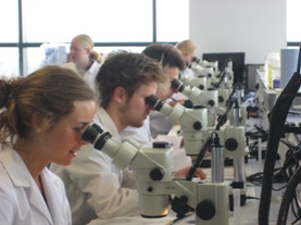
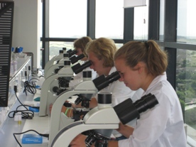
Zooplankton Zooplankton samples obtained from nets were analysed under 5x magnification using Motic SMZ-168 Series microscopes. Orders of organisms were identified with the help of taxonomic identification guides such as Haward et al, (1996). 5ml of sample water from each station was analysed under the microscope on Bogorov slides and a tally chart for each order was constructed, allowing for the zooplankton concentration per m3 to be calculated. |
|
Phytoplankton Seawater samples were concentrated x10 and 1ml from each station was analysed under the Motic SMZ-168 Series microscopes. Species of phytoplankton were identified and counted on Sedgewick Rafter chambers. |
Dissolved Silicon Silicon samples were stored in plastic bottles for lab analysis. Silicon concentrations were determined using spectrophotometry as outlined by Parsons et al, (1984), giving results with detection points of 0.3 μM. |
![]()
|
|
|
 |
Date: 1st July 2008
Principal Scientific Officer: Emily Savage
|
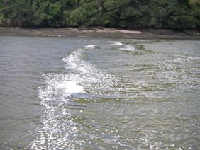
Introduction On the 1st July 2008, the RV Callista was taken out into the offshore region beyond the waters of the Fal estuary. The aim of the day was to measure various biological, chemical and physical parameters of the water column to enable a tidal mixing front to be located and characterised. A front is defined as a transition zone between two distinct bodies of water and should be present at this time of year between the well mixed and the stratified waters. The well mixed waters are found at the mouth of the estuary where they encounter the sea and the stratified waters are consequently found offshore where solar warming of the surface layers is great enough to overcome mixing processes and enable the water column to stratify. |
|
Tides
|
Station Locations
|
|
Aim
|
Equipment
|
|
Crew: PSO: Emily Savage Computer Master: Alex Bryk Computer Analyst: Allison Martin, Alex Bryk, Andy Ashdown Chemists: Rosanna Von Zweigbergk, Arwen Bargery, Emma Steventon, Allison Martin, Equipment Deployment: Doug March, Andy Ashdown, Joe Green Secchi Disk: Marcus Sampson Logbook: Allison Martin |
|
|
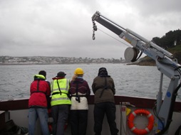
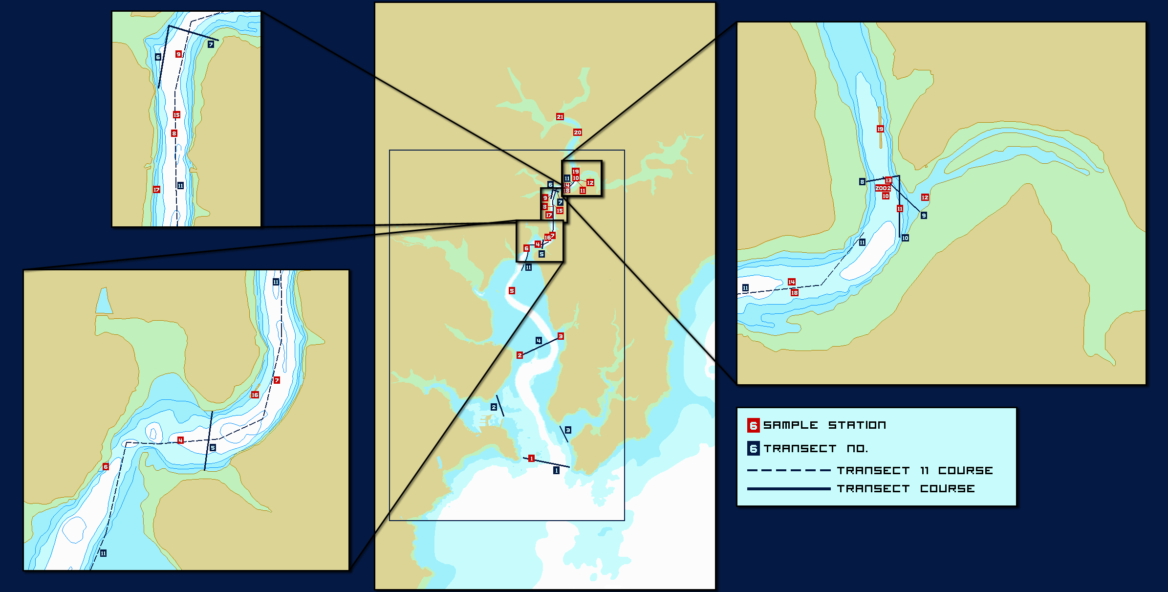
Method A total of 7 stations were sampled on a route from Falmouth Docks reaching 7 nautical miles offshore (please see route map). During the planning stages beforehand it was decided that a number of stations would be sampled at set distances, but that a degree of flexibility was required in order to adjust to what we discovered at the first few stations. Our initial plan was to determine the location for sampling stations in regard to changes in temperature monitored by the thermosalinograph. However, because the thermosalinograph did not work correctly on that day, we altered our plans and dropped the CTD scan at the various locations to gain information on the temperature profiles of the water column. Depending on the readings, we altered our route in search of the front. We also activated the ADCP when we suspected to be near the front. By interpreting the backscatter from the ADCP we could identify potential frontal systems. Once a consensually good station was located the CTD was deployed with the Niskin bottles primed in order to collect samples, the idea being that a profile would be taken on the way down and samples would be collected on the recovery. Roughly, the aim was to take one sample at depth, one at the thermocline/chlorophyll maximum and one at the surface. At the same time a secchi disk was deployed off of the front of the vessel. Following the recovery of the CTD a vertical closing net was deployed and closed at two depths deemed appropriate after examining the CTD profile. Again, the aim was to roughly have one above and one below the thermocline. Meanwhile the Niskin bottles were decanted into two further containers – a small glass bottle for later O2 analysis and a large plastic container that would later be divided up in the wet lab for Fluorometer and Nutrient analysis. |
|
The CTD was used to obtain measurements of temperature, oxygen saturation, chlorophyll concentration, and water samples used for nitrate, phosphate and silicon analysis. Salinity was measured with the CTD though not plotted as the water column offshore is homogenous due to the little fresh water input seen in this system.
|
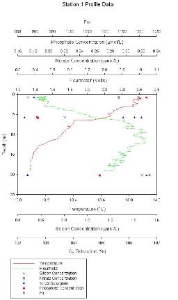
Figure 1.1: Station 1 CTD and lab results graph (click to enlarge) |
Station 1 At station 1 (figure 1.1) chlorophyll is lowest at surface, reaching a maximum of ~2.7µmol/L between 8 and 12m. The thermocline occurs between 5.5 and 7m with a temperature difference of 0.3°C. Oxygen saturation is lowest either side of the chlorophyll maximum; at the surface and again at 20m. Close to the chlorophyll maximum at 5.5m oxygen saturation is ~106.5%, above and below the chlorophyll maximum the O2 saturation is approximately 102.5%. Nitrate and phosphate reach their lowest values at around 5.8m, Nitrate concentrations range from ~0.42-1.05µmol/l, Phosphate concentrations range from ~0.185-0.323µmol/l. Silicon appears to increase with depth from 0.5 at the surface to 1.5µmol/l at 20m. |
|
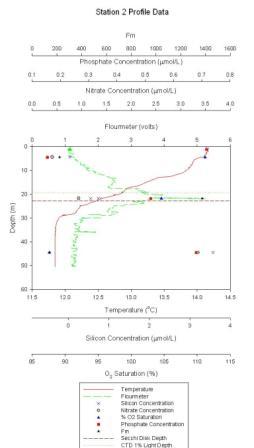
Figure 1.2: Station 2 CTD and lab results graph (click to enlarge) |
Station 2 At station 2 (figure 1.2) chlorophyll shows a sharp peak at 22m of ~5.3µmol/L. A thermocline is present from 12 to 25m, covering a temperature range of 1.5ºC. There appears to be a general decrease in O2 saturation from 112-87.5% between the surface and 45m. Nitrate values range from 0.4 at the surface to 3.3µmol/l at 45m. Phosphate decreases from 0.15 at the surface to 0.68µmol/l at 45m. Silicon increases from trace levels up to a maximum of 3.6µmol/l at depth. |
|
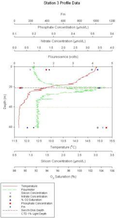
Figure 1.3: Station 3 CTD and lab results graph (click to enlarge) |
Station 3 At station 3 (figure 1.3) maximum chlorophyll concentration of 4.7µmol/l occurs at ~21m. The thermocline occurs between 18 and 25m with a temperature range of 2ºC. O2 saturation appears to be greatest in the first 20m, 103%, and lowest, 90%, at 60m. Nitrate values are at a minimum at 21m, 0.4µmol/l, and greatest above and below the thermocline at ~3.4µmol/l. Phosphate values are also at a minimum at 21m, 0.15µmol/l, above and below the chlorophyll maximum phosphate concentrations are greater at ~0.55µmol/l. Silicon concentrations are ~0.75µmol/l in the surface 25m and at 60m, silicon concentrations are greater at 3.25µmol/l.
|
|
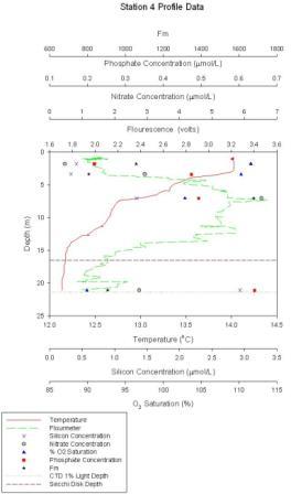
Figure 1.4: Station 4 CTD and lab results graphs (click to enlarge) |
Station 4 At station 4 (figure 1.4) a clear thermocline with temperature difference of approx.2.6˚C. Chlorophyll is distributed largely over a large depth of the water column, reaching a maximum of 3.5 volts. Surface chlorophyll concs. reach around 2.1volts. Nitrate concentration is highest mid depth around 7m, corresponding to the chlorophyll maximum peak. Phosphate and silicate increase with depth. Oxygen saturation decreases with depth, with maximum surface values of ~112%. The 1% light intensity is at ~22m depth.
|
|
Figure 1.5: Station 7 CTD and lab results graphs (click to enlarge) |
Station 7 At station 7 (figure 1.5) the chlorophyll maximum occurs at ~10m and at a concentration 3.45µmol/l. The thermocline is from 5-12m and covers a range of 1.3ºC. O2 saturation decreases with depth, from a maximum of 117% near the surface to a lowest recorded value 93% at 25m. Nitrate concentrations range from a minimum of 0.6µmol/l at 10m to ~2.0µmol/l above and below the chlorophyll maximum. Phosphate increases with depth from 0.17µmol/l at the surface to 0.38µmol/l at 25m. Silicon concentrations also increase with depth from 0.36µmol/l at the surface to 2µmol/l at 25m.
|
Water Column Chemical and Physical Properties Discussion
|
From the CTD profile data graphs many aspects of the frontal system can be seen. The stations show progressively more thermal stratification from inshore to offshore. Station 7, on the front, has the largest surface chlorophyll concentration, with the fluorometer reading 2.4 Volts. This increased surface chlorophyll concentration may be due to convergence of flow “by concentrating the biomass from the mixed and stratified water on either side” (Sharples & Simpson, 2001). Overall chlorophyll concentrations of the water column are greatest at the stations close to the front (2, 4 and 7), also the chlorophyll maximum becomes progressively more defined offshore. Oxygen saturation is noticeably greater at the front (station 7) at 117% compared to 105% in the well mixed waters (Station 1) and 103% in the stratified offshore water of station 3. This may be a direct result of the increased primary productivity at the front. Further explanations for increased oxygen levels could be explained by entrainment from the enhanced wave breaking which occurs at fronts and their interaction with currents. Such conditions increase the generation of gas bubbles and associated downwelling currents create higher oxygen levels further down the water column (Baschek et al, 2006). |
![]()
|
Figure 1.6: Zooplankton graphs key
Figure 1.13: Total zooplankton per m3 at each station |
Figure 1.7: Staiton 1 depth 4-10 m zooplankton Graph |
Figure 1.8: Station 2 depth 25-20 m zooplankton graph |
Figure 1.9: Station 2 depth 21-0 m zooplankton graph |
|||||||||||||||||
|
Figure 1.10: Station 3 Depth 28-0 m zooplankton graph |
Figure 1.11: Station 3 depth 15-0 m zooplankton graph |
Figure 1.12: Station 4 depth 15-0 zooplankton graph |
||||||||||||||||||
|
Figure 1.14: Station 4 depth 3-0 zooplankton graph |
Figure 1.15: Bongo Nets at Station 7 zooplankton graph |
|||||||||||||||||||
Zooplankton Results
|
As seen in figures 1.7-1.15 copepods were the dominant group at every station and depth sampled, with the highest densities being 46250 per m3 at depths between 0-15m at station 4. Copepod nauplii were also abundant at all stations except between 15-0m at station 3, with a maximum of 1450 per m3 found at station 2 between 21-0m. The Siphonophores, which were most abundant at Station 1, were found in greater concentration in the shallow water (above 20m) but at all stations other than station 1 and station 2 at 25-20m, the Hydromedusae exceeded the Siphonophore densities. Bongo nets were deployed in the surface and showed a taxonomic distribution of zooplankton similar to that of stations 1 and 2, with the groups of highest concentration being the Copepoda, Hydromedusae and Siphonophores. The highest densities of zooplankton were found at station 2 between depths of 25 and 20m and the lowest at station 3 between 28 and 0m. At all stations, the zooplankton were distributed in the region of water surrounding the chlorophyll maximum and the thermocline. |
| Station | Simpsons diversity index |
Through calculation of a Simpsons Diversity index for each of stations 1 to 4, it can be seen that station 4 represented both the highest and the lowest diversity with the highest (of 0.85) being the shallower of the two samples. Overall, the zooplankton diversity was greatest in the samples taken from the shallower water for each site. The likely explanation for this is the greater level of irradiance supporting phytoplankton growth in the shallower water, therefore providing an grazing source for the zooplankton. |
| 1 (4-10m) | 0.48 | |
| 2(25-20m) | 0.68 | |
| 3(28-0m) | 0.68 | |
| 1 (4-10m) | 0.8 | |
| 2 (21-0m) | 0.83 | |
| 3 (15-0m) | 0.83 | |
| 4(3-0m) | 0.85 |
Zooplankton Discussion
|
Zooplankton graze at and around the chlorophyll maximum where phytoplankton concentrations are highest. Due to the seasonal succession of phytoplankton in temperate waters, the nutrient depleted surface water that is apparent during the summer has resulted in the deepening of the chlorophyll maximum. Henceforth, the zooplankton migrate to the deeper waters around the thermocline and chlorophyll maximum where light levels are still sufficient but nutrient concentrations are higher due to mixing from below (Colebrook, 1979). |
![]()
|
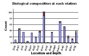
Figure 1.16: Biological composition at each station graph 9Click to enlarge)
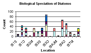
Figure 1.17: Biological speciation of diatom graph (click to enlarge)
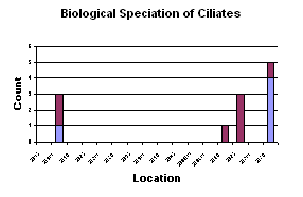
Figure 1. 18: Biological speciation of ciliates graph (click to enlarge)
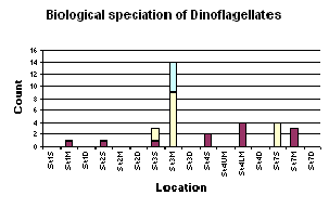
Figure 1.19 Biological speciation of dinoflagellates graph (click to enlarge) |
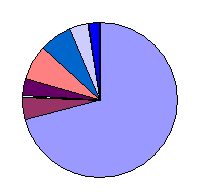
There is the general compositional trend in the offshore region of high dominance by diatoms over dinoflagellates and ciliates. (Figure 1.16) Dinoflagellates are present in low numbers at most of the sites and ciliates only appear at the more inshore, less stratified sites (station 1 and 7). The obvious reasoning for this is the season. In sea temperature terms it is still relatively early in the summer i.e. the sea has not yet warmed enough to become significantly thermally stratified. This means that the water column is still fairly mixed and on top of this, recent bad weather has increased the mixing processes occurring. Mixing keeps the water temperature lower and the nutrient content of the water higher. These are ideal conditions for diatoms, which grow faster and tend to out-compete dinoflagellates, especially if the limiting nutrient of silica, is available for the diatoms to build their frustule. If the dinoflagellate numbers are looked at individually, the highest abundance of them can be witnessed at station 3 at the thermocline (21.2m). Station 3 was highly stratified and the thermocline at this location generally contained the most phytoplankton. The higher population of dinoflagellates at this site compared to other sites is due to the stratification. The lower level of mixing action at this site is more accommodating to dinoflagellates because they are motile and can move vertically through the water column, in and out of the nutrient rich waters around the thermocline. Diatoms on the other hand, are immobile so rely heavily on mixing to move them into the nutrient rich waters. At the more stratified sample sites (2 & 3) there is a more obvious increase in phytoplankton abundance from the surface waters to the thermocline. This is due to the nutrient mixing at stratified sites being restricted by the thermocline and thus fewer phytoplankton existing above it compared to within it, as long as the thermocline is still in the euphotic zone. Site 4 was situated two miles off shore and also has high phytoplankton abundance just below the thermocline. This site was not as well stratified as site 3 but did appear to experience a certain amount of upwelling. This was marked by a high nutrient level under the thermocline, which would explain the high phytoplankton population here. The diatom composition (Figure 1.17) was very mixed but the species that appeared most frequently were Rhizosolenia delicatula, Rhizosolenia setigera, Rhizosolenia alata. This composition will be comparable with the estuarine populations. |
![]()
|
Station 1 |
|
|
Magnitude |
Direction |
|
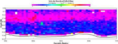
Magnitudes between 0 and 0.5m/s at this station (fig. 1.20). There is no differentiation between the top water layer and the bottom water layer. There are no visible patterns and this can be attributed to the fact that this data was taken at 09:38 (GMT), which was taken at slack water at 09:45 |
This data was collected at slack water, this means that no particular flow direction (fig. 1.21)should be found through out the water column. At the beginning of the sample a flow out of bay can be seen at almost 180o due south. flow direction throughout the remainder of the water column is sporadic and non-uniform. |
|
Figure 1.20: Station 1 ADCP Velocity Magnitude (click to enlarge) |
Figure 1.21: Station 1 ADCP Velocity Direction (click to enlarge) |
|
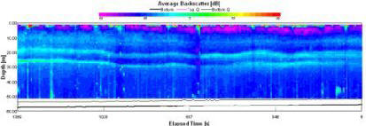
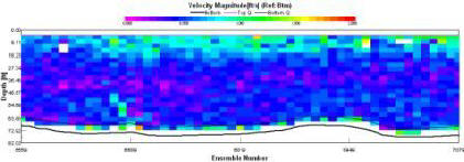
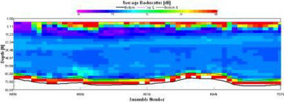
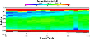
Backscatter |
|
High readings of backscatter (fig. 1.22) can be seen in the surface layer (93-125dB). Below the surface layer (>4.6m), progressive reduction in backscatter (60-76dB) can be observed, with patches of comparably very low backscatter (60dB). |
|
Figure 1.22: Station 1 ADCP Backscatter (click to enlarge) |
|
Station 2 |
|
| Magnitude | Direction |
|
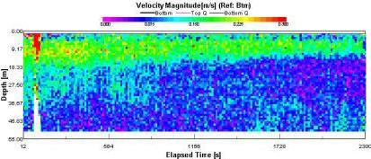
Varies between 0 and 0.3m/s down through the water column. Flow magnitude (fig. 1.22) is low in the upper layer of the water column (0.075-0.150m/s). There is a noticeable increase down into the water column, which peaks at between 20-30m (0.225-0.300m/s). After 30m the velocity decreases again down to the sea bed. |
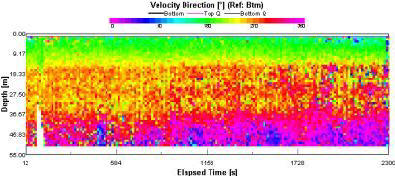
At the surface the flow was found at approximately 45o to the wind direction (fig. 1.23), which should be expected. This switches at roughly 10m and begins to flow towards the coast with the tide. This flow direction dominates on average for the rest of the water column. |
|
Figure 1.22: Station 2 ADCP Velocity Magnitude (click to enlarge) |
Figure 1.23: Station 2 ADCP Velocity Direction (click to enlarge) |
| Backscatter |
|
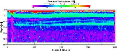
At the surface backscatter is high because of the surface turbulence (90-75dB). Below this an area of relatively low backscatter is obvious and this can probably be attributed to a shadow caused by the turbulence. The backscatter remains low down through the water column until roughly 20m. At this point there is an increase to 75dB, just above the thermocline. At the thermocline our data shows a chlorophyll peak, which might represent a high phytoplankton concentration. Below the thermocline another peak of roughly 75dB is found and then it remains low down to the sea floor. The peaks found at 20 and 25m are possibly caused by grazing zooplankton at high concentrations. |
|
Figure 1.24: Station 2 ADCP Backscatter (click to enlarge) |
|
Station 3 |
|
|
Magnitude |
Direction |
|
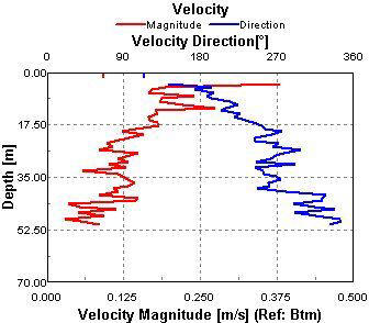
Velocity magnitudes (fig. 1.25) measured at sight 3 were, on average relatively low with a total range of 0 – 0.3m. Surface velocities measured at the site were found to be ~0.15m/s and penetrate to a depth of 18m. Velocity magnitude values measured below this depth are relatively low ranging between 0.05 and 0.1m/s. |
Flow direction values (fig. 1.26) found at site 3 show a 180 degree rotational change between surface and bottom water. Surface flow oriented at 180 degrees gradually changes with depth to a bottom water flow direction of near 0 degrees. Note this change is gradational and continues through the duration of the ADCP transect . A reverse ekman spiral can also been seen (see further discussion below). |
|
Figure 1.25: Station 3 ADCP Velocity Magnitude (click to enlarge) |
Figure 1.26: Station 3 ADCP Velocity Direction (click to enlarge) |
| Backscatter |
|
Station 3 exhibited backscatter values with a relatively low spectral range (From 65 to 80) (fig 1.27). Two distinct zones of relatively high backscatter values ranging between 71 and 73 were recorded at ~9m and ~21m straddling a thermocline of depth (17-20m). Backscatter readings below the 23 meters are uniformly low exhibiting values of less than 68. |
|
Figure 1.27: Station 3 ADCP Backscatter (click to enlarge) |
|
Station 4 |
|
|
Magnitude |
Direction |
|
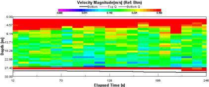
Overall velocity values are high for the area (fig. 1.28), between 0 and 2m/s. Surface velocity is highest (0.5 – 2m/s) and it decreases down through the water column. |
The direction found is in accordance with the flood tide as direction of flow is in towards Falmouth Bay (fig. 1.29). |
|
Figure 1.28: Station 4 ADCP Velocity Magnitude (click to enlarge) |
Figure 1.29: Station 4 ADCP Velocity Direction (click to enlarge) |
| Backscatter |
|
There is backscatter peaks (fig. 1.30) at the surface and at the sea bed, but no significant peaks throughout the water column. |
|
Figure 1.30: Station 4 ADCP Backscatter (click to enlarge) |
|
Station 7 |
|
|
Magnitude |
Direction |
|
Shows high velocity at the surface (above 0.3m/s), which rapidly decreases down to roughly 8 meters (fig. 1.31) At this point the water column stabilizes and the velocity remains the same (between 0.225 and 0.074 m/s) until it reaches just above the sea bed. At this point velocity increases to more than 0.3m/s. Note, that through the stable section of the water column the velocity does decrease on average, but only by a very small amount. |
Station 7 was taken at 14:52 (GMT) and high tide occurred at 15:31 (GMT), this means that the tide was going in. This corresponds with the flow shown on the velocity direction diagram (fig. 1.32) in that the flow occurred at between 360o and 90o, flowing through 0o and this corresponds to the tide flowing into the bay. |
|
Figure 1.31: Station 7 ADCP Velocity Magnitude (click to enlarge) |
Figure 1.32: Station 7 ADCP Velocity Direction (click to enlarge) |
| Backscatter |
|
Shows high backscatter at the surface layer and at the sea bed. Through the water column (fig. 1.33) a band of slightly higher backscatter rising up through the water column and presumably reaching the surface just off the read out. This can be used as an indicator for the front. |
|
Figure 1.33: Station 7 ADCP Backscatter (click to enlarge) |
|
At station 3 the ADCP data recorded showed a complete switch in direction down through the water column. Initially Ekman transport was proposed as the cause for this movement. However upon closer inspection we discovered that the net direction of transport was occurring in the opposite direction to that, that would have suggested wind driven Ekman transport. The readings were taken at 11:51 (GMT) on the 2nd July, 2008 and admiralty charts suggested high tide would be at 15:31 (GMT). This meant that flow direction would be expected at roughly 360o to the boat into Falmouth bay. However our surface data indicated that the rotational change through the water column was occurring in the opposite direction. We propose that this anomaly has been caused by a process called reverse Ekman transport. In contrast from a wind driven spiral, a reverse Ekman spiral originates from a bottom current flowing in a given direction. The orientation of friction associated with this flow is working in a direction 180 degrees from the original current track. As Coriolis is the mechanism for right sided deflection in the northern hemisphere, the bottom derived spiral will rotate accordingly. However, when viewed from the surface the direction of rotation appears to be left sided. Typical Ekman spirals display a diminishing flow velocity with distance from the originating force, in this case the north flowing bottom current. However, velocity magnitude data measured at the site reveal a pattern in opposition to this general trend (Aebecht et al., 1997). In this case surface velocities were measured at slightly higher magnitudes than those measured at depth. The occurrence of this trend can be attributed to a signal lag time between directional changes in bottom flow originating from tidal reversal. In addition, as a reverse ekman spiral initiates at the sea bed, wind conditions will have a relatively large influence on surface current dynamics and can potentially erase most of the Ekman influence. |
Richardson Number
|
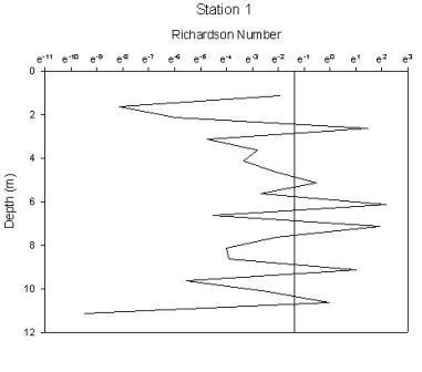
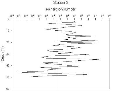
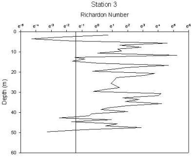
Figure 1.34: Station 1 Richardson number graph
Figure 1.35: Station 2 Richardson number graph
Figure 1.36: Station 3 Richardson number graph
|
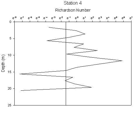
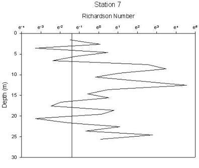
Station 1(figure 1.34) shows greatest stability in the region of the chlorophyll maximum. There are 2 regions of high instability, one at the surface and one at depth. The peak at the surface occurs at 1.6m and gives a Richardson’s value of 0.0002 and corresponds to where the chlorophyll concentration is lowest. The lowest Ri value observed from any station, therefore indicating greatest instability has a value of 7.5e005 at 20m and corresponds to the depths where water temperature and oxygen saturation are lowest. Stability of the water column at station 2 (figure 1.35) has increased from station 1. Instability increases at depths beyond 26m after which point the chlorophyll concentration declines rapidly, with Ri values ranging from 0.5 to 0.0007. The greatest instability again corresponds to the lowest oxygen saturation value. Station 3 (figure 1.36) is a very stable water column with the only depths showing instability being at 3m and between 42 and 49m. Both of these zones correlate to the lowest chlorophyll concentrations. Stable Richardson’s values range from 1.5 to 11.6 and the unstable from 0.1 to 0.01. Station 4 (figure 1.37) has 2 main areas of high instability which correspond to the areas of water surrounding the chlorophyll concentration boundaries. A high Richardson’s value of 333 (which is the highest value observed for any station) is seen at 11.6m is located at a depth equal to the region of the chlorophyll maximum. Station 7 (figure 1.38) has 2 peaks in stability at depths of 8.6m and 12.5m, with Richardson’s values of 32 and 94 respectively which correspond to the 2 levels of the thermocline that exist at this station and also the 2 levels of chlorophyll peaks. |
|
|
Figure 1.37: Station 4 Richardson number graph |
Figure 1.38: Station 7 Richardson number graph |
|
ADCP Discussion
|
The aim of our offshore work was to identify a tidal mixing frontal system. Salinity values were homogenous throughout the experiment showing no significant variation with depth and are thus not shown graphically. Our nearest inland location (station 1) near Black Rock exhibited a well mixed water column. Station 3, located 7 miles offshore displayed a highly stratified water column. These stations mark the geographical boundaries on our study. Between these two sites a gradational change from a well mixed water column to highly stratified water column was observed. Based on this observation station 7 was chosen as our final locality and consequently the location of the tidal mixing front. Data showed us a well mixed water column at station 1, at slack water. This explains the sporadic flow patterns observed by the ADCP. Station 2 showed a velocity direction profile indicating a rotational change with depth. We can speculate that the variations shown come as a result of preferential flow due to coriolis and possible ekman transport in the surface waters. Station 3 shows reverse ekman spiral. Station 4 & 7 show the flood tide in full flow and so the direction is clearly, on average, flowing into the bay. At all the stations turbulent weather conditions present are indicated by the high backscatter readings found at the sea surface. The well mixed nature of the water at station 1 shows a uniformly low backscatter throughout the lower portions of the water column. Station 2 shows low backscatter throughout the water column apart from two peaks. These peaks occur just above and below the location of the thermocline. We speculate these appear as a result of zooplankton populations grazing above and below the chlorophyll maximum. At station 3, a similar pattern was observed. Station 7 displays a spatial variation in high backscatter readings illustrated by a general trend moving from a depth of 12m to near the surface at the termination of the transect. This trend is the basis for the assertion that a tidal mixing front existed at this location. The flow magnitude recorded by the ADCP is on average at its highest value at station 4 & 7, which is where the flood tide is in full flow. At the other stations flow magnitude is lower and more sporadic throughout the water column. Specifically, at stations 2 & 3 smalls peaks in backscatter are found in bands down into the water column at varying depths. |
|
The first station was taken at Black rock (lat: 50o8.48N, long: 005o1.48W), here we found a well mixed water column. This is indicated by the weak thermocline and undefined chlorophyll maximum. Station 3 (lat: 50o2.54N, long: 004o56.38W) was taken at 7.5 miles off the coast, conditions here were highly stratified. The thermocline was strong and the chlorophyll maximum was well defined. Finally on returning closer to the coast, the front was located at station 7 (lat: 50o6.40N, long: 005o1.51W). Backscatter readings illustrate this nicely as the front rises to the sea surface indicated by an area of slightly higher values. At the front, intermediate water column conditions were found between station 1 and station 3, where a stratified structure was forming. |
![]()
Geophysical Benthic Habitat Survey
 |
|
 |
Date: 4th July 2008
Principal Scientific Officer: Alex Bryk (aka "The Boss")
|
Introduction |
|
|
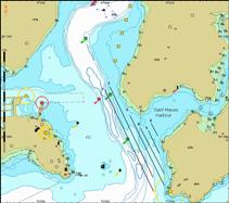
Figure 2.1: Map of survey area showing sidescan sonar transect lines (click to enlarge) |
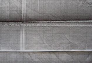
A benthic survey of the Fal estuary was carried out onboard the RV Explorer. Six transect lines, each between 1 and 2 miles long were surveyed in the area from East Narrows to Shag Rock (see figure 2.1). A sidescan sonar with a frequency of 100kHz and a total swath width of 150m and a 75m slant range was used to map the sea floor along the transect lines. The resultant sonograph was used to determine grab sample locations. Due to adverse weather conditions in the estuary only 2 of 4 planned grab samples were executed using a Van-Veen grab (grab 1: 50°08.845N, 05°01.137W; grab 2: 50°08.655W, 05°01.164N). Furthermore, video footage from an underwater camera attached to a CTD rosette was used to confirm benthic habitat boundaries while the boat drifted. The track plot of the video can be seen in figure 2.2. The video data revealed more diverse floral and faunal assemblages than the grab samples. |
|
Tides
|
Weather Conditions
|
|
Aims
|
Equipment
|
|
Crew Sonar Deployment: Joe Green Sonar Analysis: Allison Martin, Arwen Bargery, Emma Steventon Grab Deployment: Emma Steventon, Emily Savage Grab Sample Analyst: Allison Martin, Arwen Bargery, Rosanna von Zweigbergk Video Master: Joe Green and Doug March Position coordinator: Doug March, Andrew Ashdown. Logbook: Marcus Sampson |
|
|
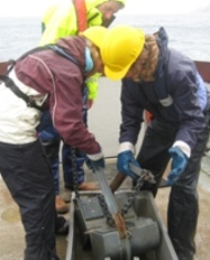
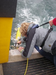
Method A total of 6 transects were made between East Narrows and Shag Rock crossing the outlet of Saint Mawes Harbour (see Route Map). The side-scan sonar was carefully lowered into the water at a depth of 7.5m, 10% of the 75m swath range. The length of the rope was 3.76m and the slant was 45°. The offset was approximately 1.5m. Each transect stretched for approximately 1-2 miles. The printout from the sonograph was continuously monitored and points of interest were recorded as potential grab sampling sites. During each transect the latitude and longitude was recorded every two minutes to allow our position to be recorded. Ground truthing was performed at two grab sites determined by previous interpretation of interesting areas on the sonogram. A Van-veen grab was deployed and the grab sample was analysed on deck, sieved and photographed. The sediment grain size was determined and the main fauna then identified. To compliment the side-scan sonar results, a video camera was lowered and video footage of the sea floor was recorded while the vessel drifted for 6 minutes around grab site 2. Due to bad weather conditions we were unable to deploy the boomer to get a seismic reading. |
|
![]()
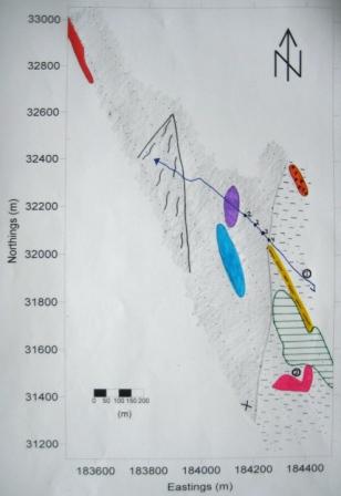
The sonogram resulting from the side scan sonar was used to create a bathymetric track plot (figure 2.2). This plot shows location of the major features seen from the sonogram with corresponding descriptions of each feature.
|
Figure 2.2: Bathymetric Track Plot showing major seafloor sediment types, features and video track plot. |
Figure 2.3: Bathymetric Track Plot Key |
|
Large Scour Marks (Transect 1) A series of 5 large scour marks parallel to one another can be seen in Transect 1. They have a large, gentle depression with a marked sharp incline at the far end, facing a north-east direction. The scours have an average area of 40m by 30m and the total depth of the depression is relatively small, not exceeding more than a meter. The scours are larger than anchor marks and possibly originate from large-scale sediment movement but it is impossible to interpret with this level of surveying. |
Fine sediment and seaweed (Transect 2 and 3) Traversing transects 2 and 3 is a pale area of diameter 174m by 34.5m. There is a gradual fade in tone suggesting this to be the low reflective value of fine sediment. The surrounding darker shading covers an area of approximately 224m by 57m and is thought to be seaweed amid the maerl bed. However, there are other explanations such as smooth rock exposed by hydrodynamic processes or a scour hole. Exact identification could only be achieved through further investigation. |
Lineations (Transects 1, 2 & 3)
Traversing Transects 1, 2 and 3 are large scale linear shallow grooves. The grooves generally trend to the northwest and appear to spread from a single point. They vary in length from 30m to 200m and are spaced approximately 46m apart. The water depth above them is relatively shallow at 1.9m. The grooves depress and then have a short, steep westerly facing slope covering a total area of 0.018km. It is likely that these lineations are transient and could well be caused by helical currents. This results from the flood tide that causes a secondary, transverse helical current asymmetrical to the main Carrick Roads flow. The helical current movement causes scouring of the sediment to occur. |
Bedrock outcroppings, (Transects 5 and 6):
In the Eastern region of the mapping area is a series of high backscatter images of varying size. Lineations observed within these regions can be connected and show a southeast/northwest trend. These areas of high backscatter may represent subdued bedrock outcroppings. The bedrock geology found in and around the Fal estuary is largely structurally controlled and primarily composed of slates. Axial planar cleavage striking to the southwest and dipping at ~50 degrees in the area is dominant over bedding planes, virtually erasing them. The coincident orientations of cleavage planes and areas of high backscatter readings suggest bedrock outcroppings are the most accurate interpretation. In the most North-Eastern region of the mapping area (Transect 6) lunate bedrock outcroppings are seen. The rounded morphology of these outcroppings observed on the sonar is interpreted to be a result of partial covering by sediment due to the hydrodynamics in the area. Widths range from 80 to 105m but the lengths of the features could not be determined as they continued out of the mapping area. Another possible interpretation of these data is that they are a series of benthic macro floral assemblages. |
|
Figure 2.4: Image Grab Sample 1 |
The sediment in the grab samples (fig. 2.4-2.5) was light grey/brown, moderately sorted and lower fine to lower medium grained muddy silt. Maerl and shell fragments (lithics) were the dominant components in both grabs, with a sheet silicate matrix present and low SiO2 content (<10%). Lithic fragments are relatively non–spherical and display a range of rounded to sub-angular grains though shell fragments can display sharp angularity at times. Grab sites 1 and 2 varied little with the exception of a marginal decrease in shell material noted at site 2 indicating that the site was slightly more sorted than site 1. Macro benthic fauna collected from the grab samples were limited to 4 Veneroid bivalves ranging in size between 5 and 20mm. |
|
Figure 2.5: Image Grab Sample 2 |
![]()
 |
 |
 |
|
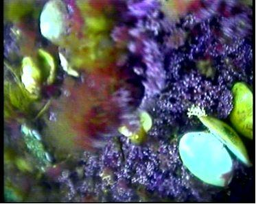
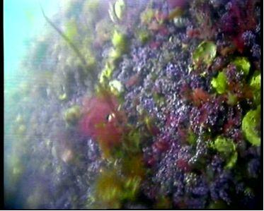
Figure 2.6: There is a covering of Maerl, giving the purple and white background to the area. The colouration of the image is not accurate because the video camera had a light attached that distorted true colour. Thus the Maerl is likely to have been pink in colour, indicating that it was alive. It is also possible to see a species of Rhodophyta (red macro algae) in the background. Scattered in the area are many Macoma clam species (possibly Macoma nasuta). In the foreground, the Macoma clam is open, indicating that it is dead. The clam is a deposit feeder and uses its siphons to draw in sediment from just under the sediment-surface interface. |
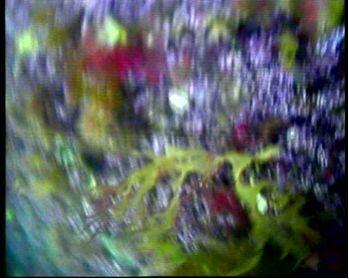
Figure 2.7: There is a single vertical frond of the kelp Thongweed, Himanthalia elongata, in the centre. Centrally surrounding the kelp is more Maerl and Macoma and to the right of the image there is evidence of sponges, possibly of the family Suberites. |
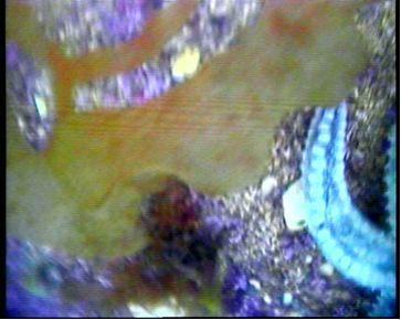
Figure 2.8: In the foreground there is evidence of green macro algae. From what can be seen, this could be Velvet Horn algae (Codium tomentosum). Maerl is also present alongside red macro algae in the background. |
 |
 |
|
Figure 2.9: An arm of a sea star (Asteroidea) is visible in the lower right. It cannot be reliably identified, but we speculate that it is a spiny sea star. |
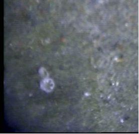
Figure 2.10: the image of the Fanworm species Sabella pavonina is recorded, commonly known as the Peacock Worm. In the live video footage it is possible to see the Fanworm open then close its crown. |
Maerl
|
|
|
The area that was studied displays a clear transitional boundary between dominant substrates which we believe marks the effect of the river input on the physical properties of the benthos. The main feature that was observed was the marked change in sediment type across the linear boundary that runs across all of our transects in a NNE direction. This aligns with the influence of the Percuil River into the main Carrick Roads area. The possible river-influenced sediment, to the west of the boundary, appears to be coarser according to the sonar return. On the east side of the boundary, the area on the sonar is markedly lighter, implying finer sediment. On the east side of the boundary, our two grab samples were collected and confirmed the sediment type as being fine silts and muds. On the west side of the boundary, the video camera was deployed and observed large expanses of maerl beds. Thus the darker area of back scatter has been influenced by the high return from the calcareous maerl as well as a difference in sediment type. There were a number of individual features that were observed and have been discussed as separate entities. What is apparent is that the area undergoes a continuous variable weather pattern and hence changing hydrodynamics in the area. Therefore many features are transient and can change from day to day. It is important to note that the area is very active in terms of on-going anthropogenic influences such as the constant shipping, naval and leisure activities occurring in the Fal estuary which impact the benthic structure considerably. |
![]()
|
|
|
|
Date: 8th July 2008
PSO: Joe Green (RV Bill Conway) and Doug March (Ocean Adventure RIB)
|
Introduction |
|
The physics, chemistry and biology of the water column in and around the Fal estuary were investigated on board the RV Bill Conway, and the Ocean Adventure RIB. The Fal Estuary is fed by a large number of rivers, creeks and tributaries. The Turo and Fal River were included in our study directly, whilst other riverine influences were taken into account by examining their impact on the main estuary. Despite this, the Estuary has little freshwater influence being tidally dominated. Furthermore, many frontal systems were found during the survey and their properties were investigated. |
|
Tides
|
|
Aim
|
Equipment
|
|
|
RIB Crew PSO: Doug March Logbook: Doug March Equipment Deployment: Andy Ashdown, Rosanna Von Zweigbergk Chemists: Andy Ashdown, Rosanna Von Zweigbergk |
Conway Crew PSO: Joe Green Logbook: Arwen Bargery, Joe Green Chemists: Allison Martin, Emma Steventon Computer Master: Alex Bryk, Arwen Bargery Computer Analyst: Alex Bryk Secchi Disk: Allison Martin, Joe Green Equipment Deployment: Emily Savage, Marcus Sampson |
|
|
Map of transects and stations
Click to enlarge |
||
|
Method The team was split in two, with three scientists on the RIB and seven on the Conway. Alongside surveying the Fal estuary, the RIB surveyed the Truro River and the Conway surveyed the mouth of the Fal River, to collect samples of a more freshwater origin. The freshwater input in this area is low, therefore a sample was also collected from the Truro River at an earlier date to establish a riverine end member to calibrate the data. Eleven transects across the estuary and aforementioned rivers were done in total and surface samples were taken at various locations along the transects. Surface samples were also taken at substantial changes in salinity. The CTD and T/S probe were deployed to create a vertical profile of the water column and samples were taken at points of certain interest. Each collected water sample was prepared onboard for processing the following day according to the laboratory methods described above. Data was then analyzed and major trends were investigated. |
||
|
The whole Fal region is heavily enriched in nutrients through anthropogenic influences. The main sources of nutrients to the area are primarily diffuse. The agricultural influence particularly affect the nitrate values. Additionally there is impact from point source local sewage outputs and industrial sources (fig. 3.1). The sewage has most impact on the phosphate levels in the area, whilst the nitrate is more heavily affected by the agricultural sources. The nutrient status of the area is not only affected by the anthropogenic chemical input into the area but also by physical parameters such as the local geology and sediment type, land usage, volume, dilution and flushing rate, rainfall, vertical mixing, and wave exposure (fig. 3.2). These things are almost always individual to the area and highly variable seasonally. This means that not all variations in nutrients can be predicted or explained due to there being so many contributing factors.
Figure 3.2: Estimated sources of estuarine nutrients. (Langston et al, 2006) |
Figure 3.1: Effluence in the Fal Estuary Region: showing some of the larger discharge consents to the Fal estuary. The open symbols represent sewage discharge and the closed symbols represent heavier outputs of trade consents and miscellaneous sources of effluent (Langston et al, 2006).
|
|
![]()
|
Transect 1 |
|
|
Magnitude |
Direction |
|
Magnitude is highest at the sea surface near entrance to the bay (0.25-0.375 m/s). This may be as a result of the input of the River Percuil through St Mawe’s harbour. In addition, the lack of fast moving water at depth may be a result of friction from the seabed. The remainder of the water column is dominated by water travelling below 0.0-0.125 m/s. |
At the east and west end of the ADCP transect taken, there is a switch in direction from 90o due east, to near 180o due south. We suggest that this is as a result of the inputs of the two rivers at either end. In the centre of the channel at the surface the average flow is to the east and coincides with the wind direction at this time. At depth in the channel a northerly flow into the bay can be observed. The Black Rock ADCP transect here was taken during slack water on the turn from flood to ebb tide. This northerly flow may be a result of the lag-time associated with turning tides manifesting itself in a residual inflowing current from the previous flood tide. |
|
Figure 3.3: Transect 1 ADCP Velocity Magnitude (click to enlarge) |
Figure 3.4: Transect 1 ADCP Velocity Direction (click to enlarge) |
|
Backscatter |
|
Backscatter throughout the water column is generally low (56-66dB). However at the point, which is roughly south of the St Mawe input, which is where station 1 is position, slightly higher backscatter is found (70-80dB). The suggestion is that the backscatter is caused by zooplankton feeding on a phytoplankton bloom in the area. It is additionally possible that the backscatter is caused by minor flocculation as the water leaves the St Mawe. |
|
Figure 3.5: Transect 1 ADCP Backscatter (click to enlarge) |
|
Transect 6 |
|
|
Magnitude |
Direction |
|
At this point the water depth was approximately 15m and getting shallower. On the river bed the velocity magnitudes are at their lowest, between 0.0 – 0.125 m/s. In the deeper areas of the river surface velocity is increased (0.2-0.4 m/s) down to about 10m depth. |
We took this transect at 12:24, this meant that the tide was going out, from high tide at 09:09. This means that the dominant flow is at 180o from north and thus out of the estuary. This is consistent throughout the water column. |
|
Figure 3.6: Transect 6 ADCP Velocity Magnitude (click to enlarge) |
Figure 3.7: Transect 6 ADCP Velocity Direction (click to enlarge) |
| Backscatter |
|
Backscatter is through 60-70dB throughout the water column. However at approximately 7.5m depth in the channel a peak in backscatter can be observed. We speculate that this might be because of flocculation from the riverine input. |
|
Figure 3.8: Transect 6 ADCP Backscatter (click to enlarge) |
|
Transect 7 |
|
|
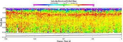
Magnitude |
Direction |
|
The velocity magnitude varies a great deal through the water column on transect 7. Located on a river meander the velocity towards the outside of the bend increases greatly at the surface and down into the water column (~0.5m/s). Towards the inside bend of the velocity decreases slowly to a patch (0.250-0.375 m/s) and then slows almost to a stop (0.0 – 0.125 m/s) at the shallowest point. The tide is in full ebb flow at this point. As expected the speeds towards the outside of the bend were increased by the centrifugal force associated with redirected flow. |
Flow direction is uniform throughout the water column and follows the direction of the ebb flowing tide. |
|
Figure 3.9: Transect 7 ADCP Velocity Magnitude (click to enlarge) |
Figure 3.10: Transect 7 ADCP Velocity Direction (click to enlarge) |
| Backscatter |
|
Backscatter throughout the water column is uniform at approximately 67dB. No major anomalies were recorded We do not observe much fluctuation other than much higher backscatter at the much shallower end. |
|
Figure 3.11: Transect 7 ADCP Backscatter (click to enlarge) |
|
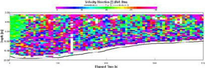
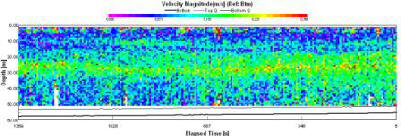
Longitudinal Transect |
|
|
Magnitude |
Direction |
|
The magnitude of velocity increases down the channel along the transect from north to south. A general trend shows higher speeds at the surface (0.250-0.500 m/s), with a net decrease in velocity nearing the river bed. At approximately 200 seconds along the transect a meander bend noticeably increased the flow velocity throughout the water column. This occurs again at roughly 1100 seconds into the transect |
There are three significant features found in this section of the estuary with respect to the direction of flow. As the river encounters meander bends, transverse eddy formation in a circular pattern is recorded. In deep narrow sections of the river, bidirectional flow is recorded. There is a significant but slow travelling bottom flow and a relatively more rapid surface flow. This suggests a saline intrusion along the bed, with slightly fresher water flowing above it. When the channel becomes shallower again a spin in direction can be seen just before the corner, which suggests a possible eddy in the area. |
|
Figure 3.12: Longitudinal Transect ADCP Velocity Magnitude (click to enlarge) |
Figure 3.13: Longitudinal Transect ADCP Velocity Direction (click to enlarge) |
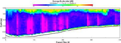
| Backscatter |
|
Backscatter values are low at the end of the transect (60-70dB). In the centre of the transect, values decrease again (62-67dB), then progressively increase. The maximum values are found at the beginning transect (79dB). No distinct formations appear in this region of the estuary. |
|
Figure 3.14: Longitudinal Transect ADCP Backscatter (click to enlarge) |
ADCP Discussion
|
The purpose of recording a longitudinal transect down through the Fal river and into the estuary was to describe the complexities associated with river dominate estuarine circulation in the upper Fal estuary. The dominant features observed here were bi-directional flow in narrow linear regions of the river, and transverse circulation or turbulent eddy formation on meander bends. As the estuary approaches low water a subdued northerly bottom flow is noted in multiple linear regions of the river showing the incipient flood tide. This bottom flow is disrupted on meander bends due to eddy formation enhanced by stream inputs on either side. Other notable observations include possible fluctuation layers lying just above the halocline located at the mouths of small streams entering the northern reaches of the Fal estuary. |
![]()
 |
|
Fronts were observed in several locations up the Fal river and into the Truro river. The most defined of which were discovered as the Truro became the Fal. Fronts occur where there is a large horizontal change in one of the following properties of the water; salinity, temperature, turbidity, flow strength or direction. It was hard to identify which of these properties were causing the fronts we observed. This was because of the dynamic nature of the front and the fact it did not penetrate deep enough to be displayed on our ADCP transect. |
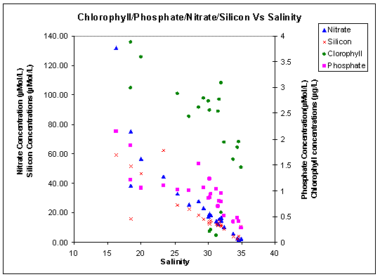
Nutrient Mixing Diagrams
Thee estuarine nutrient data was processed in relation to surface salinity. Due to equipment malfunction of the CTD, only surface nutrient data was considered as being valid for use. Mixing diagrams have been created to display the mixing nature of each of the limiting nutrients (phosphate, nutrients and silicate).
|
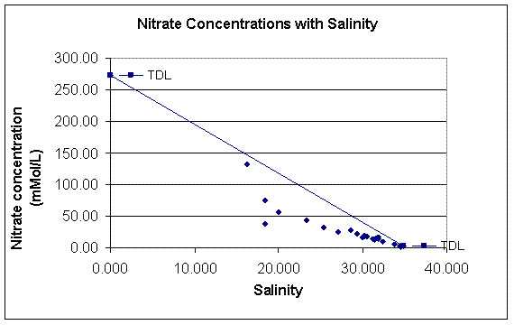
Figure 3.15: Nitrate Mixing Diagram (click to enlarge) |
Nitrate The nitrate mixing diagram (figure 3.15) also shows non conservative behaviour in the Fal estuary (fig. 1.3). The nitrate concentrations all fall below the TDL, showing that there are uptake processes occurring in the estuary, possibly by phytoplankton. This must mean that the effect of nitrate addition is not as dominating a feature in the area as the effect of the phosphate addition. It must be remembered that the riverine end member concentration may have been particularly high due to the high levels of precipitation that had been occurring in the days prior to and subsequent to our sampling . This means that the TDL may be particularly high, because the wash down of increased nutrients from the effect of the precipitation will take several days to fully affect the nutrient concentrations further down stream. The highest nitrate concentration is at site 21 (2.15µMol/L), just below Truro, similarly to the phosphate pattern. The nitrate follows a conservative mixing pattern from site 12, from a salinity of 18 upwards, out to sea. |
|
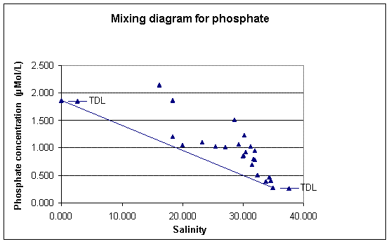
Figure 3.16: Phosphate Mixing Diagram (click to enlarge) |
Phosphate The phosphate mixing diagram (figure 3.16) displays a non-conservative mixing pattern in the Fal estuarine environment (fig. 1.4). The theoretical dilution line (TDL), runs from the riverine end-member, taken from Truro River, at a salinity of 0, to the seaward end member, found at station 1 with a salinity of 34.9. The phosphate concentrations, taken up the River Fal and into the Truro River, do not follow the TDL but rest markedly above it. This suggests that addition is occurring in the estuary. The concentration at station 21, up the Truro river, was by far the highest (131.76µMol/L) and the data follow a fairly conservative pattern from this input source out to sea. There is a large sewage outfall at Truro (upstream of site 21), this can be seen on figure 1 (Effluent in the Fal region). This explains the high levels of phosphate coinciding with this large input. There are also several smaller sewage outfalls further down the Fal River. |
|
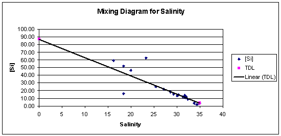
Figure 3.17: Silicon Mixing Diagram (click to enlarge) |
Silicon The silicon mixing diagram (figure 3.17) shows that there appears to be silicon addition somewhere up river, possibly due to diatom re-dissolution after a spring bloom. From salinity 15-35, the Silicon behaves roughly conservatively, possibly with some removal possibly caused by diatoms. At salinities 18.4 and 23.3 there are two anomalous data points. The sample at 18.4 was taken from near the entrance of the river Fal so the sample could have been mostly Fal water which potentially could have contained a lower concentration of silicon than the Truro. |
|
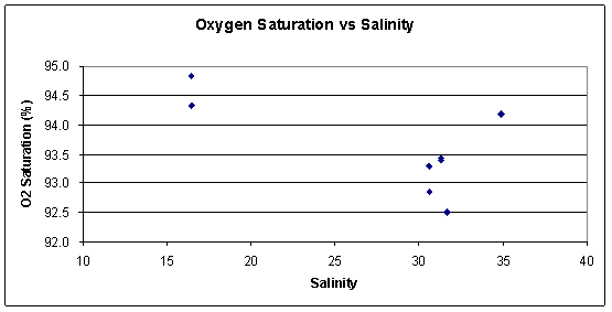
Figure 3.171: Oxygen Saturation vs. Salinity (click to enlarge) |
Oxygen The highest oxygen concentrations correspond with our nutrient and chlorophyll measurements. As seen on figure 3.171, the largest concentration of oxygen is at site 21, where there were also the highest concentrations of chlorophyll and nutrients. This is explainable as the bloom in phytoplankton, results in an area of high primary productivity, which means that there is a high production of oxygen. Only a few oxygen samples were taken and thus definite patterns are hard to depict. Oxygen is also heavily variable depending on many factors. Firstly the timing of the bloom affects it, if the bloom has started to die off and bacterial decomposition has started, then oxygen is utilised and falls. Also the river flow and level of mixing affects the amount of oxygen addition to water, as water column turnover causes subsequent oxygen incorporation from the over lying air. |
Nutrient Discussion
|
Figure 3.18 Mixing Diagram (click to enlarge) |
|
Overall, nutrient mixing (figure 3.18) in the estuary followed a non-conservative mixing pattern. As a result of sewage discharge, the phosphate mixing diagram displayed non-conservative addition. In contrast, nitrate distribution in the estuary exhibits areas of removal, presumably from uptake by phytoplankton. In general, it can be concluded that the nutrient mixing pattern in the Fal estuary is affected by anthropogenic input and the impact of sewage discharge is evident. Diatoms dominated the estuarine area of Falmouth and Truro River, having a visible effect on silicon concentrations by causing removal of Silicon at locations of peak diatom densities. The diversity of phytoplankton groups was lower in the estuary than offshore. The ADCP highlighted some interesting hydrodynamic aspects in the estuary. Interesting backscatter patterns were recorded where the Cowlands and Lamouth Creek enter the estuary, maybe indicating freshwater flocculation. A centrifugal force increasing flow velocity was also encountered at the same location. Between Channals and Tolcarne Creek the backscatter was indicative of gyre formation. Dual layer formation appeared to be occurring in deeper waters near the oyster farms. |
![]()
Phytoplankton
|
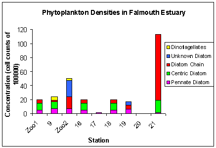
Figure 3.19: Phytoplankton speciation results |
Phytoplankton Discussion
|
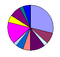
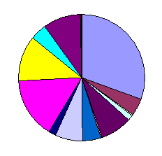
The samples taken from the Bill Conway are stations Zoo1, 9 and Zoo2. All the remaining stations are taken from the rib. The general trend shown in figure 3.19 that diatoms dominate over dinoflagellates at all stations sampled, which is similar to that found in the offshore study. Dinoflagellates are present at only two of the nine stations sampled (stations 5 and Zoo2) and ciliates, which were present in low concentrations in the offshore study, are completely absent from the estuarine samples. The most abundant phytoplankton group is found at station 21 and is the diatom chains which consist of species such as Thallassiosira sp. A potential cause for the high densities at this site is the close proximity to the Truro sewage outfall resulting in exaggerated nutrient concentrations in this area (Langston et al., 2006). Despite this, they are not evenly distributed across the sampling sites, as site 21 had 9,400,000 cells compared to just 200,000 at station 9. This correlates well to the data in the silicon mixing diagram which indicates high levels of silica removal at salinities of 18. The extreme high levels of diatom chains at station 21 compared with other stations is a potential reason for the silica removal in this area. The mixing diagram also indicates addition of silica in the region of mid salinities. A possible explanation for this is that diatoms that originated in the lower salinity waters were unable to tolerate the increasing salinities when they were carried downstream and so the silicious content of their frustules dissolved into the water column, therefore increasing the silica content. The pennate and the centric diatoms, unlike the diatom chains are fairly evenly distributed across all the stations, with the pennates averaging from 500,000-700,000 and the centric diatoms, when present are usually at 100000 cells. The station with the lowest phytoplankton abundance is station 20 which indicates that no phytoplankton species were present. These lowest phytoplankton densities support lowest zooplankton densities. Chlorophyll, Silicate, nitrate and phosphate concentrations are all highest at station 21. This is the lowest salinity station and is also the site at which centric and chain diatom densities are highest. Nitrate shows levels of removal at salinities between 16 and 35. It is difficult to conclude whether depletion is phytoplankton related as the range of salinities sampled was restricted (Head, 1985). All the samples fall within the salinities where depletion is occurring so it can only be concluded that the phytoplankton present contribute to removal. Phosphate on the other hand shows significant addition to the water column, so any removal by phytoplankton is counteracted by external sources to the water column, which are further explained in the nutrients section. |
![]()
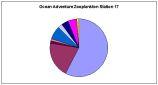
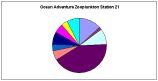
Zooplankton
|
Figure 3.20: Zoo 1 Phytoplankton Chart (click to enlarge) |
Figure 3.21: Zoo 1 Phytoplankton Chart (click to enlarge) |
Figure 3.22: Zoo 17 Phytoplankton Chart (click to enlarge) |
Figure 3.23: Zoo 21 Phytoplankton Chart (click to enlarge) |
Zooplankton Discussion
|
There is a progressive reduction in zooplankton density with decreasing salinity for the Bill Conway but an increase in density with decreasing salinity from the rib samples. Disregarding the first rib sample (figure 3.22) which is of similar salinity to the first Conway sample, there is a progressive decline in density with declining salinity. The greatest density of zooplankton was found in the most seaward sample at site Zoo1 (figure 3.20), where densities were six times those of site Zoo2 (figure 3.21) , a site further up the estuary, in lower salinity waters. At sites Zoo1, Zoo2 and 21 (figures 3.20, 3.21 and 3.23), the most dominant group is the Copepoda, compared to Cirripedia larvae at site 17 (figure 3.22). The cirripedia are the second most dominant group at sites Zoo1 and Zoo2 but are in low concentrations at Site 21. They are also in much higher densities at site Zoo1 than they are in any of the offshore samples. Decapoda larvae are highly prevalent (363 organisms) at site Zoo, but absent from sites Zoo2 and 21with only 8 present at site 17. The zooplankton densities in the offshore waters exceed those of the estuarine waters in all samples apart from offshore station 4 between 28-0m. The densities at this offshore station are exceeded by site Zoo1from the estuarine samples, although the diversity is still greater in the offshore sample. The likely explanation for this is that the estuarine samples were all taken from the surface, where irradiance levels are high, whereas the offshore samples were taken from various depths. Through calculation of a Simpsons Diversity Index, it has been found that diversity is greatest at site Zoo, with an index of 0.85. This is equal to the highest diversity index found at any of the offshore stations. However, despite the high diversity index, there are a number of species found within the offshore samples that were absent from any of the estuarine samples. Examples of these include, Cladocera, Echinoderm, Appendicularia and Fish larvae and Ectoprocta. The diversity was lowest at site Zoo2, in which only 3 species were identified. The diversity followed the same pattern as salinity in that it decreased with decreasing salinity in the Conway samples and the rib samples independently. At station Zoo1, where zooplankton numbers are greatest, corresponding phytoplankton numbers are low. This could be attributed to rapid zooplankton grazing on phytoplankton, hence the two extremes of populations. However, it is likely that if this station was re-sampled soon, the zooplankton population would be declining due to the low phytoplankton population being unable to support such vast zooplankton numbers. The high nutrient values at site 21 could be the result of sewage outfall from Truro, which could lead to eutrophication in the area (Langston et al., 2006). These high nutrient values are supporting a potential bloom of phytoplankton which will eventually deplete as they are grazed down by zooplankton. This is a possible explanation for the low zooplankton densities at site 2, as the population dynamics have not yet benefited from the dramatically increased grazing supply available to them. |
![]()
Final Conclusion
|
We hope that our findings may be of use to any potential developers or conservationists in the Fal estuary who are interested in the biological, chemical and physical aspects of Falmouth waters. |
|
Aelbrecht, D., D'hieves. G.C., Renouard, D., 1997. 'Experimental Study of the Ekman layer instability in steady or oscillating flows', Contential Shelf Research, 19, p. 1851-1867. Baschek, B., Farmer, D.M., Garrett, C. Tidal fronts and their role in air-sea gas exchange. Journal of Marine Research. 64, p. 483-515. Colebrook, J.M., 1979. 'Continuous Plankton Records: Seasonal cycles of phytoplankton and copepods in the North Atlantic ocean and the North Sea', Marine Biology, 51, 1, p. 23-32. Gibbs, P.E., Bryan, G.W., Pascoe, P.L. and Burt, G.R. 1987. The use of the dog -whelk, Nucella lapillus, as an indicator of tributyltin (TBT) contamination. Journal of the Marine Biological Association of the United Kingdom. 67 (3), p.507-523. Grasshoff, K., Kremling, K. and Ehrhardt,M., 1999. Methods of Seawater Analysis. 3rd ed. Wiley-VCH, pp. 632 Haward, P., Nelson-Smith, T. and Shields, C., 1996. Sea Shores of Britain and Europe. Head, P. C. 1985. Practical Estuarine Chemistry: A Handbook. Cambridge University Press. Jackson, A. 2007. Phymatolithon calcereum. Maerl. Marine Life Information Network: Biology and Sensitivity Key Information Sub-programme [on-line]. Plymouth: Marine Biological Association of the United Kingdom. Last accessed 10/07/2008. Available at www.marlin.ac.uk/species/Phymatolithoncalcareum.htm. Johnson K. and Petty R.L., 1983. Determination of nitrate and nitrite in seawater by flow injection analysis. Limnology and Oceanography, 28, p. 1260-1266 Langston, W.J., Chesman, B.S., Burt, G.R., Taylor, M., Covey, R., Cunningham, N., Jonas, P. and Hawkins, S.J. 2006. Characterisation of European Marine Sites: The Fal and Helford, (candidate) Special Area of Conservation. Marine Biological Association of the United Kingdom. Parsons T. R., Maita Y. and Lalli C., 1984. A manual of chemical and biological methods for seawater analysis, Pergamon, pp. 173 Sharples, J. and Simpson, J.H. 2001. Shelf-Sea and Slope Fronts. Encyclopedia of Ocean Science, p. 2759-2768. [online]. Available at www.sciencedirect.com. Last accessed: 10/7/08. |
![]()
|
he views and opinions expressed on this website are those of the authors' own and do not necessarily represent the views and opinions of the University of Southampton, it's staff or any of it's affiliates. |

 The Fal
estuary is the country's deepest estuary and also the third largest natural harbour in the world.
Six major tributaries converge at the Fal Estuary, which flow into the lower reaches known as Carrick Roads, the deep
channel that extends from depths of 12m at Turnaware
point to 34m at the
southern end. The estuary experiences a macrotidal tide regime in the lower regions up to the
Falmouth area, with a maximum springs tidal range of 5.3m and a mesotidal
regime at Truro, with a spring tidal range of 3.5m.The mean sea surface
temperature for the area in the summer is 16ºC. The temperature is largely
unvaried due to the low freshwater input.
The Fal
estuary is the country's deepest estuary and also the third largest natural harbour in the world.
Six major tributaries converge at the Fal Estuary, which flow into the lower reaches known as Carrick Roads, the deep
channel that extends from depths of 12m at Turnaware
point to 34m at the
southern end. The estuary experiences a macrotidal tide regime in the lower regions up to the
Falmouth area, with a maximum springs tidal range of 5.3m and a mesotidal
regime at Truro, with a spring tidal range of 3.5m.The mean sea surface
temperature for the area in the summer is 16ºC. The temperature is largely
unvaried due to the low freshwater input. 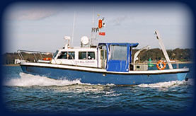

.jpg)
.jpg)
.jpg)