|
CTD Analysis
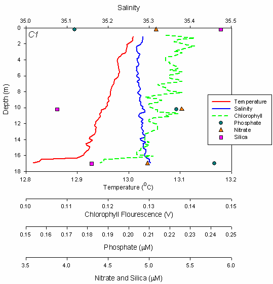
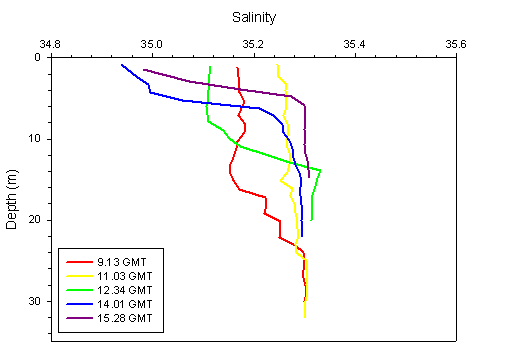
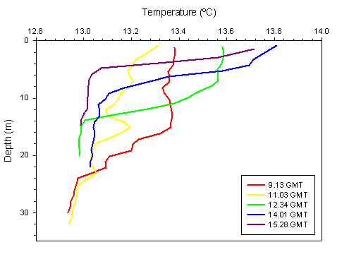
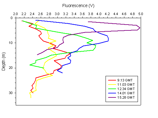
The profile of salinity, temperature and
fluorescence in the water column is plotted against depth (Fig. 13,
14 and 15), with separate profiles showing the progression of the
halocline as the tidal cycle continues. We begin with the red line,
which is the profile as determined by a CTD cast at 09.13GMT (before
HT). The yellow, green, blue and purple plots show the profile at the
same point at 11.03, 12.34, 14.01 and 15.28GMT respectively. High tide
is at 11.56GMT so the majority of the tidal cycle is covered.
The 09.13GMT (red) profile demonstrates
a slight stratification in the stable water column with slightly lower
density, with slightly warmer water in the surface layer. A chlorophyll
maximum is observable at 14m, around the level of the thermocline. This
is in agreement with the Euphotic depth estimated from the Secchi disk
data (estimate of 14.8m).
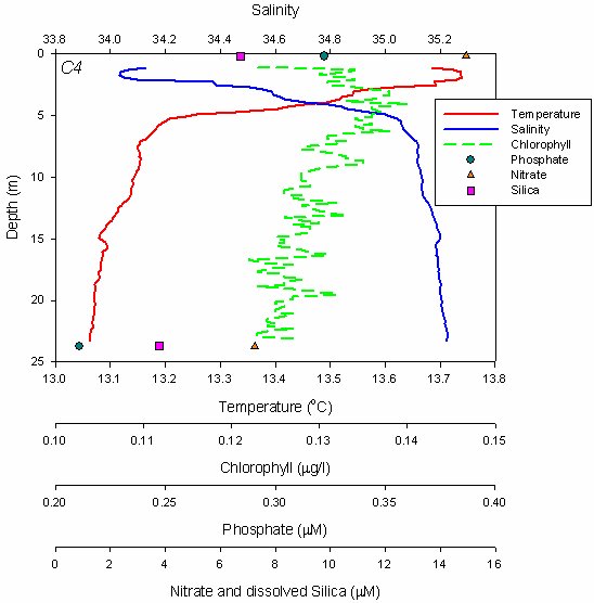
The 11.03 GMT (yellow) profile was taken
shortly before high tide and the discharge from riverine input is
minimal at this time. The homogeneity of the vertical profile and the
high salinity are indicative of an influx of marine water. The reduction
in temperature compared to the last profile is due to the colder
seawater entering into the mouth of the estuary. The chlorophyll profile
is similar to that of the red line, although the plankton are better
distributed throughout the water column rather than having a very
obvious maximum at one particular depth.
The green profile (12.34 GMT) was
obtained after high tide, so the tide is ebbing at this time. The
salinity in the surface ten metres decreases slightly compared to the
last profile, perhaps due to the riverine water which should be
beginning to penetrate the lower reaches of the estuary, although the
mixing of fresh and saline water along the gradient of the estuary
reduces the signal of the freshwater ‘spike’ to a fraction of a salinity
unit. A corresponding increase in temperature supports this observation
as freshwater is generally expected to be warmer than seawater. A
notable chlorophyll maximum is present at the base of the Euphotic zone
(~11-12m) again corresponding to the observation made with Secchi disk,
in this case 13.5m.
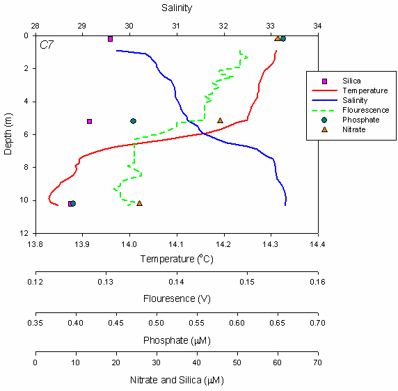
The blue profile (sampled at 14.01 GMT)
shows a continuation of the out flux of freshwater in the surface. An
increase in the rate of out-flowing water compared to the last is to be
expected because the tidal cycle is moving towards low tide. Again, this
freshwater signal is accompanied by a significant increase in
temperature. Due to the combined salinity and temperature difference,
the water column is very stable in our sample zone at this time. The
phytoplankton find themselves at the thermo/halocline with a chlorophyll
maximum at the same depth (8-10m), which is supported by the Secchi
Euphotic depth (10.5m).
The last profile (in purple) that we
obtained was at 15.28 GMT. Once again, a spike of warm, freshwater is
highly visible in the surface layer, where there is also a high
concentration of chlorophyll. The high nutrient concentration in the
freshwater permits a large bloom of plankton in the surface layer, at
around 4 metres. However, the Euphotic depth predicted from the Secchi
disk was this time at about 12m depth. An operational error could be to
blame for this difference.
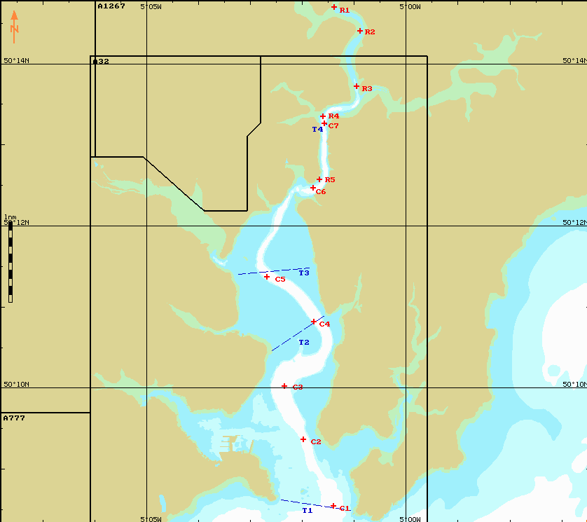
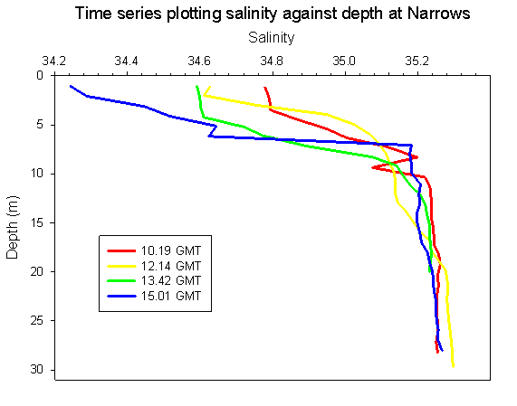
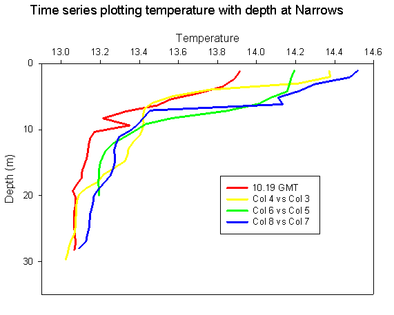
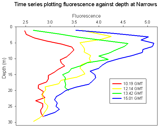
In addition to the points
collected at Black Rock, a regular CTD cast was performed at the Narrows
(roughly 50° 09.450N, 005° 02.100W) with 4 profiles. The first cast
(red) was performed at 10.19 GMT. The second cast (yellow) was performed
at 12.14 GMT, after HT at 11:58 GMT. The third and fourth (green and
blue) casts were performed at 13.42 GMT and 15.01 GMT. Fig. 16
shows the Salinity Time-Series, Fig. 17 shows the Temperature
time-series, and Fig. 18 shows the Fluorescence time-series.
These profiles show similar
patterns to those collected at Black Rock. After the high tide, the
freshwater layer in the surface becomes more prominent and the minimum
salinity decreases. As we were closer to the freshwater end member for
this point, the overall salinity is lower in the surface layer than that
which was observed at Black Rock. Once again, the freshwater layer
flowing over the denser saline layer is warmer than the seawater. There
is a chlorophyll maximum on the thermo/halocline in each profile, which
is generally at about 5-8m depth. However, the depths of the Euphotic
zone obtained from estimations from the Secchi disk overestimated the
chlorophyll maximum.
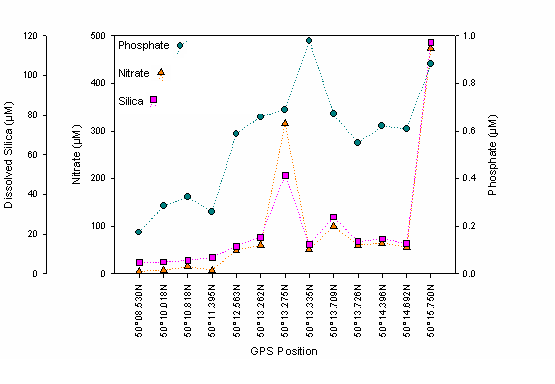
Nutrient concentrations across the time
series at Black Rock
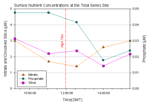 Plotting
surface level nutrient data against the time of sampling demonstrates no
particular relation with the fresh water signal, which had been the case
with the estuarine data set. However this graph allows us to see that
the nutrient concentrations are extremely low even compared to the data
set obtained from the ’Estuarine’ practical. This suggests increased
uptake of nutrients by phytoplankton. Comparing the two Fluorometer
readings would suggest that this is the case. Bearing in mind that the
two Fluorometers are different, they cannot be directly compared.
However the average chlorophyll concentration of all readings taken on
this practical was 6.14µg/L, compared to 4.3µg/L for the ‘Estuarine’
practical, which could explain the apparent increase in nutrient uptake
by photoautotrophs. The much improved weather seems to have allowed the
phytoplankton community to bloom and it is now limited by availability
of nutrients, especially phosphate. Plotting
surface level nutrient data against the time of sampling demonstrates no
particular relation with the fresh water signal, which had been the case
with the estuarine data set. However this graph allows us to see that
the nutrient concentrations are extremely low even compared to the data
set obtained from the ’Estuarine’ practical. This suggests increased
uptake of nutrients by phytoplankton. Comparing the two Fluorometer
readings would suggest that this is the case. Bearing in mind that the
two Fluorometers are different, they cannot be directly compared.
However the average chlorophyll concentration of all readings taken on
this practical was 6.14µg/L, compared to 4.3µg/L for the ‘Estuarine’
practical, which could explain the apparent increase in nutrient uptake
by photoautotrophs. The much improved weather seems to have allowed the
phytoplankton community to bloom and it is now limited by availability
of nutrients, especially phosphate.
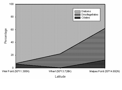
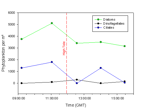
Phytoplankton Levels
Dinoflagellates
numbers show very little variation with time. Looking at the raw data
their numbers seem to increase with depth. This may be due to the
presence of higher nutrients and lower predation and so they may migrate
to the surface at night. Diatoms and ciliate numbers appear to peak
shortly before high tide. This may be due to an influx with incoming
coastal waters on the tide. Numbers drop once more after high tide,
strengthening the suggestion that they are carried on the tide.
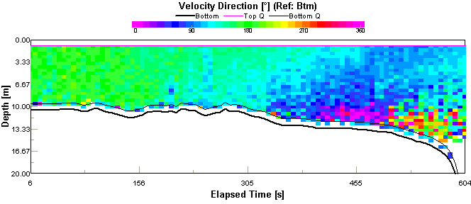
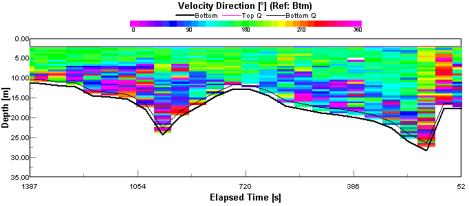
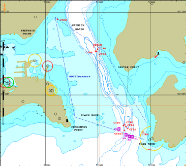
ADCP Transects
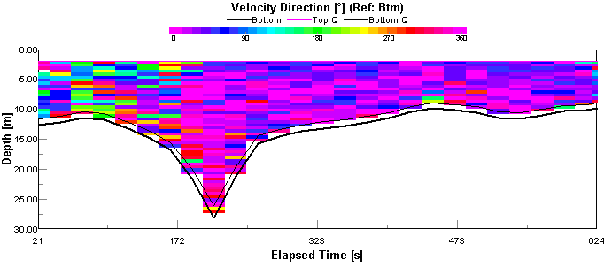
Fig.20. Velocity
direction contour plot – This shows that the net flow of water is
generally northeast, fitting with the tide flooding into the estuary due
to high tide at 11.56GMT. However, nearer to the right shore there is no
general direction, indicating that an eddy may be present.
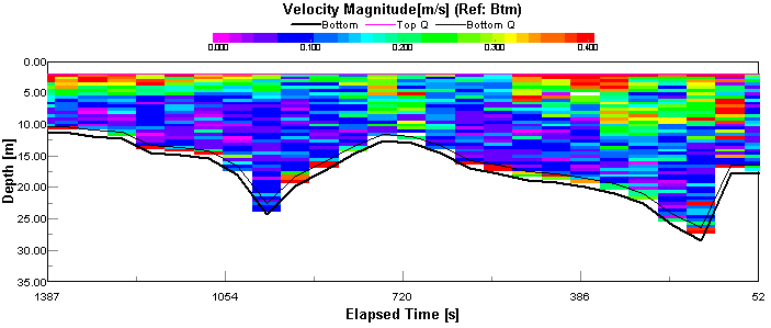
Fig. 21.
Velocity magnitude contour plot – This shows the velocity magnitude of
the flow at transect 1. On the western side the flow is slightly
slower, by ~0.25m/s. Closer to the eastern shore the magnitude increases
slightly, splitting the estuary into faster moving north flowing water
on the left, with a slow moving eddy to the right.
Fig.22. Velocity
direction contour plot – This shows that the main body of water towards
the West is flowing in an easterly direction. On the eastern side of
the estuary the flow is in a north-east direction. On the far eastern
side, the flow is southwards. The tidal forces are at a minimum as we
are just before high tide so there is no particular general direction or
‘main flow’.
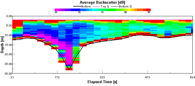
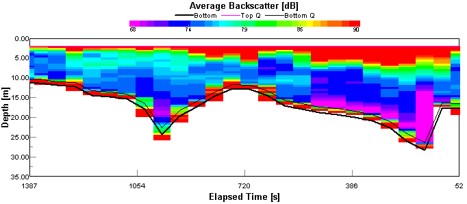
Fig. 23. Average
Backscatter contour plot – An ADCP works by sending out acoustic signals
that reflect back to the transmitting receiver at different frequencies
thus recording a time delay that is converted into velocity.
Backscatter shows the amount of “activity” in the water column that can
affect the quality of the data. At the surface, there is a high amount
of backscatter which is due to surface turbulence, from wind induced
waves. There is a region of low backscatter in the channel, with fairly
low backscatter in the main body of water. In the top ~8 metres of the
water column on the western side of the transect there is a high amount
of backscatter which could be the location of a phytoplankton bloom.
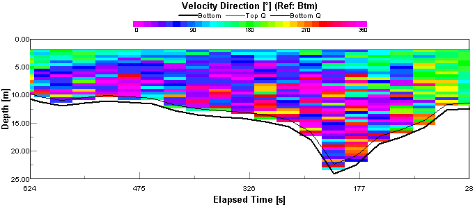
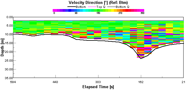
Fig.24.
Velocity direction contour plot – This shows that the net flow of water
is generally south, fitting with the falling tide that occurred at
11.56GMT. The layer of fresh water in the surface is clearly visible
as being a separate water body, as shown in the CTD profiles. However,
nearer to the left shore there is no general direction, indicating that
an eddy may be present, although this could be due to the curve taken at
the beginning of the transect.
Fig. 25. Velocity magnitude contour plot – This shows the velocity
magnitude of the flow at transect 10. The current velocity in the
surface, in the fresh water layer, is much higher than the sea water
intrusion. This stratification is also shown on the CTD profiles.
Although some currents are shown to be present in the denser bottom
layer, they are much smaller in magnitude than the surface layer.
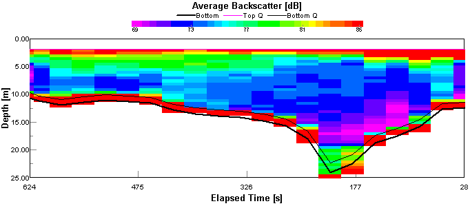
Fig. 26.
Average
Backscatter contour plot – This is a measure of the amount of ‘activity’
within the water column. At the surface, there is a high amount of
backscatter that is due to surface turbulence, from wind-induced waves,
due to fairly heavy south westerly winds. However, the backscatter
towards the left shore of the estuary is significantly higher, and could
be attributed to the high level of chlorophyll present in this fresh
water layer, as shown in the CTD profile.
Fig.27. Velocity
direction contour plot – This shows that the net flow of water is
generally to the south, in this shallower channel of the estuary. The
freshwater out flux is at its maximum as we are approaching the midway
point between high tide and low tide where the rate of tidally induced
flows is at its maximum. The bottom layer is quite turbulent however,
possibly with some kind of eddy.
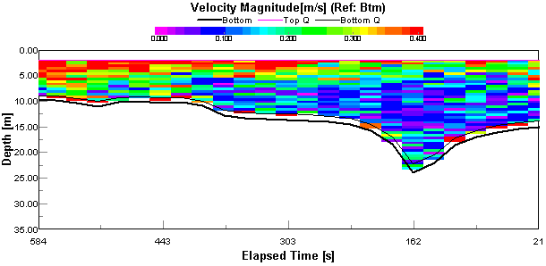
Fig. 28.
Velocity magnitude
contour plot – This shows the velocity magnitude of the flow at transect
14. Again the higher current velocity in the fresher surface layer is
clearly visible as this layer flows out over the bottom sea water layer
due to its lower density.
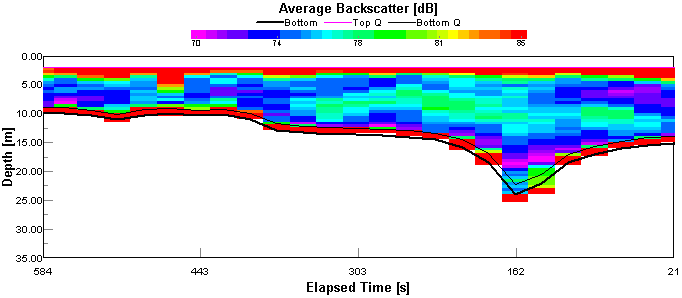
Fig. 29. Average
Backscatter contour plot – At the surface, there is again a high amount
of backscatter that is due to surface turbulence, from wind-induced
waves, due to fairly heavy southwesterly winds. There is a layer of
reasonably isolated backscatter in the middle of the water column, which
is probably caused by phytoplankton. This corresponds to the chlorophyll
maximum at 8-10m as shown on the CTD profiles from Black Rock.
Richardson
Number
The
Richardson Number is a scale that describes the physical conditions in
terms of mixing and stability. If the number is less than 0.25, then
the system is well mixed. If the number is more than 1, then the system
is statically stable. A plot of the Richardson Number against depth can
be compared to the CTD profiles of the corresponding locations to
understand the physical behaviour of the water column. This has been
done for the time series of the transect from Pendennis Point to Shag
Rock.
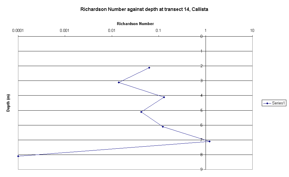
Transect 14 –
profile 10 – 1401 GMT (125 minutes after high water at Falmouth)
There is a
well mixed layer from the surface to ~4m, shown by 3 Richardson Numbers
that are all less than 0.25. There is a sharp increase in the
Richardson number from 0.042 at 5.1m, to 1.21 at 7.1m. This shows
stability in the water column that can also be seen in the CTD profiles,
as a halocline from 35.0 at ~4m, to 35.3 at ~7m. The change in salinity
overall is still very low. A thermocline is also present, from 13.7oC
at ~4m, to 13.0oC at ~9m. However, if the whole of the water
column is well mixed, this stability may be temporary, and may also show
two well mixed bodies of water that are stable in comparison to each
other. This cannot be determined for sure without more practical data.
These two bodies of water allow nutrients to pass from the deep to the
upper water column at ~8.44m, which is coherent with the chlorophyll
maximum as shown on the Fluorescence profile. This is where the
Richardson Number decreases to 0.0001 just below the chlorophyll maximum
depth.
|


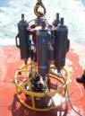 CTD rosette:
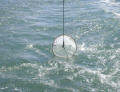
 A
Secchi disk is a low-tech instrument which allows observers to measure
light penetration through the water column without the need for
computers, calculators or even batteries! Essentially, a disk painted
with alternating white and black segments is lowered down by hand over
the side of the vessel. When it disappears completely from sight it is
raised slowly back up until it can be seen again. Distance marks on the
line from which the disk is suspended allow a depth to be recorded. Multiple measurements by several
operators can provide an average, as eyesight varies from individual to
individual. A note is also taken of light levels
which can be affected by changes in cloud cover as this will again
affect the readings. The Secchi depth is generally accepted to be around
one third of the Euphotic zone or "1% depth" below which photosynthesis
cannot take place.
A
Secchi disk is a low-tech instrument which allows observers to measure
light penetration through the water column without the need for
computers, calculators or even batteries! Essentially, a disk painted
with alternating white and black segments is lowered down by hand over
the side of the vessel. When it disappears completely from sight it is
raised slowly back up until it can be seen again. Distance marks on the
line from which the disk is suspended allow a depth to be recorded. Multiple measurements by several
operators can provide an average, as eyesight varies from individual to
individual. A note is also taken of light levels
which can be affected by changes in cloud cover as this will again
affect the readings. The Secchi depth is generally accepted to be around
one third of the Euphotic zone or "1% depth" below which photosynthesis
cannot take place.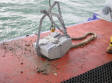
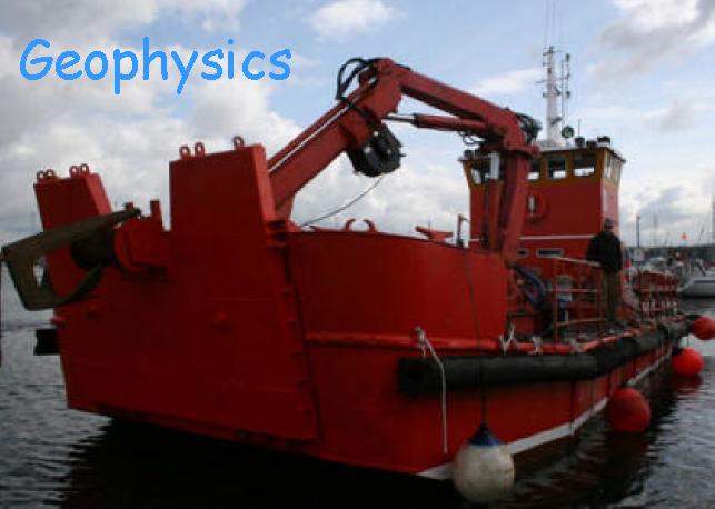
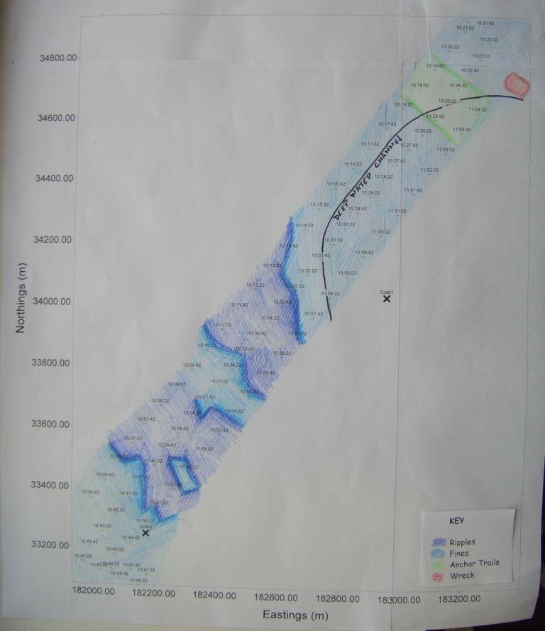
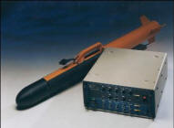 A “torpedo-like” fish is towed behind
the boat, sending out acoustic pulses and receiving the reflections off
the sea bed. The sound pulses are usually on a frequency between 100 and
500 KHz. For the geophysics practical, the frequency used was 500 KHz as
this gave better resolution at the towing depth we used. As the fish is
towed, an image is displayed, showing areas of high returns and areas of
shadow (which represent ripples, bed forms and other objects/bathymetric
features on the sea floor) on a monitor and printed out on paper plot,
which are saved for later analysis. The fish itself can be towed behind
most sized vessels, including RIBs. However, the attendant computer
equipment necessitates a larger vessel with mains power supplies, such
as RV Bill Conway or larger. During this course, MV Grey Bear was used
for this duty.
A “torpedo-like” fish is towed behind
the boat, sending out acoustic pulses and receiving the reflections off
the sea bed. The sound pulses are usually on a frequency between 100 and
500 KHz. For the geophysics practical, the frequency used was 500 KHz as
this gave better resolution at the towing depth we used. As the fish is
towed, an image is displayed, showing areas of high returns and areas of
shadow (which represent ripples, bed forms and other objects/bathymetric
features on the sea floor) on a monitor and printed out on paper plot,
which are saved for later analysis. The fish itself can be towed behind
most sized vessels, including RIBs. However, the attendant computer
equipment necessitates a larger vessel with mains power supplies, such
as RV Bill Conway or larger. During this course, MV Grey Bear was used
for this duty.