Falmouth Field Course 2007Group 8 |
||
|
Rachel Bartram, Tim Beckett, Sam Bevan, David Chanter, Rachel Evans, Matthew King, Joe Kingswood, Conor McCaughan, Sarah Moore, Daniel Stalker |
||


     |
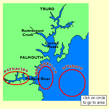
Contents
|
 |
 |
|
|
N.B. All times stated are in GMT and all locations are in WGS84 |
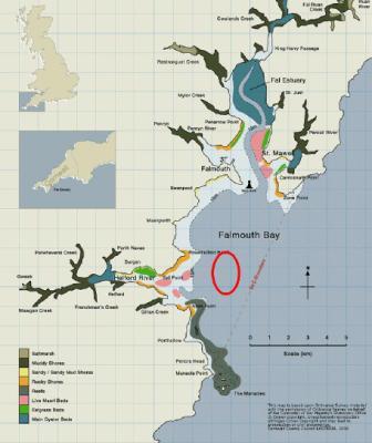
IntroductionThe Helford Estuary is a Ria system located on the South Coast of Cornwall at the Western end of the English channel. This area is a useful scientific study area with several indigenous and alien species that have been placed within a Special Area of Conservation (SAC) including the rare calcareous seaweed, Maerl, rarely found outside of Scotland. The impact of pollution within the area on the pelagic and benthic wildlife has long been studied as a means of monitoring pollution within the region and its effects on the ecology and biota within the system. In the region itself the prevailing winds are South-Westerly due to the nature of the weather systems reaching Britain from the North Atlantic and surface water temperatures in the summer are generally in the region of 16°C with the surrounding offshore waters having a mean salinity of roughly 35. Stratification in the offshore waters is normal in the summer due to the creation of a seasonal thermocline, and this stratification is broken down in the winter due to lower solar radiation inputs and greater turbulent mixing through wind. This seasonal system has a significant effect on the chemistry and biology of the coastal waters. |
| Grey bear - Geophysics - 5/7/2007 | |||||||||||
| Boat Used:
Grey Bear Weather:
Tides:
|
Location:
|
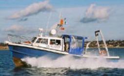
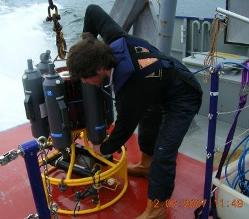
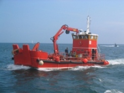 Grey Bear
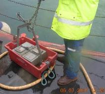
Pictures of the Van-Veen grab on Grey Bear
|
|||||||||
IntroductionThe overall aim was to survey the area just off the Helford River in order to characterise and classify the geophysical features, possibly for use by Natural England. The survey consisted of 5 transects of 2km each. These were spaced 100m apart with a swath width of 150m, producing an overlap of 50m. Onboard a geo-acoustics side scan transceiver box coupled to a Codasys recording system was used to determine the characteristics of the seabed. Our co-ordinates were recorded manually every minute to create a back up of locations in case of a computer failure. A spotter at the back of the boat recorded the time and location of any objects, such as buoys and boat traffic that may have had an effect on the backscatter produced by the side scan. |
|||||||||||
Equipment UsedSide Scan Sonar The side scan sonar is used to locate seabed features and topography. Using output from a transducer, ultrasonic waves produced on one or both sides create a swath across the seabed. Returning signals received are then output on paper or digital readouts creating an image of seabed forms and features. Energy is reflected off the sea bed, thus giving an indication of its nature depending on the proportion of energy that is returned. For a hard substrate such as gravel or sand, more energy is reflected back, this also occurs if the bed is irregular. These areas of high reflection will be darker on the paper traces, whereas if the seafloor is soft mud or clay, for example, less energy will be reflected back, giving lighter areas on the scan map. If the angle of incidence equals the angle of reflection, the sea bed is very smooth, yet this rarely happens. The transducer can be boat mounted, but mounting within a tow fish causes reduction in movement, this could be caused by boat movement such as boat roll. However, we towed the fish, which also allows greater flexibility for deployment within the water column, and specific positioning at depths can give better readings avoiding surface objects such as boat wakes. However, as we towed it, ‘snatching’ occurred which gave a series of white lines on the computer trace. Van-Veen Grab A Van-Veen grab was used which was deployed by a hydraulic arm to sample specific areas of the seabed. These areas were chosen by observation of the paper traces from the side scan sonar, to determine 5 grab site areas which were thought to be different. The Van-Veen grab is used to take a ‘bite’ from the seafloor and can give a well-defined surface area allowing any benthic biology to be observed. The grab has a simple and rugged design with long arms to give greater leverage to shut the jaws, this occurs on contact with the seabed. However there are several problems associated with this method of sampling. For example if the grab strikes the sea floor at an angle, an oblique sample will be taken, which will not portray a realistic structure of the seabed. Large pebbles or debris can also prevent the jaws from closing, consequently causing a loss of material. Another problem which may arise is the grab closing prematurely due to disturbance, this is known as “pre-triggering.” |
|||||||||||
 |
Geophysics
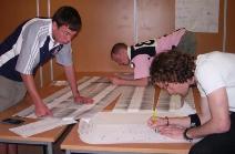
data session - 6/7/2007 - 7/7/2007 Side Scan: Back in the lab the side scan traces were aligned, allowing an overall analysis on the bedform and sediment changes to be made before making a final mosaic of this information combining it with a track plot of our location throughout the day. This was then put onto a poster along with an analysis of the grab contents at each site.
|
||||||||||
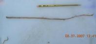
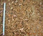 Grab 1 - large grained sediment with dead maerl Grab 1 - large grained sediment with dead maerl
N.B. length of ruler = 17cm
|
Grabs:
(N.B. Latitude and Longitude values are not as accurate
as would be preferred for grab site but more detailed equipment was not
available to us)
|
||||||||||
Conclusion
|
|||||||||||
| Estuarine boats - 9/7/2007 | |||||||||||
|
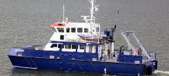
Boats Used: R.V. Bill Conway + R.I.B.
Weather:
Tides:
|
Location:
|
||||||||||
Introduction
 The
overall aim was to investigate the biological, chemical and physical
processes taking place within the Helford estuary. The survey of the
estuary included 5 horizontal cross-transects from the mouth working up
the estuary onboard the RV Bill Conway. In conjunction with this, the
RIB, Ocean Adventure sampled 5 different sites ranging from Gweek Seal
Sanctuary (the closest possible site to the head of the river) to The
Pool (the mid estuary).
At these sites, depth profiles of pH, temperature and salinity were
recorded. Water samples were also taken for dissolved oxygen, phosphate,
silicate, chlorophyll, nitrate and plankton analysis. The secchi depth and velocity
were also taken. The
overall aim was to investigate the biological, chemical and physical
processes taking place within the Helford estuary. The survey of the
estuary included 5 horizontal cross-transects from the mouth working up
the estuary onboard the RV Bill Conway. In conjunction with this, the
RIB, Ocean Adventure sampled 5 different sites ranging from Gweek Seal
Sanctuary (the closest possible site to the head of the river) to The
Pool (the mid estuary).
At these sites, depth profiles of pH, temperature and salinity were
recorded. Water samples were also taken for dissolved oxygen, phosphate,
silicate, chlorophyll, nitrate and plankton analysis. The secchi depth and velocity
were also taken.
|
|||||||||||
Equipment UsedCTD Rosette The CTD Rosette contains many different pieces of equipment used to create a profile through the water profile. On the Bill Conway 2 bottles were fired at each specific depth to ensure a water sample was obtained. Water Sampling Bottles These bottles were fired at defined depths in order to obtain water samples at specific points in the water column. Conductivity On the CTD a conductivity meter is present which measures the conductivity and the temperature. Transmissometer The transmissometer is used to measure the turbidity of the water. It works by sending out a laser signal and received with a narrow field of view measures how much of the energy is received and so determines the transmission, which is wavelength dependant. Fluorometer The fluorometer sends out a series of UV pulses which are absorbed and re-emitted by the chlorophyll within the phytoplankton in the water. The return pulses are detected by the fluorometer and can be used to estimate the amount of phytoplankton present.Niskin Bottles Used in collecting water samples, they are designed for use at variety of depths. A trigger system allows bottle closure once the bottle reaches the desired position in the water column. The bottle is closed via a lid and base, which stay open until triggered, snapping shut upon activation. Trigger systems for bottle closure can be either via a messenger sent down the line, or via an electronic release mechanism. The Niskin Bottles were used on the RIB as a method of collecting water samples. ADCP The Acoustic Doppler Current Profiler (ADCP) is used in the observation and understanding of current flows within the water column. Using multi-directional transducers to send out pulses at a chosen frequency, return signals from the output sound pulses are intercepted and reflected either in the water column or at the seabed. When elements return echoes, they arrive at different times, with the frequency of the pulses being shifted due to Doppler Effect. Sampling over time across and area allows a profile of water currents to be built up. YSI probe The YSI probe is a multi-parameter probe, used to measure pH, temperature, depth, salinity and dissolved oxygen, which can be used on any vessel but here was used on the RIB as it is a simple hand-held instrument which can be deployed over the side by use of a cable and provides lots of information which on the Bill Conway was obtained by use of the CTD. Secchi Disk A secchi disk is a simple piece of low-tech equipment which allows the light penetration through the water column to be observed. The disk has a surface of alternating black and white areas and it is lowered over the side of the vessel by hand until it disappears from sight. The depth at which it disappeared is measure by distance marks on the line, or tape measure, and this depth is a third of the depth of the euphotic zone (the area at which photosynthesis can take place). When using the secchi disk it important to remember to observe the weather conditions as this may affect how far it can be seen, and to always use the same person, or get an average depth from the same people reading the disk as each person may see it at different depths. Plankton Net We used a 200µm plankton net of Duncan & Associates and attached to it was a Hydrokite counter and the net was trawled behind the Bill Conway. The counter was used to evaluate the volume of water passing though the net. The mouth of the net was 50cm wide and attached to the bottom of the plankton net was a bottle in which to collect samples. Two samples were taken, one at the mouth of the Fal estuary and one at the mouth of the Helford estuary, and these samples were analysed in the lab. Conductivity Meter Onboard the Bill Conway there was a handheld digital display & basic probe with sensors for measuring both temperature and salinity and there was a conductivity meter measuring the salinity and temperature of the water passing through the deck pump. The conductivity was also measured by the CTD and the YSI probe on the RIB.Chemical Processes Once the samples had been collected, preliminary chemical preparation was done onboard to ready the samples for lab work the following day. 60ml of water was passed through chlorophyll filters and these filters were placed in 7ml acetone in labelled test tubes. Water samples, which had been passed through the filters, were placed into glass bottles and plastic bottles ready for phosphate, nitrate and silicate analysis. Samples for oxygen analysis were obtained directly from the bottles on the CTD and Manganous Chloride solution and Alkaline Iodide solution reagents were added to fix the samples before the bottles were stored underwater. At 5 locations the surface samples were added to lugar solution to preserve them so that they could be analysed for phytoplankton. When a sample from the zooplankton net was collected it was put into a labelled bottle and formalin was added to preserve the sample. |
|
||||||||||
|
|
Estuarine lab - 10/7/2007ChemistryThe methods used to analyse the samples taken on the boat were standard procedures. The chorophyll, phospate and silicon method were taken from Parsons T. R. Maita Y. and Lalli C. (1984) “ A manual of chemical and biological methods for seawater analysis” 173 p. Pergamon. The dissolved oxygen method was taken from Grasshoff, K., K. Kremling, and M. Ehrhardt. (1999). Methods of seawater analysis. 3rd ed. Wiley-VCH and the nitrate method was taken from Johnson K. and Petty R.L.(1983) “Determination of nitrate and nitrite in seawater by flow injection analysis”. Limnology and Oceanography 28 1260-1266. Biology In the lab we investigated the phytoplankton samples taken and preserved with lugol, and the samples from the zooplankton net. The samples were left overnight and so the plankton was able to sink to the bottom of the bottles/tubes. This meant we were able to decant off the excess solution from the phytoplankton therefore condensing the solution from 100ml to 10ml. This condensed solution was placed in ratchet slides an 1ml of solution was observed and the phytoplankton seen was recorded. The zooplankton samples from the plankton net were agitated and a known volume of the sample was placed in a Bogorov counting tray. The zooplankton species from both samples were observed and recorded. |
||||||||||
|
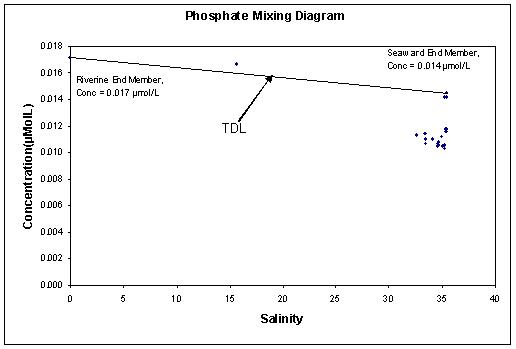
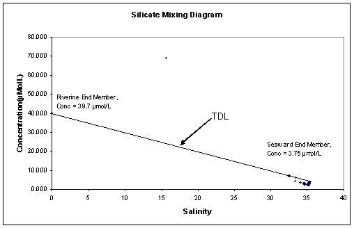
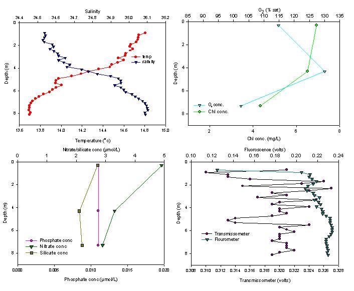
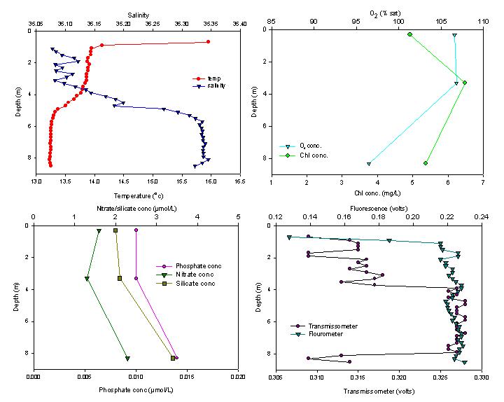
Estuarine analysis - 11/7/2007 Physics ADCP The data resulting from the ADCP onboard the Bill Conway was analysed back in the laboratory using WinRiver playback. From this each transect was re-run and tabulated data was extracted to gain the average velocity. This was then combined with density data from the CTD and inputted into the Richardson’s number equation (see below left): NB. Station 2 was not used in this calculation as the file did not save correctly onboard due to CTD equipment failure. The Ri numbers from station 3,4 &5 were then plotted on to the graph below against depth. If Ri is below 0.25 then mixed conditions exist, if above 1 stratification occurs. The graph shows that all of the flows observed in station 3,4 & 5 are laminar, with a slight increase in turbulence observed in station 3, but not significant enough to make this an actual turbulent flow. Also stations located closer towards the mouth (station 3) have slightly higher Ri values than more inland stations because of the more turbulent conditions caused by the increased shear velocity from the incoming tide, i.e. samples before high tide at 11:56GMT. Stations 4 & 5 were sampled after high tide at 12:04GMT and 12:20 respectively on a slack tide producing the lower laminar flows seen at these areas. Backscatter The transect at station 2 emits a relatively constant amount of backscatter in surface waters, with a few stronger peaks occurring in some areas. (Fig1) Figure 2 shows the backscatter occurring at station 3. The highest backscatter present occurs at surface waters around elapsed time 4 - 6s. The next peak occurs at a depth of 2-3m which may correspond to the thermocline and consequently the chlorophyll maximum. Again there appears to be a rise in backscatter in surface waters, this time arising between elapsed time 122-140s, yet this peak emits less backscatter than the previous surface amount. Overall, Station 4 shows relatively little backscatter. Although some does occur between an elapsed time of 4 & 20s in the surface waters, in comparison to the other stations, this station appears to show the lowest backscatter amounts. (fig 3) Figure 4 shows the backscatter about station 5. There are three points of concentrated backscatter, which is possibly due to high chlorophyll levels. The first area occurs at an elapsed time of 32 and a depth of roughly 2m, which is similar to station 3. The next two regions occur at times 70 & 90s, and both extend from the surface waters to a relative depth of 2m. These readings correspond to high chlorophyll values, at shown by figure 4. Chemistry Nutrients Nutrient concentrations within the Helford generally follow the patterns that would be expected within an estuarine system. From our data, nitrate appears to be conservative in behaviour although a lot more data is required around intermediate salinity values to support this. As our data is largely toward the high end salinity values it is difficult to make assumptions about the estuary as a whole (Fig 5). Phosphate behaves interestingly within the Helford as, assuming our end member concentrations are correct there appears to be massive removal of phosphate at the seaward end of the estuary. However, it is more likely that there is an input of phosphate beyond our estuarine data sites which have caused the seaward end member to appear higher than it would be in reality. It is therefore possible that the TDL should slope more downwards towards the seaward end as phosphate is removed by biological processes within the estuary (Fig 6). Silicate shows non-conservative behaviour within the Helford as the data does not appear to be grouped closely around the TDL between the two end members around S=15 (Fig 7). This could be because of the diatoms within the water column dying and dissolving back into the water column after moving upstream with the tidal influx, producing what looks like an input of organic silica into the water. All three of the horizontal nutrient profile suffer from a lack of data in the upper estuary due to the fact that a large part of the Helford is made up of intertidal zones that we could not access. Vertically, the nutrient profiles change moving up and down the estuary. Towards the head end, nutrient maximums occur in the surface waters and nutrients become depleted with depth (Fig 8). This is probably associated with a high anthropogenic input at this point due to the surrounding farmland. Moving down the estuary, biological processes and physical stratification of the water column lead to the depletion of the nutrients in the surface waters below the levels found higher up and a deepening of the nutrient maximum. This is because nutrients can accumulate below the euphotic zone where they are not utilized by phytoplankton (Fig 9). CTD and YSI The CTD and YSI data taken upon the Bill Conway and the rib also show what would be expected within an estuarine system. The sites furthest upstream show the smallest amount of stratification as the mixing processes associated with the tidal system stop a thermocline from developing (Fig 10). Further downstream, a seasonal thermocline has developed within the water column as well as a halocline formed by the relatively low salinity river water flowing over the more water underneath (Fig 9). However, the salinity differences are roughly 0.3 which is a very low difference between the two water bodies. There is also what appears to be a diurnal thermocline within our data caused by the input of solar energy into the surface waters during the day with diffuse processes not being enough to transfer this energy to depth. This causes the surface waters to increase in temperature. |
|||||||||||
|
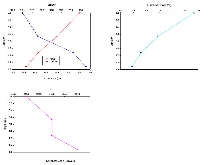 Fig 10
(click to enlarge graphs) |
|||||||||||
| Biology Phytoplankton
Zooplankton
|
|||||||||||
|
|||||||||||
| Offshore boat - 12/7/2007 | ||||||||||||||
|
Boat Used: R.V. Callista Weather:
Tides:
|
Location:
|
|||||||||||||
|
Introduction
The
aim was to investigate the biological, chemical and physical
properties occurring at a front located offshore from Falmouth. A
thermosalinograph was used to observe the location of the front.
Several sites were determined both on the front and offshore and
depth profiles for temperature and salinity were developed.
Water
samples were also taken for dissolved oxygen, phosphate, silicate,
chlorophyll, nitrate and plankton analysis.
|
|||||||||||||
| Equipment Used As on the Bill Conway a CTD, Secchi Disk, ADCP and Plankton Net were used. The equipment was all used in the same way on the Bill Conway with a few exceptions. ADCP The ADCP used on the Callista was similar to Bill Conway and we produced transects at both a resolution of one sample per 1m and also at one sample per 1/2m. Plankton Net The difference between the plankton net on the Bill Conway and the plankton net on the Callista is that on the Callista we sampled the water vertically through the water column whereas on the Bill Conway a sample was taken by means of a trawl of the net behind the vessel. In addition a thermosalinometer was used. Thermosalinometer This is used to continually measure the sea surface salinity and temperature along the track of a ship. It is mounted close to the water intake of the vessel. |
|
|||||||||||||
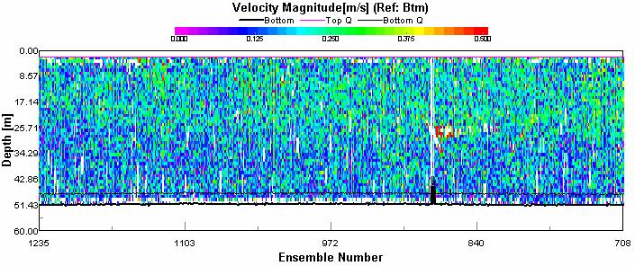 Fig 11
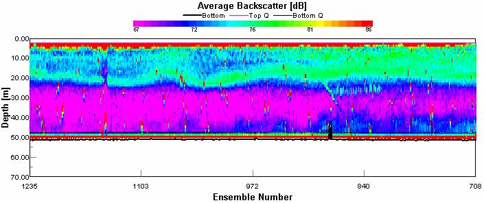 Fig 12
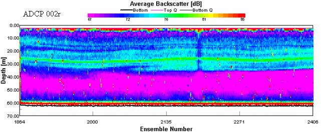 Fig 13
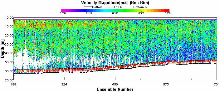 Fig 15
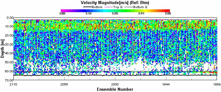 Fig 17
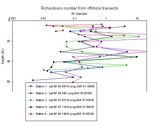 Fig 18
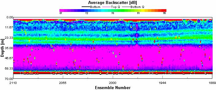 Fig 19
(click to enlarge graphs)
Fig 19
(click to enlarge graphs)
|
Offshore lab - 13/7/2007 The methods used to analyse the data obtained from the samples were the same standard procedures which were used to analyse the samples from the estuarine boat work. The chorophyll, phospate and silicon method were taken from Parsons T. R. Maita Y. and Lalli C. (1984) “ A manual of chemical and biological methods for seawater analysis” 173 p. Pergamon. The dissolved oxygen method was taken from Grasshoff, K., K. Kremling, and M. Ehrhardt. (1999). Methods of seawater analysis. 3rd ed. Wiley-VCH and the nitrate method was taken from Johnson K. and Petty R.L.(1983) “Determination of nitrate and nitrite in seawater by flow injection analysis”. Limnology and Oceanography 28 1260-1266. The phytoplankton was preserved with lugar and were observed under a microscope in a ratchet tray the following day and the zooplankton were preserved with formanin and observed in a Bogarov tube under a microscope. | |||||||||||||
| Offshore analysis - 14/7/2007 Sheltered Site one is located at the mouth of the Fal Estuary, near Black Rock. This site has a prominent shallow thermocline, with nutrient levels increasing with depth. The highest phytoplankton concentrations were found surface waters which can be attributed to the depletion of nutrients in this region. Coastal side of front The water column before the front is well mixed compared to other sites studied, this can be seen in the velocity magnitude plot, figure 1. The average backscatter trace, figure 2, shows a weak seasonal thermocline at approximately 20m deep, this is relatively shallow due to turbulent mixing of the water column. The photic layer above the thermocline is nutrient depleted due to a high level of phytoplankton, primarily diatoms; this may cause the high turbidity seen in the Transmissometer data, (figure 3). High levels of primary production is also inferred due to the O2 saturation levels being above 105%, which is well above levels caused by external factors including wave motion and thus must be due to the production of O2 in photosynthesis. The nutrient concentrations below the thermocline rise as there are lower light levels in the disphotic zone and thus no net photosynthesis to consume them. In the front Approaching the front, the thermocline migrated from a depth of 35m to the surface as shown in average backscatter plot figure 4. Due to the upwelling of nutrient rich deep water at the front, there are high levels of phytoplankton production and companionably there is likely to be high zooplankton densities. This causes high nutrient depletion in surface waters. Within the front the Ri values decrease, therefore the water column becomes more unstable. The stable layer seen at the beginning of the velocity magnitude trace figure 5 diminishes. Seaward side of the front There is an apparent increase in water stability with an increasing Ri no. and a strong picnocline present. O2 concentrations remain high and chlorophyll levels remain relatively low, suggesting that there is much mixing in the surface waters, preventing phytoplankton from remaining in the upper layers for an extended period of time. However, nutrient concentrations all show similar decrease in the surface waters down to the thermocline, proving that it is utilized by phytoplankton. The chlorophyll maximum occurs at the thermocline between 20-25m, as shown by figure 6. This niche would normally be assumed to be inhabited by motile Dinoflagellate species which were able to utilize the deeper nutrient maximum. Nevertheless, upon phytoplankton sampling and identification it was found that the dominant group of primary producers present was in fact Diatoms. The abundant Chaetocerous sp is able to stay at the deeper depths and out-compete Dinoflagellates due to their reduced size and mass. Offshore The velocity magnitude plot figure 7. shows that at approx. 5-20m depth there is a very clear stable layer within which there is a vastly increased velocity. This can also been seen on the Ri graph for the same station, (figure 8), whereby an Ri value of 776.07 is seen at approximately 15.6m depth. It is commonly accepted that if Ri > 1 the column can be said to be stable, values < 0.25 are said to be unstable. It is believed that within very stable subsurface flows called ‘holmboe’ waves can occur and these were observed on our ADCP trace as billows of movement above and below the flow. The average backscatter plot figure 9 shows how this subsurface layer is affecting the biology of the water column. Using this information and that gathered from the phytoplankton counts at approximately 20m there is a large amount of plankton biomass. This, unlike other sites, occurs below the thermocline indicating a deep euphotic layer. At this level, chlorophyll levels have been found to increase by 10µmol/L. After this maxima Silicate and Phosphate increase again because, due to insufficient light levels, the plankton can no longer grow at this depth, thus not utilizing these nutrients. This site also showed the presence of the strongest picnocline of all transects. | ||||||||||||||
| Biology Phytoplankton
Zooplankton
|
||||||||||||||
Conclusion
|
||||||||||||||
| Conclusion Over the past two weeks the physical, chemical and biological properties of the waters surrounding the Falmouth and Helford Estuarine systems have been investigated. In particular the main phytoplankton and zooplankton species, as well as the concentrations of the main nutrients located offshore and inshore were observed. The bathymetry of the sea bed surrounding the Helford estuary has also been studied. The location of the front existing off the coastline has been pinpointed, and through collaboration with other groups it was found that during the current conditions of low riverine input it is situated only a few miles offshore south west from Falmouth. The nutrient concentrations have been shown to be highest at the head of the estuary, and the nutrients behave as expected in the estuarine water column at this time of year; with low concentrations found in the surface waters, increasing to a maximum either at the thermocline or at depth. Also nitrate and turbidity has a pronounced effect on the groups of primary producers present and on the amount/efficiency of primary production. Poor weather conditions have limited data collection on occasion, but the necessary data has been collected for efficient and reliable analysis of the estuarine system. After a recent period of bad weather the inshore and offshore areas were sampled after several days of high irradiance and thus the reestablishment of the seasonal thermoclines has occured. The culmination of the research was the first recording of 'Holmboe' waves below the statified offshore surface layers out of the labratory, as before this they had only been seen in mathematical models. |
| * Weather information taken from Lands End buoy, 62107, off Seven Stones Lightship. Coordinates: 50o69 N, 6o60 W |
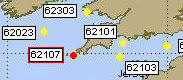 Location of buoy 62107 |
ReferencesHughes S. H., 1999. The geochemical and mineralogical record of the impact of historical mining within estuarine sediments from the upper reaches of the Fal estuary, Cornwall, UK. Spec. Publ. Int. Assoc. Sedimentol., 28, pp 161-168 Fish J.P & Carr H.A., 1990. Sound Underwater Images, Guide to The Generation and interpretation of Side Scan Sonar Data. Lower Cape Publishing. Grasshoff, K., K. Kremling, and M. Ehrhardt. (1999). Methods of seawater analysis. 3rd ed. Wiley-VCH. Johnson K. and Petty R.L.(1983) “Determination of nitrate and nitrite in seawater by flow injection analysis”. Limnology and Oceanography 28 1260-1266. Parsons T. R. Maita Y. and Lalli C. (1984) “ A manual of chemical and biological methods for seawater analysis” 173 p. Pergamon. Pirrie D., Camm G. S., Sear L. G., & Hughes S. H., 1997. Mineralogical and geochemical signature of mine waste contamination, Tresillian River, Fal Estuary, Cornwall, UK. Environ. Geol., 29, pp 58-65 Pirrie D., Power M. R., Rollinson G., Camm G. S., Hughes S. H., Butcher A. R. & Hughes P., 2003. The spatial distribution and source of arsenic, copper, tin and zinc within the surface sediments of the Fal estuary, Cornwall, UK. Sedimentology, 50 (3), pp. 579-595 Rostron D. M., 1985. Surveys of harbours, rias and estuaries in Southern Britain, Falmouth. Nature Conservancy Council, CSD Report, 623, pp. 1-11 National Data Buoy Center; National Oceanic and Atmospheric Administratiion: www.ndbc.noaa.gov/index.shtml |
|
The views opinions and scientific analyses expressed in this website are those of the authors and do not necessarily represent those of the University of Southampton or the National Oceanography Centre, Southampton


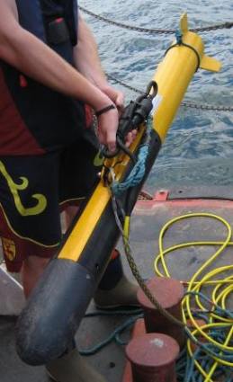 Side Scan Sonar
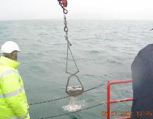
 Grab 1 - polychaete worm
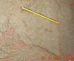 Grab 2 - fine grained sediment
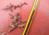 Grab 3 - Live Maerl examples
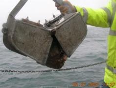 Grab 4 - rock wedging open the
grab
Grab 4 - rock wedging open the
grab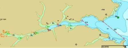
 RV Bill Conway
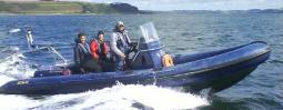 R.I.B. Ocean Adventure
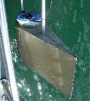 ADCP
ADCP Using the Niskin bottle
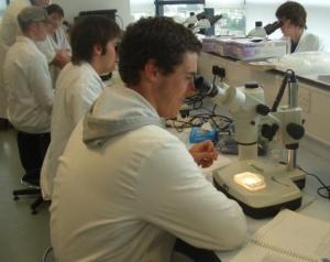 Observing
zooplankton
Observing
zooplankton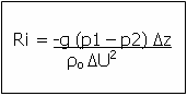 Richardson's number equation
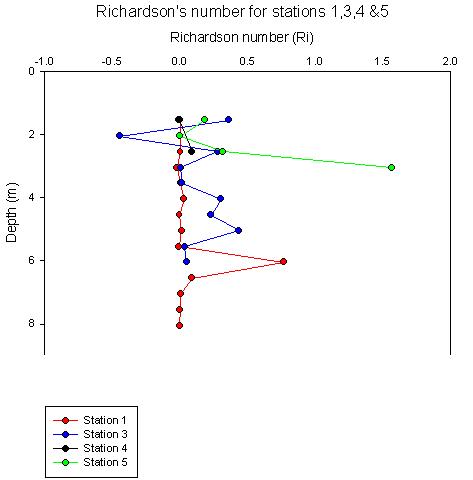


 Working on the
CTD
Working on the
CTD