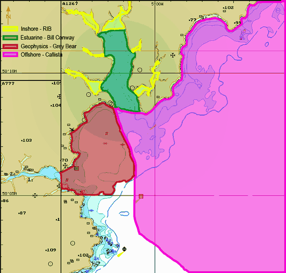
![]()
|
|
|
CONTENTS
|
 |
|
Claire O'Sullivan, Lizzie Chellew, Ross Fairgrieve, Helen Earwaker, Hannah Govan, Louise Sizer, Gareth Lewis, Alistair Henwood, Craig Barrett, James Lawrence |
|
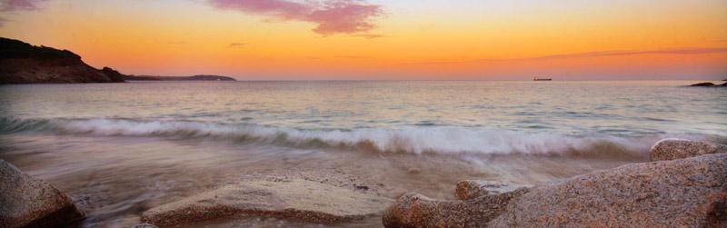
The Fal Estuary is located on the south
west coast of the UK (refer to fig. 1), and is a drowned river valley known as a ria.
The name Fal is old Norse/Danish Viking and dates
from the Viking age. The River Fal is approximately 29km in length, with its
source at Goss Moor near St Dennis, and extends 18km inshore. The deep section
known as Carrick Roads, makes up 80% of the main body of the estuary. It is the
third largest natural harbour in the world and has been a bustling port since
the fourteenth century; now the principal port of Cornwall. The Fal
estuary is macrotidal with a spring tidal range of 5.3m and at Truro it becomes mesotidal with a range of 3.5m. The local geology is meta sedimentary
rocks from the Devonian period, predominantly carnmellis granite, metamorphic aureole and
china clay. The estuary has experienced historical mining dating back to the Bronze Age. The main elements that have been mined are tin, copper, lead and iron, the mining has caused much of the tailing deposited in the Restronguet Creek. This has lead to the creek being the most metal polluted area in the UK. Some species have developed high metal tolerance levels, these species have large metal concentrations in their blood, particularly copper (Cu, which currently exceeds the European Quality Standard, level of 5µml-1). Species equitability is low in Restronguet Creek, with a high dominance of two main species Nereis Diversicolor and fucus vesiculosus. The last mine was closed in 1991 (Wheal Jane), but mine drainage still continues. The abstraction of Maerl still occurs to this day. The area also suffers from other pollution including sewage discharge, antifouling release and material from the docks. The area is a Site of Special Scientific Interest (SSSI) because of the local biological aspects.
|
|
Figure 2: RV Callista |
|
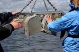
RV Callista RV Callista (refer to fig. 2 and 3) is a 20 metre research vessel owned by the National Oceanography Centre. As well as having a financial value of around one million pounds, the research vessel has unequivocal educational value, providing students with hands on experience in practical oceanographic skills. Being a catamaran, RV Callista is an inherently stable vessel which allows for large payloads to be carried and operated. A large ‘A’ frame on the stern of the vessel is typically used to lower the CTD into the depths and can be used to tow various equipment through the water. Another inbuilt feature is the hull mounted ADCP, which can measure sub surface flows and zooplankton distribution. Data and samples can be analyzed on board in one wet lab and one dry lab.
A state of the art Bridge
allows for excellent visibility on and around the vessel and where there
are blind spots, cameras provide coverage. The skipper has access to Navifisher;
this program incorporates Admiralty Charts, Maximum speed over ground can be as high as 18-19 knots, with bow thrusters mounted in the bow for precision in positioning. The draught of the vessel is approximately 3 metres this allows for relatively good access to inshore sites.
|
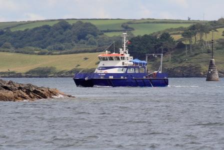
| RV Bill Conway
For more littoral use,
students of the National Oceanography Centre have the option of using an
inshore sampling vessel with a more shallow draught than RV Callista,
yet the capability to handle relatively substantial payloads. RV
Conway's
|
| Ocean Adventure
Ocean Adventure was used for sampling of shallow water
riverine sites, reaching areas that any other research vessel could not
sample.
|
|
MV Grey Bear MV Grey
Bear is a 15m*6m*1m
landing
craft-multipurpose workboat owned by Falmouth Divers
licensed for up to 12 passengers and 2 crew
and despite a painfully slow maximum speed of 7 knots is very useful in
the local inshore The Grey Bear is powered by twin Perkins engines (270 hp) meaning that while she is not fast, the Grey Bear is a highly practical and stable vessel. |
|
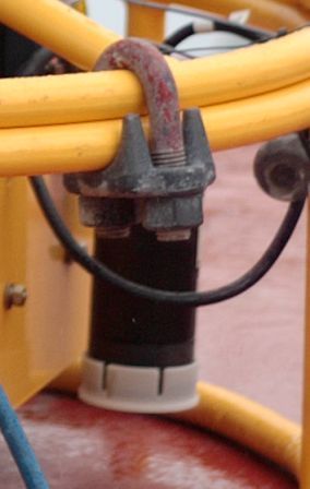
Acoustic Doppler Current Profiler (ADCP) The Acoustic Doppler Current Profiler
is used to measure the speed and direction of currents within the water
column. Multi-directional transducers send out pulses at a chosen
frequency and these pulses are reflected in the water column or at the
seabed.
|
CTD
A
multi parameter platform that is capable of continuously recording
temperature, salinity and depth with a variety of additional instruments
mounted upon a large m
|
|
Niskin Bottles M Niskin bottles can be deployed via a rosette frame (i.e. on board a CTD frame), usually a total of six per frame. On retrieval of equipment, water is drawn of into plastic sampling bottles for further analysis in the laboratory (oxygen, nutrient analysis and taxonomic identification). |
Secchi Disk This is a simple piece of equipment
used for measuring water clarity. It is a disk with a diameter of 20cm
and is split into four quadrants, alternating between black and white.
It is d
|
|
Nets
>Closing Zooplankton
Net: Before the advent of the closing zooplankton net, gaining a sample
of zooplankton at a certain depth in the water >Tow Net with Flow meter: The purpose of this instrument is to measure the amount of water flowing through the measured circumference of the net, and from this the density of zooplankton per cubic metre can be calculated. >Fine Mesh Phytoplankton Net: Used extensively throughout oceanography to collect samples of phytoplankton. Simple and effective however a weight needs to be connected to the tail of the net in order for the mouth of the net to be fully submerged and thus provide a representative sample. |
Fluorometer
A fluorometer provides a measurement of the
co |
| Temperature and Salinity Probe Suitable for in situ fundamental measurement of temperature and salinity variation with depth.
|
Transmissometer
|
|
YSI The YSI probe is a multi parameter probe measuring various factors including temperature, salinity, pH and dissolved oxygen levels. The YSI probe has simple cable deployment to the desired depth (constrained by cable length) and continuous data is sent to a handheld digital readout. It is a compact and easy to use piece of equipment. |
Tow fish
Sidescan sonar is used to locate bathymetric
features and topography. The transducer can be mounted |
| Chlorophyll Fluorometry Parsons T. R., Y. Maita. and C. Lalli. (1984). A manual of chemical and biological methods for seawater analysis. p.173, Pergamon. |
Oxygen Concentration Semi-automated Winkler reagent method. Grassoff, K., K. Kremling and M. Ehrhardt (1999). Methods of seawater anlysis 3rd ed. Wiley-VCH. |
Nitrate Flow injection analysis using spectrophotometry. Johnson K. and R. L. Petty (1983). Determination of nitrate and nitrite in seawater by flow injection analysis. Liminology and Oceanography 28 p.1260-1266. |
Phosphate Spectrophotometry analysis Parsons T. R., Maita Y. and Lalli C. (1984). A manual of chemical and biological methods for seawater analysis. p.173, Pergamon. |
Dissolved
Silicon Spectrophotometry analysis, treated with reagent (ammonia molybdate) and reducing agent (MRR; Metol Sulphite : Oxilic Acid : Sulphuric Acid : MQ Water, 10:6:6:8 respectively) Si(OH) 4 + 12 MoO4 = + 24 H+ -> H4SiMo12O40 + 12 H2O(reaction after adding the reactant) Parsons T. R., Maita Y. and Lalli C. (1984). A manual of chemical and biological methods for seawater analysis. p.173, Pergamon. |
|
Calibration Checks YSI 600 Serial Number F105C These calibration checks show the errors for the YSI probe for temperature and salinity. Temperature Checks Standard: SBE 35 Serial No: 37 Salinity Checks Standard: P147
FSI CTD These calibration checks show the errors for the CTD equipment used. Temperature Checks
Conductivity Checks High bath:
Low Bath:
Pressure Checks:
|
| Figure 4: Offshore Route Click to enlarge |

|
Aims and Objectives Aims:
Objectives:
|
|
General Overview Offshore data collection occurred on the RV Callista on the 5/7/07 from 07.47GMT to 14.45 Low tides at 02.33 GMT (1.1m) and 14.49 GMT (1.2m). High tides at 08.26GMT (4.8m) and 20.34 (5.1m). Weather conditions: in the morning south westerly to southerly wind direction, force 4-5. In the afternoon this changed to south westerly to westerly winds of force 5-7, and occasionally 8. Visibility of 2 nautical miles. Raining periodically, anti-cyclonic conditions with a low pressure system over us. i.e. very windy and very wet! After a short briefing on safety we decided to change our original course due to inclement weather conditions. This was to ensure that the work being done further offshore was completed before the winds increased in the afternoon. At 08.36 GMT we departed from the pontoon and headed to station 1 at Black Rock. At this location we did our first transect across the mouth of the Fal estuary and collected our first samples using the CTD and plankton nets. At station 2, samples were collected with no problems so it was straight on to station 3 once our work had been carried out. Station 3 however, was a different story; our second transect was to be started here but, due to the bad winds it was decided that carrying out a second transect would not provide us with any useful data, the ADCP was also showing that the water column was highly mixed and was almost identical to station 2 so we decided not to collect any water samples. We also had a surprising fire alarm here so we all had to vacate our posts and assemble to the fire point to have a role call (thankfully all were present). Once we had arrived at station 4, we were able to carry out our sampling taking as planned as was the case with station 5. After all the 5 stations were completed, we arrived back at shore at 14.45GMT wet with wind hair. |
| Chemistry Lab
From the Niskin bottles samples were taken at various stations to determine the concentration of dissolved oxygen, nitrate, phosphate, dissolved silicon and chlorophyll. and to identify phytoplankton and zooplankton species. The water samples were dispensed into individual bottles, i.e. plastic for silicon concentration, glass for the other nutrients, and were refrigerated until further analysis was under taken in the laboratories. Dissolved Oxygen The first water samples collected were used for oxygen saturation analysis. The samples were fixed with 1ml manganous chloride and 1ml alkaline iodide respectively. Nutrients: Nitrate Silicate & Phosphate 50ml of seawater was taken up using a syringe and after a syringe filter added. Through this10ml was then flushed; giving 5ml into each plastic silicon bottle and 5ml into the brown glass bottles for the nutrient samples. This first 5ml was discarded and a further 40ml was added to the brown glass bottles. Another 50ml of seawater was taken up and a new syringe filter was attached. 5ml was discarded to flush the filter and then 10ml was added to the brown glass bottle making up the total 50ml sample used for nitrate and phosphate analysis, and 35ml was added to the plastic bottle for the silicon analysis. Chlorophyll From the syringe filters, the filter papers were removed and folded in half using forceps. Each filter was placed in 7ml of 90% acetone making sure it is fully submerged and then stored in a cool box until transferring into a laboratory. Plankton 100ml was syringed from the water sample and stored in plastic screw top bottles. |
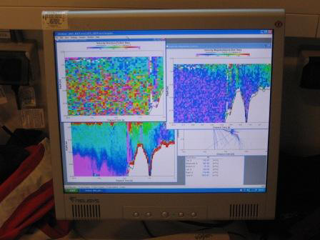
| Computers In order to track the CTD progress through the water column we used the software package CTDave to obtain live feedback from the equipment. Niskin bottles on the CTD rosette were triggered from within the boat electronically at the desired depths. The ADCP recorded the current profile at each station and the velocity magnitude. A new technological addition on the Callista was the thermosalinograph. This was used to record the underway temperature and salinity of the water and was refreshed every 30 seconds throughout the survey. Unlike the ADCP, which requires a slow vessel speed, the thermosalinograph can produce profiles at higher cruise speeds. |
|
CTD Data
At station 1 (fig. 5) the temperature changed from a maximum of 13.04ºC at the surface to a minimum of 12.58ºC at a depth of 25metres (m), showing a difference of 0.46ºC. This change is very small and suggests a lack of a strong thermocline. Chlorophyll increased to a depth of 8.13m, and steadily decreased with depth to a minimum concentration of 1.36µgL-1. The extracted chlorophyll data from the water samples was 2.9µgL-1 at 2.5m and 1.36µgL-1 at 25.30m respectively. The extracted chlorophyll data supports that from the CTD probe and indicates that the chlorophyll maximum (3.58µgL-1) is at a depth of 8.10m. The data from the transmissometer decreases from the surface (3.78) to around 10 m (3.73), then, increases to 3.77 at 16.11m, before declining to the minimum value of 3.72 at a depth of 25.40m. The original decrease in the transmissometer data was due to the phytoplankton presence at the corresponding depth in the water column. However, as the transmissometer data decreased from 16.00m to 25.40m in tandem with the chlorophyll levels, the data suggests there is a presence of suspended sediment from the estuary which might be responsible for the aforementioned change in values. The LUP data presented a linear decrease with depth as one might expect, and the Secchi disk results for station one highlighted the euphotic zone, the near-surface layer in which light is sufficient for net photosynthesis (Miller, 2004), at a depth of 16.50m (fig. 10). The nitrate values were higher at 25.30m (7.09µmolL-1) than at the surface reading of 2.50m (5.22µmolL-1). Phosphate values were higher (1.43µmolL-1) in the 25.30m sample than at the surface sample taken at 2.50m (0.41 µmolL-1). This difference is due to nitrate and phosphate being utilised by the phytoplankton for successful growth in surface waters. Station 2 (fig. 6) showed a decrease in temperature from the surface reading of 12.89ºC at 1.03m to 12.68ºC at 18.90m, again lacking evidence of a developed thermocline. Chlorophyll increased from the surface to a maximum of 3.01µgL-1 at a depth of 4.24m, and then generally decreased to a depth of 19.00m. The extracted chlorophyll sample data was 3µgL-1 at 2.20m, 3.12µgL-1 at 3.60m, and 1.36µgL-1 at 18.50m respectively, supporting the CTD chlorophyll values. The transmission data decreased from the surface to a minimum of 3.74 at 3.20m, then increased over the next 6.00m to a maximum of 3.82 (9.40m). Transmission was lowest when chlorophyll values were highest due to the likely presence of phytoplankton in the surface 5.00m. After its peak, transmission decreased with depth and with chlorophyll concentration, again indicating the presence of sediment suspended in the water column, this is perhaps due to the shallow depth and proximity of the station to the coastline. The weather conditions and subsequent physical mixing of the water column on the day of sampling could have also affected the suspension of sediment. Again as expected the LUP data decreased linearly with depth from a maximum of -0.12V at 1.00m, to a minimum of -0.28V at 18.86m. The Secchi disk data indicated the euphotic depth to be at 18.00m for station 2. Nitrate and phosphate values were lowest at the surface (4.72µmolL-1 for nitrate, 0.5µmolL-1 for phosphate), where chlorophyll was highest, as they are depleted by phytoplankton. At both stations 1 and 2, silicon values were relatively uniform throughout the water column.At station 4 (fig. 7), the temperature decreased with depth from 13.18ºC at the surface to 12.1ºC at 50.00m depth. Station 4 demonstrated a clear thermocline at around 20-25m with a temperature change of 0.80ºC. Chlorophyll data closely followed the pattern for temperature decreasing from 13.2µgL-1 to 1.0 µgL-1 over 7m. The extracted chlorophyll values supported the CTD data, and indicate the chlorophyll maximum (14.9µgL-1) to be at 12.10m. The Secchi disk results implied that the euphotic depth was 13.50m. The data from the transmissometer showed an increase with depth in the same way that temperature and chlorophyll decreased with depth. A minimum value of 3.16 was present at the surface and only indicated a significant increase after 20m. This low transmission was due to a high abundance of phytoplankton above the thermocline, and was supported by the low nutrient levels. The transmission then increased to a value of 3.97 at the bottom of the thermocline, and remained steady for the remainder of the downcast. This uniformity in the data indicated minimal presence of plankton and suspended sediment below the thermocline. LUP was not included in the offshore stations (stations 4 and 5) due to the LUP data becoming erratic with increasing depth. The nutrient levels increased with depth, as they are replenished by upwelling and mixing of the lower water column. The data for station 5 (fig. 8) is more erratic thus making it difficult to see clear trends, due to the deteriorating weather conditions at the location. As expected, temperature decreased with depth from a maximum of 12.63ºC at the surface to 12.45ºC at 19.50m. This small change did not suggest the presence of a strong thermocline. Chlorophyll increased from 5.60µgL-1 at 0.58m to its maximum (6.85µgL-1) at a depth of 9.00m, and then decreased steadily to a value of 2.80µgL-1 at 19.50m. The extracted chlorophyll data was 6.05µgL-1 at 3.00m and 6.85µgL-1 at 9.00m, which indicated the chlorophyll maximum and supported the CTD data. The Secchi disk results showed the euphotic zone to be at a depth of 13.50m. The transmission data increased from 3.60 at the surface to 3.80 at 19.50m, indicating the presence of phytoplankton in the surface water, and minimal suspension of sediment or plankton in the lower water column. The concentration of nitrate decreased from surface levels (3.84µmolL-1) to 3.35µmolL-1 at 9.06m, and phosphate also decreased from 6.60µmolL-1 at 2.96m to 2.55µmolL-1 at 9.14m. Again, this is likely due to utilisation by phytoplankton, however, the nutrient levels at this station are much higher compared to station 4 due to the chlorophyll levels, an indirect measure of phytoplankton activity, being lower.
Equipment Error and Calculations The CTD was calibrated against a standard temperature (refer to calibration section), and the probe had an error of 0.02ºC; and against a standard salinity of 11.42 and 32.60 there was an error of 0.02 and 0.18 respectively. To convert fluorescence into chlorophyll the extracted chlorophyll samples were plotted against fluorescence (fig. 9) and linear regression (R2=98%) was used to produce the following equation: y=0.41x + 0.73. |
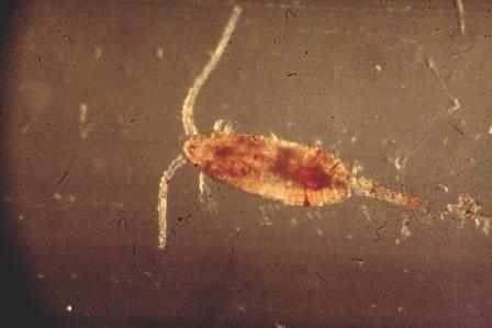
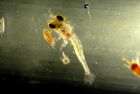
| Plankton A closing plankton net was used onboard Callista to collect water samples from various depths at stations 1, 2, 4 and 5 to allow for the taxonomic analysis of phytoplankton and zooplankton in the offshore Fal. Some species found have not been included in the graphical analysis due to very low abundance.
For each site (except site 3) a closing plankton net was deployed, the results of which are shown in the pie charts. The charts show that Copepods (fig. 11) make up the majority of each community, ranging from 52% to 97% of the total zooplankton population. There is approximately one Copepod per litre of water in each sample. At site 1, positioned at Black rock, the water was well mixed and the plankton net was deployed from 6 metres to the surface. In this sample there is a high proportion of copepods. Decapod Larvae (fig.12) made up 3.70% of the total population and Copepod Nauplii 5.56%. The chlorophyll levels at site 1 (fig.13) were low, ranging from 1.4-3.6µmolL-1, this implies that the phytoplankton population was too low to sustain a high diversity leading to one species dominating in this case the Copepods. The Copepods are successful due to their ability to modify their diet over a wide range of food sources. The Site 2 (fig.14) sample proved to be almost completely composed of Copepods making up 97% of the zooplankton community in this sample, once again the low chlorophyll levels suggest a low phytoplankton population, with chlorophyll at this site being even lower than that at site 1 (1.5-3.0µmolL-1). Site 4 (fig.15) was the only site with an evident thermocline (a change of one degree Celsius), it was also the furthest offshore, thus leading to high levels of chlorophyll (chlorophyll maximum was 14.90µmolL-1). Here the net was raised from 26m to the surface and turned out to be the most diverse location, due to the high phytoplankton numbers leading to a greater diversity as there was a high availability of food; with 11 groups other than Copepods present and copepods making up only 52.61% of the organisms present. Site 5 (fig.16) was well mixed and, like site 1, had comparatively high proportions of Copepod Nauplii (6.59%) and Decapod Larvae (1.32%). The Copepods still proved to be the dominant group with 88.79% of all organisms found being from their order.
At station 1 (fig. 17) the diatom Chaetoceros was the most abundant phytoplankton species (87% at 2.5m; 99% at 25m), followed by the diatom Rhizosolenia delicatula. At station 2 samples were taken from three different depths (fig. 18). Like station 1, Chaetoceros dominated the phytoplankton throughout the water column (77% at 2.2m; 89% at 5.6m; 35% at 18.5m), but a more diverse population could be seen at the deepest sample (18.5m). The results from station 4 (fig. 19) identify Chaetoceros as the most abundant phytoplankton species (92%) at 6m but was absent at 47m. At this depth the diatom Rhizosolenia delicatula occupied 32% of the population sampled, with four other phytoplankton species (Nitzschia, Mesodinium rubrum, Rhizosolenia setigera, and Ceratium fucus) each accounting for 17% of the community. At a depth of 3m at station 5 (fig 19), the dominant species were Thalassiosira rotula and Rhizosolenia delicatula (34% each) followed by Chaetoceros (30%). At 9m, Chaetoceros once again dominated the community accounting for 84% of the four diatom species found. Diatoms clearly dominate the phytoplankton communities in the offshore and mouth of the estuary, as only 2 species of dinoflagellate were found in the four samples (at station 2 and 4). The most abundant diatom was Chaetoceros, which appeared to bloom in shallower waters, as it was scarce or absent from deeper samples offshore. At these depths (i.e. 47m at station 4) other phytoplankton species were dominant suggesting that they are out competed by the chained (and therefore more buoyant) diatom Chaetoceros in surface waters. As expected, total phytoplankton abundance was greater in the surface water column down to the bottom of the euphotic zone, where nutrient (in particular silicon, required by diatoms), and light levels are high enough to support a phytoplankton population.
|
|
Conclusion
Overall five stations were set out to be surveyed but samples were only taken at four of the stations due to a lack of scientific interest at site 3 as well as a formal safety drill interrupting the station. This lead to only one significant thermocline being established at the furthest offshore station (station 4), however the information gathered was still valuable. Phytoplankton levels were highest at station 4 with a strong thermocline and low surface nutrients. Unfortunately the front was not located possibly due to the cooler and less settled weather conditions this summer pushing the front further offshore than previous years. |
| Figure 20: Route Map of Transects on Grey Bear |

|
Aims:
Objectives:
|
| Figure 21: MV Grey Bear |

|
General Overview The geophysical data was collected onboard the Grey Bear (fig. 21) using a Side-Scan Sonar and a Van Veen Grab on the 9/07/07 from 08.49 BST to 15.30 BST. Low tides at 05.52 (1.5m) and 18.24 GMT (1.7m) with high tide at 11.56 (4.5m). Weather conditions were bright with intermittent cloud cover. Wind direction was north to north-westerly at 13mph increasing in the afternoon. Air temperatures ranged from 12-17°C with good visibility all day. After
being transported from the pontoon out to the Grey Bear we set off
towards Falmouth Bay to undertake transects using side-scan sonar
for Natural English. Six transects were completed spanning the
lengths of Gyllyinvase
|
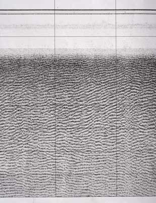
| Onboard Science Using a side-scan sonar (towfish) with a 150 metre swath and 500khz power (high frequency, giving greater attenuation yet better resolution) we set out to map Falmouth Bay. The data was sent back to ship via a cable to a computer where these data were processed. One computer showed the boat’s passage and the plotted transect lines; another, the data readings from the tow fish. The side-scan tracer printed out the findings in real time. Due to the GPS antennae and the towfish having different positions, we measured the distance between them, the distance from antennae to stern of the boat plus the length of the tow cable attached to the fish, to work out the layback. Layback results in a slight time delay between the GPS data and the side-scan, the main computer allows and corrects for layback. Another issue (not very important for our data) is that one transmitter on the towfish was at a different amplitude from the other. On the side-scan print out times are given every 30 seconds in AST. Bification was seen, the splitting of ripples, this is a good sign of wave generated ripples (rather than tide generated ripples). Sediment dynamics were seen to be quite energetic, giving quite mobile living conditions, perhaps suggesting low populations of sessile organisms. In the onshore lab the ripples will be measured and grain size can be estimated as 1/1000 of the ripple size. Therefore wider ripples suggest coarser grain sizes. At the start of every line the ‘main event’ button on the tracer was pressed and SOL (start of line) or EOL (end of line) with line number was notated on the trace. Buoys and boat passage close to our survey were also noted to avoid confusion later in analysis (buoy effect on surface waters are picked up and can look lie bedforms). The towfish uses piezoelectric crystals which pulse and contract which controls the sound and shape. The length of the trace depends on boat speed and whether travelling with or against the current, stretching or compressing the trace.
|
| Interpreting the
Side-Scan Data
The information gathered
on the Grey Bear was collected on many metres of paper, this data
required interpretation. The first part of interpreting this data
was to roll out the sheet containing the scan transects on it, and
cut them into segments for each transect; leaving a gap at the
beginning and end of each transect to account for distortion caused
by the boat turning. After this the separated transects were
aligned with each other in the
At each point the time must be noted and the depth of the water we were in, we get this by measuring from the centre of the paper record to the first solid return. We divide this number by the width of the paper from the centre to the edge and then multiply the result by swath width to get the depth of water. E.g. distance to first return = 2cm, therefore depth = (2/15.15)*75= 9.9m.
Next we need the distance to the boundary directly from the fish, this is found by measuring the distance from the bed to the centre of the paper record. Then we divide this by the representation of swath width and multiply it by swath width, e.g. distance from bedform to centre of the paper = 6.1cm, therefore direct distance = (6.1/15.15)*75= 30.2m. Finally we can use these 2 values and Pythagoras theorem to work out the distance from the fish to the bedform across the sea bed, e.g. using the values above, 30.22-9.92= 814.03. √814.03= distance across sea bed from fish to boundary=28.5m. After doing this for all the boundaries they can be plotted on the Northings and Eastings plot to produce a map of the bedforms.
|
|
Bedforms The Side-Scan Sonar records show that large areas of our survey contain megaripples. These ripples have an average wavelength of 1.34m and amplitudes of 0.13m decreasing to 0.075m towards the shore. These are generally all long waves with relatively small amplitudes; this suggests that they have been created over long time scales. The majority of these waves have a plan pattern sinuous in phase. Offshore the ripples are likely to be affected by currents predominantly flowing in a constant flow direction. The tide sweeps round Falmouth Bay on both the flow and the ebb of the tidal cycle, this is caused by the shape of the local coastline. This flow occurs as the tide goes in and out of the English Channel, driven by the amphidromic point just outside the Solent. Storm waves are multidirectional on reaching the shallower water of the shore line. Our inshore section of our survey had a depth of 8-9m, shallow enough for storm waves to be possible. This explains why the ripples found have decreased in amplitude. Towards the shore the sediment becomes finer, but has a greater shell content. This creates a coarser bulk property of the sediment, making it more difficult for ripples to be initially formed. |
| Grab Samples Van Veen grab samples were collected at 4 sites in Falmouth Bay and the biota and sedimentology were analysed on deck.
|
|
Summary Large areas of megaripples were found becoming smaller towards the shore. This coincides with the changing bulk sediment properties and shallowing of the water depth. Although dominated by megaripples and flattened bedforms, outcrops of rocks were also found, protruding from a local headland. There were few definitive boundaries between the different bedforms. A large amount of maerl was found, but the majority of this was dead, making up the main component of the sediment. The greatest amount of living organisms, mainly echinoderms and molluscs, were found at grabs C and D, both on the flatter bedform.
|
| Figure 36: showing transects and stations completed on July 12th |

|
Aims and Objectives Aims:
Objectives:
|
| General Overview: The Estuarine practical was carried out on the 12th July 2007. The team was split into two groups; seven members aboard the R.V. Bill Conway and three members aboard the Ocean Adventure Rib. Weather conditions remained constant throughout the day, being 15°C-17°C with 8/8 cloud cover (no rain). The conditions were calm with low winds from the NE. The R.V. Bill Conway left docks at 9.30GMT and headed up the estuary as far as Truro River where it became too shallow to continue; with low water occurring at 9.38GMT. Five transects were carried out. CTD downcasts were used at the sites of the transects and water samples were taken where required. The first transect was undertaken at the confluence of the Truro and Fal rivers. A CTD downcast led to water samples being taken at 0 metres and 7 metres. The second transect was conducted across the River Fal by Smuggler’s Cottage. The third transect taking place downstream near Tolcarne Creek. The fourth traversed the main channel at Pill Point. The fifth transect taking samples along the Falmouth Harbour Limit near Mylor. The Ocean Adventure rib departed Falmouth docks at 09:34 GMT heading upstream to Malpas Point on the Truro River. Water samples were taken at five stations to measure a range of nutrients along the estuary, working downstream on the flood tide. A YSI multi-probe was also deployed to study the parameters of the water column (temperature, salinity, pH, turbidity, chlorophyll & oxygen saturation). At station 3 a zooplankton net was towed for 5 minutes at 1 knot. The net deployed had a mesh size of 200µm.
|
| CTD data: Rib
Site 1 (fig. 37) was located at Malpas Point, which is the highest point up the estuary that was sampled. The water column was very shallow so only the surface 1m was sampled using a YSI probe. Probably the most interesting variable in the surface metre was salinity which increased by 5. The chlorophyll maximum was found at the surface and decreased with depth, along with turbidity, as expected. Temperature also decreases with depth by 0.2˚C as you would expect to find in the water column due to higher light levels and solar heating at the surface. O2 saturation increases with depth, however the results from the YSI probe are not of considerable significance as only 2 samples were taken throughout the water column. Site 2 (fig. 38) was sampled further down the estuary over 6m with samples taken every metre. Temperature decreased by approximately 2˚C over 6m displaying a relatively linear profile. Salinity showed a significant increase of 12 in the surface 2m and then increased to 34 in the lower 4m. Chlorophyll concentration decreases with depth suggesting a higher level of biological activity in the surface metre where light levels are highest. The turbidity profile supports this data as it also decreases with depth. The results for O2 saturation displays a lower percentage at the surface 2m, which is a questionable result, as you would expect the saturation to be higher at the surface due to turbulent mixing and high chlorophyll concentrations. The profile below 2m supports the result we would expect to find. The results from site 3 (fig. 39) present a more variable profile when considering chlorophyll concentrations and turbidity, suggesting that the water column is becoming less stratified. The temperature and salinity profiles are similar to site 2 with less saline, warmer water at the surface. The O2 saturation displays the same anomalous result as site 2, with a lower saturation in the surface 2m, where you would expect there to be a higher saturation. Once again, the profile from 2-5m displays the expected results. Site 4 (fig. 40) located further down the estuary show very similar profiles to site 3. Temperature decreases with depth, while salinity increases with depth. The chlorophyll concentrations are highest at the surface, decreasing by 2.0μgL-1 over 10m. Turbidity is also highest at the surface, following the profile you would expect considering the changes in chlorophyll concentration. As with sites 2 and 3, the results for O2 saturation are questionable in the surface 2m, and support the expected percentages in the lower 8m. The results for site 5 (fig. 41) show an increase in salinity and a decrease in temperature with depth, as you would expect. Chlorophyll concentration increases with depth to a maximum of 6.4μgL-1, but turbidity displays an unexpected result with higher levels where chlorophyll concentrations are lower. You would expect there to be lower turbidity where chlorophyll levels are lowest due to fewer particles in the water column. This result is therefore questionable for this station. O2 saturation shows the expected result below 2m but also displays the same anomaly as the previous three sites. Bill Conway
Along transect 1 (fig. 42) the temperature gently decreased from a maximum of 16.3°C at 1m depth to a minimum of 14.6°C at 6.7m presenting a change of 1.7°C. The salinity along the transect increased from 23.4 to 29.0 in the first metre and then gradually increased to a maximum of 32.9 at 6.7m. The chlorophyll concentrations were variable along the transect, with a minimum value of 8.12 μgL-1 at 2.7m and 4.3m and a maximum concentration of 9.65μgL-1 at 1.5m and 6.7m. This variability reflects a considerable amount of background ‘noise’ in the estuary. ‘Noise’ is also detected in the surface metre of the water column as can be seen in the results from the transmissometer. As would be expected, opacity in the surface few metres is highly reduced, perhaps due to floatation and suspension of sediment. Transmission largely increases in the surface 3m to a value of 0.09V and remains fairly uniform to 6.7m. Transect 2 (fig.43) was carried out further down the estuary towards the mouth from the surface to a depth of 11m. Temperature followed a similar profile to transect 1, decreasing gradually from a maximum of 16.3°C at 1m to a minimum of 13.7°C at 11m. The salinity profile increases by 7.6 in the surface 2.5m, and then gradually increases to 34.7 at 11m depth. Chlorophyll concentrations are less variable compared to transect 1, displaying a large increase from 4.2μgL-1 – 10.0μgL-1 in the surface 2m, then gradually decreasing to 6.2μgL-1 at the deepest point. This appears to make sense when considering the tranmissometer results, light drops rapidly from 4 metres and chlorophyll levels also drop considerably at this point. This indicates that the increasing absorbance of light the water is the cause for the decrease in phytoplankton. Transect 3 (fig. 44) displays many of the same characteristics of transect 2 however there are notable differences in some of the data. According to the tranmissometer results the sediment load appears to be comparatively higher at the surface, however as previously mentioned the root cause of this may be the increased chlorophyll concentrations in the surface waters. The fact that the tranmissometer readings show an increased water clarity when chlorophyll concentrations decrease at approximately 3 metres. The salinity at the surface is still relatively low while deeper waters have increased salinity (i.e. values upwards of 32). However this stratification is visible in all transects. Along transect 4 (fig.45) the temperature decreased by a relatively large amount in the surface 4m, from 15.3°C to 13.9°C, then dropped again to a minimum of 13.6°C in the bottom 9m. The salinity profile follows a similar trend to the other transects with a large increase in the surface 4m. Chlorophyll concentrations also follow a similar trend, with a large increase in the surface 3m to the chlorophyll maximum (2.5μgL-1) then decreases as expected with depth, as light decreases. Transmission is lower in the surface waters where you would expect the water to be more turbid, then increases slowly with depth, as the water becomes clearer. Transect 5 (fig. 46) was carried out closest to the mouth of the estuary, the salinity profile indicates a more mixed water column of higher salinities compared to the other transects carried out further up the estuary. Temperature decreases with depth as expected from 15.1°C at the surface to 13.2°C at 22m. Chlorophyll concentrations show the same trend across the mouth of the estuary with a large increase in the surface 5m to the chlorophyll maximum (18.5μgL-1), and then a slow decrease with depth. Considering this, transmission increases with depth due to decreasing chlorophyll levels and suspended particles in the water column. Conclusion The overall trends display a decrease in temperature down the estuary towards the mouth as the estuary becomes deeper. Salinity increases down the estuary as it mixes with more saline water from offshore. This correlates with the temperature decrease observed as mixing activity increases. Higher chlorophyll concentrations found lower down the estuary indicate greater biological activity and a more diverse community. This correlates with depleted nutrient concentrations. O2 percentage saturation is expected to be higher at the surface due to turbulent mixing and biological activity, but the results show an anomaly in the surface 2m for each station. The deeper sections of the profiles support the result we would expect. |
|
ADCP: Transect 1
Start Position: 50o 13.669N, 005o 00.930W End Position: 50o 13.660N, 005o 00.989W Start Time: 1056GMT (52 seconds long) – 1hr 32 mins after low water. Transect Length: 76 metres This transect was made from the left to the right bank of the River Truro, approximately 200 metres from its mouth. There is a very slow upstream (northerly) flow ranging in velocity from close to 0ms-1 to approximately 0.2ms-1. This is the expected result as this transect was carried out only 93 minutes after low water resulting in low velocities in the upstream direction. Transect 2
Start Position: 50o 13.258N, 005o 01.506W End Position: 50o 13.254N, 005o 01.649W Start Time: 1124GMT (92 seconds long) – 1hr 50 mins after low water. Transect Length: 165 metres This transect ran from the left to the right bank of the Fal, just South of Lamouth creek. There was a general upstream (northerly) movement of water caused by the flooding tide. The average tidal velocity from the surface to approximately 7 metres (m) depth was approximately 0.08ms-1 with a faster average velocity of around 0.3ms-1 occurring from 7m to the bed. This result is expected as the seawater entering the estuary on the flooding tide is more saline and therefore has a higher density than the out-flowing river water. This means that the northward velocity peaks in the deeper parts of the transect, as the majority of the more highly saline water flows up-estuary beneath the fresher river water. Freshwater input from the higher reaches of the Fal is likely to have been contributing to the slower velocities in the upper 7 metres. The increase in average current velocity over transect 1 is also expected as this transect was carried out 18 minutes later and the flooding tide therefore had more of an effect. This station is also further downstream meaning that less tidal energy will have been dissipated at this point than at the site of transect 1. Transect 3
Start Position: 50o 12.400N, 005o 01.777W End Position: 50o 12.492N, 005o 01.836W Start Time: 1150 GMT (93 seconds long) – 2hr 16 mins after low water. Transect Length: 184 metres This transect also ran from the left to the right bank, just upstream from Tolcarne and Channals Creeks. The general direction of flow was, again, upstream (easterly). There is a peak in velocity below 4m with an average velocity of approximately 0.3ms-1. Above this the velocity is slower at an average of around 0.1ms-1. There is another area of higher velocity close to the right-hand bank between 2m and 6m. In this area, the average velocity is again approximately 0.38ms-1. Local current direction also varies greatly and this complex pattern of flow is likely to be due to the complicated bottom topography at the bend just down-river from this transect site. Transect 4
Start Position: 50o 12.175N, 005o 02.281W End Position: 50o 12.180N, 005o 02.538W Start Time: 1211 GMT (178 seconds long) – 2hr 37 mins after low water. Transect Length: 299 metres Transect 4 was carried out from the left to the right bank close to Turnaware Point and Pill Point. Once again, the current is moving in an upstream (northerly) direction. The current velocities are fairly uniform throughout the channel with slightly higher speeds in the centre (approximately 0.3ms-1) than at the channel edges (approximately 0.2ms-1). This is likely to be due to friction having less of an effect in the deeper water. It can also be noted that the overall average velocity is slightly higher than the previous transects due to deeper water and later sampling leading to an increase in tidal currents. Transect 5
Start Position: 50o 10.614N, 005o 02.520W End Position: 50o 10.946N, 005o 01.623W Start Time: 1253 GMT (524 seconds long) – 3hr 19 mins after low water. Transect Length: 1201 metres The final transect was made from the right to the left bank between Penarrow Point and Messack Point. The average velocity is higher still than transect 4, being over 0.3ms-1. The area of highest velocity is in the centre of the deep channel where the effect of bed friction is the least. The area of slowest velocity occurs in the shallow area to the east of the deep channel, possibly as a result of deflection from Messack Point.
|
|
Nutrient mixing diagrams:
Each nutrient was plotted against salinity, in a nutrient mixing diagram. It was decided only to use data for nutrient concentrations that was taken at the surface of the water column. This ensures that we are considering the same body of water, for all the results. There were three different ways that salinity could be measured onboard the Conway, the CTD and two T/S probes, one hand held and one developed into a pump continuously taking measurements. The most reliable source was decided to be the CTD and so we extracted the salinity values from that profile. Therefore, the surface samples were not used due to no CTD data. Further salinity data was collected onboard Ocean Adventure, nearer the head of the estuary, using a YSI probe. To eliminate differences between these instruments calibration data was used. The difference between the CTD values and the YSI probe was 0.16 salinity units. Dissolved Silicon (fig.37) As expected the silicon concentration values decrease with distance away from the head of the estuary. The river end member was 86.2µmols/l, where there was a salinity of 0. This is significantly higher than any silicon value that we encountered in the estuary. At the marine end member much lower dissolved silicon values were found at 2.2µmols/l. The range of values that we found where all in the high salinity range of 23 to 35, giving much lower silicon values than if we had progressed up into the river. The values show conservative behaviour, with a fairly even spread of values either side of the theoretical dilution line (TDL). For the results found below the TDL, comparisons were made between chlorophyll concentration and dissolved silicon. This was to consider a possible relationship between the removal of silicon and the production of diatom tests. However, this was not conclusive as the chlorophyll concentrations were considered too low. At the mouth of the estuary moving offshore during spring diatom blooms, lower silicon values would be expected, as they have siliceous cells. Nitrate (fig.38) This shows very conservative behaviour. All the values were close to the TDL, suggesting a relationship between nitrate removal and addition within the system. There is a suggestion of some depletion of nitrate nearer the mouth of the estuary, where greater volumes of phytoplankton are found utilising this nutrient. An anomalous point was also located at a salinity of 27.2 with a nitrate concentration of only 18.3µmol/L. This is discussed further on. Phosphate (fig. 39) The phosphate values show a very wide spread above the TDL, indicating an input of phosphate into the estuary. This is displayed as non-conservative behaviour perhaps caused by sewage being brought up the estuary on the flood tide, by a plant near the Fal estuary mouth. Local agriculture could also be an additional source of phosphate. The values found may be the result of multiple inputs of phosphate at varying levels and subsequent utilisation by phytoplankton communities, capitalising on these higher phosphate concentrations. This affect may not be evident in the nitrate or silicon results as higher natural levels will mitigate the effect of anthropogenic input. Anomalous Results There is an anomalous value seen on all three graphs at a salinity of 27. This was perhaps due to technical problems with the equipment in measuring the salinity value. A possible reason for this is a bottle mis-firing and therefore the sample taken at the wrong depth. The lowest salinity was found at the point where the Fal and the Truro rivers meet. Samples were found to be lower at this point, than further up the Truro River. This would imply greater freshwater runoff from the Fal River. The salinity value where the rivers met was 23.2, however all stations taken along the Truro River were higher, ranging from 28.18 to 30.38. |
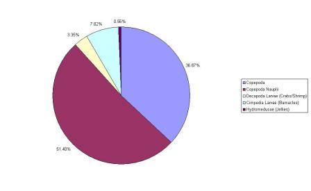
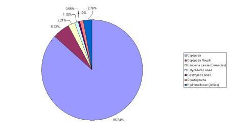
| Plankton: Zooplankton: The zooplankton data collected on the Ocean Adventure (fig. 41)and RV Bill Conway (fig. 40) show a visible difference in organisms between the two samples. The Ocean Adventure sampled the upper estuary using a plankton net towed at the surface by the boat. In the sample collected the most abundant group present was copepods (86.74% of organisms in the sample) at this site the chlorophyll readings were quite low (4.5-6.4µmolL-1) this might explain the dominance of copepods in the area as they are cosmopolitan feeders. Other groups present in quantity include Copepod Nauplii (5.52%), Cirripedia larvae (2.21%) and Hydromedusae (2.76%). Further down the estuary at Carrick Roads the RV Bill Conway collected a zooplankton sample using a Bongo net towed behind the vessel. In this sample the highest proportion of organisms present were Copepod Nauplii (51.4%) followed by Copepods (36.87%) and Cirripedia larvae (7.82%) at this site the chlorophyll readings were far higher, the chlorophyll maximum was at 18.5µmolL-1 and this may have allowed a greater diversity of groups to become established in this area. At both sites the number of organisms counted was lower than that sampled in the offshore work with approximately 1 Copepod for every 3-5 litres of water.
Phytoplankton: Figure 42 shows the total percentage of the different phytoplankton species cells per litre of water. The phytoplankton sample collected on the rib at a depth of 1 metre shows that four different phytoplankton species were present with Chaetoceros sp. (a diatom) being the dominant species in this sample (89%). Three of the four species identified within the sample were diatoms with Alexandrium a species of dinoflagellate making up 3% of the total abundance. The sample taken at station 1, on the RV Bill Conway, composed of five different phytoplankton species. The dominant species at this site were Chaetoceros sp. which comprised of 85% of the total phytoplankton sampled. Alexandrium, a species of dinoflagellate was identified with a total of 1% of the total phytoplankton abundance. Four of the five species identified belonged were diatoms. Station 3 showed the highest species diversity with six different phytoplankton species all of which were diatoms with Chaetoceros sp. being the dominant species with 76% of the total abundance. Station 5 showed the smallest amount of species diversity with only three different phytoplankton species present all being diatoms. The most dominant species present was Chaetoceros sp. with 96% of the total phytoplankton abundance. The diatom species Nitzschia longissima was only found at the three stations sampled using the RV Bill Conway and not found at any of the other stations sampled using either the rib or the RV Callista.
|
|
The Fal Estuary and corresponding offshore area provided a wide range of data from a physical, chemical, biological, and geophysical background. Offshore provided a series of problems, the weather conditions were poor leading to difficulties in gathering accurate and reliable data and hindered efforts to locate the offshore front. It is believed that the front has been pushed further offshore this year, due to a lack of prolonged heating of the water column, and increased freshwater input from the estuary; thus reducing the salinity and temperature properties of surface waters and therefore creating a destablising effect on the stratification near shore. The estuarine-offshore system was analysed by comparing the data collected during both surveys, (estuarine and offshore). The estuary increased in salinity towards the mouth of the Fal as it mixed with more saline water offshore, nutrients also decreased down the estuary towards the mouth due to mixing with seawater together with chlorophyll. Falmouth Bay highlighted how the majority of the sediment within the Fal area is likely to be composed of dead maerl. The transmissometer data from the estuarine sampling suggests that there is minimal suspended particulate matter (SPM) and this can be explained by the dead maerl being too dense for re-suspension. The grab samples from Falmouth Bay provided encouraging signs of benthic diversity within the sample area. From the four grabs 19 individuals were identified to at least a class and some organisms remained unidentified. If possible further investigations are required to fully understand and appreciate the dynamics of the Fal Area. |
Grassoff, K., K. Kremling and M. Ehrhardt (1999). Methods of seawater anlysis 3rd ed. Wiley-VCH.
Johnson K. and R. L. Petty (1983). Determination of nitrate and nitrite in seawater by flow injection analysis. Liminology and Oceanography 28 p.1260-1266.
Langston, W. J., B. S. Chesman, G. R. Burt, S. J. Hawkins, J. Readman and P. Worsfold (2003). Site Charecterisation of the South West European Marine Sites. Fal and Helford c SAC, Marine Biological Association 8.
Parsons T. R., Maita Y. and Lalli C. (1984). A manual of chemical and biological methods for seawater analysis. p.173, Pergamon.
www.soton.ac.uk/noc


 The return pulses will vary in frequency due to Doppler shift
and the frequency change gives a measure of current velocity and
direction. By repeated sampling of the return echo and by gating the
return data in time, the instrument can produce a profile of water
currents over a range of depths. Backscatter can also be used to observe
layers of dense zooplankton populations.
The return pulses will vary in frequency due to Doppler shift
and the frequency change gives a measure of current velocity and
direction. By repeated sampling of the return echo and by gating the
return data in time, the instrument can produce a profile of water
currents over a range of depths. Backscatter can also be used to observe
layers of dense zooplankton populations.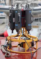 etal framework. Typically a number of Niskin
bottles surround the framework which can be individually and
electronically fired at any depth. Normally a fluorometer is a standard
instrument found on board the CTD which measures phytoplankton density.
Some models of the CTD have a transmissometer which can measure the
transparency of the water at a certain depth through beam attenuation coefficients.
etal framework. Typically a number of Niskin
bottles surround the framework which can be individually and
electronically fired at any depth. Normally a fluorometer is a standard
instrument found on board the CTD which measures phytoplankton density.
Some models of the CTD have a transmissometer which can measure the
transparency of the water at a certain depth through beam attenuation coefficients. ost widely used scientific bottle in the
world. Bottles of various sizes are used for collecting water samples at
a variety of depths. Each bottle may be closed using a simple trigger
system (a messenger is released down static line or via an electronic
release mechanism). The bottles are closed whilst ascending due to
problems involved with pressure increase with depth.
ost widely used scientific bottle in the
world. Bottles of various sizes are used for collecting water samples at
a variety of depths. Each bottle may be closed using a simple trigger
system (a messenger is released down static line or via an electronic
release mechanism). The bottles are closed whilst ascending due to
problems involved with pressure increase with depth.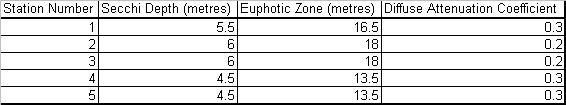 eployed on a line and lowered into the water column. When the
black and white quadrants can no longer be differentiated between by an
observer at the surface, the “Secchi depth” (Zs) has been
reached. The one percent light level (and hence the base of the euphotic
zone) can be estimated as three times the Secchi depth. The diffuse
attenuation coefficient (Kd) can be estimated as 1.44 divided
by the Secchi depth.
eployed on a line and lowered into the water column. When the
black and white quadrants can no longer be differentiated between by an
observer at the surface, the “Secchi depth” (Zs) has been
reached. The one percent light level (and hence the base of the euphotic
zone) can be estimated as three times the Secchi depth. The diffuse
attenuation coefficient (Kd) can be estimated as 1.44 divided
by the Secchi depth.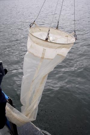
 ncentration of chlorophyll indicating the biological variability and
abundance in the water column. It works by emitting light at one
wavelength, causing the phytoplankton to fluoresce and give off a small
amount of light at a different wavelength. The fluorometer quantifies
light from the phytoplankton, which is converted to a measurement of
chlorophyll.
ncentration of chlorophyll indicating the biological variability and
abundance in the water column. It works by emitting light at one
wavelength, causing the phytoplankton to fluoresce and give off a small
amount of light at a different wavelength. The fluorometer quantifies
light from the phytoplankton, which is converted to a measurement of
chlorophyll.


 and Swanpool beaches. During the transects we
decided on our potential grab sites at 7 different stations using
the trace print out and later collected them with a Van Veen grab.
These varied in composition from the first consisting of mostly dead maerl and broken fragments of shells, to a collection of brittle
stars, an eel fish, many bivalves and an assortment of worms. Having
completed four grabs at stations 1, 2, 3 & 6 we motored back in to
the docks and were ferried back onto the pontoon via Bill Conway.
and Swanpool beaches. During the transects we
decided on our potential grab sites at 7 different stations using
the trace print out and later collected them with a Van Veen grab.
These varied in composition from the first consisting of mostly dead maerl and broken fragments of shells, to a collection of brittle
stars, an eel fish, many bivalves and an assortment of worms. Having
completed four grabs at stations 1, 2, 3 & 6 we motored back in to
the docks and were ferried back onto the pontoon via Bill Conway.


