 |
Falmouth Field Course 2007 University of Southampton School of Ocean and Earth Science
GROUP 5 Chris Evans, Daniel Donnai, Orestis Hartsiotis, Diva Amon, Simeon Archer, Laura Daniels, Oliver Jewell, Matthew Jewers Kwok-Ying Lee, Louis Skelton, Melanie Froude
|
||||||||||||||||||||||||||||||||||||||||||||||||||||||||||||||||||||||||||||||||||||||||
|
|
|||||||||||||||||||||||||||||||||||||||||||||||||||||||||||||||||||||||||||||||||||||||||
|
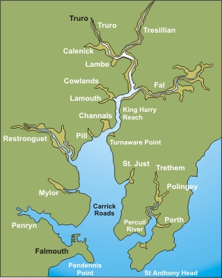
Introduction The Fal estuary is located on the south coast of Cornwall, in the south west of England. This 18km long estuary was formed at the end of the last Ice age when sea levels rose and drowned the river valley creating a Ria. The Penryn, Percuil, Carnon, Truro, Tresilian and the Fal are the six main tributaries of this estuarine system. The main water body of the estuary is known as Carrick Roads. Mean tidal range at spring tides is around 5m with the maximum tidal currents below 2 knots. The mean sea surface temperature is 16˚C in summer and 9˚C in winter. The terrain surrounding the Fal estuary is comprised of granitic rocks to the north and Devonian carboniferous rocks to the west. Rias are important areas for marine life due to the varying range of habitats found along the length of the estuary. These consist of extremely sheltered mudflats found at the riverine end of the estuary to the wave exposed rocky open-coasts found around Shag rock. Unusually, all the habitats found in the Fal area are marine due to the low levels of riverine input. The Fal estuary and the surrounding coastline are a Special Area of Conservation candidate. This is partly due to the presence of extensive rare maerl beds. The Fal estuary is also host to a thriving shellfish industry which is occasionally threatened by blooms of dinoflagellates (red tides). This can cause Paralytic Shellfish Poisoning and is a result of increased metal and nutrient inputs. The Fal estuary is a ‘Sensitive Area’ under the Nitrate Directive. Mining has been a dominant anthropogenic feature of the surrounding area since the Bronze age with peak extractions occurring during the 19th century. The metals previously mined consist of tin, copper, lead, iron, arsenic, tungsten, uranium and silver. The Fal estuary is the most metal polluted estuary in the United Kingdom. The last mine, Wheal Jane, closed in 1991 but the effects of acidic drainage can still be seen. Most metal pollution enters the Fal estuary via Restronguet Creek. Copper concentrations exceed the Environmental Quality Standard (EQS) values of 5ug/l for saltwater. Falmouth is the third deepest natural harbour in the world and as a result has high commercial and recreational usage. The numerous marinas, docks and hence, boats have resulted in high concentrations of organic chemicals such as various antifouling agents and hydrocarbons. Tributyl tin still exceeds Environmental Quality Standards of 2ng/l and causes imposex in dogwhelks and morphological changes in shellfish such as mussels and oysters. This chemical was banned on boats below 25m since 1987 and remaining boats in 2008. Dredging and excessive sewage discharges have caused disruption in the estuary ecosystem as well. From the 3rd to the 14th July, Southampton University’s Oceanography department of 2nd year students conducted a three part survey of the Falmouth and Helford estuarine system and the surrounding offshore area. The aim of this survey was to create a picture of the processes and systems occurring in these areas, keeping in mind some of the above issues.
|
|||||||||||||||||||||||||||||||||||||||||||||||||||||||||||||||||||||||||||||||||||||||||
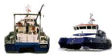
CallistaSpecification
Length overall 19.75m
|
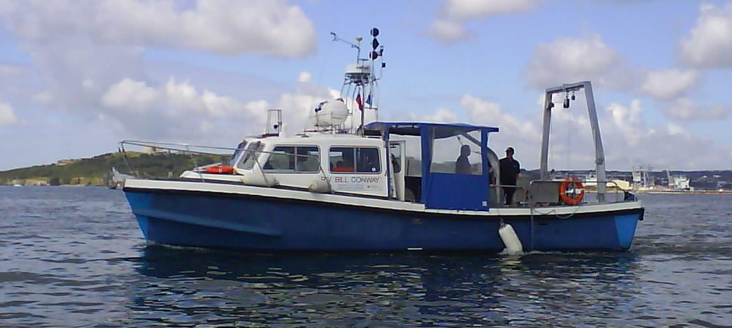
RV Conway
Specification
|
||||||||||||||||||||||||||||||||||||||||||||||||||||||||||||||||||||||||||||||||||||||||
|
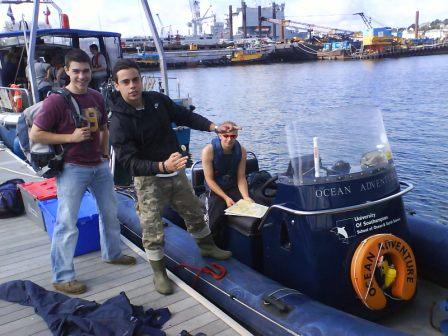
RIBS
Specification
|
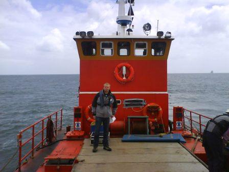
Grey BearSpecification
Dimensions: 15m x 6m x 1.1m
|
||||||||||||||||||||||||||||||||||||||||||||||||||||||||||||||||||||||||||||||||||||||||
|
Equipment Used Throughout The Falmouth Field Course Secchi Disc
Van Veen Grab
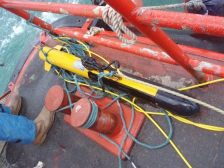
YSI ProbeThe YSI multi-probe is used to measure a variety of parameters, these include temperature, salinity, depth (pressure), dissolved oxygen concentration (in percent saturation and as a physical quantity, mg/l), Chlorophyll (using a flurometer) and turbidity (with a backscatter sensor). Data is collected at 1 second intervals. The probe is compact and easy to employ, making it favourable for use on smaller vessels like the rib. It can be lowered to the desired depth, limited by cable length. Information is displayed on a handheld digital readout, which displays the changing data from the sensors mounted in the probe, in real time.
CTD
ADCP- Acoustic Doppler Current ProfilerAn ADCP is used to measure current flows across the entire water column, using sound. ‘Pings’ are transmitted from transducers at a constant frequency. As the sound waves travel, they ricochet off particles suspended in the moving water, and reflect back to the instrument. A sound wave has a higher frequency, or pitch, when it moves to you than when it moves away, known as the Doppler shift. Sound waves that hit particles far from the profiler take longer to come back than waves that strike close by. By measuring the time it takes for the waves to bounce back and the Doppler shift, the profiler can measure current speed at many different depths with each series of pings. ADCP can be either mounted on an attached rig at the side of the vessel such as on Conway, or as a hull-mounted array, such as on Callista.
|
|||||||||||||||||||||||||||||||||||||||||||||||||||||||||||||||||||||||||||||||||||||||||
|
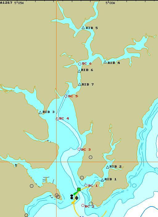
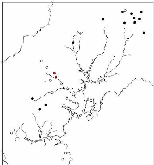
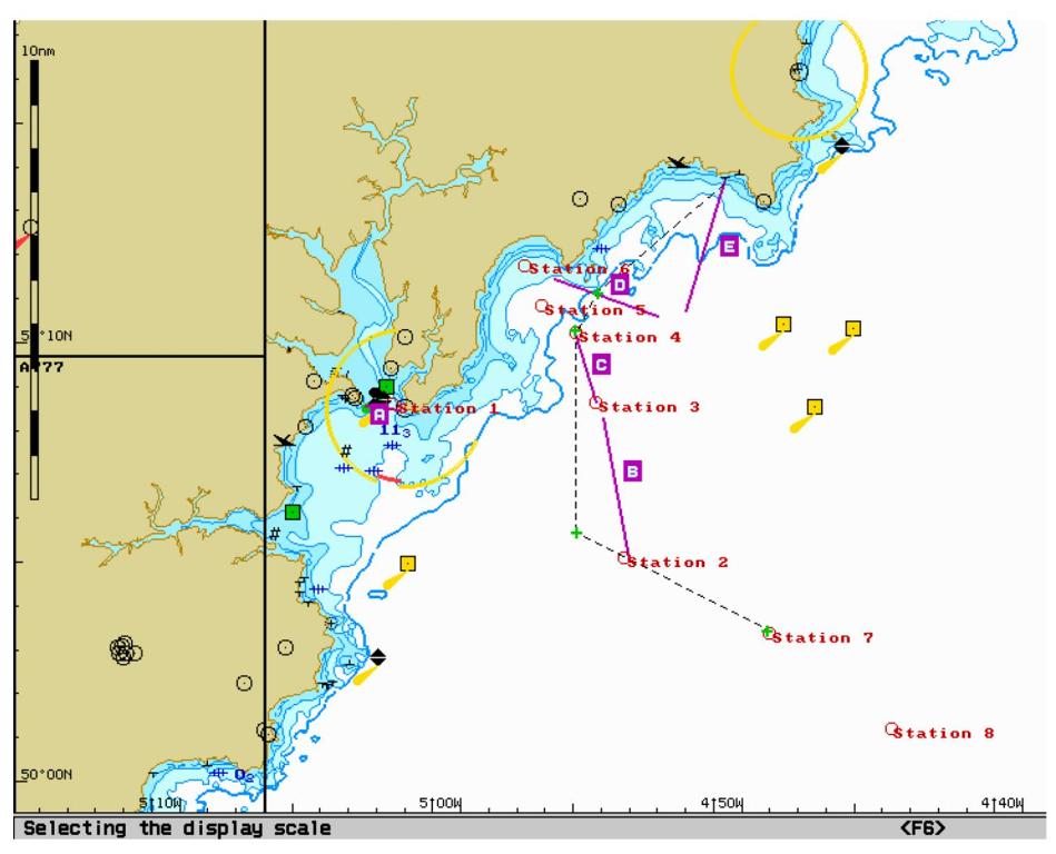
Figure 1. map of stations sampled by Bill Conway and Rib
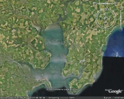
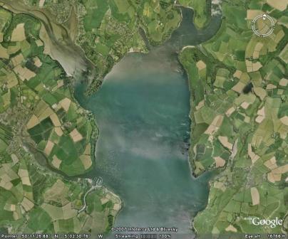
figure 2 aerial images of Carrick Roads and Restronguet Creek. Introduction
The aim of the practical was to analyse estuarine properties, such as physical parameters i.e. temperature and salinity. The chemical conditions within the estuary were also studied, with particular focus on the theoretical dilution of silicates, nitrates and phosphates. Chemical factors will also be linked to the biology within the estuary. This included the phytoplankton and zooplankton community structure and their horizontal distributions within the estuary.
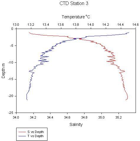
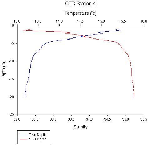
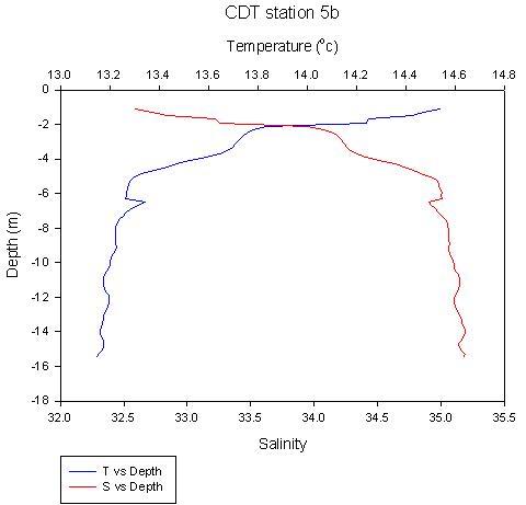
Table 1 conditions on the estuarine study Equipment used A hull-mounted Acoustic Doppler Current Profiler (ADCP) was used to analyse the physical properties within the estuarine water column on the R/V Bill Conway. The group used this device to monitor water density and velocity and hence varying water currents. The ADCP was used for a total of 8 transects. A 6 Niskin bottle rosette was deployed to gather estuarine water samples which were later analysed for chemical studies (Oxygen Saturation, Chlorophyll, Silicate, Nitrate and Phosphate concentrations). The rosette was also used as a frame for a CTD apparatus (Conductivity / Temperature / Depth) which was deployed 7 times throughout the day. A plankton net with a mesh size of 200 µm and a diameter of 50cm was trawled behind the vessel at a depth of 1-2 m for approximately 3 minutes. Equipment onboard the RIB consisted of a YSI probe. This measured Depth, Salinity, Temperature, Chlorophyll, Turbidity, Oxygen Saturation (%) and pH. Plastic bottles were used to store silicate and chlorophyll samples as well as zooplankton samples for the study of community structure. Glass bottles were used to store Phosphate and Nitrate samples. Methods The survey started close to the mouth of the Fal estuary, at the entrance to Mawes estuary. At Station 1, the R/V Bill Conway deployed the CTD at the same time as the RIB deploying the YSI probe. This was done to give an idea of any discrepancies between the two sensors. Sampling was carried out up the main estuary using the R/V Conway whereas the RIB was used to survey shallower upstream tributaries of the Fal estuary.
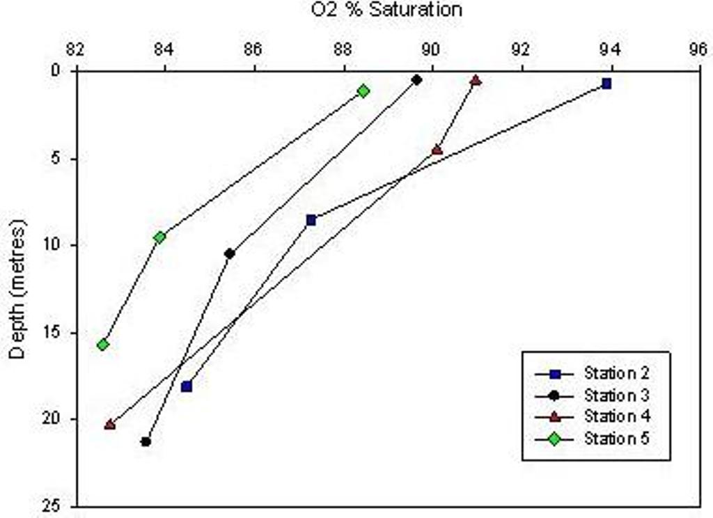
Oxygen Saturation Relationships
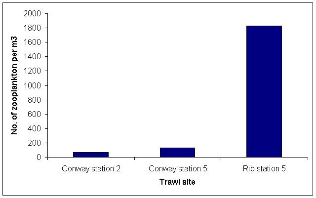
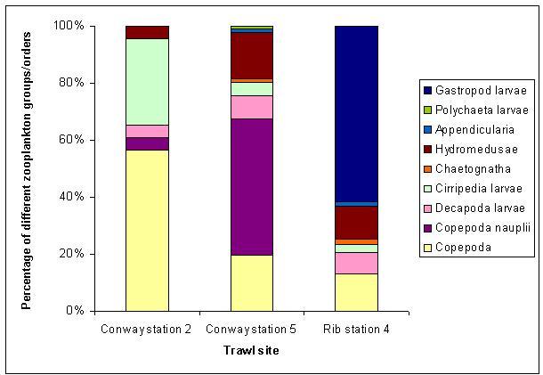
Zooplankton analysis
Phytoplankton
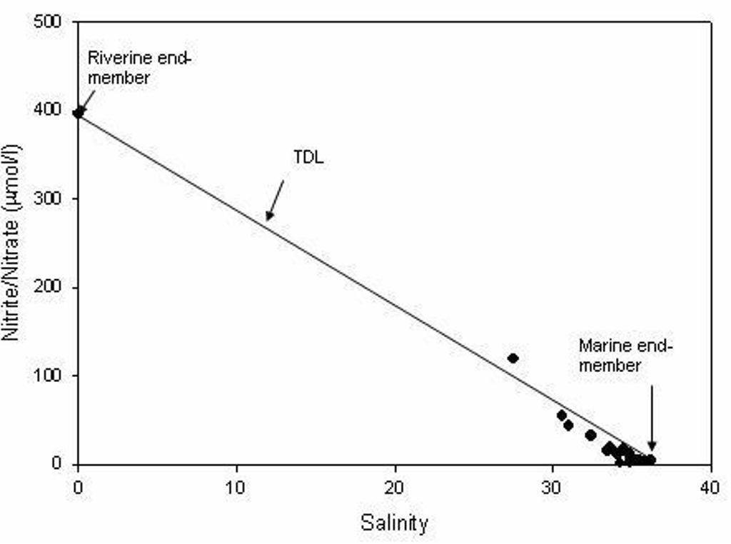
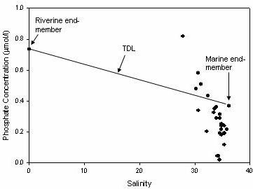
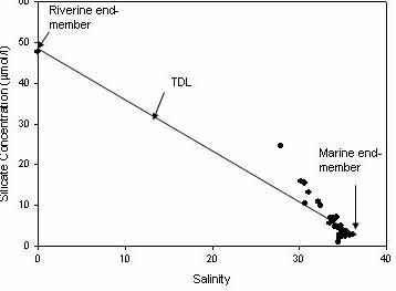
Chemical behaviour Theoretical Dilution Lines
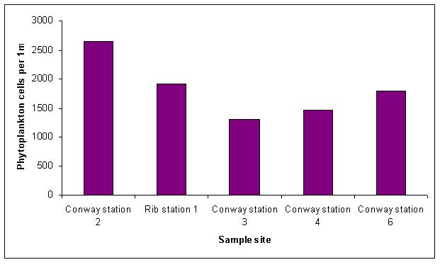
Fig 19a, b & c. Change in nutrients with salinity. Each graph is annotated with a theoretical dilution line between the riverine and marine end-members. (a) Nitrate (b) Phosphate (c) Dissolved Silicon Samples collected around the mouth of the estuary; Conway station 2 and rib station 1, showed high numbers of phytoplankton cells with values of 2640 cells/ml and 1920cells/ml respectively. Conway station 3 around the mid-estuary shows decreased numbers of 1305cells/ml, with an increase again further up the estuary and into the Fal River (1460 and 1790cells/ml respectively). The rib sample contained large numbers of Diatom species, at this station the average Silicate concentration was found to be 7.02mmol/l, this high value correlates with the high number of Diatoms. Station 3 and 4 average nutrient concentrations were low, station 6 however showed an average nitrate concentration of 19mmol/l and a silicate concentration of 6.93mmol/l. Despite the high abundance of phytoplankton and the mouth of the estuary (Conway station 2), nutrient concentrations here are low, however the secchi depth at this station was 6m. The secchi depth decreased with stations further up the estuary, where nutrient concentrations increased. Phosphates, silicates and nitrate/nitrite samples collected from the Bill Conway using Niskin bottles at each sampled station, were analysed in the lab to determine their concentration. Respectively, each major nutrient was then plotted against salinity to graphically establish whether there was a conservative or non-conservative relationship.
Graphs for silicate and phosphate show similar results but to a different extent. There appears to be a small net addition of silicate into the estuary, particularly towards the riverine end-member (fig 19c). This is most likely coming from the weathering of rocks and clay due to heavy rainfall and its associated terrestrial run-off and the re-suspension of bottom sediments and sediment pore water. There is also a small removal of silicate at the estuary mouth due to its utilization by local diatom populations in their development of siliceous shells.
Phosphates show a stronger gradient between addition towards the riverine end-member, and then removal at the estuary mouth (fig 19b). The addition is most likely due to anthropogenic inputs both point and diffuse. Point inputs include sewage outlets, discharges from industrial sources such as detergents, and cage fish farm installations. Diffuse sources include a small amount of terrestrial run-off from the agricultural use of fertilizers (Langston et al., 2003). The effect of this run-off is less significant for phosphate than for nitrate as phosphate is less soluble and tends to remain in the soil for a longer period of time. The high removal of phosphate at the mouth of the estuary is most likely due to the large populations of phytoplankton found within the euphotic zone at this location.
When nitrate/nitrite concentrations were plotted against salinity values there was a strong positive correlation with the Theoretic Dilution Line (TDL) (fig 19a). This means that there is a conservative relationship with a limited weighting towards addition or removal of this nutrient, and any movement of this macromolecule throughout the water column is in accordance to simple dilution and mixing processes. Nitrates and nitrites are therefore removed by photosynthesis and added via the same processes as that for phosphate.
As continuous sampling was not carried out towards the riverine end-member there is a break in the data series. For the nitrate/nitrite relationship with salinity this is not an issue as the behavior is clearly conservative. However, for the relationships involving silicate and phosphate against salinity there can be two explanations. Firstly, conservative behaviour may arise due to weak river input. The second and more likely reason is due to the area having numerous river inputs and therefore more than one riverine end-member.
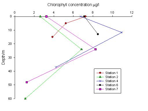
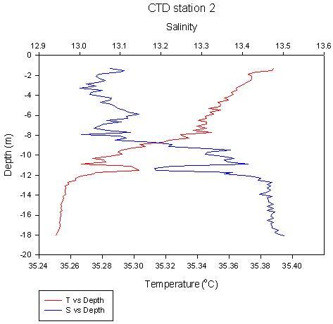
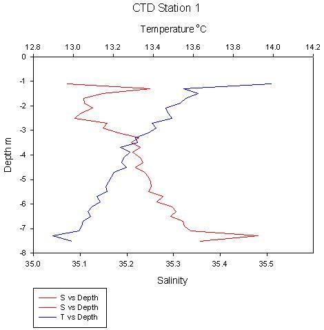
Nutrient Depth Profiles The first cast was taken at the mouth of the Percuil River. Casts 2 to 6 were taken in order from the mouth of the estuary towards the head. All samples showed stratification. In samples 1, 2, 3 the chlorophyll maximum was at the thermocline. In samples 4, 5 and 6 the chlorophyll concentration was similar at the thermocline and at depth. Chlorophyll levels at the thermocline ranged from 4.33 to 5.33µg/l, with highest values in cast 2 and lowest values in cast 1.
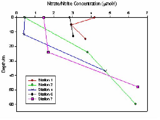
Figure 20. Nitrate/Nitrite plotted with depth at stations 1 to 6.
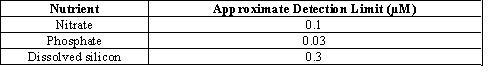
As per table 2 the Nitrate samples are above the detection limit. Nitrates showed lowest concentrations at the mouth of the estuary and then increased with progression up the estuary (figure 20). This was as expected as Nitrates showed conservative behaviour. Samples at depth and at the thermocline for casts 1 to 5 were relatively similar. Surface samples decreased in concentration from the cast 6 to cast 1 due to dilution. High current flows were seen at the sample 6 site which may account for the increased level of nitrate/nitrite due to increased inputs from the river.
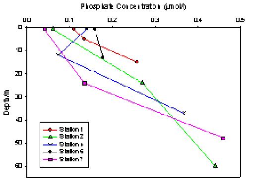
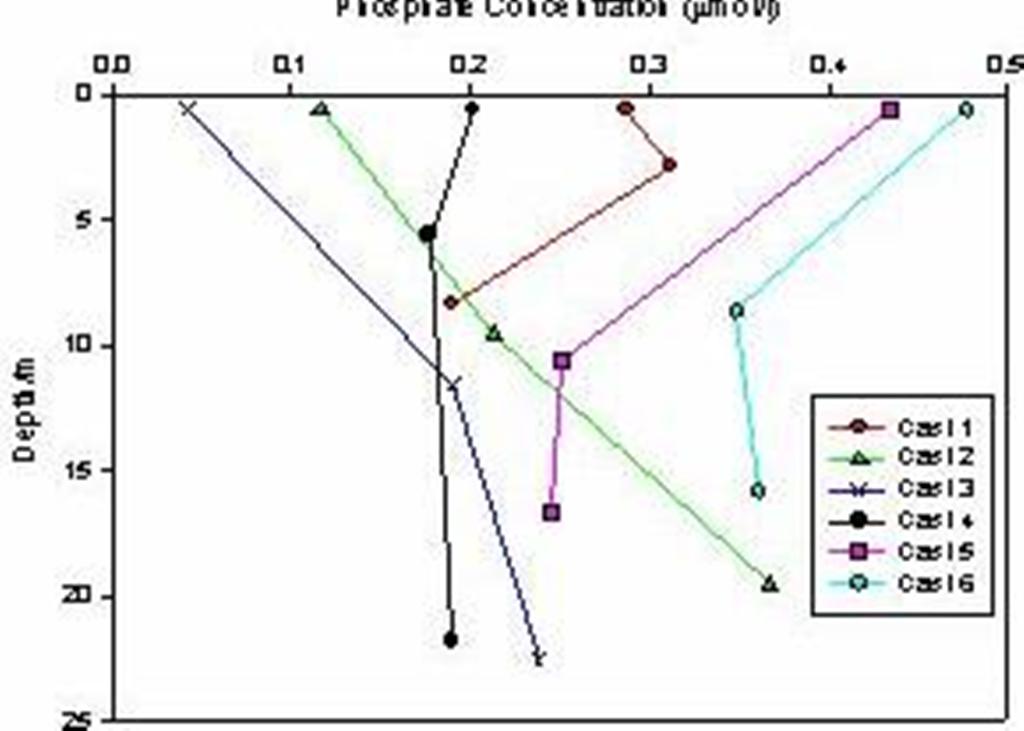
Figure 21. Phosphate plotted with depth at stations 1 to 6.
As per figure X the Phosphate data are above the detection limit. Phosphate concentrations do not increase along the estuary. This is as expected as there is non-conservative mixing, with both addition and removal. Methods of addition are from sources such as sewage, detergents, fish farms, and run off. The phosphate in the Fal estuary is heavily impacted by sewage inputs. The position of these can be seen in figure 23. Removal can occur by biological means or suspended solids. As the concentrations of phosphate are low, even small amounts of removal or addition can impact the concentrations. Station 3 showed the lowest concentration of phosphates (Figure 21). Samples from the depth and the thermocline were relatively homogeneous between 0.2 and 0.4 µmol/l. At the surface low values were seen at the mouth of the river, in samples 2, 3 and 4, which could be due to dilution or biological removal. Sample 1 showed intermediate values which could be due to addition by anthropogenic discharges. Samples 5 and 6 showed the highest values at the surface which is expected as these are at the top end of the estuary where there is increased addition from the rivers.
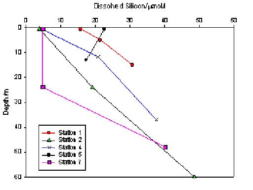
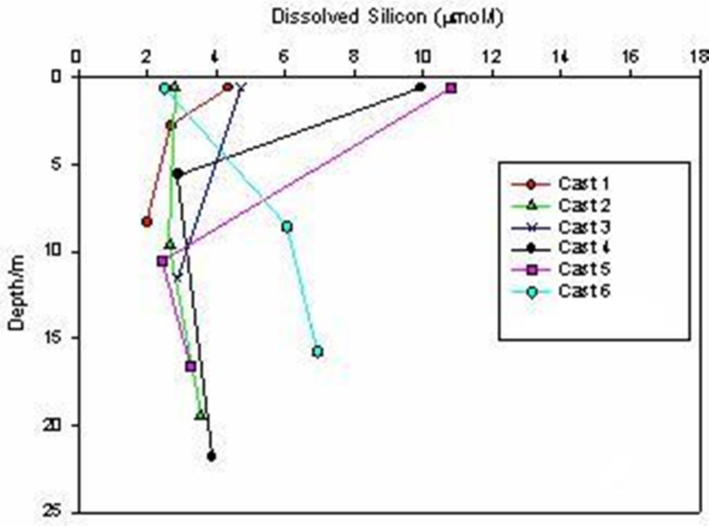
Figure 22. Dissolved Silicon plotted with depth at stations 1 to 6.
As per figure 22 the Silicon samples are above the detection limit. Silicon shows a non-conservative relationship at high salinities. As samples were not collected from low and intermediate salinities it is difficult to determine whether Silicon is conservative or if there are additions or removals. Additions of silicon are due to weathering and removal is due to biological processes by Diatoms. The samples at depth were relatively homogeneous except for sample 3. This sample has been noted as an outliner. At the surface the lowest values were seen in sample 6 at the head of the estuary. This may be due to removal by diatoms. Surface values in samples 1, 2 and 3 are in line with the amounts at depth. Samples 4 and 5 have high surface values which may be due to the increased rainfall and weathering.
Figure 23. Larger discharges in to the Fal Estuary (Langston et al., 2003)
Table 2 shows the detection limits for chemicals analysed during the fieldcourse Discussion The Fal Estuary and neighbouring creeks were shown to be highly eutrophic. This was mostly due to the high amounts of rainfall in the days preceeding the field course and hence a high river runoff. Estuarine mixing diagrams from the estuary for nitrate and silicate indicate that the nutrients are behaving conservatively with regards to salinity. There is no indication that addition or removal is occurring, however as nutrient samples were only collected at a limited range of salinities this is not conclusive. Phosphate, on the other hand, showed considerable amounts of non-conservative addition and removal. The addition is probably due to external input (for example, sewage). The removal of phosphate is probably due to biological removal and suspended sediment processes. The nutrient eutrophication stimulated high phytoplankton concentrations. Phytoplankton concentrations can be directly correlated to the chlorophyll concentrations as chlorophyll is found within phytoplankton cells. The highest phytoplankton concentrations were found at the mouth of the Fal estuary, with numbers decreasing to the mid estuary and then increasing again in the upper estuary. The chlorophyll and hence phytoplankton concentrations are at maximum levels around the thermocline vertically. Concentrations decrease below the thermocline due to a lack of light (shallow euphotic zone)and above the thermocline due to a lack of macronutrients. Clearly shown on the ADCP, was the predation of phytoplankton by zooplankton. This was seen as a layer of zooplankton on either side of the chlorophyll maximum (phytoplankton concentration maximum).
Temperature and salinity profiles in the estuary and its tributaries indicate stable stratification throughout the estuary. This was clearly identified by a deepening thermocline moving toward the estuary mouth. There should be further studies concentrated on observing nutrient distributions over many salinities and covering multiple tidal states to provide a more accurate view of the Fal estuary. It can be noted that the physical chemical and biological structure of the fal estuary was directly influenced by the input of fresh water by the river fal and neighbouring tribrutaries
|
|||||||||||||||||||||||||||||||||||||||||||||||||||||||||||||||||||||||||||||||||||||||||
|
Introduction On the 4th of July 2007, a geophysical survey was carried out at a selected area at the mouth of the Helford estuary, using the M/V Grey Bear landing craft. The aim was to analyse the sediments and the biology of the benthic habitat. Conditions were blustery with winds of up to 27 knots and averaging 25 knots through the day. A side scan sonar survey was completed over four transects, each measuring 2.33km. The survey began at 09:40GMT and was completed at 11:35GMT. The side scan sonar traces were then reviewed for possible sites to take grabs of the underlying sediment. The grab samples were used to ground truth side scan records and help differentiate between the observed seabed packages. The samples were taken from areas where we saw a large contrast in backscatter which indicated different sediment types. Grabs were taken in areas of soft sediment using a Van Veen Grab. Five grabs were taken, four close to the mouth of the estuary and one from a location further offshore. The samples were taken between 12:12GMT and 13:23GMT. From these grabs the sediment type and biological composition were analysed. Equipment
Results Figure 24 shows the completed track and contrasting sediments within a 1.8km2 area at the Helford estuary.
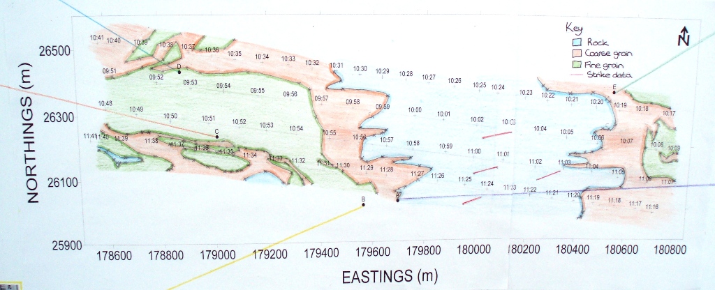
The red shaded regions show areas of coarse grain sediment whereas the green shaded regions represent finer grained sediment. The blue shaded region to the west of the study site indicates bed rock. The letters A-D represent the grab sites taken after the side-scan sonar. The data from the grab samples will be discussed later.
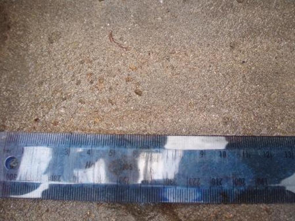
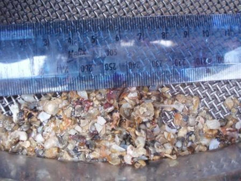
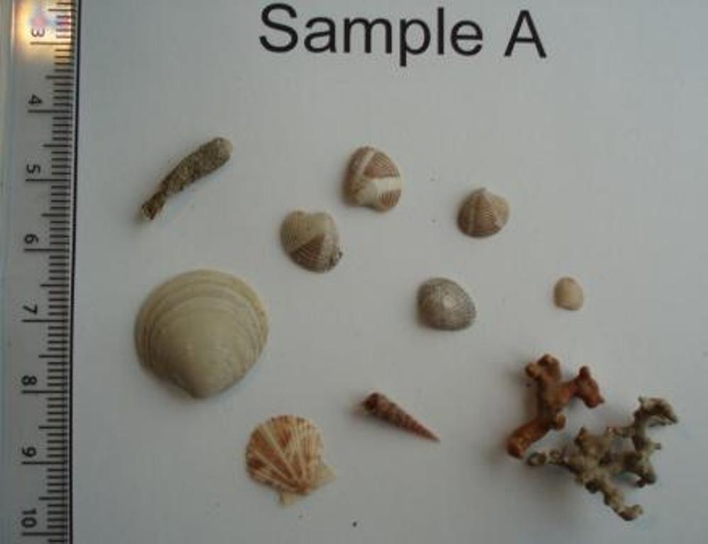
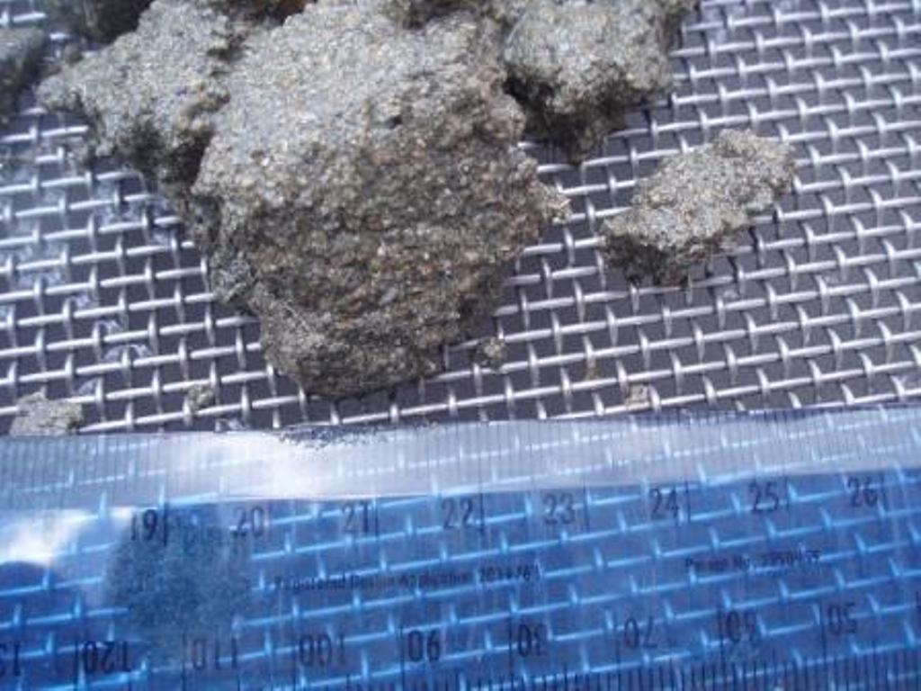
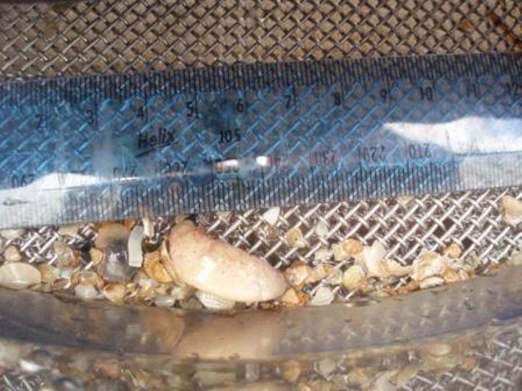
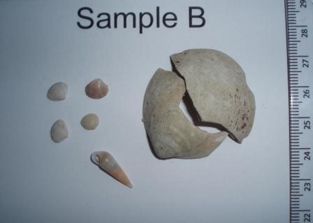
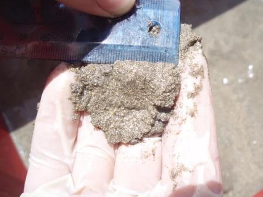
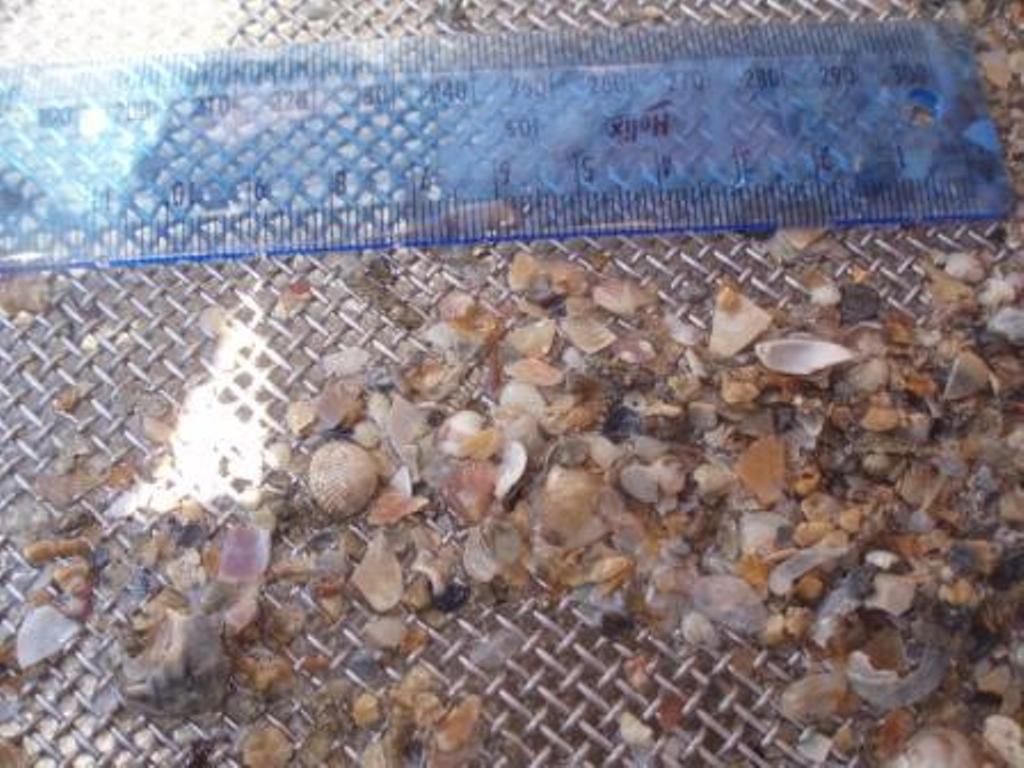
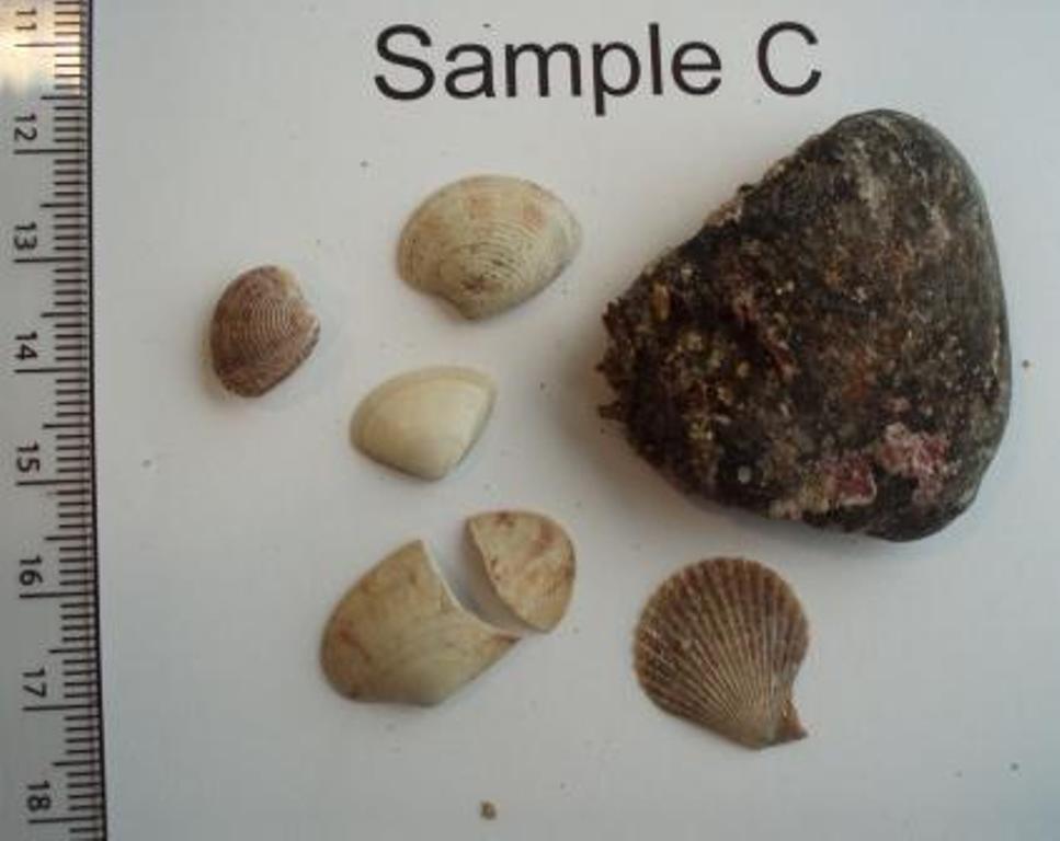
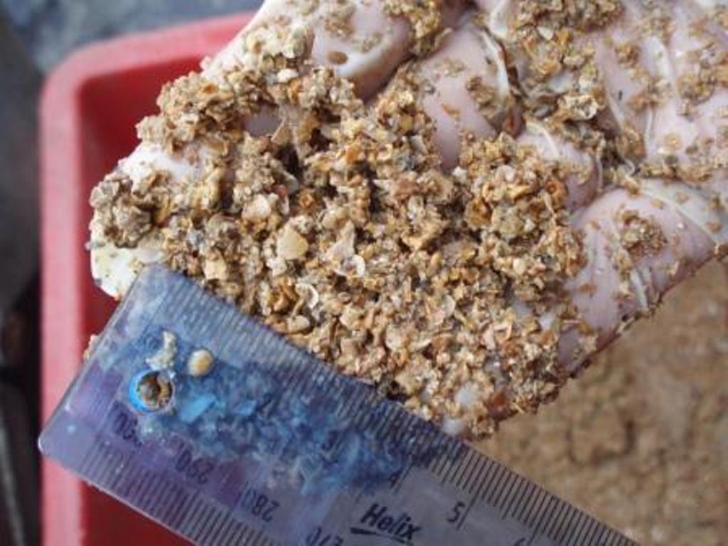
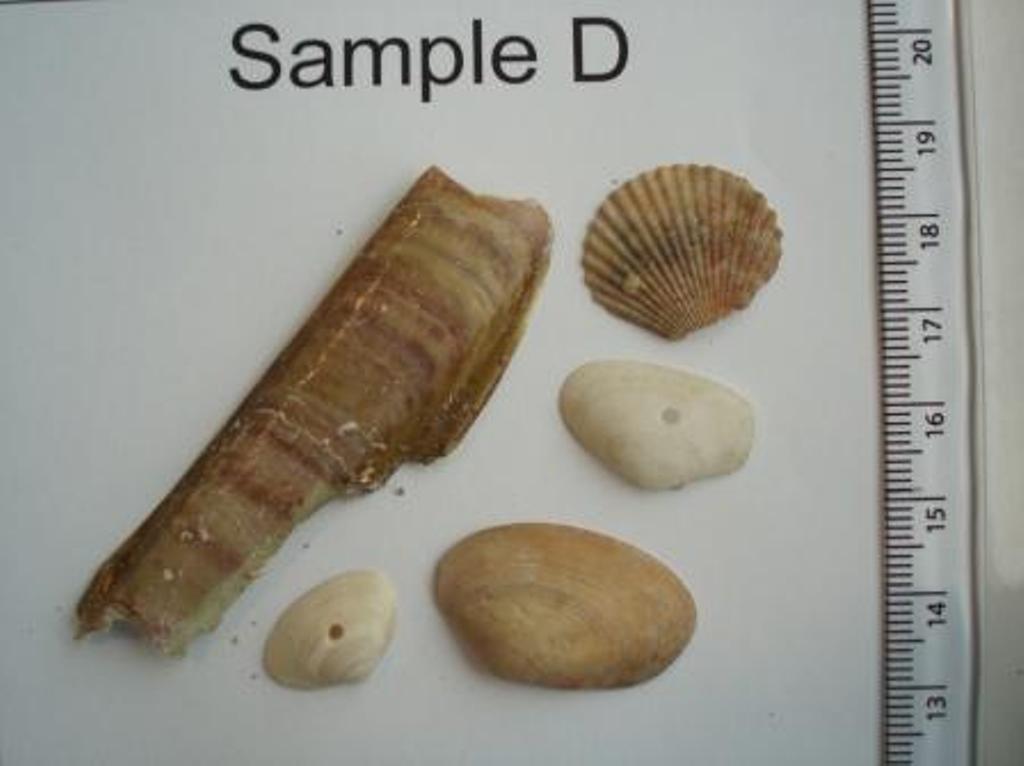
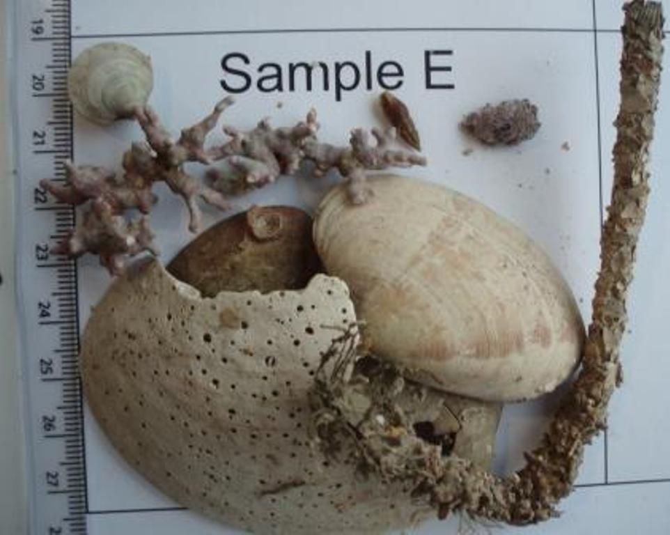
Figure 24. Completed track showing contrasting sediments within a 1.8km2 area at the Helford estuary. The Falmouth regional strike orientation is north-easterly. (Leveridge et al., 1990) According to the side scan data collected at the mouth of the Helford estuary the strike in this area is also in this direction as can be seen from the track plot. the red lines on the plot indicate the direction of the strike that was observed on the side scan trace. Sample information The sediment of Samples A, B & C were uniform and included fine sediment and muds. Sample D was made up of coarser sediment and Sample E included a large proportion of dead Maerl. Numbers of live organisms were low in all samples and all samples included bivalve shells. The following tables and figures give a summary of the conditions at each site and the sediment and biological properties (table 3-7 and figures 25-29)
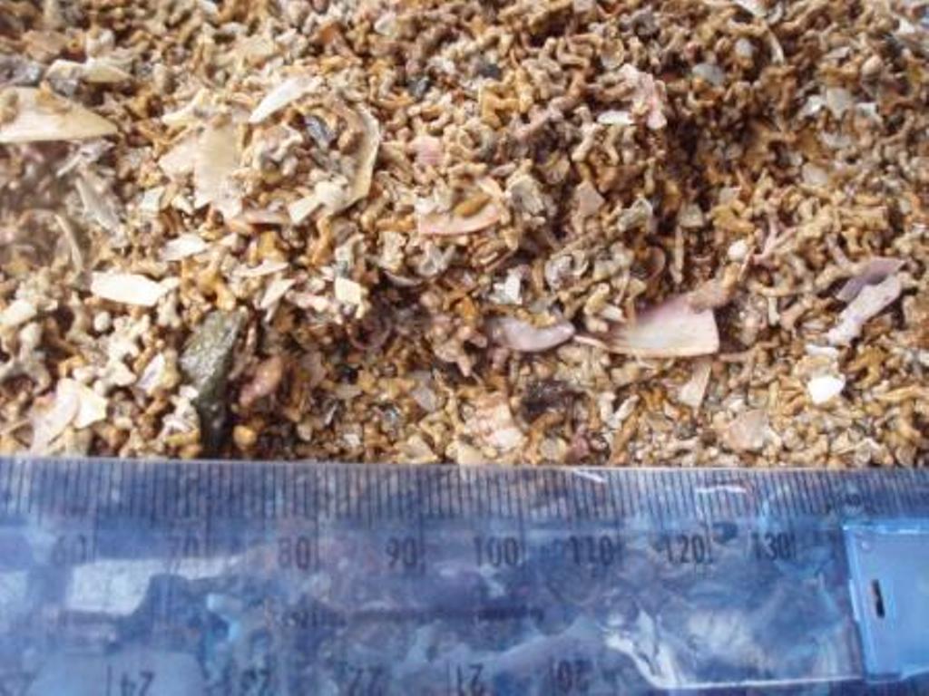
Discussion The grabs obtained showed little difference between locations. The main constitution was of fine bioclastic sand, mud and broken shells. The grain size of the sand present within the last two grabs was of a coarser nature.
The living macrobiota present within all grab sites was limited, although a number of worms, bivalves, a small harbour crab and an Echinoderm was identified. There was an abundance of broken shells mixed into the sand, mainly composed of bivalve and small king scallop shells.
The area was recently deemed as a Special Area of Conservation (SAC) (www.jncc.gov.uk) and the area is still in the very early stages of recovery from past mining activites and which still continues to influence the region via mine discharges and the resuspension of metals from sediments.
A particular reason why this district was given the title of SAC is due to the extensive Maerl beds found within the lower Fal, however, if any live Maerl was present in the sample grabs, these were only of diminutive frequencies compared to dead Maerl. However, even small numbers of live Maerl have the potential, if undisturbed over large periods of time, to fully re-establish a successful and extensive population.
Live Maerl was found in the first and last grab samples (positions 50˚05’606, 5˚04’890 ; 50˚05’807, 5˚04’206 respectively), in comparison to dead Maerl. The last grab sample was largely composed of dead Maerl.
Regarding the underlying topography of the area surveyed, there are numerous geological and geographical features identified via the sidescan sonar. As shown on the trackplot, there is clearly an indication of a long stretch of rocky terrain, surrounded either-side by beds of fine and coarse sands with patches of dead Maerl beds. The rocky stretch frequently featured high structures, some measuring more than 2 metres high, and is possibly a remnant of the tectonic plate activity prevalent in much of the surrounding coastline.
|
|||||||||||||||||||||||||||||||||||||||||||||||||||||||||||||||||||||||||||||||||||||||||
|
The aim of the practical was to analyse the physical properties offshore of Falmouth estuary as well as taking water samples to observe the chemical and biological structures within the water column both on the well mixed and stratified side of a frontal system.
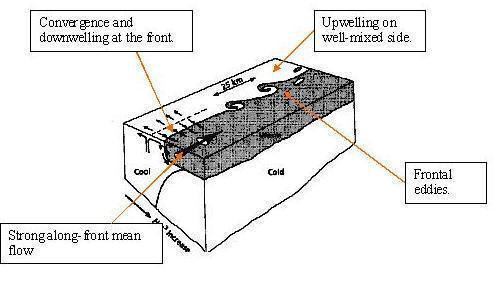
Table 8 showing conditions during offshore study Equipment used A hull mounted Acoustic Doppler Current Profiler (ADCP) was used to analyse the physical properties within the offshore water column. The group used this device to seek out frontal systems and monitor water density and velocity. The ADCP was used for a total of 5 transects. A 5 Niskin bottle rosette system was deployed via an A frame to provide sea water samples which were later analysed for chemical studies (Oxygen saturation, Chlorophyll, Silicate, Nitrate and Phosphate concentrations). The rosette system was also used as frame for a CTD apparatus (Conductivity / Temperature / Depth). Conditions allowed for a total of 8 CTD drops. A plankton net with mesh size of 200 µm and a diameter of 59cm was used to conduct vertical hauls from depth to the apparent thermocline and from the thermocline to surface, to study the vertical distribution of zooplankton in the water column. Plastic bottles were used to store silicate and chlorophyll samples as well as zooplankton samples for the study of community structure. Glass bottles were used to store Phosphate and Nitrate samples. Frontal Systems Fronts are regions of larger than average horizontal gradients of water properties, these include temperature, salinity, density, turbidity, and colour. The formation and location of frontal systems depends on 2 principal factors during the summer seasons: 1) Tidal mixing and tidal stream velocity 2) Depth of the water column (Mann and Lazier,1996)
The position of the frontal system was in previous studies discovered to run parallel to the coastline at a range of roughly 8 nautical miles offshore. However on finding the front it was discovered that it had been displaced so that the system directly offshore from the estuary was at 6.5 nautical miles, to the East of the estuary however the front was observed to move much closer inshore to within 1.5 nautical miles of the shoreline 9.5 nautical miles up the coast from the Fal estuary.
Our hypothesis for this finding is that the riverine output from the Fal and Helford estuary in this period of high rainfall forced the area of well mixed water further from the coast in the vicinity of the estuary mouths. In the area to the east of the estuary where the fresh water output is only through ground water runoff, the front impinges far closer to the shoreline than was predicted. This effect would be especially noticeable during the ebb of the tide where the water would be forced out at a greater rate. a transect across the mouth of the Fal estuary was taken 6 hours before high water with a ADCP. The rate of discharge from the estuary at this time was measured as 414m3/s, this combined with the discharge from the Helford estuary may cause the area of well mixed water inshore to be forced further into the English channel. The flooding tide could also be responsible for forcing the front closer to the shore during the flood tide which coincided with the time when we sampled the area to the east of the Fal.
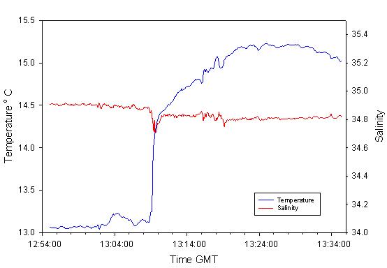
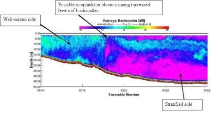
Figure 32.5 shows one of the inshore transects taken from the R/V Callista. The inshore portion is towards the left hand side of the figure with the track moving in a south westerly direction as the diagram moves right. At ensemble point 5168 a clear boundary can be seen with high degrees of mixing on the LHS and high stratification on the RHS. The boundary is marked with an area of extremely high backscatter. A likely cause for this distinct line would be the re-introduction of nutrients from the well mixed zone into the nutrient depleted upper waters of the highly stratified side. This would cause a strong bloom in phytoplankton production which would be closely followed by an increase in the zooplankton population.
Fig 32.5 ADCP image of the Front.
Chlorophyll Stations
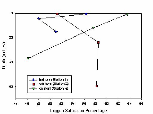
Nutrients The following will discuss the nutrient samples with depth from the offshore environment. Phosphate, Silicon and Nitrate are all within the detection limits for the analysis. Samples were taken from depth, the thermocline and the surface. The first sample was taken at Black Rock within the estuary. Sample 2 was taken after crossing the front. This sample was therefore in the offshore stratified region with a temperature difference of 2.5°C from the surface to depth. This site had the highest surface temperature of the sampled sites. Sample 4 was taken within the front. Sample 6 shows the inshore side of the front that displayed less of a thermocline with a temperature difference of 0.5°C from the surface to depth. Only surface and depth samples were taken due to CTD failing to fire. Station 7 was taken within a front and was the furthest sample obtained offshore. This site was also stratified with a temperature difference of 2.5°C.
Oxygen
supply, produce further oxygen via photosynthesis, however, the extent to which this occurs is light dependant, and as a result decreases with depth. Below the thermocline there is less mixing, as a result there is a smaller population of phytoplankton using up the nutrient supply and hence there are fewer individuals respiring. Consequently the oxygen supply in this region of the water column is not used to the same extent. Information under the heading ‘Further Studies’ will explain how the data acquired at the other sampled stations could be used and improved to arrive at a more conclusive interpretation of how oxygen levels behave in the offshore water column. Fig ***shows how oxygen saturation concentrations change with depth in the offshore water column at various stations sampled, each with a given reference to their relative position before, on, and after the frontal system.
Phytoplankton
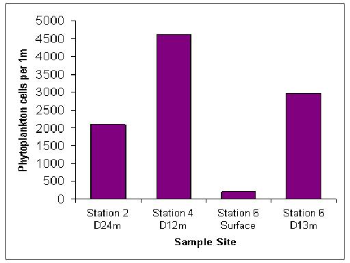
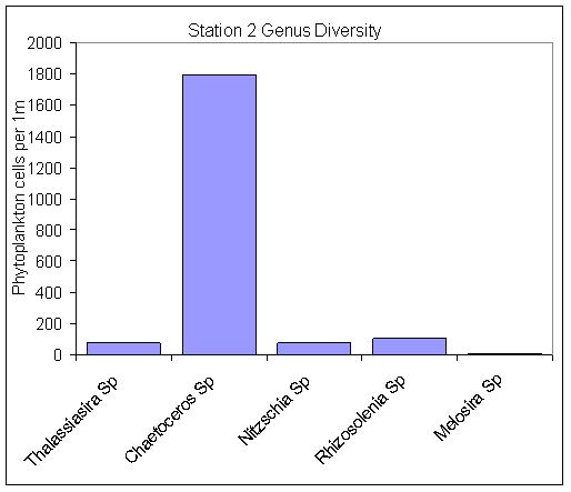
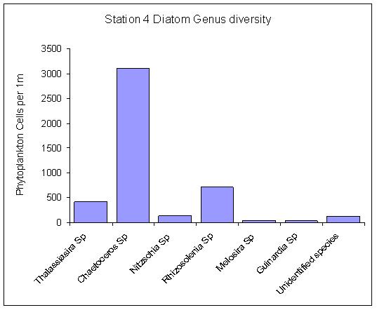
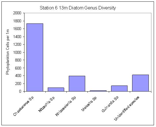
Highest levels of Phytoplankton were recorded at Station 4 at 4m depth with 4460 Phytoplankton per 1m, only Station 6 Surface sample collected figures less than 1000 Phytoplankton. The dominant form of phytoplankton found in all samples were diatoms, particularly species of Chaetoceros. Other Genus found in high numbers include; Thalassiasira, Rhizosolenia and Nitzschia. Species of Dinoflagellates found included Ceiatium fusus and Alexandrium. A few Cilliates were identified as Mesodinium rubruui and Haptophytes were identified as Phaeocytis globosa at two stations in low numbers. (Fig .39.)
Fig .39. Graphs showing the total number of phytoplankton cells per 1ml from four samples collected at varying points along the front. Genus diversity was greatest at Station 4 D12m with 6 genuses being identified with 125 phytoplankton species per 1m remaining unidentified. The Station 6 surface sample showed the least diversity with significantly less species and total numbers of phytoplankton; only 2 genus identified and of which 92% (195 phytoplankton per m) were Chaetoceros. Dinoflagellates and Ciliates showed less diversity and fewer numbers were recorded, Alexandrium and Ceiatium fusus being the most abundant recorded. One species of Haptophytes was identified as Phaeocytis globosa and was present at station 2 and the 13m sample from station 6. Fig .40. pictures some of the groups of phytoplankton found
Zooplankton
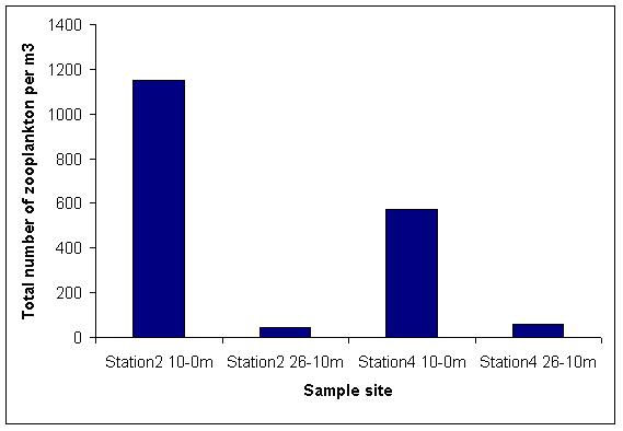
Zooplankton samples were collected from two vertical transects at two stations, determined by their position in relation to the front. Station 2 was located offshore from the front whereas station 4 was within the front. CTD data from these two stations indicates a stratified water column offshore of the front and a well-mixed water column within the front. ADCP profiles agree with the CTD data, with a high area of backscatter indicating a zooplankton sandwich between 20-25m at station 2, this suggests a stratified water column and large chlorophyll maxima region. This is confirmed with flourometer readings, which show a chlorophyll maxima from around 15-25m. Phytoplankton samples collected at 24m showed concentrations of 2085 per ml, which again correlates well with the ADCP profile. However the samples suggest low zooplankton abundance (46 individuals per m3) at this depth compared to a very high abundance (1148 individuals per m3) in the top 10m’s (Fig .41.). CTD data for station 2 shows a thermocline at around 11m, which correlates more to the zooplankton sample data. Zooplankton would be expected to be in high abundance above the thermocline where the phytoplankton would be found.
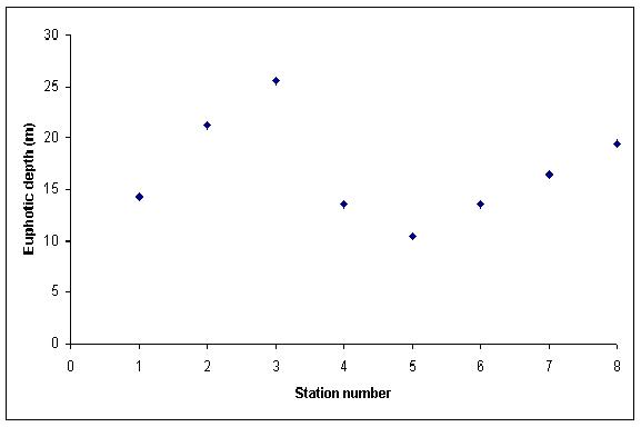
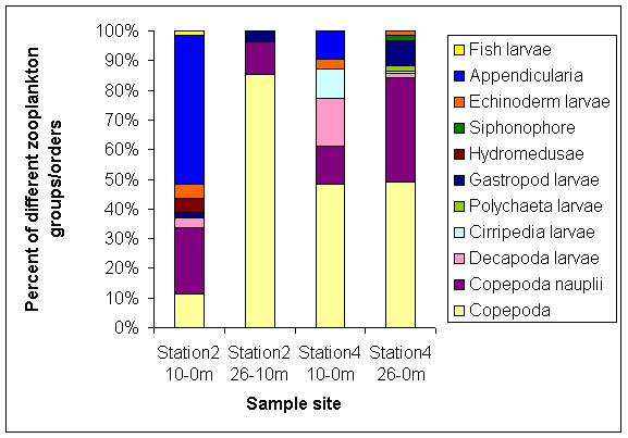
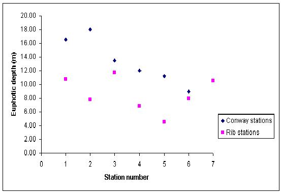
Station 4 also shows a larger number of zooplankton per m3 in the upper 10m (574 individuals per m3) of the water column compared to 26-10m (60 individuals per m3) (Fig .41.). The ADCP profile for this station agrees with the CTD that the water column is well mixed showing no indication of a zooplankton sandwich and therefore a thermocline. There is a very high amount of backscatter within the top 5m of the water column, most likely from a high abundance of zooplankton. The euphotic depth (taken from secchi depths, was recorded as 13.5m at station 4 compared to 21.3m at station 2 (Fig .42.). The mixing of the water column is likely to bring about higher turbidity and therefore a reduction in the water clarity, this would limit the depth of available light and could therefore affect the depth at which phytoplankton and hence zooplankton would be found. Flourometer data agrees with the secchi disk measurements showing a chlorophyll maxima at around 13m, due to the lack of stratification the readings from the flourometer show a gradual decrease below this point. Phytoplankton samples collected at this station from 12m depth showed concentrations of 4620 per ml agreeing with the flourometer readings. The abundance of phytoplankton at this depth could explain the higher numbers of zooplankton within the top 10m of the water column. Station 4 and at depth at station 2, the dominant zooplankton were identified as Copepoda (around 50% and 85% respectively), whereas within the top 10m of station 2 the dominant zooplankton were Appendicularia (50%), with a relatively low percent of copepods (11.29%). (Fig .43.) The variance between the two samples at station 6 can partly be explained by observing the fluorometer readings taken at the same site. This suggests that Chlorophyll was at its minimum at the surface and its maximum at about 8 meters the sample being taken at 13m would therefore be expected to contain more phytoplankton than at the surface but less than a sample taken nearer to the chlorophyll maximum. The waters were also well mixed and inshore of the front which would mean conditions would be less favorable than a more stratified location close the front which is where station 4 was sampled, there the chlorophyll maximum was at 18m. Frontal conditions would be rich in nutrients and well mixed however, near the front the nutrients will be able to mix into more stratified layers replenishing the euphotic zone allowing phytoplankton to utilize the maximum amount of nutrients without depleting them completely. Discussion The data collected on the Callista showed that the water column became more thermally stratified and hence the water column was very stable further offshore. We see a typical plankton community develop in the increasingly stable water column. Both nutrient and internal water mixing contribute to the distribution of phytoplankton in the water column. The station found within the Fal estuary showed a water column that was well mixed due to stronger tidal mixing, preventing the formation of a strong seasonal or diurnal thermocline. Such strong mixing was shown on the ADCP profile from this station as high water velocities throughout the water column, with internal velocities decaying at the offshore stations. During the R/V Callista investigation offshore, a sudden rise in temperature while traveling (from inshore to offshore) indicated the location of a front. The inshore side of the front was well mixed with high nutrient surface waters but low chlorophyll surface waters. This was due to high vertical mixing which causes the phytoplankton to be moved downwards in the water column to below the euphotic zone, an area where there is insufficient light for photosynthesis to occur. On the offshore side of the front, the water column was found to be more stratified because of the depth of the water column and the lack of internal and tidal mixing. The surface water on the offshore side of the front also had a small phytoplankton population which may partly be due to the lack of surface nutrients from the utilisation by a previous phytoplankton bloom. As a result, phytoplankton populations reached a maximum deeper in the water column due to a deeper euphotic zone and seasonal thermocline. Growth here was therefore nutrient limited. The chlorophyll maximum occurred at a similar depth to that of the peak phytoplankton concentration. In these cases, the phytoplankton are being held in the upper layer of the water column due to the stable stratification that has developed, enabling them to photosynthesize effectively. The zooplankton tows conducted offshore were dominated by both larvaceans and copepod nauplii
|
|||||||||||||||||||||||||||||||||||||||||||||||||||||||||||||||||||||||||||||||||||||||||
|
From the 3rd to 14th July 2007, the Fal Estuary and the surrounding area was systematically surveyed to provide a scientific view of the physical, chemical, biological and geophysical properties of the rivers, estuary and offshore. This was done using a large range of equipment and vessels over the three days of on water research, followed by consecutive days of labs work and data analysis. Nutrients were found to behave in conservative and non conservative ways. With the nitrates being the only conservative nutrients and additional phosphate and silicate being added during the waters time in the estuary. In the offshore areas nutrient profiles behaved as expected with depleted surface concentrations and higher deep water concentrations. The maximum surface concentrations were found on the well mixed sides of the fronts. Phytoplankton populations were found to initially decrease with salinity with relatively high concentrations found at the head of the estuary. Towards the mouth populations were found to increase again. The highest concentrations of phytoplankton were found around the frontal regions where nutrient rich well mixed cold waters met warm nutrient poor stratified water. Zooplankton populations were found to vary in both density and diversity with position in the estuary. Populations found in the head of the estuary were found to be dominated by Copepoda nauplii with populations found in the mouth being dominated by Copepoda. Stratification in the estuary was dominated by the input of fresh water from the surrounding creeks and rivers. Outside of the estuary this stratification was broken down by strong tidal streams and coastal mixing process. Strong thermoclines were found offshore with gradients of up to 3°C. This change from highly stratified waters to well mixed created distinct fronts parallel to the shore line. While investigating these fronts on the R/V Callista it was found that there position was strongly influenced by tidal and fresh water movements. Frontal systems around the mouth of the Fal were forced offshore by the freshwater output of the river with the front further along the coast being forced inland by the incoming tide. The Fal estuary and the surrounding coastal areas are part of a complex system of physical, chemical and biological factors. This investigation has only looked at a very narrow part of the overall system. For a greater understanding of the whole situation further studies are required of many different areas. Some initial ideas are shown in he next section.
|
|||||||||||||||||||||||||||||||||||||||||||||||||||||||||||||||||||||||||||||||||||||||||
|
Due to time constraints, parts of the Fal Estuary could be more comprehensively sampled in future studies, to gain a better overall account of the processes and influences of the region. More grab samples can be undertaken to determine the nature of the underlying sediment, as these often contribute and are representative of the overlying water column. A sidescan survey should also be carried out to provide locations on the best whereabouts of potential grab sites. This will also extend the data series that was obtained on the Grey Bear, allowing a proper survey of the estuary. Laboratory simulation and computer modeling of different mixing processes can carried out alongside data collected on the research vessels to look for patterns of correlation. More extensive sampling of the phytoplankton communities could reveal an insight on what role they play within the estuarine environment. The research undertaken by the Grey Bear could be improved by adding more sidescan transects to either side of the area plotted at the mouth of the Helford Estuary. This would further increase the area of observation and discern whether the patterns already distinguished are isolated or continuous. Furthermore, a set of higher-frequency sidescans could be taken over areas of interest alongside the usage of more grabs. This would aid in the classification of underlying sediments and could be used subsequently as a key to locate Mearl beds for survey by interested parties. Similarly, the use of divers and remotely operated vehicles could be used to confirm and compliment this information. If possible a 24 hour (or longer) stationary time series should be carried out to determine the normal daily water fluctuation parameters of the estuary. This would give an indication of acceptable fluctuation ranges of water bodies within the estuary. A similar stationary time series should be undertaken offshore as many of the chemical results will change dramatically within the space of 24 hours. This could give an index of the range in which parameters can change when travelling from one station to the next. Oxygen saturation levels, for example, can vary from a state of supersaturation in the day to heavily depleted levels at night. With this knowledge, the interpretation of graphs could be further understood.
|
|||||||||||||||||||||||||||||||||||||||||||||||||||||||||||||||||||||||||||||||||||||||||
|
Langston W., Chesman B., Burr G., Hawkins S., Readman J. & Worsfold P. 2003. Characterisation of European marine sites. The Fal and Helford, 2003. Marine Biological Association Mann K., Lazier J. 1996. Dynamics of marine ecosystems.Blackwellscience Leveridge B., Holder M., Goode., 1990.geology of the country around Falmouth.Memoir of the British Geological Survey. Sheet 352 Google Earth Fish J. & Carr H. (1990). Soud Underwater Images. Guide to the Generation and Interpretation of Side Scan Sonar Data. Lower Cape Publishing Tait R. & Dipper F. (1998). Elements of Marine Ecology. Butterworth-Heinemann http://www.generaloffshore.co.uk/greybear.html http://www.soes.soton.ac.uk/resources/boats/ www.dnr.state.md.uswww.soes.soton.ac.uk/resources/boats www.generaloffshore.co.uk/greybear
|
|||||||||||||||||||||||||||||||||||||||||||||||||||||||||||||||||||||||||||||||||||||||||
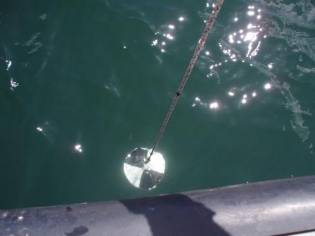 The
rate of decrease of illumination with depth is known as the
extinction coefficient (k). A Secchi disc provides a simple method
to determine a rough measurement of the extinction coefficient. The
Secchi disc is either white or alternating black and white
quarters. The disc is lowered in to the water and when it
disappears from sight the depth (d) is noted. The extinction
coefficient can then be determined from the relationship k=1.45/d (Tait
& Dipper, 1998). The Euphotic Depth can also be determined by
multiplying the Secchi disc depth by three.
The
rate of decrease of illumination with depth is known as the
extinction coefficient (k). A Secchi disc provides a simple method
to determine a rough measurement of the extinction coefficient. The
Secchi disc is either white or alternating black and white
quarters. The disc is lowered in to the water and when it
disappears from sight the depth (d) is noted. The extinction
coefficient can then be determined from the relationship k=1.45/d (Tait
& Dipper, 1998). The Euphotic Depth can also be determined by
multiplying the Secchi disc depth by three. 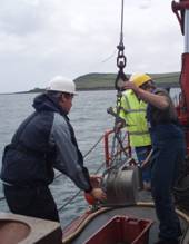
 Side
scan Sonar
Side
scan Sonar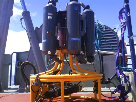 A
CTD profiler is used to measure conductivity (salinity), temperature
and depth. A thermistor, a platinum thermometer or a combination of
both, are used to measure temperature. Pressure and therefore depth
are measured using either a strain gauge pressure monitor or a
quartz crystal-based digital pressure gauge. CTD profilers are
favourable due to their accuracy. Salinity measurements are accurate
to 0.005, temperature measurements to 0.005
A
CTD profiler is used to measure conductivity (salinity), temperature
and depth. A thermistor, a platinum thermometer or a combination of
both, are used to measure temperature. Pressure and therefore depth
are measured using either a strain gauge pressure monitor or a
quartz crystal-based digital pressure gauge. CTD profilers are
favourable due to their accuracy. Salinity measurements are accurate
to 0.005, temperature measurements to 0.005
 A
A