![]()
GROUP 3

NAVIGATION

Dave Watkins, Thomas Slater, Andrew Eggett, Abby Bull, Dominic
Harris, Adam Wilkinson, Nathan Robinson,
Frances O'Hara, Jennifer Wright, Xavier Laurent and Westley Heydeck
NAVIGATION
The Fal Estuary
The Fal Estuary is located on Cornwall’s south coast and stretches 17km between the head of the Tresillian River and the western end of the English Channel. It is supplied from 6 main tributaries as shown in Figure 1. The main body running through the centre is known as Carrick Roads, and forms the deepest part of the channel.
|
|
|
Figure 1. The Fal Estuary and associated creeks. |
The Fal Estuary is a Ria (drowned river valley) with a mean coastal water temperature of 16˚C in the summer and 9˚C in the winter. The mean tidal range is about 5m and tidal currents are usually below 2 knots. Prevailing winds are generally from the South West. The Carnmellis granite and surrounding metamorphic rocks to the West represent the underlying geology of the estuary, and these are reflected in the sediments and overlying water column
Maerl is a calcareous algae found on the seafloor at certain locations within the estuary, and its existence, along with the Zostera beds, has led to the Fal being named as a Candidate Special Area of Conservation.
The Fal Estuary is affected by many pollution processes. Creeks draining into the estuary all contain varying quantities of heavy metals within their sediments. Industrial activity impacts upon the contaminants entering the area, the most notable activity throughout the ages being mining. During the nineteenth century the catchment for the Fal Estuary included regions with copper, tin and arsenic mining. Copper mining ended with the turn of the century, but tin mining continues to this day, and run-off into the estuary still causes contamination.
The Fal Estuary is an important harbour, with the availability of moorings for recreational vessels as well as docking and repairs services. Consequently, the tributyltin compounds used as antifouling paints on ships also contaminate the area. This compound is reported to lead to a phenomenon known as imposex, which is the effect of female organisms developing male characteristics (Smith, 1971), and has been observed in dogwhelks in the Fal Estuary.
The effect of the pollution in
the area has been surveyed and organism distribution has been observed
to have been altered as a result. Restronguet Creek has the highest
contamination levels within the estuary, and the Fal is the most metal
polluted system in the UK Under certain conditions metals are toxic to
organisms, but despite the high heavy metal content creating a hostile
environment certain organisms are adapted to live in these conditions.
For example, copper levels within the Fal Estuary are reported to have
reached dry weight levels of up to 3000 µg g-1, and oysters
are dyed green from the contamination. The intensity of the green
colouration of the oysters reflects the concentration of the copper.
Below are the results of an intensive survey of the Falmouth region.
Estuaries - Date: 3/7/07 - Day 1
NAVIGATION
Aims:
To assess the nutrient concentration levels within the estuary and establish the phytoplankton and zooplankton communities. Also to analyse the physical properties, such as temperature, salinity and flow velocity, of the Falmouth Estuary.
Objectives:
-
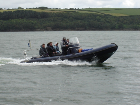
RIB – To sample the water at various selected stations throughout the upper reaches of the estuary.
-
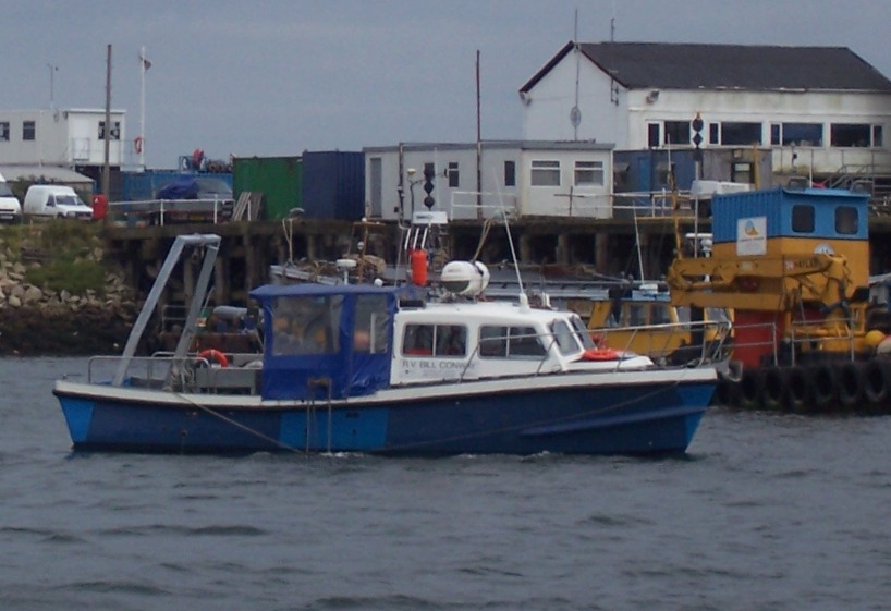
Bill Conway – To sample the middle and lower reaches of the estuary at a sufficient number of stations, each determined by a measured decrease in salinity of 1.5.
-
To assess the non-conservative or conservative mixing behaviour of nitrate, phosphate and silicate up the estuary.
-
To establish some level of understanding of the mixing and flow of the estuary via longitudinal and transverse transect sampling.
-
To sample quantitatively and qualitatively the various phytoplankton and zooplankton communities found at different levels of the estuary and compare these to nutrient levels, dissolved oxygen concentration, turbidity and the light attenuation data.
Sampling strategy:
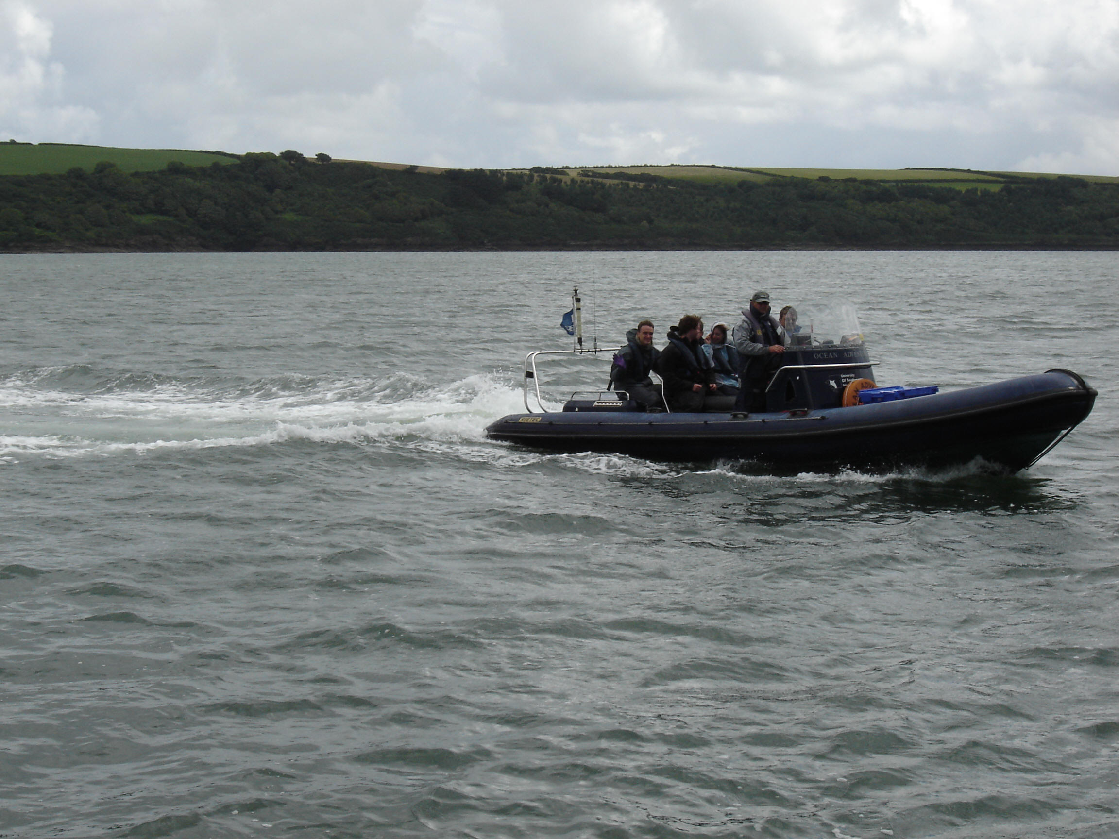
Two slightly different sampling strategies were used in order to collect
the data required on each boat. Sampling onboard the smaller RIB
involved vertical profiling of temperature, salinity, chlorophyll and
transmission using a YSI probe, Niskin bottles were deployed and closed at
specific depths to collect samples for nitrate, phosphate, silicate and
dissolved oxygen. These water samples were also filtered onboard to
remove and measure chlorophyll and a 200μm net was deployed for 10 minutes
into the river and held in place by the current to measure zooplankton.
Sampling was carried out at 6 specific mooring stations (Figure 2.1.1) in the upper
estuary at which the RIB could dock whilst sampling.
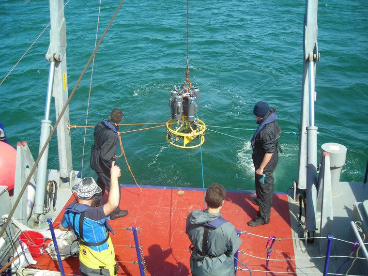
 Sampling onboard
the larger Bill Conway consisted of vertical CTD profiles (Figure 2.1.2)
measuring a similar range of features as the YSI. Attached was a rosette
of Niskin bottles for analysis of nutrients, chlorophyll and dissolved
oxygen. Light attenuation was measured using a Secchi Disk, a zooplankton trawl was also deployed. Sampling was
carried out at locations determined by changes of 1.5 salinity throughout the
lower and middle reaches of the estuary.
Sampling onboard
the larger Bill Conway consisted of vertical CTD profiles (Figure 2.1.2)
measuring a similar range of features as the YSI. Attached was a rosette
of Niskin bottles for analysis of nutrients, chlorophyll and dissolved
oxygen. Light attenuation was measured using a Secchi Disk, a zooplankton trawl was also deployed. Sampling was
carried out at locations determined by changes of 1.5 salinity throughout the
lower and middle reaches of the estuary.
Tides and Weather (3/7/07):
|
|
Time (GMT) |
Depth (m) |
Weather: |
|
1st Low Water |
0111 |
1.1 |
At the mouth of the estuary: 6/8 cloud cover, mainly cumulous and stratocumulus clouds with a wind speed of 6 knots. The wind direction was south westerly. |
|
1st High Water |
0702 |
4.9 |
|
|
2nd Low Water |
1328 |
1.2 |
|
|
2nd High Water |
1911 |
5.2 |
Equipment:
|
Middle & Lower Estuary: Bill Conway |
| ACDP plus ADCP software - Winriver |
| CTD (F7a) and frame (F7d) inc. Fluorimeter (F9a), Niskin Bottles (General Oceanics) & Transmissometer (F10a) |
| Niskin bottle (attached to the CTD) GO (General Oceanics) |
| Zooplankton net (200um) |
| Winch - Spencer Carter |
| T/S Probe |
| Secchi disk (50 cm diameter) |
| Navigation software - Navivision |
| Water bottles (glass for phosphate and nitrate samples, and plastic for silicate samples) |
| Lugols iodine (phytoplankton) & Formalin (zooplankton) |
| Cool box |
|
Upper Estuary: RIB - Ocean Adventure |
| YSI probe - OSIL 6600V2 (multi-parameter water quality sound) |
|
Light profiling attenuation meter |
| Zooplankton net (200um) |
| Niskin bottle- GO (General Oceanics), USA, F52d |
| Water bottles (glass for phosphate and nitrate samples, and plastic for silicate samples) |
| FURUNO - GPS navigator (GPS locator system) |
| SIMRAD CE33 GPS |
| GPS system (SIMRAD and TRIMBLE) |
| Plastic syringes (measuring up to 60ml) |
| Lugols iodine (phytoplankton) & Formalin (zooplankton) |
| Cool box |
Sampling Location:
|
Station Number |
Latitude |
Longitude |
Time (GMT) |
|
RIB 1 |
50o14.689N |
005o01.367W |
0922 |
|
RIB 2 |
50o14.396N |
005o00.882W |
1035 |
|
RIB 3 |
50o13.752N |
005o00.942W |
1103 |
|
RIB 4 |
50o13.211N |
005o01.601W |
1140 |
| RIB 5 |
50o12.562N |
005o01.671W |
1215 |
| RIB - Zooplankton 1 |
500 14.698N |
0050 01.363W |
1001 Deployed for 10mins |
| Bill Conway 1 |
500 08.656N |
0050 02 212W |
0926 |
| Bill Conway 2 |
500 08.528N |
0050 01.481W | 0951 |
| Bill Conway 3 |
500 09.162N |
0050 01.911W | 1133 |
| Bill Conway 4 |
500 11.713N |
0050 02.746W | 1300 |
|
Bill Conway 5 |
500 12.217N |
0050 02.402W | 1333 |
| Bill Conway 6 |
500 12.169N |
0050 01.848W | 1347 |
| Bill Conway - Zooplankton 1 |
Start:
500 08.405N End: 500 08.422N |
Start:
0050 01.199W End: 0050 01.299W |
1015 Trawled for 5mins |
| Bill Conway - Zooplankton 2 |
Start: 500 11.557N End: 500 11.631N |
Start:
0050 02.779W End: 0050 02.757W |
1238 Trawled for 5mins |
CTD (Conductivity, Temperature & Depth Profiler)
The CTD onboard the Bill Conway was used to measure salinity, temperature, turbidity, chlorophyll and depth. It was deployed at 5 stations in the Fal estuary to produce a profile of the vertical structure of the estuary. Attached to the frame was the CTD, a fluorometer, a transmissometer, and a rosette of Niskin bottles. The CTD was deployed using a winch and real-time data was sent to an onboard computer so its progress could be monitored and recorded. Communication between the CTD computer operator, PSO and the deployment crew was key to ensure the CTD was deployed and recovered correctly and safely. The CTD was lowered to a previously agreed depth, usually about 2m above the seabed, this gave all the data for the vertical profile. Niskin bottles were then fired at depths decided upon from looking at the profile. The bottles were fired using an onboard rosette controller. Two samples were taken at each depth to ensure the retrieval of a water sample in case of a misfire.
Secchi Disk
We deployed the
Secchi Disk at
each station to determine the light attenuation coefficient (k) and the
depth of the euphotic zone. The only station at which this was not possible,
was station 6 as the water depth was only 1.9m.
There were
complications at station 9 due to currents, and the Secchi Disk was at a
layback angle of 25°. The corrected Secchi Disk depth was calculated using
trigonometry.
Trawls
A 200µm zooplankton net was deployed from the stern
of the Bill Conway and then trawled through the surface water. The first
trawl sampled across the estuary, whilst the second trawl
was against the tide. The trawl on the RIB was deployed for 10 minutes while
the vessel was stationary.
ADCP
The ADCP was activated and recorded profiles for 6 transects, these
transects ran laterally across the river. The speed of the boat is
limited to roughly 2.5 knots to ensure accurate measurements. The data
was then used to calculate Richardson Numbers as stated below.
Richardson Number Method
For each CTD station we obtained the relevant velocity magnitude with depth data from the ADCP transect. At every sample depth we calculated the Richardson Number to define the stability of the water column.
The following formula was used:

Where: ρ0 equals average density
∆z equals change in density
ρ1
– ρ2 equals difference in density
u1-
u2 equals difference in velocity
The Richardson Number was calculated at 0.5m intervals to determine the change in stability.
Ri
values ≥ 1 are stable
Ri values 0.25 – 1 are undefined
Ri values < 0.25 are unstable
YSI
The YSI probe is a piece of equipment which measures and records salinity, temperature, dissolved oxygen, turbidity and pH at set depth intervals.
Oxygen
Dissolved Oxygen was determined
from water samples collected with Niskin bottles on a CTD rosette. The
water s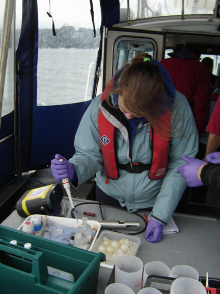 amples were used to fill glass bottles ensuring the
bottles were flushed through with the sample water. Once the samples
were bottled, 1 ml of Manganese Chloride and 1ml of Alkaline Iodide was added to the
bottle to fix the sample. The bottle was then sealed in order to prevent any more oxygen entering the
sample. The bottles were stored underwater until they could be
processed in the lab.
amples were used to fill glass bottles ensuring the
bottles were flushed through with the sample water. Once the samples
were bottled, 1 ml of Manganese Chloride and 1ml of Alkaline Iodide was added to the
bottle to fix the sample. The bottle was then sealed in order to prevent any more oxygen entering the
sample. The bottles were stored underwater until they could be
processed in the lab.
In the laboratory, 3 standards were made to
establish the Thiosulphate normality, which is used to calculate the
oxygen concentration and % saturation of each sample. To each sample 1ml
of sulphuric acid was added and the sample was then titrated. The volume
of Thiosulphate needed to titrate the sample was recorded and the %
saturation could then be calculated. The method used was that according
to Grasshoff et al. (1999).
Chlorophyll
The filters were soaked in acetone overnight to remove the chlorophyll and left in solution. Each sample was decanted into a cuvette and placed in the fluorometer. The reading on the fluorometer was noted, and the following equation was used to convert this value into a total concentration of chlorophyll per litre.
Phytoplankton
The Lugols Iodine samples were placed into measuring cylinders and left overnight to allow the plankton to settle and concentrate the sample. A curve ended tube and vacuum pump was used to remove 90ml of the sample without disturbing the settled plankton, leaving behind a 10ml concentrated solution. These solutions were decanted into labelled bottles, and 1 ml of each sample was placed into Cedric Rafter Cells under the microscope for visual analysis. 10 transects were conducted on the sample noting each species and tallying the species count. This value was then multiplied by 5 to calculate the number of phytoplankton species in 1ml.
Zooplankton
With the two 500ml water samples taken from 2m depth aboard the Bill Conway, and the one from 0.5m depth aboard the RIB Ocean Adventure, 10ml of each was pipetted into an aliquot and studied under a microscope, and duplicated by another person to improve reliability of results. The frequency of various designated zooplankton taxonomic groups was recorded.
Nitrate, Phosphate and Silicate
The methods used to measure silicate and phosphate are stated in Parsons (1984).
The method used to measure nitrate is the Flow Injection Analysis as stated in Johnson and Petty (1983).
Chemical Analysis:
Phosphate
As shown on Figure 2.2, the phosphate concentration in the estuary shows non-conservative behaviour. The diagram shows that the concentration is higher than the theoretical dilution line (TDL) suggesting addition. Inputs of phosphate into the estuary could originate from sewage, agricultural and urban runoff. These effects could have been increased as of result the amount of precipitation which the Falmouth area has recently received.
Nitrate
The nitrate analysis (Figure 2.3) indicates non-conservative behaviour as the data points fall below the TDL, suggesting that there is removal of nitrate from the estuary. Possible reason for this removal of nitrate is uptake by the marine organisms such as phytoplankton and zooplankton. Due to a lack of data caused by time and tidal restrictions no water was sampled at salinities lower than 18.5. It is interesting to note that by excluding the riverine end member, the values of the samples collected appear to plot in a conservative manner.
Silicate
The analysis of the silicate data (Figure 2.4) shows the points in
alignment with the TDL, albeit with some variation, strongly suggesting a conservative behaviour in the
estuary. The values from the marine end member down to a salinity of 24
fall slightly below the TDL and values beyond this plot slightly above the TDL. Processes such as sewage addition or removal via siliceous
phytoplankton may also have an affect, so there
may be some non-conservative behaviour.
Chlorophyll
The chlorophyll
concentration (μg/L) was plotted against salinity to
determine if there was a positive or negative correlation between the
two variables (Figure 2.5).
There was a weak negative correlation with chlorophyll concentration
decreasing with increasing salinity. Chlorophyll levels can be limited
by the variations in the
nutrient concentrations. Nitrate, phosphate and silicate are the vital
components of phytoplankton growth.
However, as surface samples were taken from the upper reaches of the estuary
where the euphotic zone becomes shallower, the phytoplankton were
concentrated higher up the water column. This gave
the impression of an overall higher chlorophyll biomass towards the
freshwater end of the estuary.
The chlorophyll concentrations plotted onto the fluorescence graph were found to have no correlation.
Oxygen
Figure 2.9 shows
that the calculated oxygen saturation falls within a relatively narrow
range, (approximately between 75-85%), with two sets of points lying
outside of this region. The YSI information was recorded at stations by
the RIB and has been calibrated to a high degree of precision. The data
point that lies outside of this field is found at a saturation of 56%.
This was due to a lack of water temperature information from the CTD data,
and as a result the calculated saturation is significantly lower than
the other data.
The oxygen
saturations within the samples are uniform and under-saturated
throughout the estuary, although when compared to the YSI data the
calculated values may be lower than the actual values. Additional
samples would need to be taken in order to establish a more
representative picture of the estuary as a whole.
Biological Analysis:
|
Phytoplankton results
|
Zooplankton results
|
|
Zooplankton Analysis
The proportional bar chart
(Figure 2.7) shows
that Copepoda was the most abundant group at the first station on
Bill Conway, with a calculated percentage of 53. This station was
located closer to the mouth of the estuary than the second station which is dominated by Cirripedia larvae
(barnacles) (52%). Various other groups exist at both of these stations
such as Gastropod larvae, Chaetognaths and Siphonophorae.
At the head of the estuary a
zooplankton trawl was conducted at Malpas Marina and was the most
northern trawl. Only 3 groups were identified within this sample, the
dominant one being hydromedusae (60%). The reason for this may be
due to the various pressures that probably would not exist further down
the estuary, such as the amount of agricultural inputs (fertilizers),
sewage and large salinity fluctuations. Therefore, the zooplankton is
very low in diversity because these groups cannot physically cope with
the stressful environment. Diversity is higher at the stations
positioned closer to the mouth of the estuary where the surrounding
environment is less harsh. Competition lower down the estuary could in
turn decrease diversity, however, the proportional bar charts do not
seem to support this. The groups that have the ability to exist
in low salinities (stenohaline) do not suffer from competition
and therefore, where the diversity is low, the abundance is high.
Phytoplankton Analysis:
The growth of phytoplankton is determined by the amount of available nutrients in the water column and radiation from the sun. These two components are essential in order for the growth and reproduction of phytoplankton. In the summer season, phytoplankton is low in abundance within the surface layers of the water column, and this is due to a lack of available nutrients which have been stripped by the spring bloom. Therefore a large peak of phytoplankton (and hence zooplankton) can be found at the thermocline where nutrients can be regenerated from below and light from the sun can penetrate through the surface layers due to a decrease in mixing and turbidity.
|
Bottle Number |
Latitude |
Longitude |
|
60 |
50o14.689N |
005o01.367W |
|
68 |
50o13.211N |
005o01.601W |
|
61 |
50o12.819N |
005o01.580W |
|
77 |
50o11.713N |
005o02.857W |
|
76 |
50o08.606N |
005o02.382W |
Bottle sample 60 was collected at the top river end (Malpas Point). The main phytoplankton community which was identified here was Nitzschia. This group had a percentage of 64 in comparison with bottle numbers 76 and 77 which had a percentage of 9 and 4 respectively. These two bottle numbers were sampled at the mouth of the estuary and therefore from these results we can determine that Nitzschia survives in a larger abundance in a riverine environment. A possible explanation for this may be due to the higher nutrient abundances generated by agricultural runoff and sewage input from the surrounding area.
The dominant group found in the middle of the estuary was identified as the Chaetoceros species. This was present in bottle number 68 as shown in the table above, and had a percentage of 77. In the same sample other species such as Nitzschia (10.7%), Rhizosolenia setigera (8.9%) and Karenia mikimotoi (3.5%) were also identified. A possible explanation for the net dominance of the Chaetoceros in the middle part of the estuary could be related to its low requirement of silicate.
Bottle sample 76 which was sampled at the mouth of the estuary was mainly dominated by Rhizosolenia delicatala with a percentage of 69.7. Other groups were analysed with much lower percentages such as Chaetoceros (0%), Rhizosolenia stolterfothii (6.57%) and Nitzschia (9.2%). A possible reason for the high dominance of Rhizosolenia delicatala is their tolerance to salinity fluctuations between high and low tide, as well as low nutrient availability.
Physical Analysis:
Secchi Disk Analysis
Figure 2.8 shows that the light
attenuation coeffient, k, increased moving up the estuary due to
increases in turbidity, and the euphotic zone decreased proportionately.
As you move up the estuary the turbidity maximum increases, which will have
an effect upon the light attenuation in the water column due to the
increased number of suspended sediment particles. With an increase in
the light attenuation, the photosynthetic active radiation (PAR) is
limited to the upper regions of the water column, therefore decreasing
the depth of the euphotic zone. This impacts the vertical distribution
of the phytoplankton within the water column.
CTD Analysis
The temperature
profile (Figure 2.15) shows clear thermoclines at all stations, ranging from 2-5m
depth. The surface water temperature increases with distance up the
estuary. There is evidence of stratification from the mouth to the most
riverward point.
In the lower estuary the salinity ranges by no more than 1 unit, while in
the upper estuary there are ranges of 5-7 units. There is greater
evidence of stratification further up the estuary, suggesting a salt
wedge.
Stations 1, 2 and 4 have clear chlorophyll maxima at depths of 2m, 6m and
4m respectively. Stations 3 and 5 have no obvious chlorophyll maxima.
Stations 1, 2 and 3 in the lower estuary have consistently higher
chlorophyll values than stations 4 and 5 in the upper estuary.
There is
greater transmission in the lower estuary, stations 1-3 having values
around 4 volts, suggesting lower turbidity. In the upper estuary
transmission is low, stations 4 and 5 having values of around 1 volt,
indicating high turbidity. At station 2, there is a sharp decrease in
transmission at roughly 16m, from 4 volts to less than 2 volts.
YSI Analysis (Figure 2.13)
Stations 1 to 5 follow the route of the RIB downstream towards the mouth of the estuary and therefore should follow a path of increasing salinity. This is observed to some extent in the data and with the exception of the first station, each successive station downstream is of a higher salinity to the previous one. The first station fits in the middle of the salinity ranges observed which is somewhat of an anomaly but may be a product of the sampling method and unforeseen complications. Due to time restrictions sampling was carried out with the tide instead of against it which may cause some salinity values to be closer together than if sampling was carried against the tide. In addition to this, a fault with the RIB’s alternator delayed us at station 1 for such a time that a significant fraction of the water may have flooded past us on the ebb tide and so when we collected samples at the next station we may have been sampling water previously further upstream that we were at the first station.
The temperature graph shows that temperature (oC) decreases with depth at all of the 5 stations sampled. There is no evident thermocline present in the YSI record which suggests a partially mixed estuary. Temperature is highest in the middle stations and the two lowest surface temperatures are found at stations 1 and 5. This may be a product of possible anthropogenic inputs in the middle of the upper estuary. Station 5 displays a colder temperature profile in comparison to the other profiles. A possible explanation for this may be because this station is situated the farthest seaward, and therefore contains a higher amount of colder, more saline water.
There is a lot of noise present within the turbidity profile. The YSI record shows that the turbidity is higher at the head of the estuary (station 1) and a possible explanation for this could be due to the runoff and agricultural inputs from the surrounding land and area. At this station we were positioned at the nodal point of Truro River and Tresillian River, meaning that a high load of particulate matter was present, shown by the raised turbidity parameter.
The turbidity is lower near the mouth of the estuary and a probable explanation for this is that at the top of the estuary the river is more restricted, so further seaward, as the channel widens, the particulate content is spread through a larger volume of water.
The pH profiles for each station show a progressive increase in pH as the mouth of the estuary is neared. The pH does not fluctuate greatly with depth at any of the sampled stations.
The chlorophyll profile shows a lot of noise and therefore it is very difficult to analyse. The chlorophyll concentration is similar at all the stations where samples were taken.
In the O2 profile the amount of O2 present at the
surface decreases progressively with depth at each station. O2
values increase towards the mouth of the estuary.
ADCP Analysis
STATION 3
The transect between Trefusis Point and St. Mawes Castle passed across the deep shipping channel found running through the Falmouth Estuary. Note that the ADCP was not set up to read data below 14m depth, hence the missing data. The velocity is fastest in the central channel and in the closely surrounding waters at 0.3m/s, whilst the shallower water has flow velocities slowing to about 0.2m/s and below. Flow direction appears to be constantly uniform as a result of the ebbing tide. Backscatter peaks at about 3-4m almost consistently throughout the transect, with the remainder of the water body having a lower backscatter, suggesting the presence of particulate matter. CTD fluorescence data depicts a slight chlorophyll peak at about 4m, and this could correspond to the high backscatter seen on the ADCP. Richardson Numbers calculated from this transect show a relatively stable water column, apart from the surface waters when the Richardson Number drops to just above 0. Surface instability is a result of wind stress acting just on the surface layer.
STATION 4
This transect
was carried out across the Fal Estuary just to the south of Restronguet
Creek. A clear division between upper and lower layers within this
region is present. Flow velocity is greatest in the bottom layer, with
slower velocities up to about 9m. The two layers travel in opposite
directions, with the lower, salty dense layer travelling upriver and the
fresher upper layer travelling seaward. This separation between dense
and less dense waters can lead to the classification of a partially
stratified estuary. Backscatter shows a prominent surface layer
indicating the presence of particulate matter within the freshwater
layer. This is a result of fluvial run-off importing sediments into the
water.
There
appears to be a consistent boundary at just under 6m in both the average
backscatter and velocity direction, apparently corresponding with the
drop in the chlorophyll values. A stable water column until about 7-8m
is observed, at which point a drop in the Richardson Number occurs
representing instability of the water body
Discussion
The investigation of the Falmouth estuary has enabled us to determine that all nutrients such as nitrate, phosphate and silicate have a higher concentration between salinities of 20 and 30. Concentrations are higher toward salinities of 20 and decrease progressively to the mouth of the estuary.
Phytoplankton and zooplankton communities were analysed from samples taken at various depth. The main following species were found:
- Zooplankton: Copepoda
- Phytoplankton: Nitzschia; Chaetoceros spp; Rhizosolenia delicatula.
The regular diurnal fluctuation in salinity enables only euryhaline species to survive, although it also means less competition where there is lower diversity and higher nutrient concentrations due to runoff from agricultural waste and sewage in the Falmouth area.
Studying the chlorophyll concentrations has shown that the depth of the thermocline as well as nutrient concentrations determines the depth of the chlorophyll maxima. The light attenuation coefficient k increased as we moved up the estuary as a result of higher turbidity and particle suspension with mixing in the upper estuary. Finally the oxygen saturation remained under-saturated throughout the estuary at 75-85% according to laboratory analysis.
Turbulent mixing prevents the development of a thermocline and stratification only occurred at stations that were statically stable. A two layer flow appears to be present in the estuary with cold, dense seawater underlying fresh water. However, as the ADCP surveyed only to 14m depth water flow below this, in particular the channel, has not been studied and therefore a true water column structure cannot be determined.
A chlorophyll maxima is present at both stations 3 and 4, but the overall concentration at station 4 is lower because of its proximity to Restronguet Creek, which is known to be a source of heavy metals and contaminants. This pollution creates a more hostile environment and the diversity and abundance of species is likely to be decreased.
Transmission dramatically increases upriver indicating an increase in turbidity, and this could possibly explain the chlorophyll difference between 4 and 5, and 1, 2 and 3.
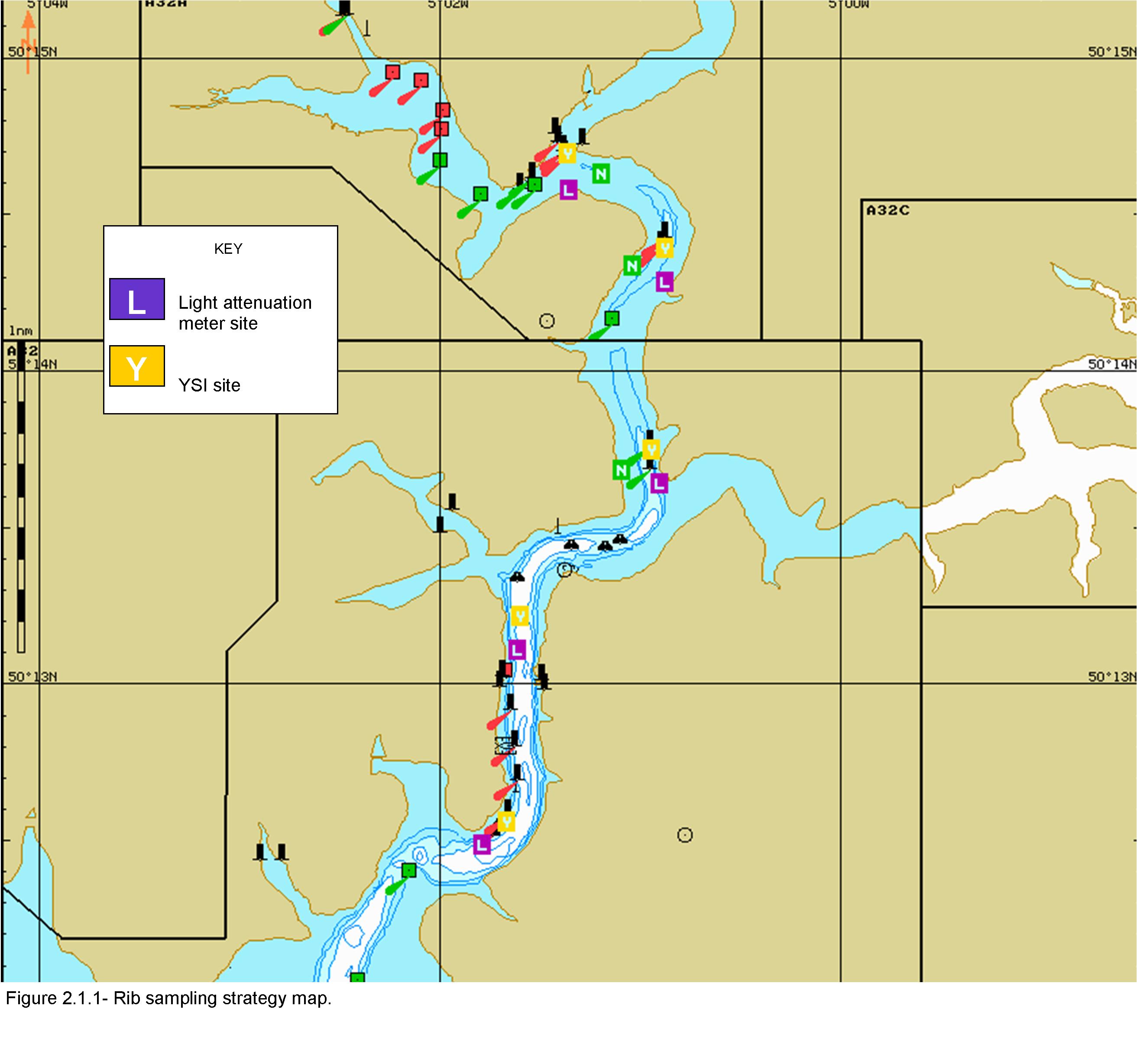
Figure 2.1.1 - RIB Sampling Strategy &
Location
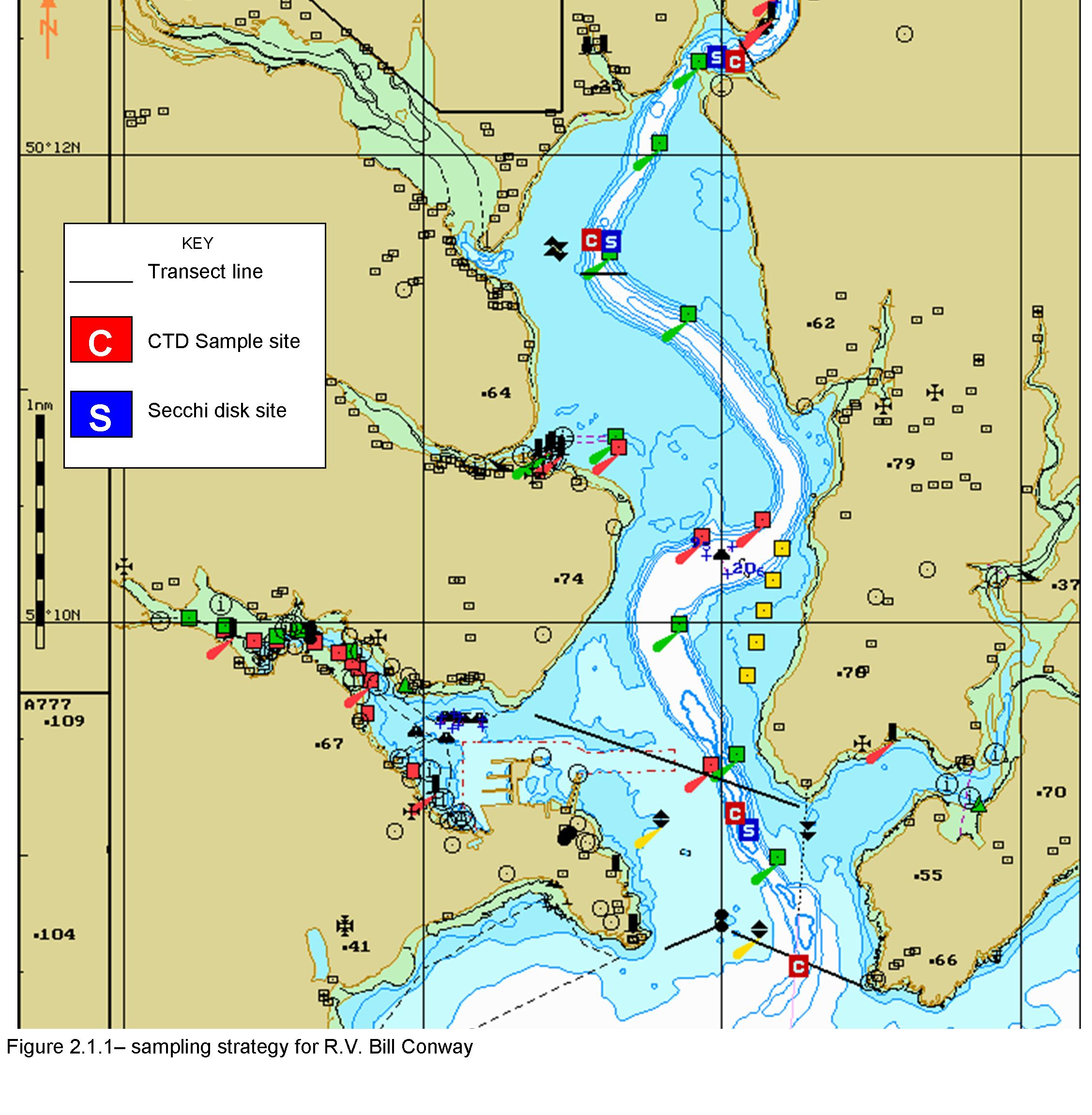 Figure 2.1.2 - Conway Sampling Strategy &
Location
Figure 2.1.2 - Conway Sampling Strategy &
Location
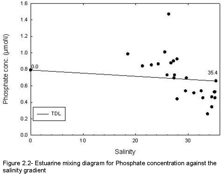
Figure 2.2 - Phosphate
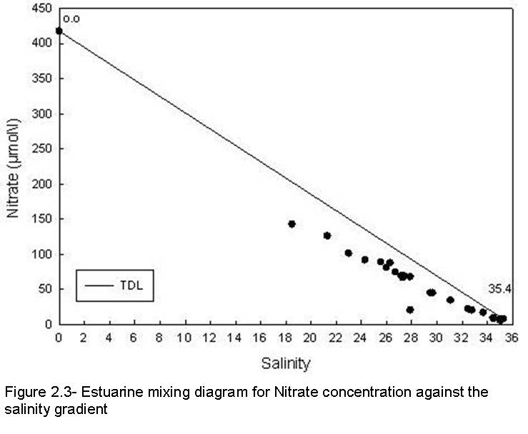
Figure 2.3 - Nitrate
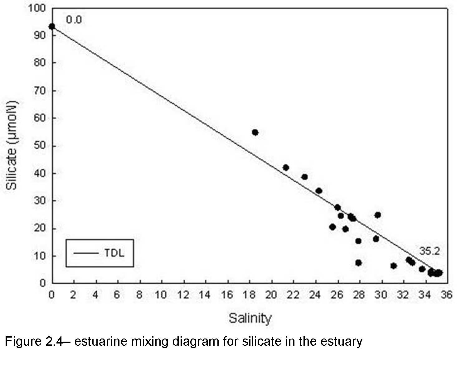
Figure 2.4 - Silicate
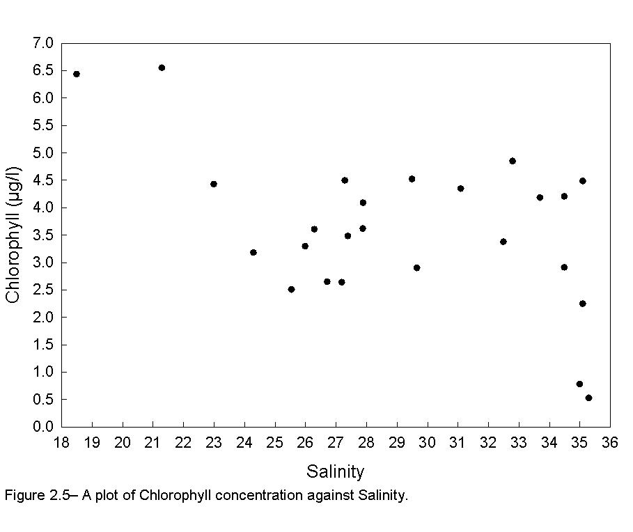
Figure 2.5 - Chlorophyll
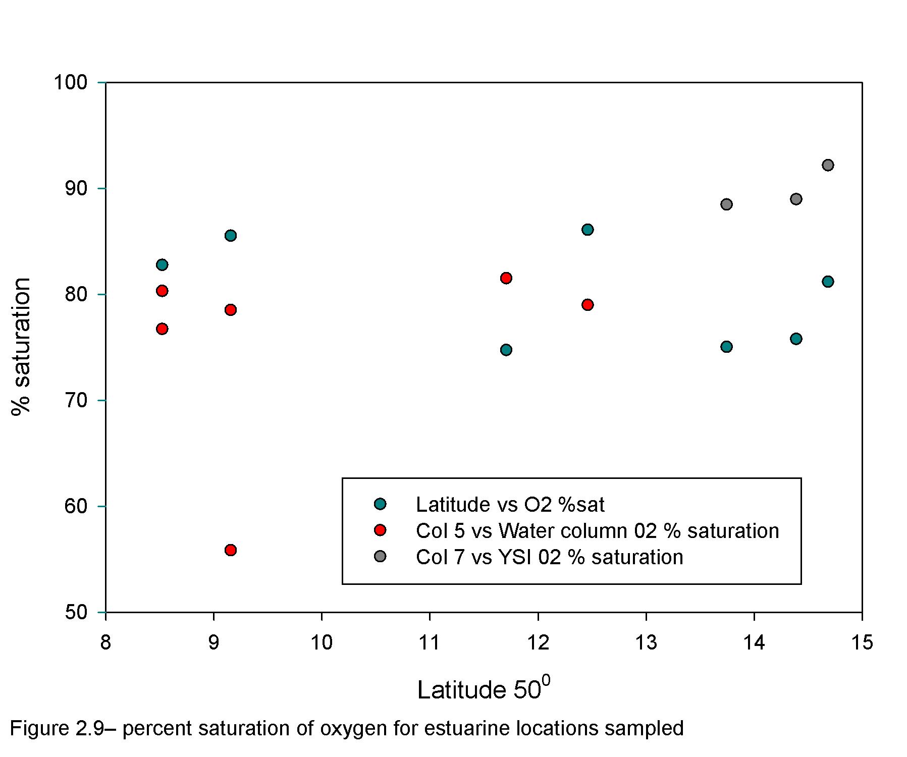
Figure 2.9 - Oxygen
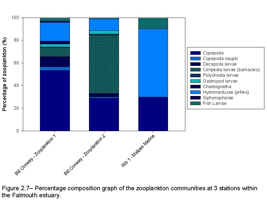
Figure 2.7 - Zooplankton
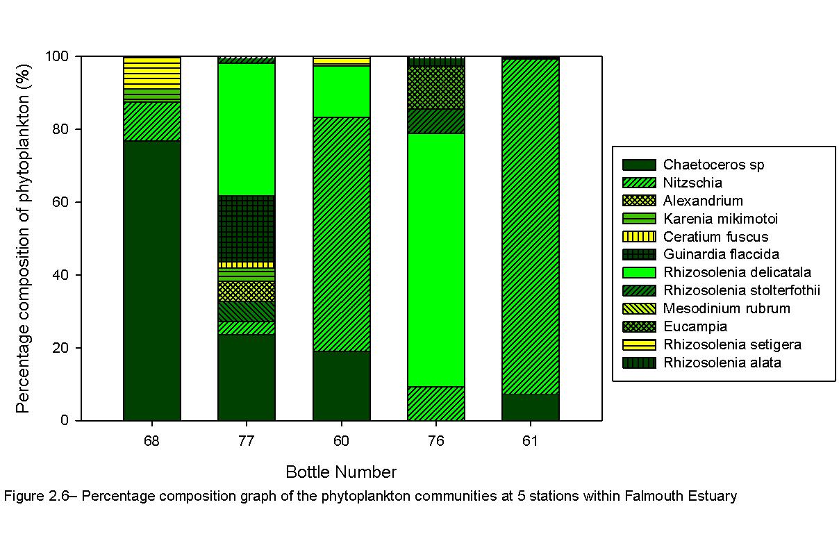
Figure 2.6.1 - Phytoplankton
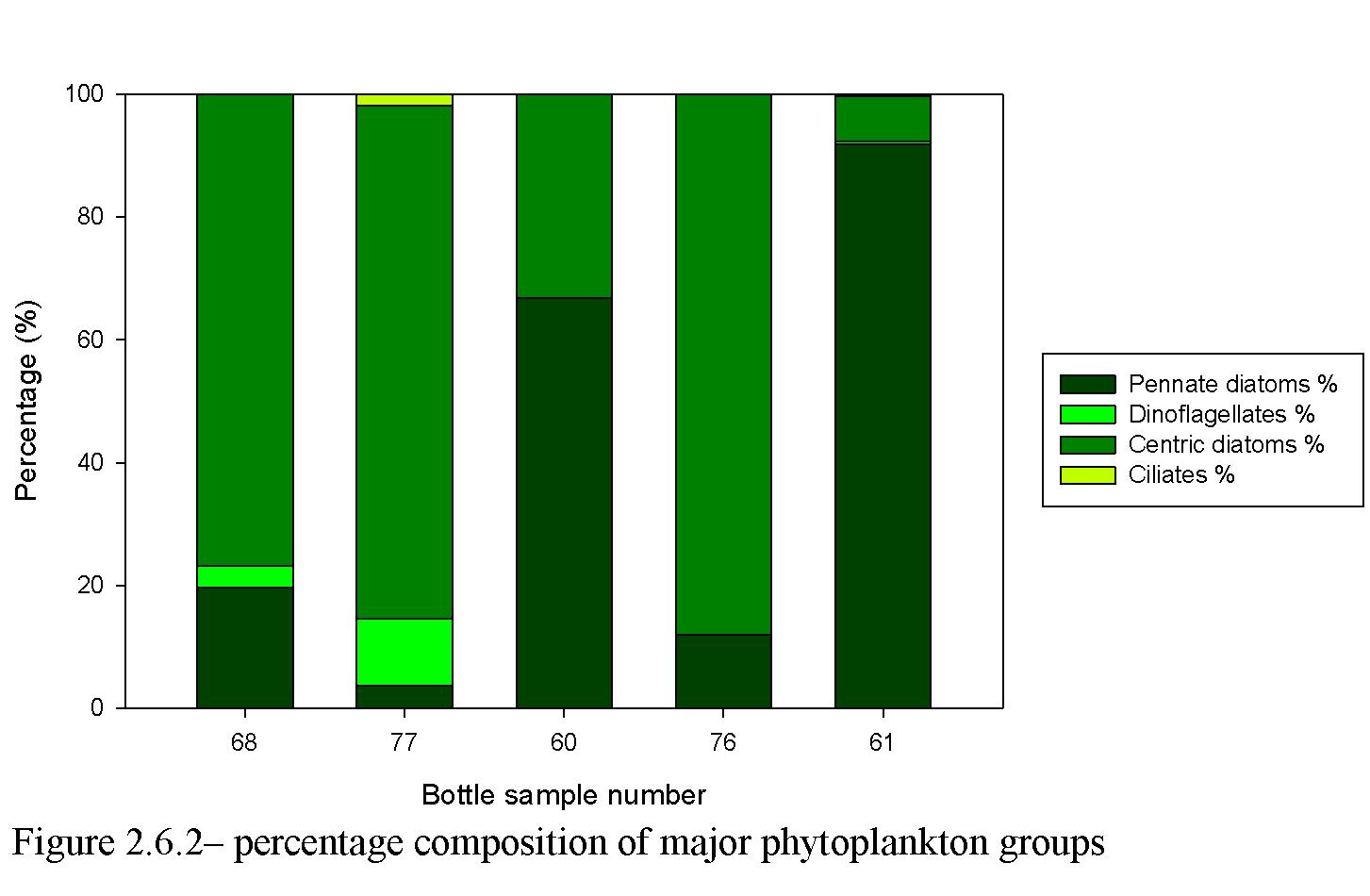
Figure 2.6.2 - Main phytoplankton groups
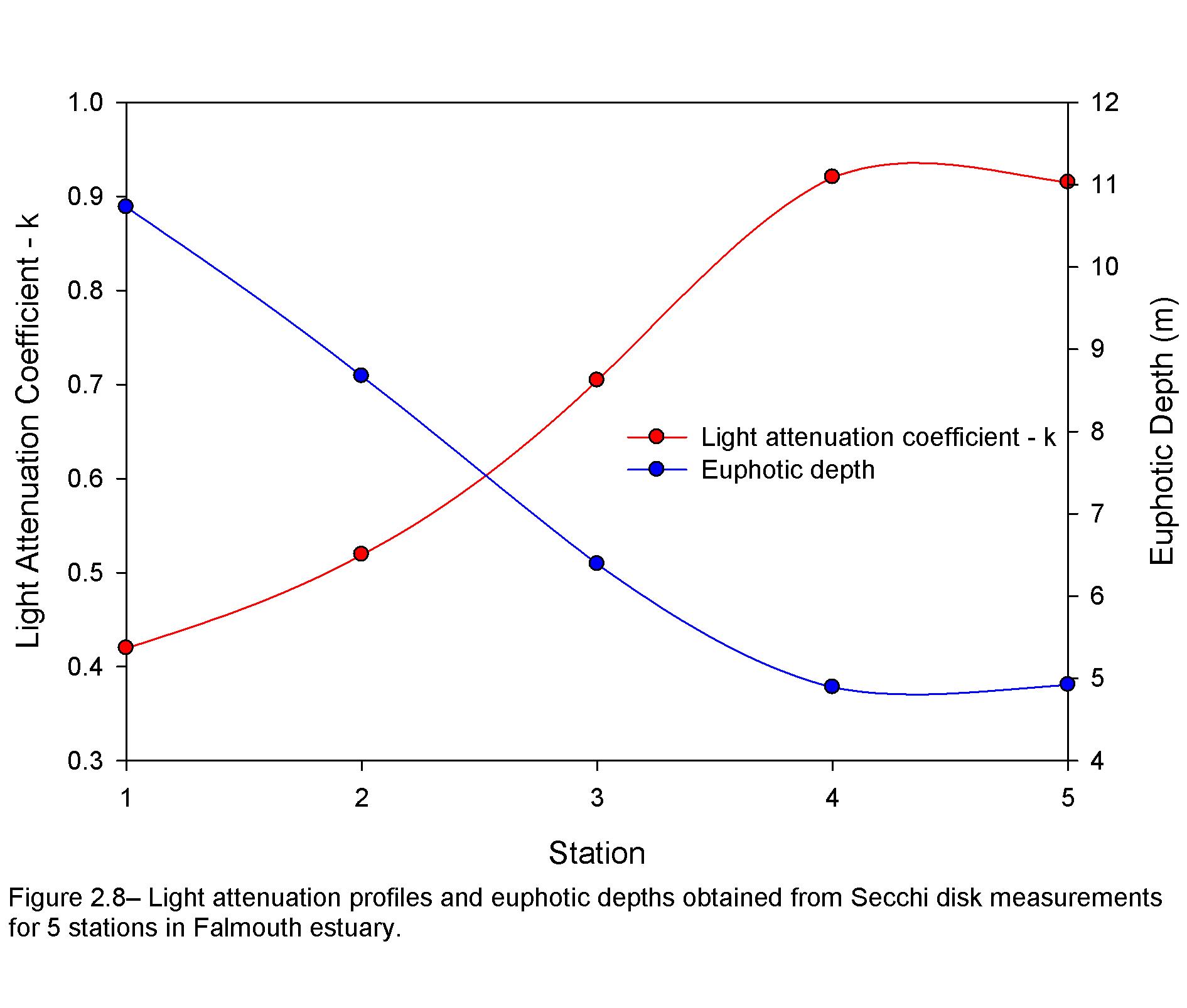
Figure 2.8 - Secchi Disk
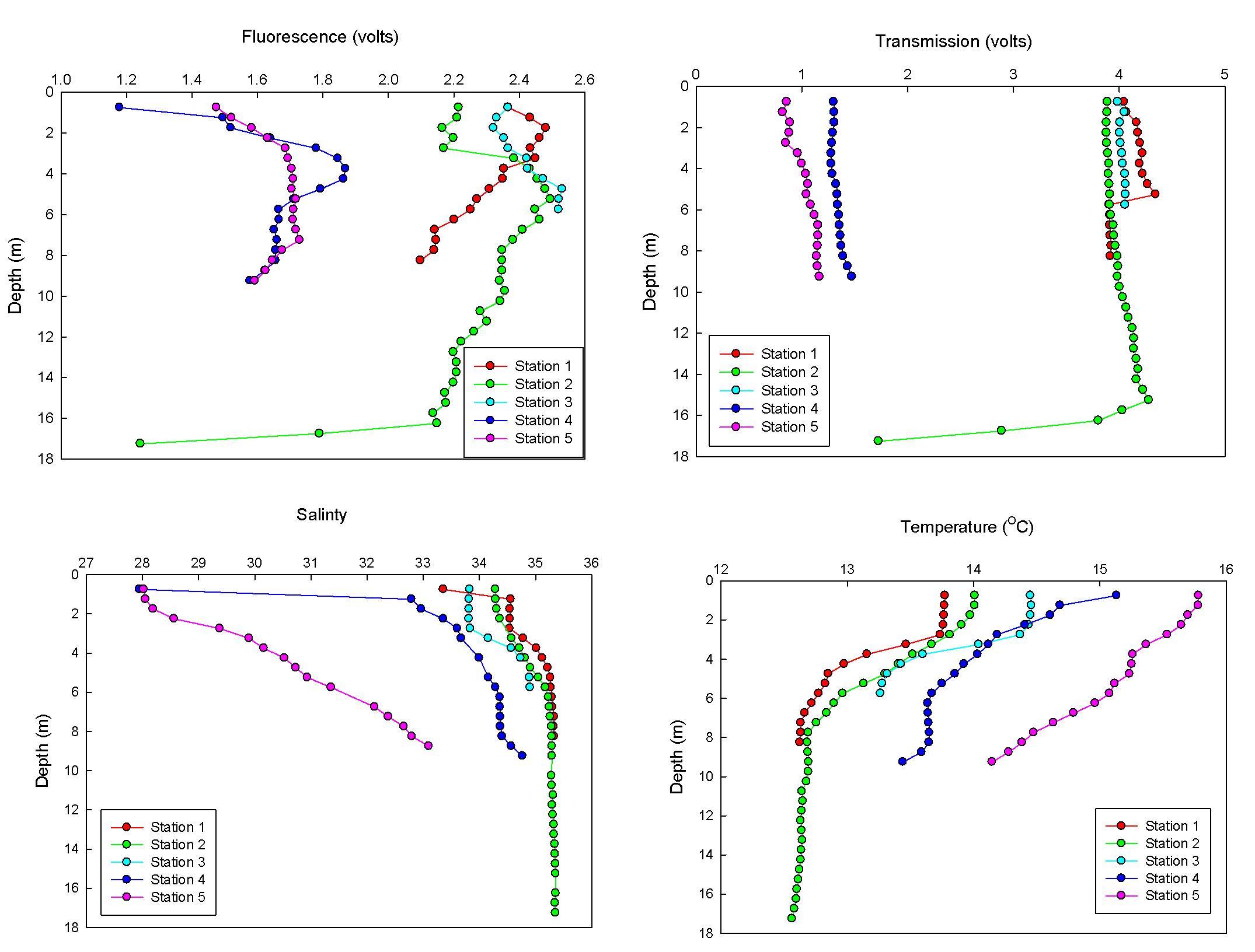
Figure 2.15 - CTD data
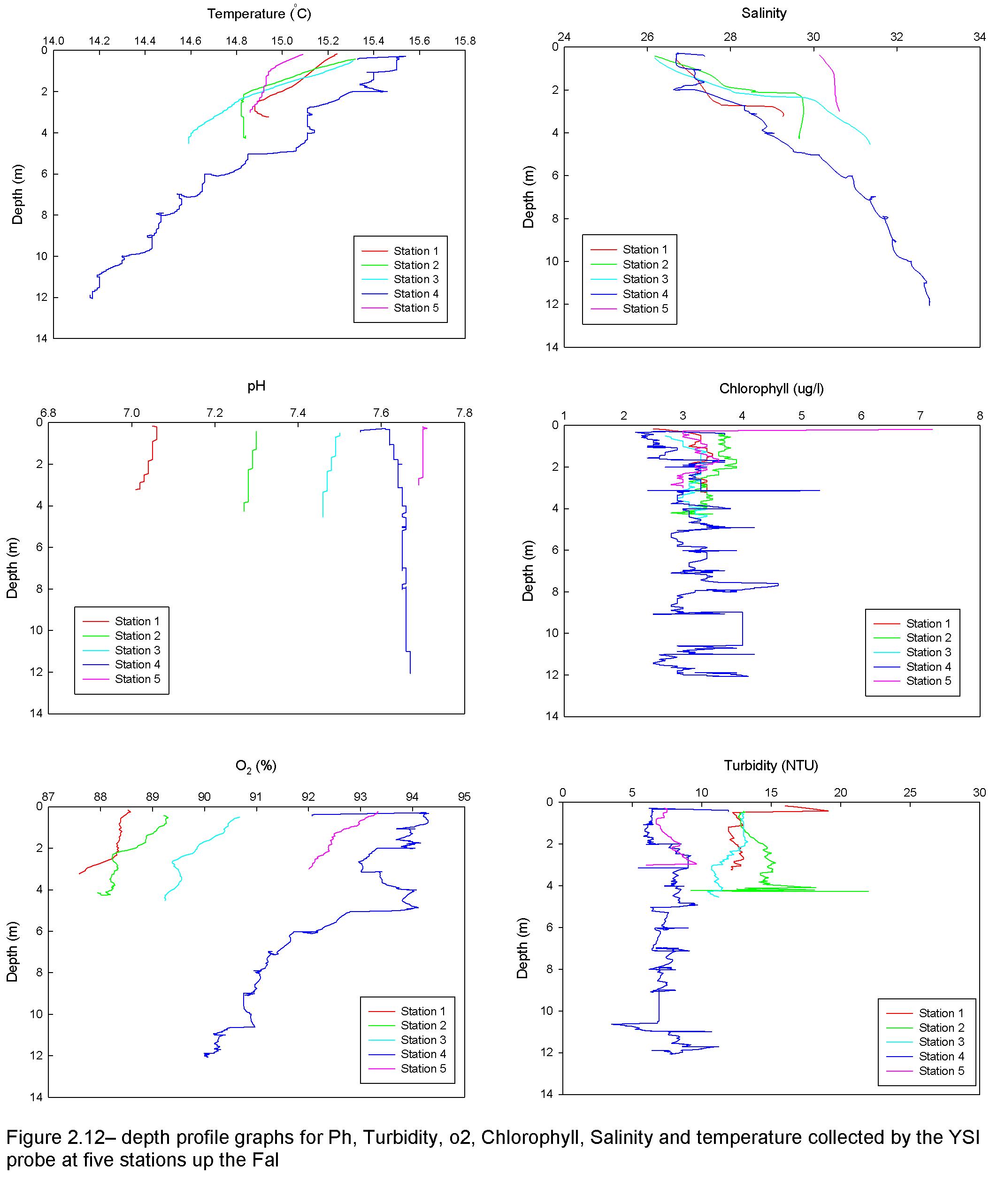
Figure 2.13 - YSI
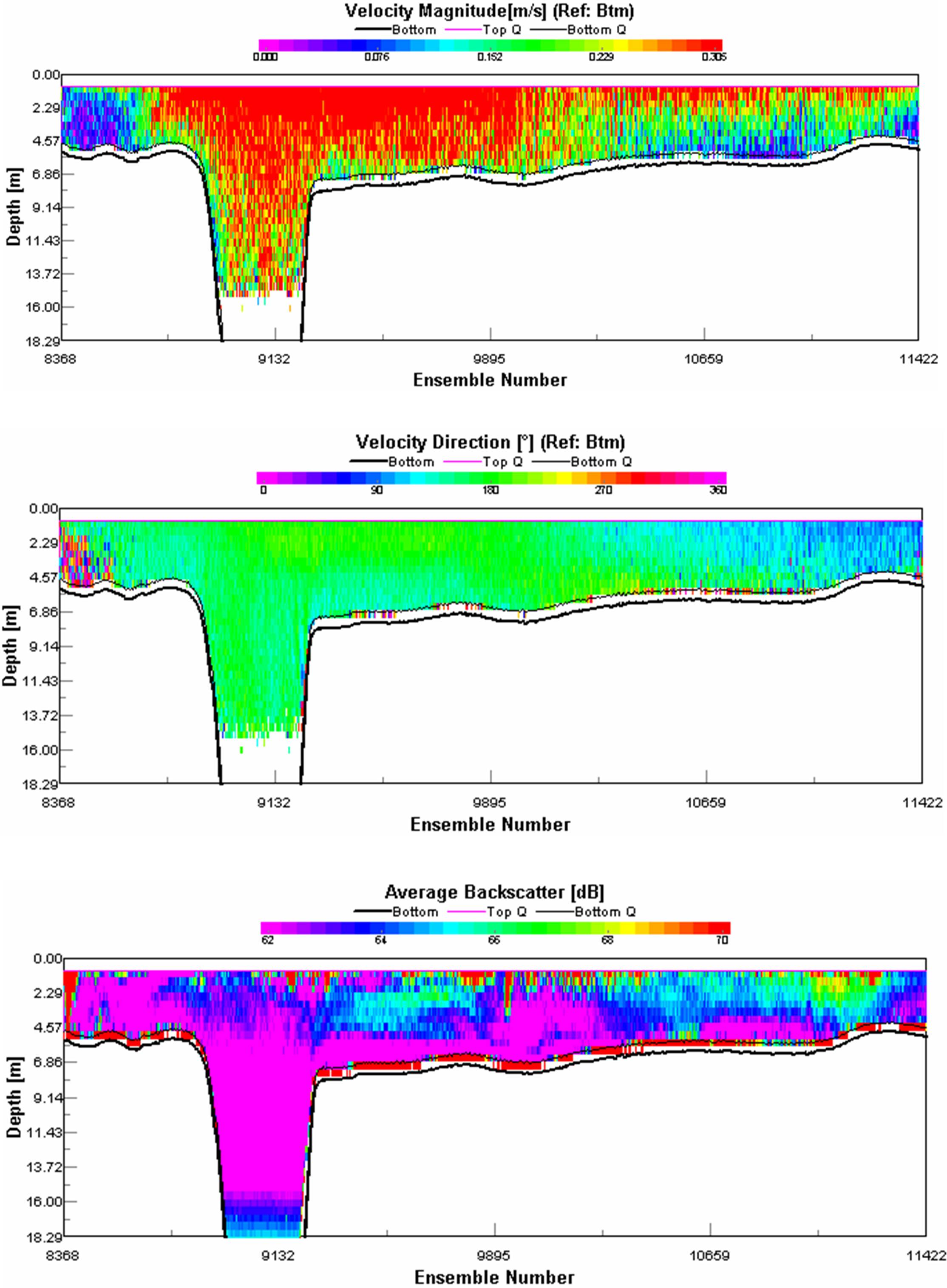
Figure 2.10 - ACDP
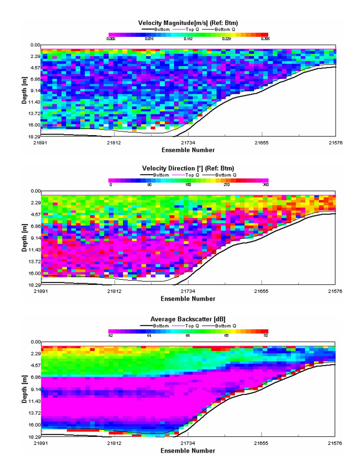
Figure 2.11 - ACDP
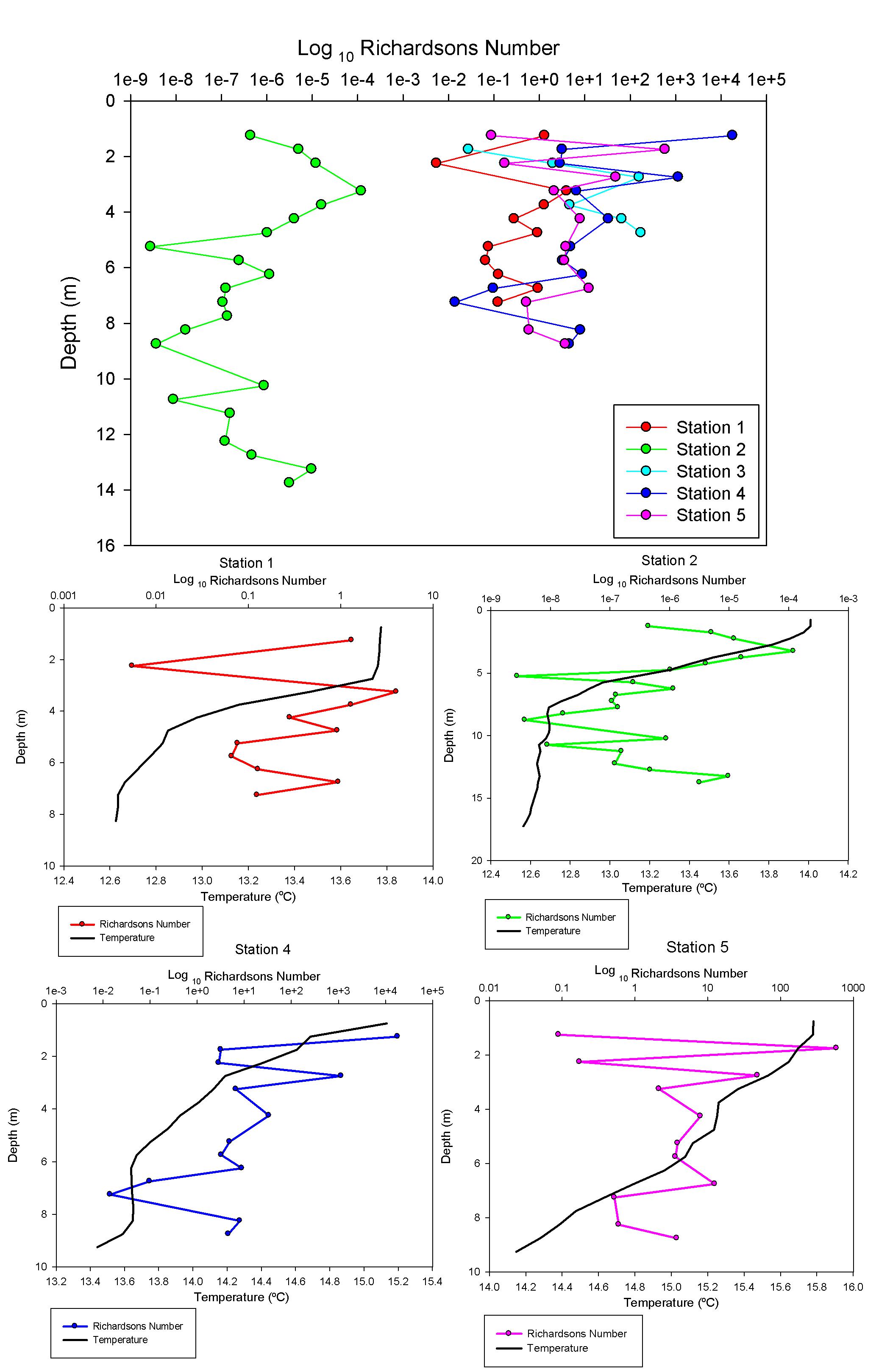
Figure 2.14 - Richardsons number plot
Offshore - 6/7/07 - Day 4
NAVIGATION
Aims:
To investigate the vertical mixing of the water body and its biological processes off shore of Falmouth.
Further analysis will be made to investigate from the the mouth of the estuary to offshore and observe how nitrate, phosphate and silicate concentrations change with depth. Information is also to be collected on dissolved oxygen concentration and quantitative and qualitative measurements of the phytoplankton and zooplankton communities. Samples will also be taken offshore to determine the location of the front and compare it to the lower reaches of the estuary.
Objectives:
-
To sample the lower reaches of the estuary and the offshore of Falmouth at a sufficient number of stations.
-
To assess the non-conservative or conservative mixing behaviour of nitrate, phosphate and silicate from the mouth of the estuary to offshore of Falmouth.
-
To assess the vertical mixing of phytoplankton and nutrients throughout the water column at various stations.
-
To quantify and identify the phytoplankton and zooplankton communities present at different sampling stations.
-
To carry out transects in order to assess the current velocities and particle concentration within the water column surrounding Falmouth and the lower reaches of the Fal estuary.
-
To determine the light attenuation coefficient.
Complications:
-
Due to heavy force winds (approximately force 9) in the offshore regions of Falmouth, decisions were made to cancel the plan and therefore we followed our alternative sampling strategy. This was to study the vertical mixing of the water column in the Falmouth bay and the Helford estuary. We followed the same procedures had we been offshore.
-
Other complications included not recording the ADCP (Acoustic Doppler Current Profiler) and the CTD (Conductivity, Temperature and Density) rosette data simultaneously. Therefore, when analysing the data collected it could give limitations to our final results.
Sampling Strategy:
|
Station Number |
Latitude |
Longitude |
Time (GMT) |
|
Station 1 |
50o08.631N |
005o02.424W |
0850 |
|
Station 2 |
50o08.501N |
005o02.433W |
1016 |
|
Station 3 |
50o07.856N |
005o04.150W |
1033 |
|
Station 4 |
50o06.006N |
005o04.798W |
1112 |
|
Station 5 |
50o05.740N |
005o09.022W |
1226 |
|
Station 6 |
50o05.709N |
005o09.190W |
1245 |
|
Station 7 |
50o05.842N |
005o07.480W |
1325 |
|
Station 8 |
50o05.798N |
005o06.106W |
1344 |
|
Station 9 |
50o07.880N |
005o04.018W |
1408 |
|
Station 10 |
50o08.406N |
005o01.591W |
1458 |
Tides and Weather:
|
|
Time (GMT) |
Depth (m) |
Weather: |
|
1st Low Water |
0315 GMT |
1.1m |
Sunny with a maximum temperature around 18-19oC. Inshore wind strength was recorded at 4-5 force, however, due to extremely strong wind conditions (approx. force 9) our group was unable to venture offshore. |
|
1st High Water |
0909GMT |
4.7m |
|
|
2nd Low Water |
1531GMT |
1.3m |
|
|
2nd High Water |
2120GMT |
5.0m |
Equipment:
|
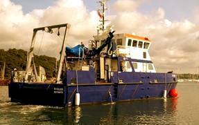
R.V. Callista - Offshore & Helford Estuary |
| CTD & frame inc. rosette of Niskin bottles (labelled FS2aa - FF2ag) (GO - General Oceanics), a transmissometer (F38-C), fluorometer (F38-F) and a light attenuation meter. |
| 2x pipettes which held a standard 1000ul- VOLAC |
| ADCP with WINRIVER - ADCP software system |
| Water bottles (glass for phosphate and nitrate samples, plastic bottles for silicate samples) |
| Closing zooplankton net (200um) |
| Cool box |
| Secchi Disk |
| Plastic tubing for transferring oxygen samples into labelled glass bottles |
| Plastic test tubes (all labelled) |
| Lugols iodine (phytoplankton) & Formalin (zooplankton) |
| Plastic syringes |
| Winker Reagent |
| Map chart - NAVIFISHER |
PSO: Jennifer Wright
Equipment procedures:
Procedures were the same as for aboard the R.V. Bill Conway. See
here.
However there are different safety protocols onboard the Callista for deploying equipment which are outlined below.
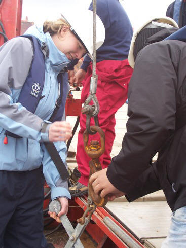
 Prior to deployment of the CTD rosette,
before arriving at a station, or in between casts, each Niskin bottle
(attached to points 2,4,6,8, and 12 on the rosette) is opened at both
ends and secured in position. Upon arrival at a station, permission to
deploy equipment is requested from the skipper and pending an
affirmative response, two handling ropes are fed under the metal bars of
the CTD rosette to prevent the rig swinging dangerously during hoisting
off the deck and into the water. At this point hand signals are
communicated to the winch operator at the stern of the top deck to raise the CTD
to move it
out over the water and lower it to the surface.
Prior to deployment of the CTD rosette,
before arriving at a station, or in between casts, each Niskin bottle
(attached to points 2,4,6,8, and 12 on the rosette) is opened at both
ends and secured in position. Upon arrival at a station, permission to
deploy equipment is requested from the skipper and pending an
affirmative response, two handling ropes are fed under the metal bars of
the CTD rosette to prevent the rig swinging dangerously during hoisting
off the deck and into the water. At this point hand signals are
communicated to the winch operator at the stern of the top deck to raise the CTD
to move it
out over the water and lower it to the surface.
When the recovery to deck order is issued,
the winch
man will raise the CTD to the surface. The deck crew then use pole devices that hook carabinas on the
end of ropes to the yellow rig, wrapping their end of the rope around a
bollard on the beam that again ensures the safety of the crew against
the CTD rosette swinging as it is then raised and brought carefully on
to the equipment stage. At this point the water
samples were collected from the Niskin bottles and prepared
for the next cast.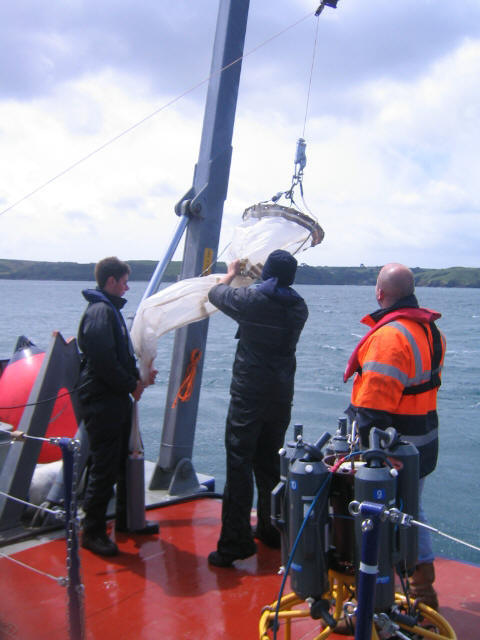
The other piece of equipment to be deployed from the equipment stage was the vertical
closing zooplankton net (mesh size 200μm, opening area 50cm). When the net
reaches the bottom limit of the chosen section of water column to
sample, it is then steadily raised to top limit of the section,
whereupon a messenger is attached to close the net. The plankton are washed
down the net using the deckwash hose. The sample is washed into a plastic sample
bottle.
Experimental procedures:
Procedures were the same as for
samples collected on the estuarine survey. See
here
Chemical Analysis:
A strong relation can be observed between all three nutrients, especially nitrate and silicate. This can be observed in Figure 3.2.1, 3.3.1 & 3.4.1 where only the surface measurements are plotted and an almost linear decrease in nutrient concentration is observed alongside increasing salinity.
Nitrate
The Nitrate plot (Figure 3.2) shows a strong correlation between values giving some indication of how strongly linked the abundance of these nutrients are in the water column. Nitrate is found at its lowest concentration near Black Rock, and then values increase slightly with distance out to sea and up the Helford Estuary. Some of the highest values are found up the Helford Estuary where inputs from sediment run-off and anthropogenic sources may be increasing this value. This is similar to the results of the Fal estuary during the estuarine sampling. Interestingly, sites towards the mouth of this estuary, while having the highest nitrate levels had much fewer phytoplankton, while the Black Rock sample with the lowest nitrate has some of the highest phytoplankton counts.
Phosphate
Phosphate (Figure 3.3) is found in consistently small values ranging from 0.2-0.3μM and it is possibly the limiting nutrient at some of these near offshore sites. The surface values for phosphate were similar to silicate and nitrate, but showed more variation than either of these possibly due to the accuracy of measuring these small values or variation in the input of phosphate from sources higher up the estuary.
Silicate
Silicate (Figure 3.4) concentration varies between 2 – 10 μM. The variation at sites once again can be linked inversely to the quantity of phytoplankton found at these sites. The strong correlation between silicate and nitrate suggests that the majority of the phytoplankton must be using silicate albeit at a different scale alongside nitrate. If this is the case as observed we would expect the majority of the phytoplankton to be silaceous which is backed up by observing the dominance of diatoms found in the phytoplankton samples.
Chlorophyll
We plotted chlorophyll concentration against salinity and found no correlation between the two variables. In the offshore waters, there is negligible difference in salinity, and the phytoplankton in these waters are no longer limited and distributed by salinity. Their new distribution is determined by micro-habitat nutrient availability, the depth of the euphotic zone, and the depth of the thermocline in accordance with the offshore frontal systems. Once again the chlorophyll concentrations at depth were plotted onto the fluorescence plot and were found to have no correlation.
Oxygen
The data that was collected in the Helford River is plotted in
Figure 3.9, giving the opportunity to study how the oxygen saturation
changes as we moved seaward. The data that was not plotted was sampled
from positions in Falmouth Bay and from the entrance to the Fal Estuary.
These stations were located at a considerable distance apart and as a
result drawing any firm conclusions would be near impossible.
Figure 3.9 shows that there is a decrease in saturation percentage travelling towards the river mouth. This is contrary to what we would expect, although the range in recorded values is only over a range of 8%, which is an indication that the oxygen is uniform in its structure throughout the transect and that there is only minor deviation between values taken in surface samples when compared to ones taken at depth. Samples taken at regular intervals may help to establish if a significant difference exists between different points in the estuary.
Biological Analysis:
|
Plankton results
|
Zooplankton
results
|
|
Plankton
Analysis:
The growth of phytoplankton
is also determined by the amount of available nutrients in the water
column and radiation from the sun. For more information see Figure
3.6.1
and 3.6.2.
|
Station Number |
Latitude |
Longitude |
|
1 |
50o08.376N |
005o01.430W |
|
4 |
50o05.957N |
005o04.692W |
|
6 |
50o05.681N |
005o09.216W |
At station 1 (Black Rock) two samples were made, one at the surface and another sample at 5m depth. The sample taken at the surface showed a high concentration of centric diatoms with a percentage of (90%) with very low concentrations of dinoflagellates, pinnate diatoms and ciliates. The following sample at the same location also showed that centric diatoms dominate the water column at 5m depth. Station 4 also had in its sample very high concentrations of centric diatoms. Finally, station 6 showed some differences in the composition of the phytoplankton community in the water column. There was a dominance of ciliates (50%) and centric diatoms (45%) in comparison to a low concentration of pennates and dinoflagellates in the same sample. This could be due to a change in nutrient availability, an increase in heavy metals and anthropogenic inputs such as sewage.
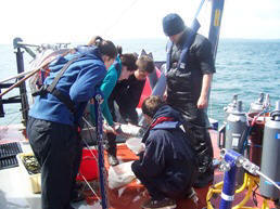 Figure 3.6 shows the taxonomic
zooplankton identified at each sampling station and at various depth
ranges. It can be seen from the graphs that the Copepoda group
was the most abundant at every station that was sampled. At stations 1
and 4 Copepoda was found in a higher concentration in the shallow
water than at depth. At station 1 Copepoda contributed 77%
between the depths of 15m and 5m and 91% at station 4 between the depths
of 5m and 0.5m. At the same stations Copepoda were
recorded as 54% and 63% at depths of 23.9m-15m and 10m-7m respectively.
There are a relatively large number of Copepoda nauplii and a
possible reason for this maybe because of the closeness of the mussel
farm which act as a source of eggs to the surrounding area. Also, the
estuary was sampled on a spring tide which is the period when fish tend to
broadcast spawn, giving them a better chance of
surviving. This suggests why there is a relatively large abundance of
Copepoda nauplii identified in our samples. At stations 4 and 9
Copepoda also dominate the samples with more Copepoda being found in the
surface waters and station 4 (91.2% between 6m and 0.5m in comparison to
63%). A relatively large abundance of Copepoda nauplii have also
been identified at depth in all of the stations in comparison to depth.
There is also a higher diversity of groups at depth.
Figure 3.6 shows the taxonomic
zooplankton identified at each sampling station and at various depth
ranges. It can be seen from the graphs that the Copepoda group
was the most abundant at every station that was sampled. At stations 1
and 4 Copepoda was found in a higher concentration in the shallow
water than at depth. At station 1 Copepoda contributed 77%
between the depths of 15m and 5m and 91% at station 4 between the depths
of 5m and 0.5m. At the same stations Copepoda were
recorded as 54% and 63% at depths of 23.9m-15m and 10m-7m respectively.
There are a relatively large number of Copepoda nauplii and a
possible reason for this maybe because of the closeness of the mussel
farm which act as a source of eggs to the surrounding area. Also, the
estuary was sampled on a spring tide which is the period when fish tend to
broadcast spawn, giving them a better chance of
surviving. This suggests why there is a relatively large abundance of
Copepoda nauplii identified in our samples. At stations 4 and 9
Copepoda also dominate the samples with more Copepoda being found in the
surface waters and station 4 (91.2% between 6m and 0.5m in comparison to
63%). A relatively large abundance of Copepoda nauplii have also
been identified at depth in all of the stations in comparison to depth.
There is also a higher diversity of groups at depth.
Pie charts were created in order to show diversity and abundance at each
station and at different depths. This method enables the diversity and
abundance to be compared at different depths in order for valid
conclusions to be made. By counting the number of groups in a 15ml
sample we were able to calculate the number of groups per m3.
This was done by dividing the number of groups in the 15ml sample by 15
and then multiplying by 500ml. This calculated the volume of the bottle
that the sample was collected in. In order to determine the volume of
water that passed through the zooplankton net the following formula was
used:
Volume= π x r2 x height (the difference between the depth that the zooplankton net opened and closed)
The
diameter of the zooplankton closing net was recorded as 59cm and
therefore the r2 could be calculated.
The number of groups in 500ml was then divided by the volume of water
that passed through the zooplankton net between recorded depths in order
to give the number of groups per m3.
The zooplankton trawl at station 1 was taken at Black Rock which is
positioned at the mouth of the Fal estuary. There were two trawls taken
at two different depths at each station. By looking at the pie charts we
can see that between the depths of 23.9m and 15m there are fewer
Copepoda in comparison to that at a shallower depth range of
15m-5m. However, the diversity of groups is higher at depth and the
abundance of each group is more evenly distributed. Copepoda are
the most dominant zooplankton group with 1317 groups in a m3
at depth and 3602 species in a m3 in shallower waters.
Station 4 was positioned SE of August Rock, near to the entrance of the
Helford River. In this position Copepoda were found to be the
dominant group at both of the depth ranges sampled. Again, there were
a larger number of Copepoda per m3 (9634) in the
surface water in comparison to at depth (1870). The diversity of groups
is very similar in both of the sampled depth ranges, however, in the
surface we can see that Copepoda make up the majority
of the sampled water.
In the
Falmouth Bay area (station 9) there is a higher recorded diversity of
groups in the surface than at depth. Again, as has been seen before,
Copepoda have the highest recorded abundance, however, other
groups
such as hydromedusae and gastropod larvae were also
identified, but in lower proportions. The number of Copepoda per
m3 in the surface was higher than at depth, as can be seen at
the other stations. At all of the stations sampled there was a much
higher abundance of groups, but a higher diversity at depth, excluding
station 9, where there was a higher diversity of groups at the surface.
Physical Analysis:
Secchi Disk Analysis
Figure 3.8 of the Callista Secchi Disk data
shows the light attenuation
coefficient k and
euphotic zone depth calculated from
Secchi Disk depths
recorded at Black Rock, to the upper Helford estuary, and the return
voyage to Black Rock. Again this graph shows an inversely proportional
relationship between light attenuation and euphotic depth. The k
value was greatest in the upper Helford estuary at 0.498 as a result of
the increase in turbidity associated with estuarine mixing and particle
suspension. The lowest k value, 0.187, was determined at the mouth of
the Helford estuary.
CTD Analysis
Thermoclines are present at stations 9 and 10, the most seaward of our
sampling stations. The thermoclines develop between 5 and 10m depth,
ranging in temperatures from 12.8˚ C
to 14˚ C.
At stations 1, 2, 3, 4 and 9 there are no haloclines present, whilst at
station 10 there is a prominent halocline at a depth of 6m.
At stations 1, 2, 3, 4, 8 and 9 there is no change in transmission with
depth other than minor fluctuations. Station 10, on the other hand,
shows a prominent increase of 0.4 volts between the surface and depth.
A peak of fluorescence from approximately 1 to 3 volts exists at
stations 1, 3, 9 and 10 suggesting the chlorophyll maxima exist at
roughly 8m.
Thermosalinograph Analysis
The thermosalinograph continuously recorded
temperature and salinity throughout the survey. The plot shows data
between 50° 08.631N, 005° 02.424W and 50° 05.676N, 005° 06.095W,
corresponding with our survey of the Helford estuary and Falmouth Bay.
The data shows a steady decrease in temperature with increase in
salinity, with a decrease of about 2°C between a salinity of 31 and 35.
ADCP Analysis
STATION 6
The transect along the Helford River passed through
The Pool reaching to a depth of 15 metres, whilst the CTD at station 6
was found further upriver of this. The magnitude of the velocity appears
to fluctuate throughout the water column with a general velocity of
0.2m/s with a maximum of 0.6m/s. The direction of velocity is generally
down river, related to the ebbing tide at the time of the transect.
Average backscatter is relatively high and uniform at Station 6,
explained by its location upriver. The high levels of matter within the
water column are due to the narrow channel and shallow waters of the
river, and the inflow of fresh water from further upriver, and run off
from surrounding fields.
Richardson Numbers calculated show a layer of instability of about 3m at
this station, with the rest of the water column appearing stable.
However, due to the depth of the bed only a few data points were
sampled, hence the apparent stability could have been a result of
lacking data.
STATION 4
South East of August Rock (near the mouth of Helford Estuary) the velocity magnitude appears relatively uniform and low implying that at this location there is no significant flow affecting the water body. The direction of the velocity is varied, although water flow out of the estuary appears to dominate indicated by the general green colouration of the chart. Increased particulate matter within the water column increases backscatter, and therefore heightened values of backscatter could indicate a plankton bloom. A higher region of backscatter observed at 7m depth between ensemble 5821 and 5886 correlates with the depth of the chlorophyll maximum observed on the fluorometry CTD data. A noticeable thermocline at 7m is also observed on the CTD data.
Discussion
Due
to heavy winds that occurred on the day of the survey, we had to
modify our plan and therefore decided to study Falmouth bay and the
Helford River. Interesting results were found on nutrient concentration,
zooplankton and phytoplankton communities, light attenuation, dissolved
O2 and chlorophyll concentrations.
The nitrate concentration was far more abundant in the water column than
phosphate and silicate, about ten and three times larger respectively.
This was mainly due to heavy rains that occurred in the Falmouth area
for the past month, the nitrate concentrations are higher due to the
runoffs of agricultural waste such as fertilisers.
Phosphate concentrations have been found to be the limiting nutrient at
some of these near offshore sites.
Silicate concentrations can vary according to the quantity of
phytoplankton found at the various sites because the majority these
phytoplankton use silicate to form their cell walls.
A direct correlation could not be found between salinity and chlorophyll
concentration which is due to the salinity being fairly consistent.
Although the samples showed the presence of many zooplankton groups,
Copepodae were dominant at every station attributing to at least 55%
of the total zooplankton. The other main contributors were the
Copepoda
Nauplii (juvenile Copepoda) and Cirripidia larvae but in much lower
concentrations than the adult Copepoda.
From Secchi disc analysis at Black Rock, Falmouth Bay, and various
stations along the Helford River, an inversely proportional relationship
between light attenuation and euphotic depth could be deduced.
The
thermosalinograph collected information and showed a steady decrease in
temperature with increase in salinity, with a decrease of about 2°C
between a salinity of 31 and 35.
The influence of the tidal
movements is evident when comparing the vertical profiles of stations 1
and 10, as these two stations are at the same location at different
tidal states. Station 1 was sampled during the flood tide, and therefore
more mixing was occurring and so there is no thermocline present.
The halocline at station 10 corresponds to the thermocline also present
here suggesting little mixing in comparison to the flood tide sample at
station 1.
The increase in transmission at depth seen at station 10 suggests a drop
in turbidity. The other stations appear to have a consistent particulate
content throughout the water column.
The chlorophyll maxima at station 9 and 10 correspond to the thermocline
seen in the temperature profile. This is because the phytoplankton are
able to utilise the nutrients available from the colder lower layer,
while still having access to sufficient light from the surface.
.
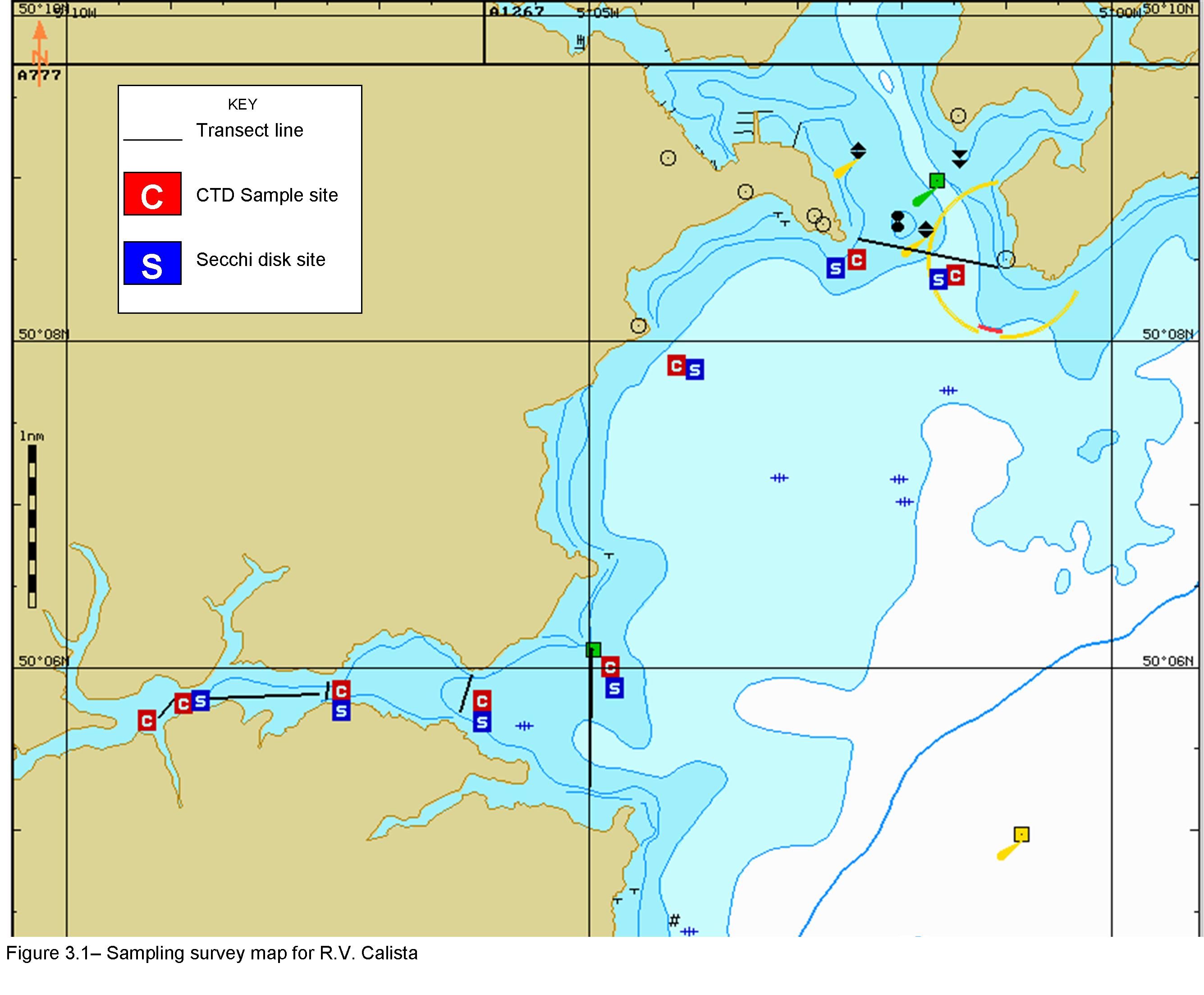
Figure 3.1 - Sampling strategy
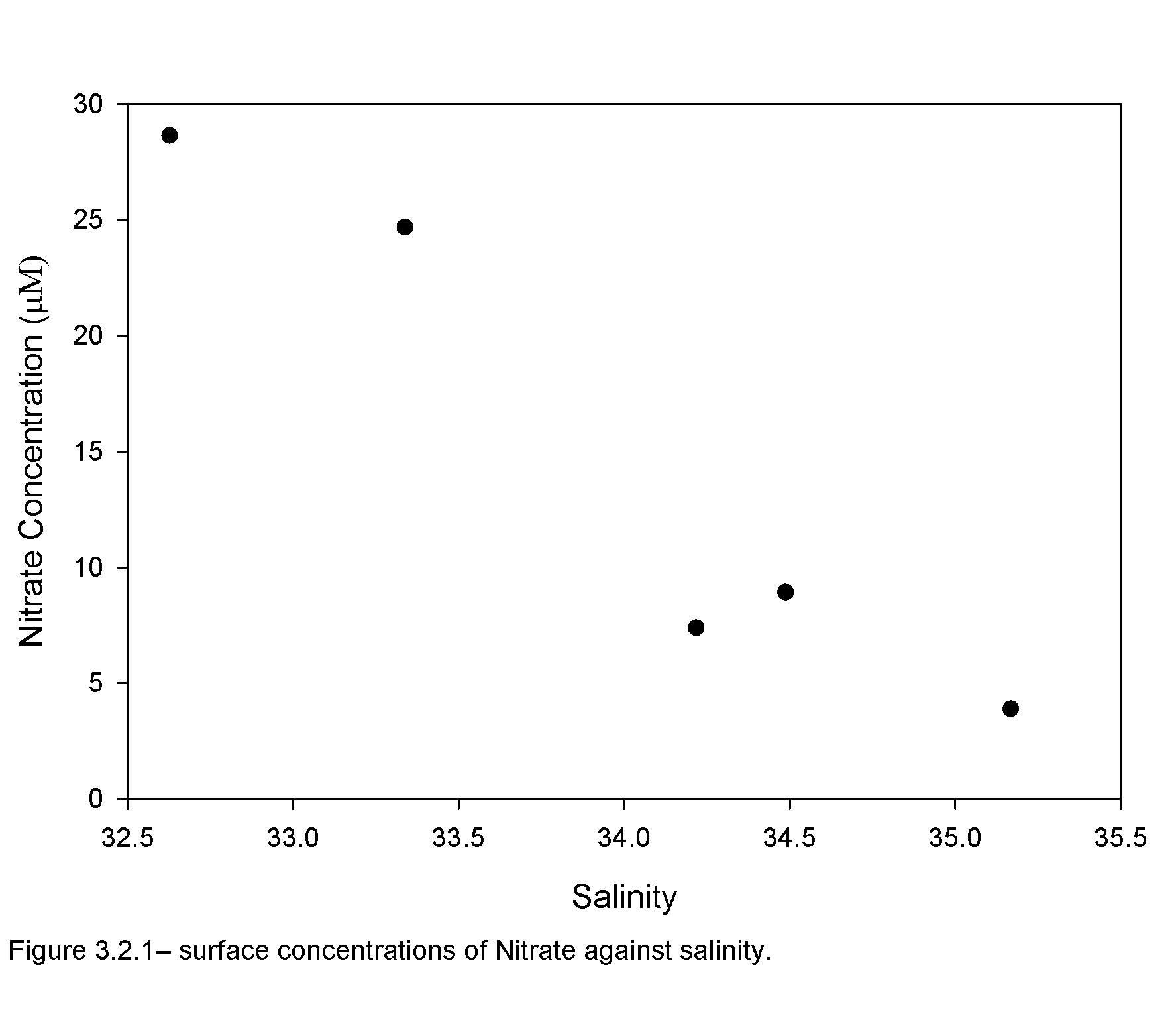
Figure 3.2.1 - Surface nitrate
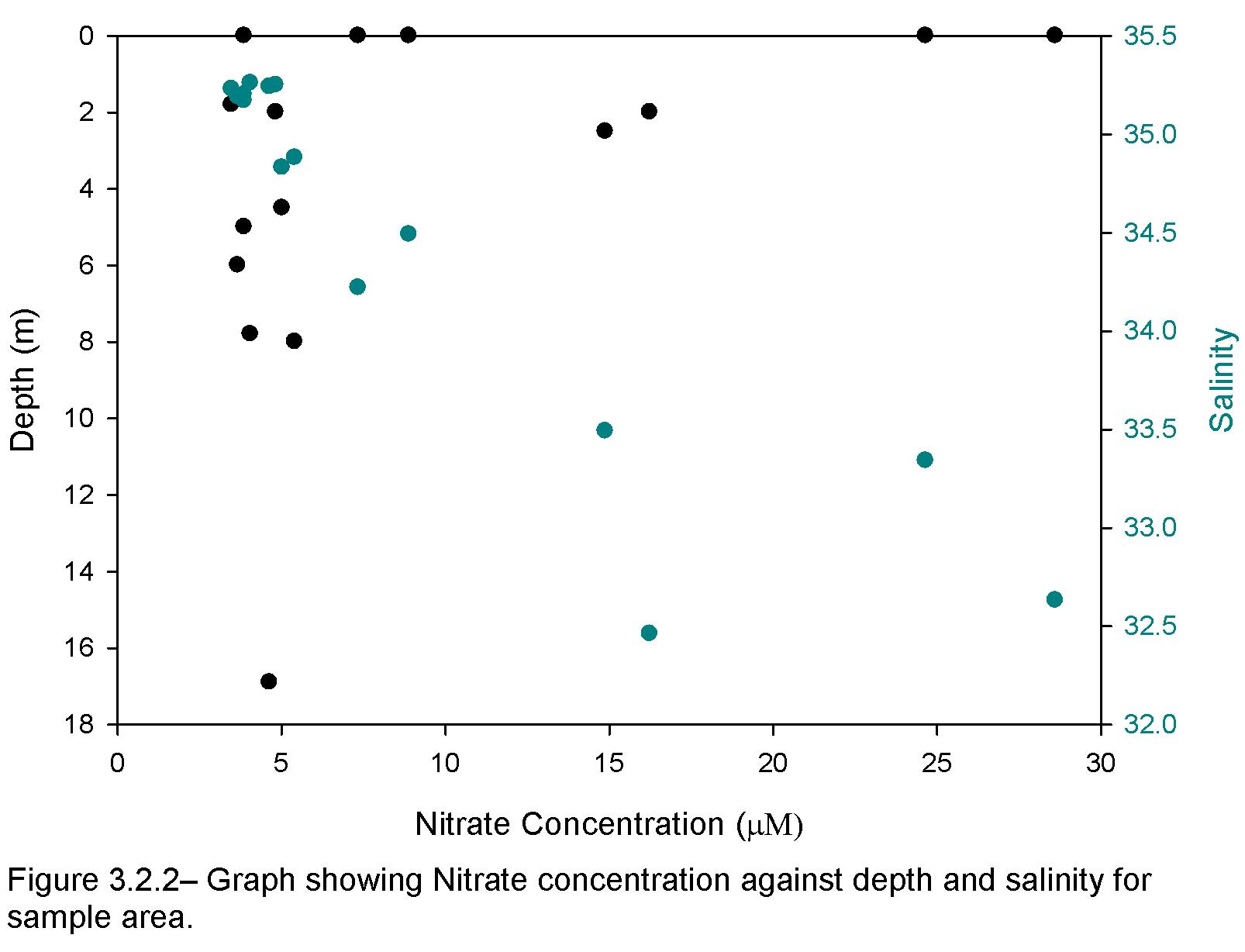
Figure 3.2.2 - Nitrate at depth
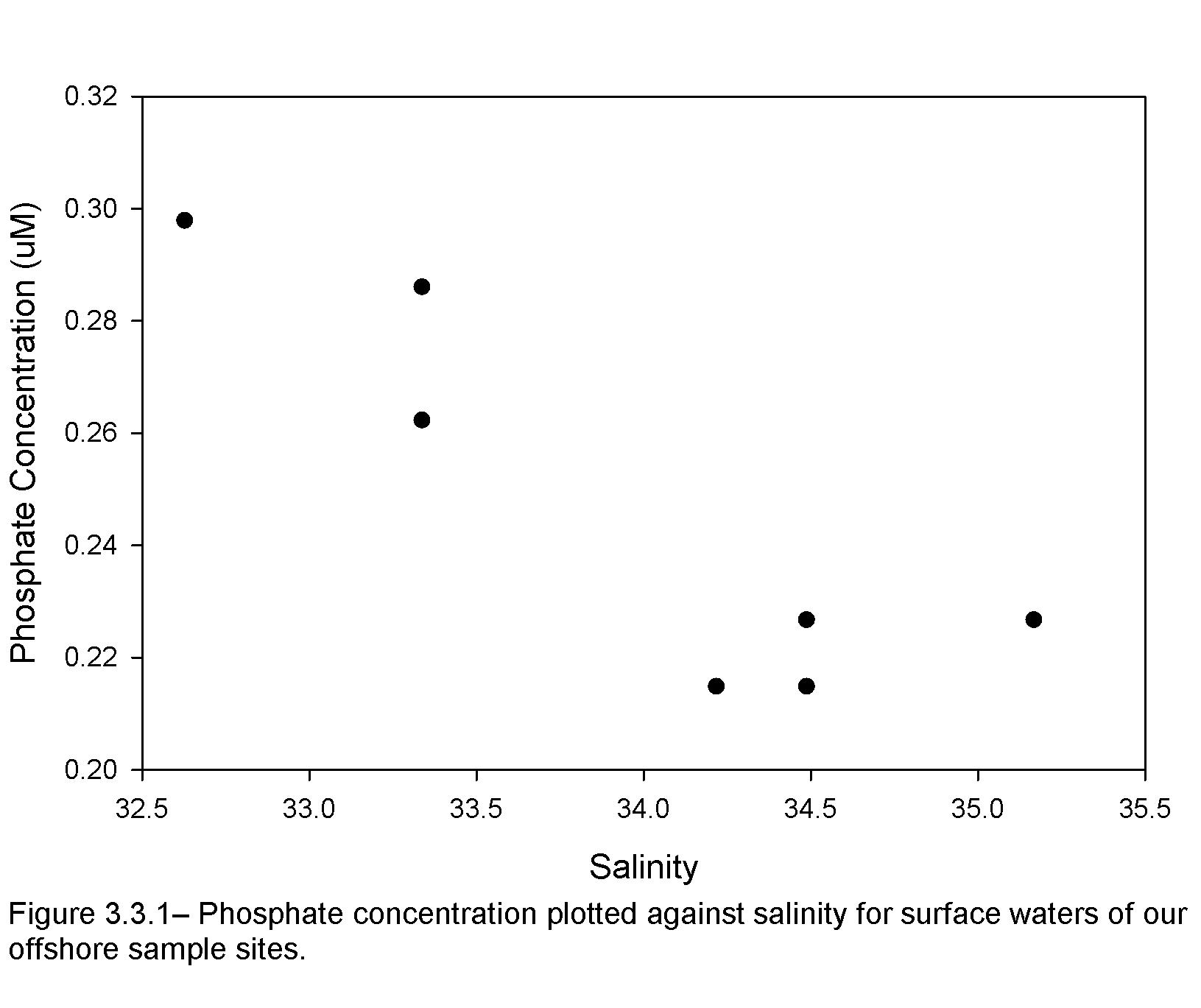
Figure 3.3.1- Surface Phosphate
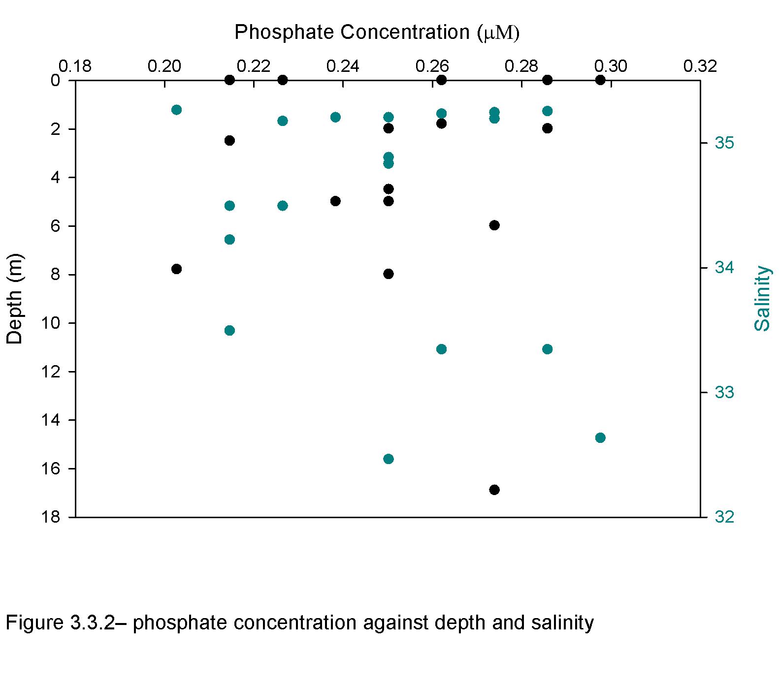
Figure 3.3.2 phosphate at depth
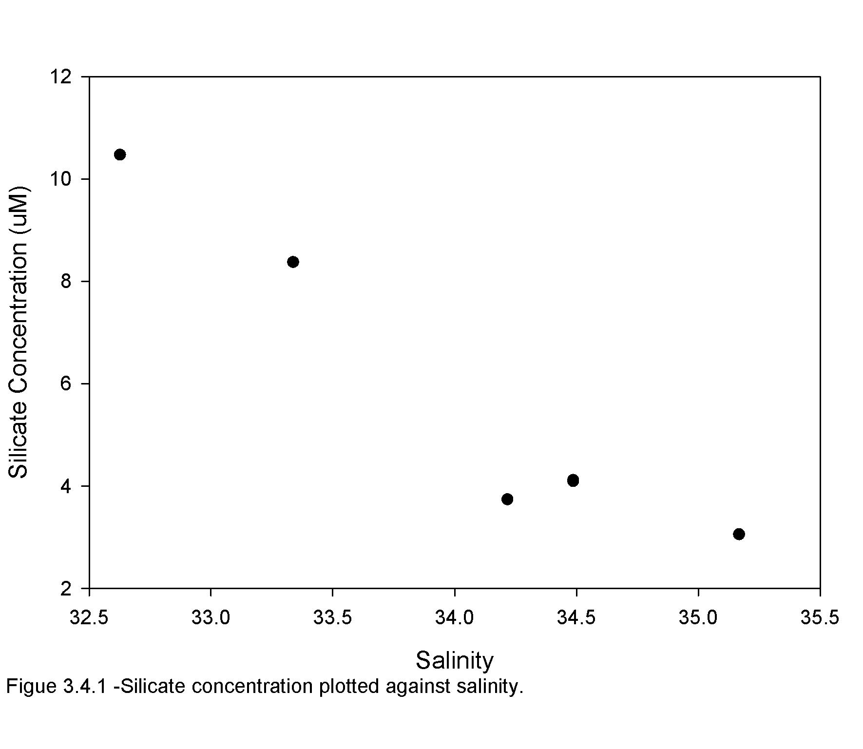
Figure 3.4.1 Surface Silicate
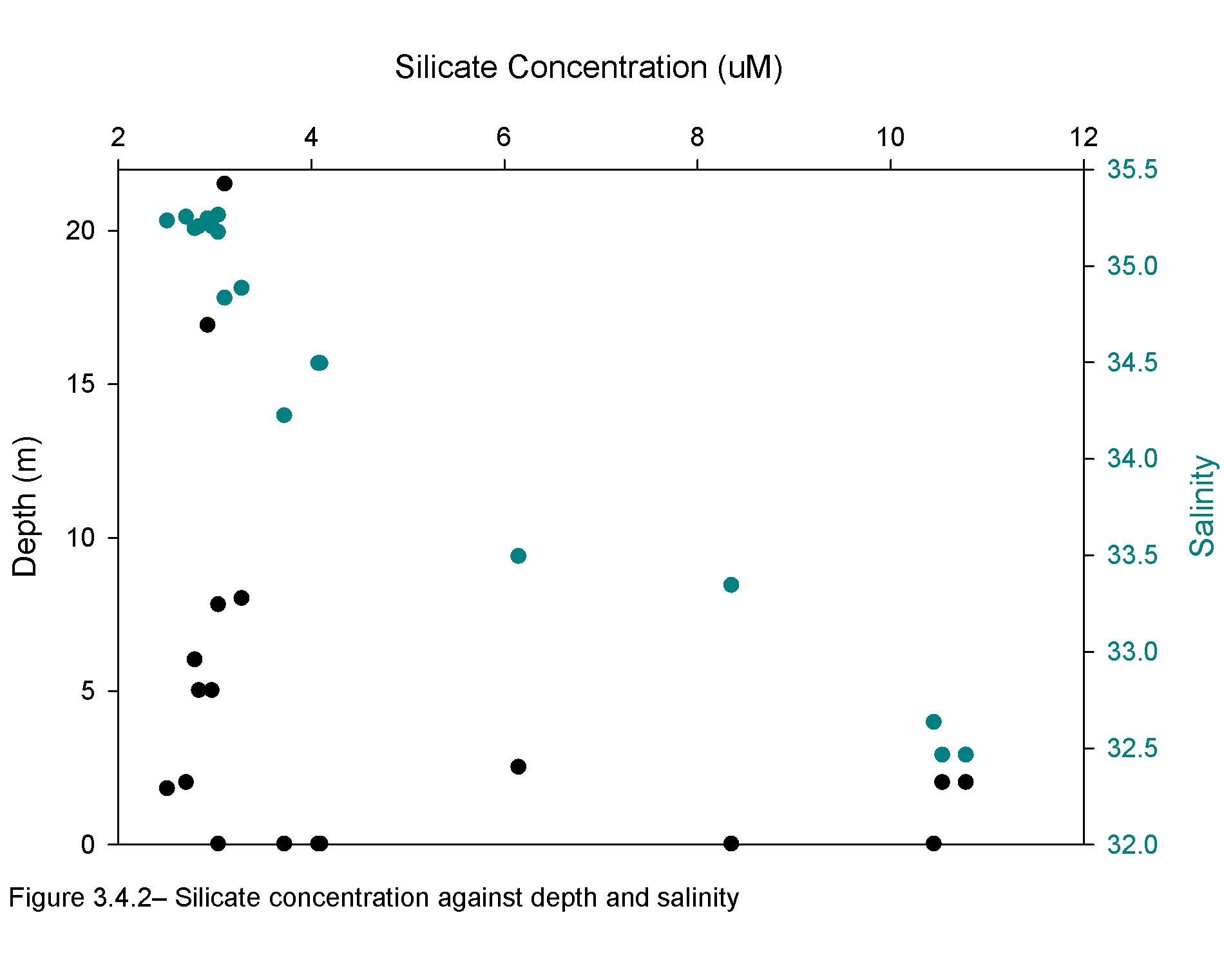
Figure 3.4.2 - Silicate at depth
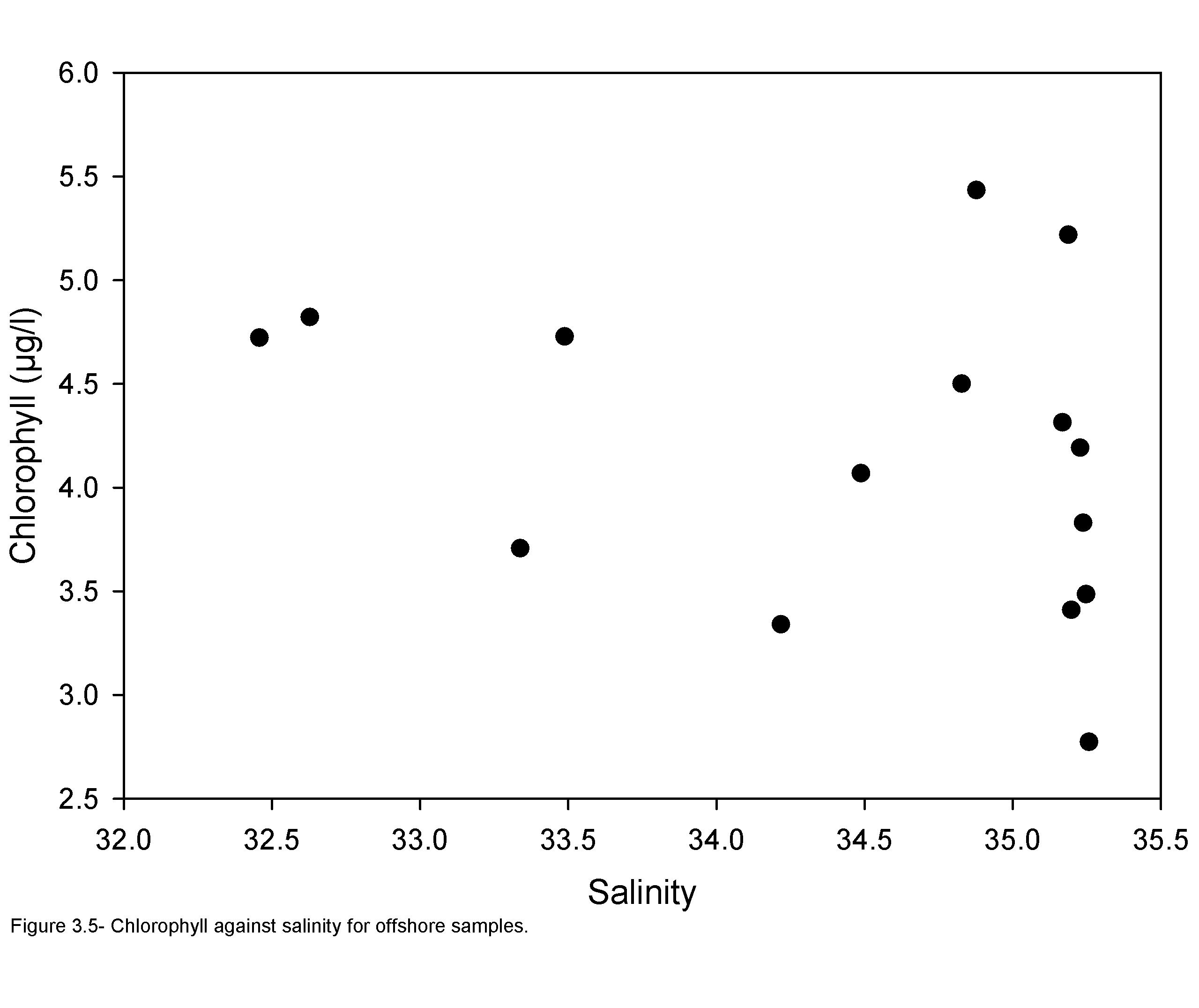
Figure 3.5 - Chlorophyll

Figure 3.9 - Oxygen
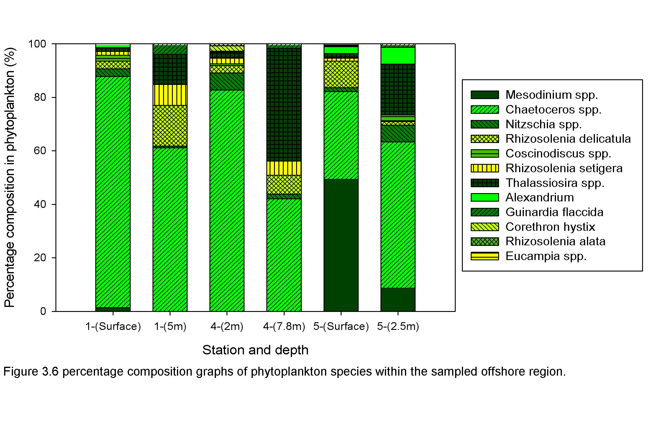
Figure 3.6.1 Phytoplankton
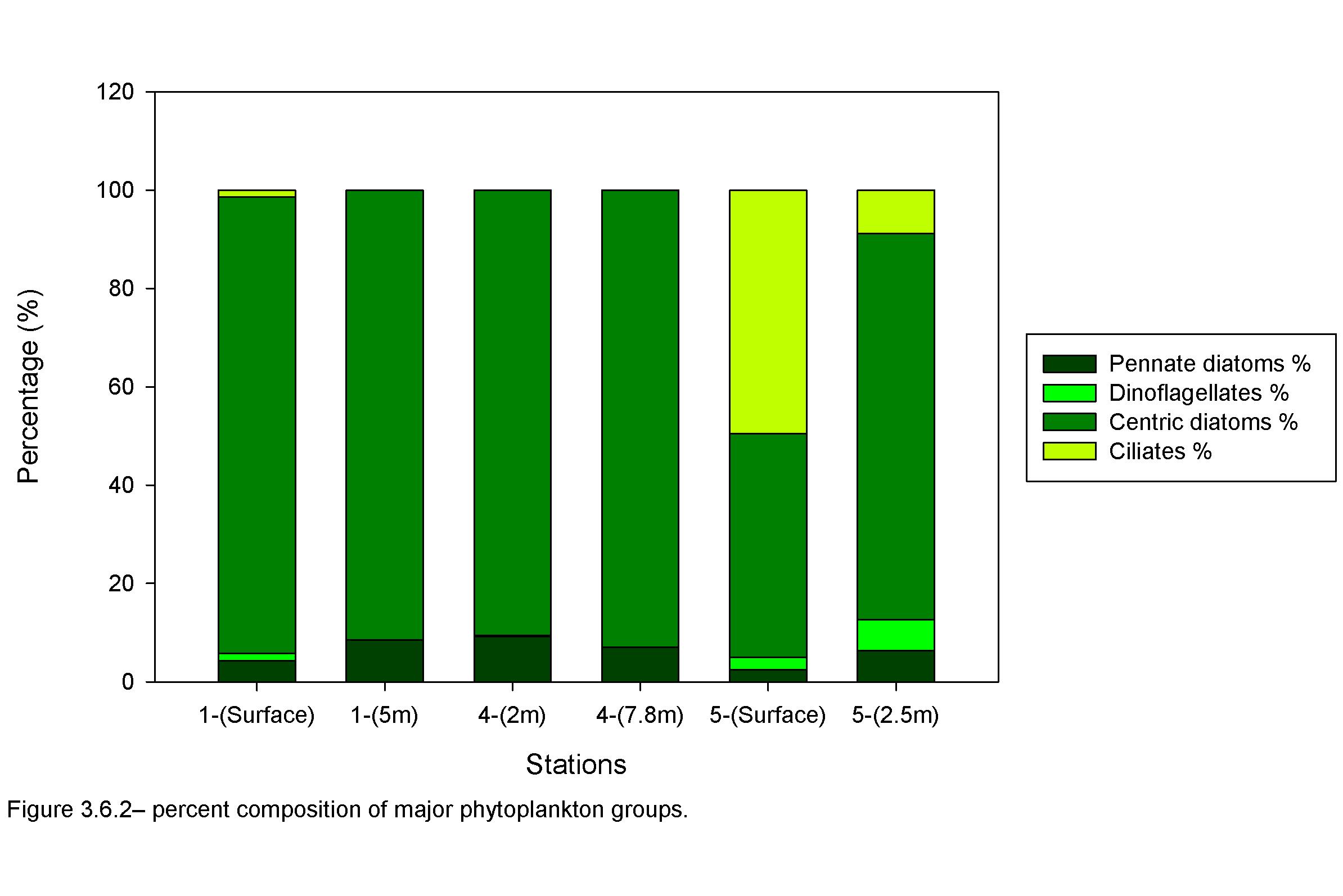
Figure 3.6.2 Phytoplankton groups
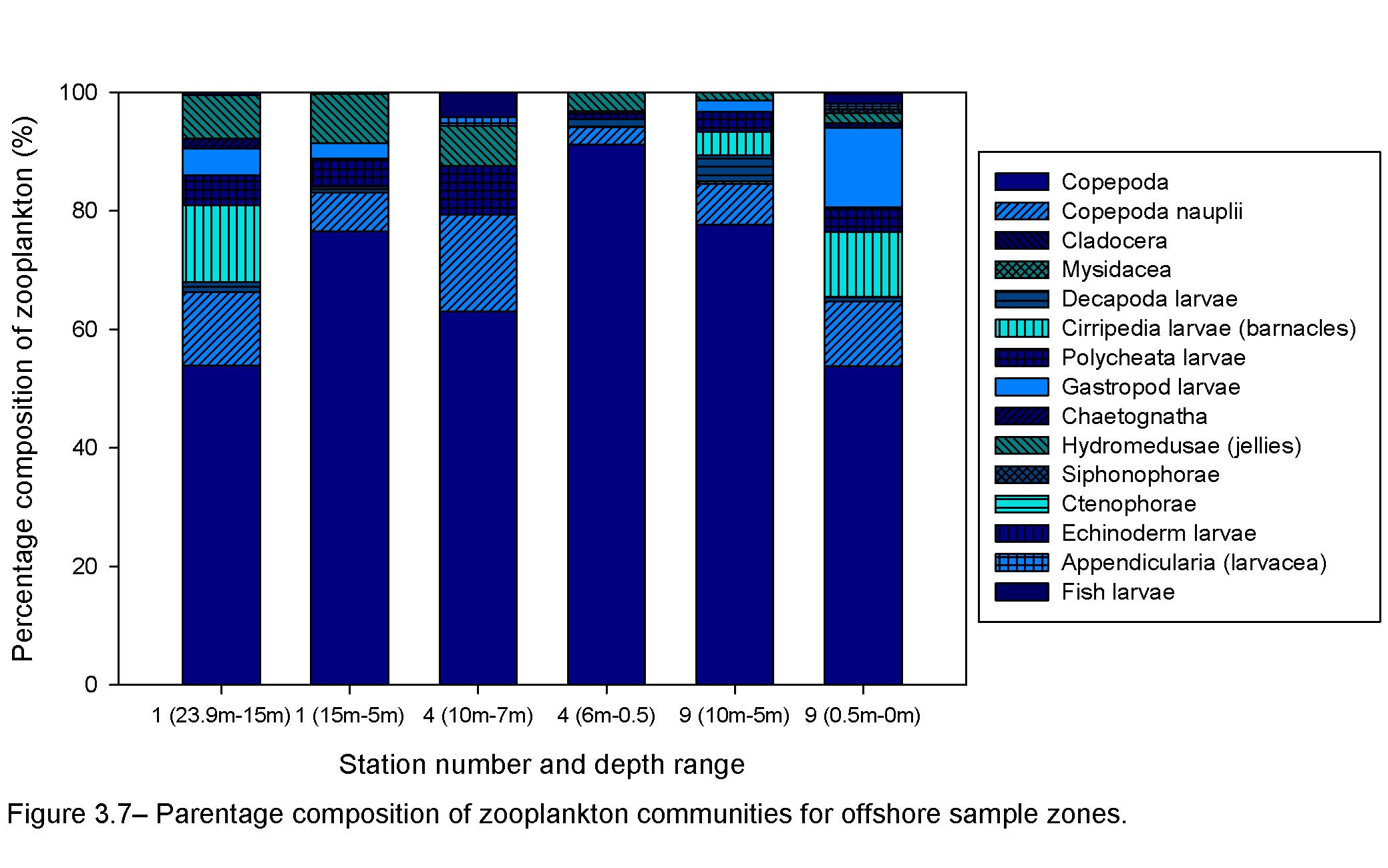
Figure 3.7 - Zooplankton
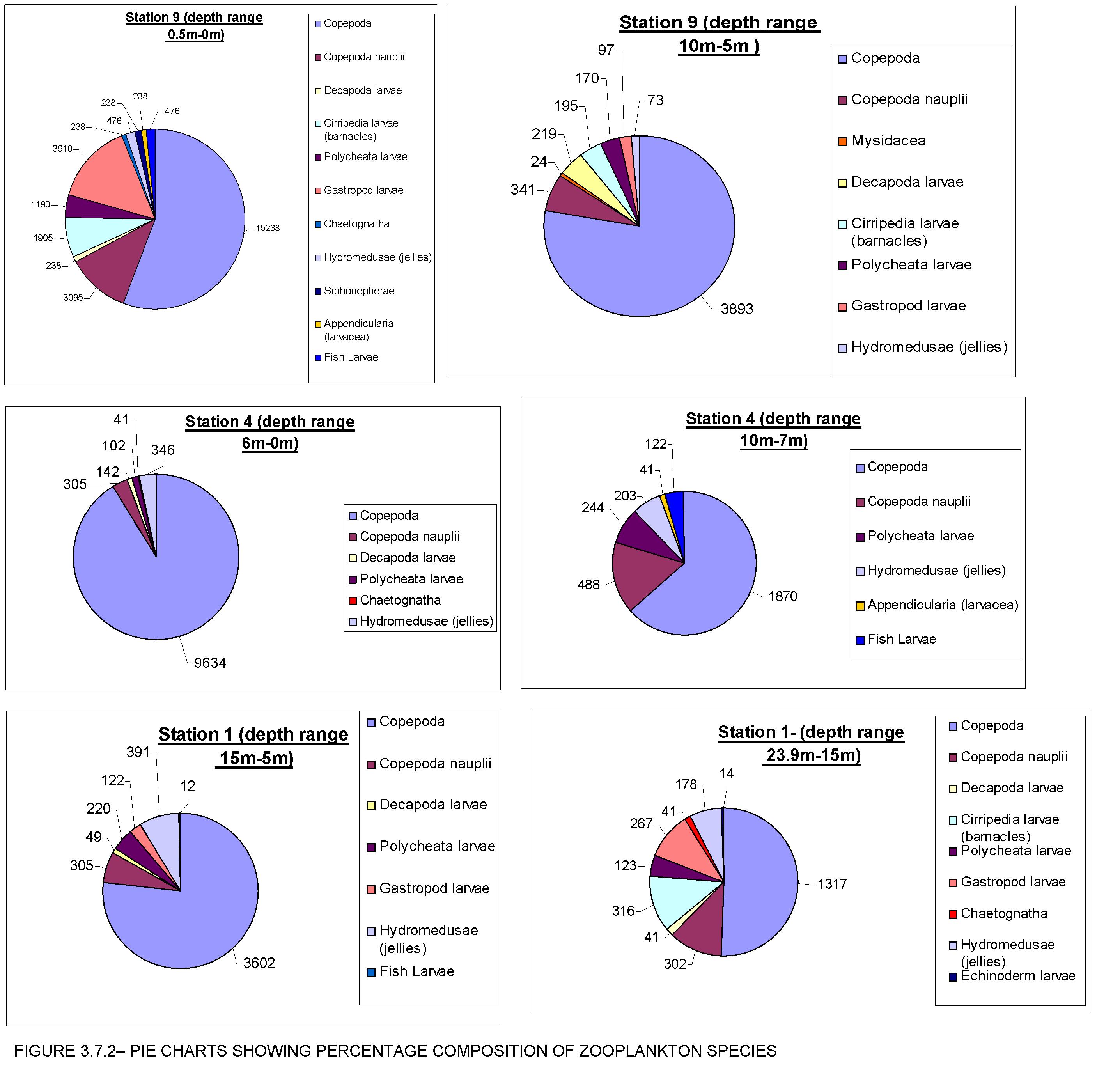
Figure 3.7.2 zooplankton groups
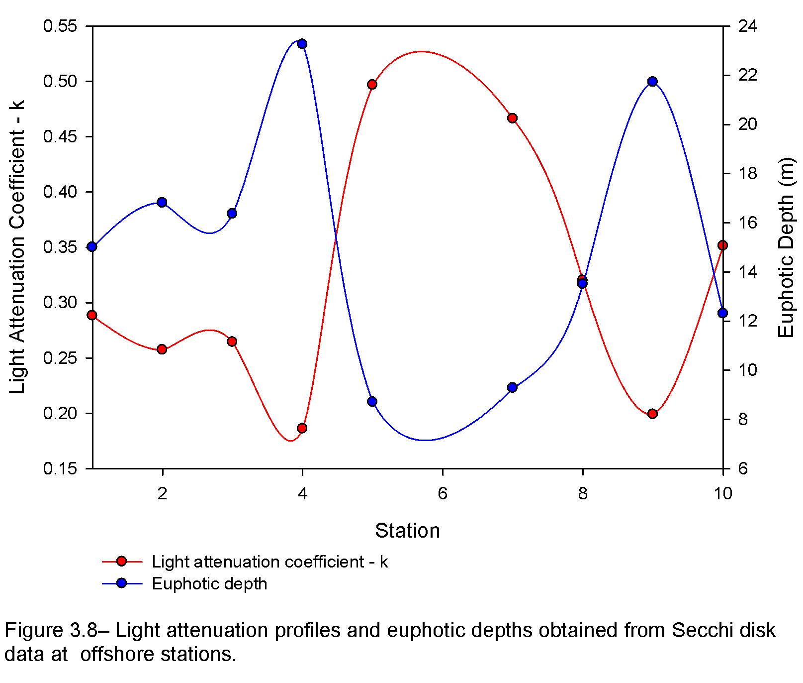
Figure 3.8 - Secchi disk
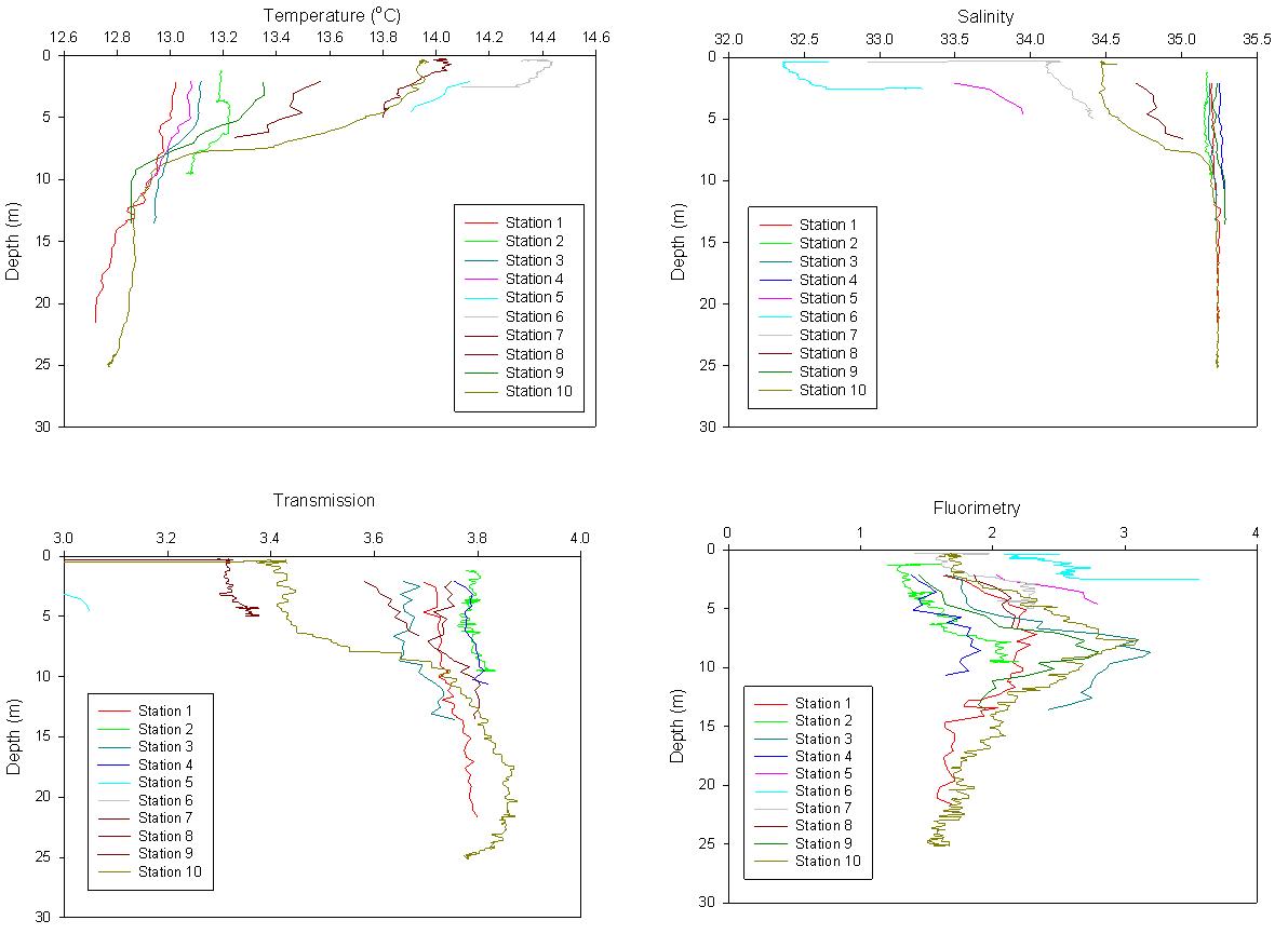
Figure 3.12, Offshore CTD data.
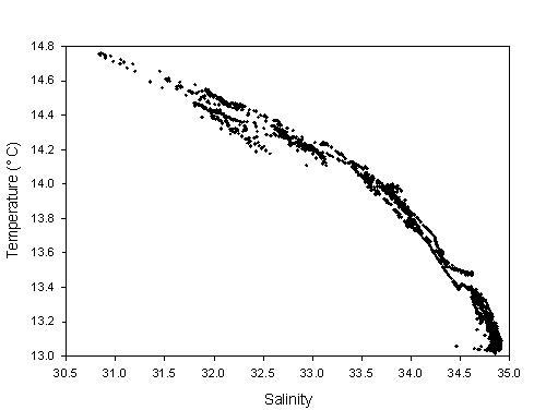
Figure 3.13 - Thermosalinograph
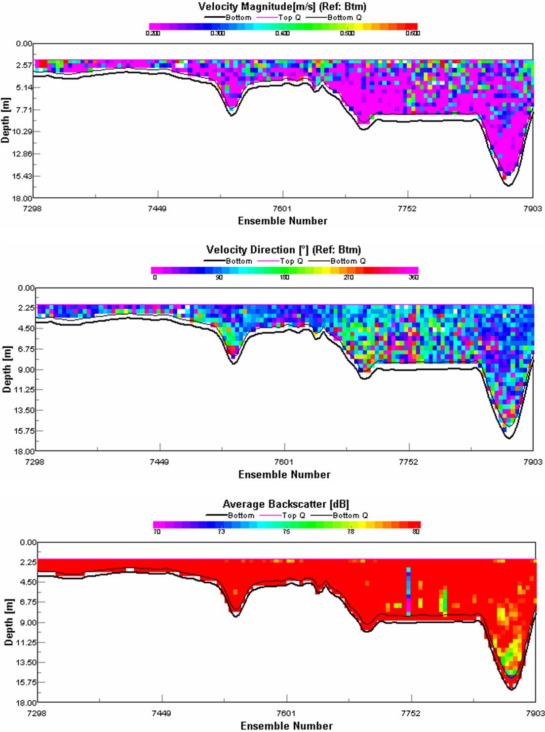
Figure 3.9 - ADCP Station 6
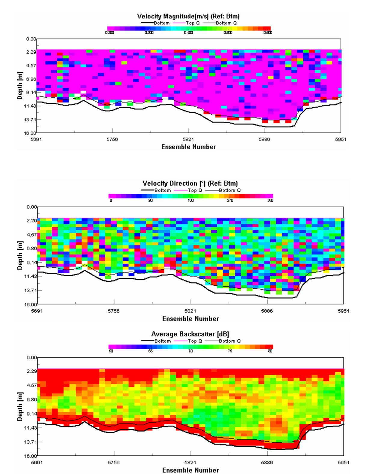
Figure 3.10 - ADCP Station 4
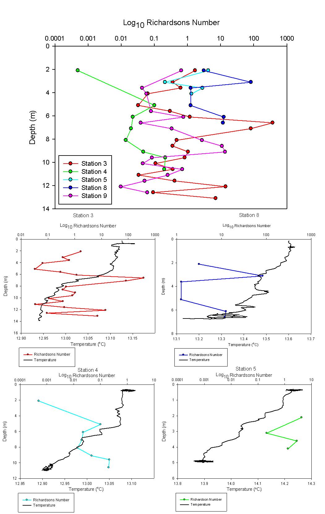
Figure 3.11. Offshore Richardson Numbers
Geophysics - 10/7/07 - Day 8
NAVIGATION
Introduction
The South Cornwall coast between Zone Point, just east of the Fal estuary, and Manacle Point, just south of the Helford estuary, has been selected as a candidate Special Area of Conservation (SAC), recognized for its diverse marine wildlife and beauty by European designation. The drowned river valleys (Rias) of the Fal and Helford support a range of diverse habitats along their length, from sheltered muddy creeks to rocky open coasts, and are recognized as one of the best sites in Europe for their marine life. It is on behalf of Natural England that we were asked to survey and interpret this area with a view to better protecting and conserving the biological and geographical structure of the benthos in this Special Area of Conservation.
Aims
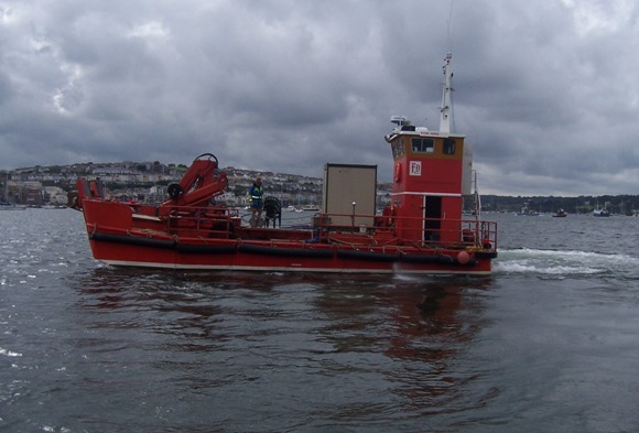
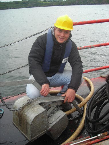
On 10th July 2007 on the R/V Grey Bear we surveyed the topography of the benthos in two regions of the Cornwall coast. For this sidescan sonar was used to try and determine the benthic sediment type and bedforms of the mouth of the Helford Estuary and a stretch of Porthallow Bay. It also necessitated the operation of Van Veen grabs to characterise the benthic fauna at these two locations.
Objectives
To accomplish this aim, we considered the following objectives:
- To use sidescan sonar to survey the two selected regions of the Cornwall coast to build up a picture of the seabed topography.
- To identify and quantify by use of trigonometry the size and frequency of bedforms and to help understand the physical nature of the benthic environment.
- To classify the biology of the benthos through the use of grab samples, at specifically chosen points of interest from the sidescan record.
- To aid in the ongoing survey of the Helford/Fal offshore region for scientific and conservation benefit on behalf of Natural England.
Tides:
|
|
Time (GMT) |
Depth (m) |
Weather: |
|
1st High Water |
0021 |
4.5 |
Overcast for the majority of the day, with an estimated cloud cover of 7/8. The conditions were fairly windy (force 4-5). As the day progressed the temperature increased to approx. 15-16oC and the wind force decreased to 2-3. |
|
1st Low Water |
0706 |
1.6 |
|
|
2nd High Water |
1306 |
4.5 |
|
|
2nd Low Water |
1944 |
1.7 |
Equipment:
|
M.V. Grey Bear - Benthic survey |
| Tow fish- Geoacoustics (model number 159D) |
| Boomer |
| Van veen grab |
| FURUNO LCD sounder (LS-6000) |
| HYDROpro navigation programme |
| Winch system with crane |
| Stacked sieves (sediment grain size analysis) |
| Literature for the identification of marine organisms |
| FURUNO GPS Navigator |
| Geoacoustics sidescan transceiver |
PSO: Dave Watkins
Sampling strategy
Navigation
 Prior to departure
on the M/V Grey Bear two transects were created,
one on the Falmouth Bay
and another in Helford River.
Prior to departure
on the M/V Grey Bear two transects were created,
one on the Falmouth Bay
and another in Helford River.
Two members of the team were collecting data every minute from the start of the transect, recording both latitudinal and longitudinal points but also the time (ATS). Northing’s and Easting’s were also recorded every minute. This enabled us to determine the exact location of any special features recorded on the sidescan sonar.
Sidescan Sonar:
Another two members of the team were viewing the sidescan record. They also had to find any possible location which displayed a particular feature of interest such as ripple bedforms or eelgrass beds in order to determine suitable grab sites.
The rest of the team on decks had the task of spotting any object on the surface such as buoys, boats which could interfere with the sidescan results.
Grab sample locations:
|
Grab Sites |
Latitude |
Longitude |
Time (GMT) |
|
Grab site C1 |
50o06.696N |
005o04.281W |
1415 |
|
Grab site C2 |
50o07.060N |
005 o06.253W |
1425 |
|
Grab site C3 |
50o05.946N |
005 o06.232W |
1515 |
|
Grab site C4 |
50o06.116N |
005 o06.596W |
1536 |
Results
Sidescan sonar:
At station 1 we found evidence of rock formation that created a channel which led to the development of ripple beds. We calculated the average ripple heights at two locations which were 0.19m and 0.24m. We also calculated the average ripple wave length which was 1.40m.The rock formation had an average height of 1.04m with a striking angle of 180o N to S. We also found evidence of anchor drag marks with a calculated depth of 0.56m.
At station 2 in Helford River, the area sampled appears to comprise of both fine and coarse sediments, boundaries between which are not always distinct. To the South-East of the transects there is a possible rock formation indicated by the structures observed by the side scan sonar. We scanned across the expected Eelgrass beds but the sidescan sonar depicts an undefined seafloor. It appears to be a continuation of the finer sediment surrounding it overlain by coarser material. The mottled pattern observed on the scan is reflected in satellite imagery of the station sampled.
Grabs:
Grab site C1
 Due to the
presence of a rocky seafloor the Van Veen grab was incapable of
obtaining a sample at site C1.
Due to the
presence of a rocky seafloor the Van Veen grab was incapable of
obtaining a sample at site C1.
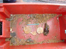
Grab site C2
 The grab had a
large percentage of Maerl, 35% live Maerl, 65% dead Maerl.
We also found two dead scallop shells, two to three coralline algae
species from family Corallinaceae, worms with worm casts, small
bivalves, Cockles (Cerastoderma) and Amphipods.
The sediment was poorly sorted with high angularity. In the grab was
also present a few rocks of small size.
The grab had a
large percentage of Maerl, 35% live Maerl, 65% dead Maerl.
We also found two dead scallop shells, two to three coralline algae
species from family Corallinaceae, worms with worm casts, small
bivalves, Cockles (Cerastoderma) and Amphipods.
The sediment was poorly sorted with high angularity. In the grab was
also present a few rocks of small size.
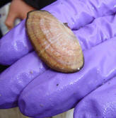
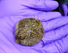
Grab site C3
 Grab site C3
brought up some Sea potatoes (Echinocardium cordatum), common
Dogwhelks (Nucella lapillus), tube casts from worms, a sunset
shell (the dark rim around shell is most likely from stress, such as
existing in salinities lower than normal), amphipods, isopods and
cockles (Cerastoderma).
The sediment was fine and well sorted with a uniform grain size but with
a unknown angularity.
Grab site C3
brought up some Sea potatoes (Echinocardium cordatum), common
Dogwhelks (Nucella lapillus), tube casts from worms, a sunset
shell (the dark rim around shell is most likely from stress, such as
existing in salinities lower than normal), amphipods, isopods and
cockles (Cerastoderma).
The sediment was fine and well sorted with a uniform grain size but with
a unknown angularity.
Grab site C4
The sample from grab site C4 had some small crabs, polychaete worms, sea squirts (Ascidian), amphipods and Eelgrass. The sediment was moderately sorted; the type of mud was muddy sediment.
Discussion Grey Bear
In Falmouth Bay, between Rosemullion
Head and offshore of Maenporth, rocks and coarse sediments dominate the
seafloor. The formations of the rocks created channels down which water
is funneled to form ripple beds. The ripple beds are uniform in height
and wavelength around the rock formations, however, as depth increases
with distance from these, larger ripples were observed. Anchor drag
marks are also observed, caused by the high level of industrial activity
in the Fal Estuary. Near to the shore an anomaly appeared which is thought to be an
Eelgrass bed. However, because of the proximity to land the scattered
effect on the scan suggests it could also be shingle.
coarse sediments dominate the
seafloor. The formations of the rocks created channels down which water
is funneled to form ripple beds. The ripple beds are uniform in height
and wavelength around the rock formations, however, as depth increases
with distance from these, larger ripples were observed. Anchor drag
marks are also observed, caused by the high level of industrial activity
in the Fal Estuary. Near to the shore an anomaly appeared which is thought to be an
Eelgrass bed. However, because of the proximity to land the scattered
effect on the scan suggests it could also be shingle.
Grabs were taken at a number of sites to verify the findings of the sonar scans. At C2 the Maerl bed dominated the benthos, and restricted the presence of species found elsewhere. The substrate at C3 is well sorted and fine grained due to the low flow velocity in this area. Species diversity was greater here than at other sites due to the presence of selective particle feeders that predate upon meiofauna. The Eelgrass bed was sampled at site C4, however, only a limited amount of Eelgrass was recovered. This suggests that the grab only sampled the edge of the bed. The moderately sorted sediments at this location led to the presence of sea squirts that require a hard substrate habitat. The muddy sediments here are ideal for polychaete communities and the Eelgrass provides a sheltered environment for juvenile crustaceans.
Figure 4.1 - Sea floor type boundaries
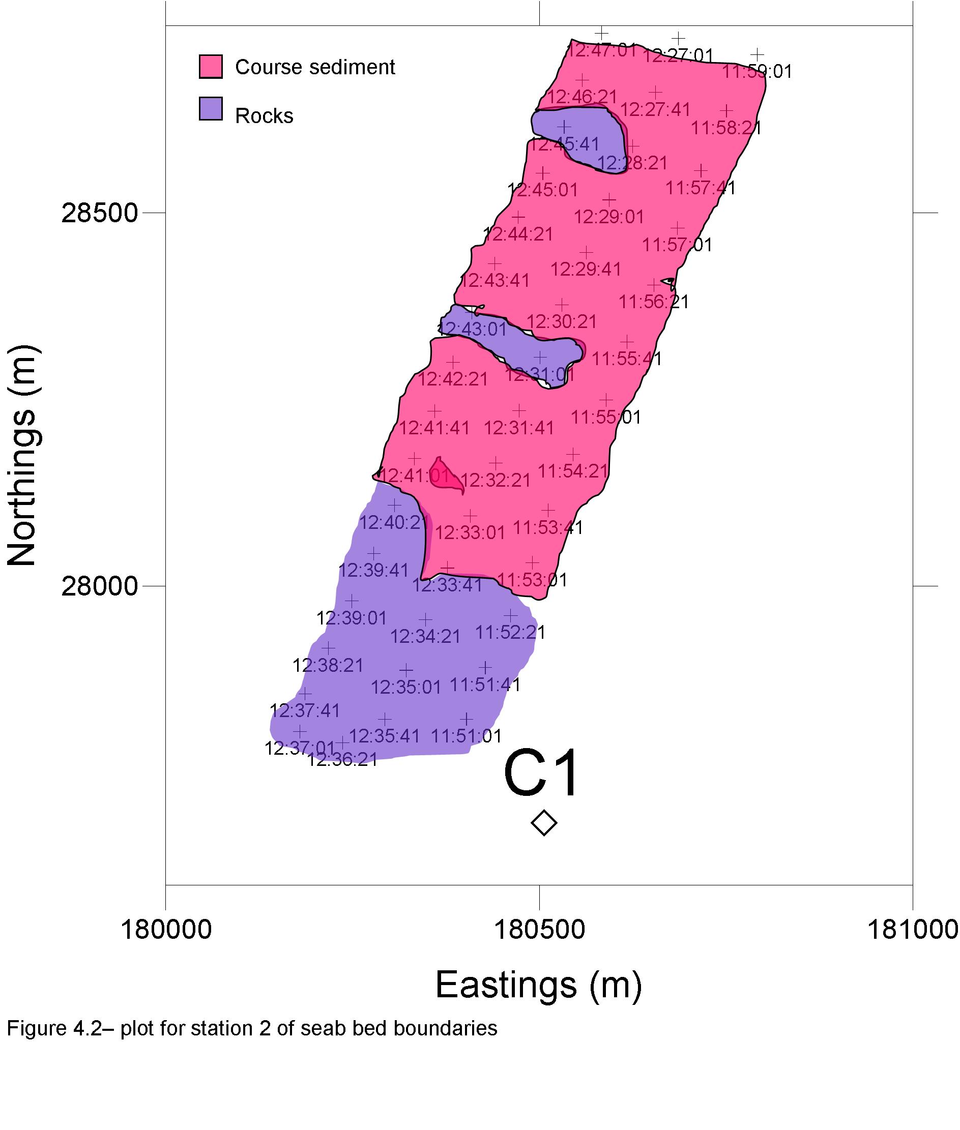
Figure 4.1 - Sea floor type boundaries
NAVIGATION
Parsons T. R.
Maita Y. and Lalli C. (1984) “ A manual of chemical and biological
methods for seawater analysis” 173 p. Pergamon.
Grasshoff, K., K. Kremling, and M. Ehrhardt. (1999). Methods of seawater
analysis. 3rd ed. Wiley-VCH
Johnson K. and Petty R.L.(1983) “Determination of nitrate and nitrite
in seawater by flow injection analysis”. Limnology and Oceanography
28 1260-1266.
Parsons. T. R., Maiti. Y., Lalli. C. M. (1984) A manual of chemical and biological methods for seawater analysis. Pergamon Press. Oxford. 173pp.
Grasshoff, K., Kremling, K., and Ehrhardt, M. (1999). Methods of seawater analysis. 3rd ed.
Wiley, VCH., Johnson K. and Petty R.L.(1983) “Determination of nitrate and nitrite in seawater by flow injection analysis”. Limnology and Oceanography 28 1260-1266.
