|
|
Falmouth Field Trip '07 |
|


Contents
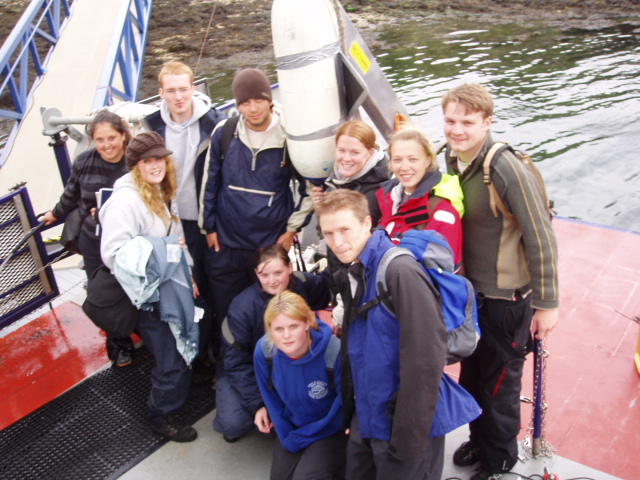
Group 2 and the rare blue finned white shark!
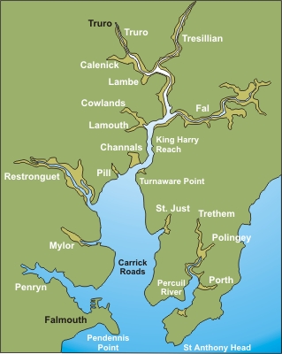
Map of the Falmouth Estuary
The Fal Estuary has a very common shape for the south west of England; it is one of many “drowned river valley” estuaries (Farnham, 1985), which are also known as rias. These are formed because of the sea level changes that have occurred since the last ice age 18,000 years ago. Rising sea level causes nearby river valleys to flood with sea water. As the rates of sedimentation cannot keep up with the water flow sediments are washed away too quickly. The estuary retains its v-shaped basin with extensive sand/mud flats in the inter-tidal zone (Hawkins 2006). Typically rias have many small rivers branching off a narrow long estuary (Fischer et. al. 1979); this is seen in the Fal for example Restronguet Creek and Penryn River. The Fal has a deep channel with a depth of 30m (which prevents the need for dredging) and the wide shallow banks on each side are 4-5m in depth. The Fal is a fully saline body of water (Farnham & Bishop 1985), it has riverine inputs at the head, but the exchange of water is so rapid that the fresh water gets washed out.
The Fal has been designated a Special Area of Conservation (SAC) by Natural England, protecting rare and threatened fauna and flora both on shore and in the estuary. They support a range of habitats from sheltered muddy creeks to rocky open coasts (Natural England 2006), for example centuries old shell fisheries and extensive maerl beds. Maerl is a calcareous seaweed which is extracted for the use of lime in farming. New regulations mean that only dead maerl is extracted, however despite this measure there are few maerl beds left in the country.
Mining was originally the predominant industry of the Fal where Arsenic, Tungsten, Uranium, Silver and China Clay were among the minerals mined. In 1991 the mines were closed, however drainage of metals into the estuary still occur. The most recent incident was in Restronguet Creek in February 1992.
The Fal is one of the most metal polluted estuaries in the UK due to dredging and the marine industry, for example TBT anti-fouling. TBT anti-fouling causes raised ammonia levels, is toxic to fish and can lead to imposex in dog whelks, mussels and oysters.
The Fal estuary is therefore an interesting place to study, with both anthropogenic and natural impacts on the biological communities within the estuary. The aim of this two week survey is to investigate the chemical, physical, geophysical and biological aspects of the Fal estuary.
Date: 03/07/07
Tides: HW 4.9m 07.02GMT, LW 1.2m 13.28GMT, HW 5.2m 19.11GMT
Boat: MV Grey Bear
PSO: Sam Drawbridge
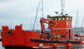
Fig 1. MV Grey Bear
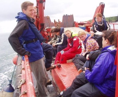
Fig 2. The Team
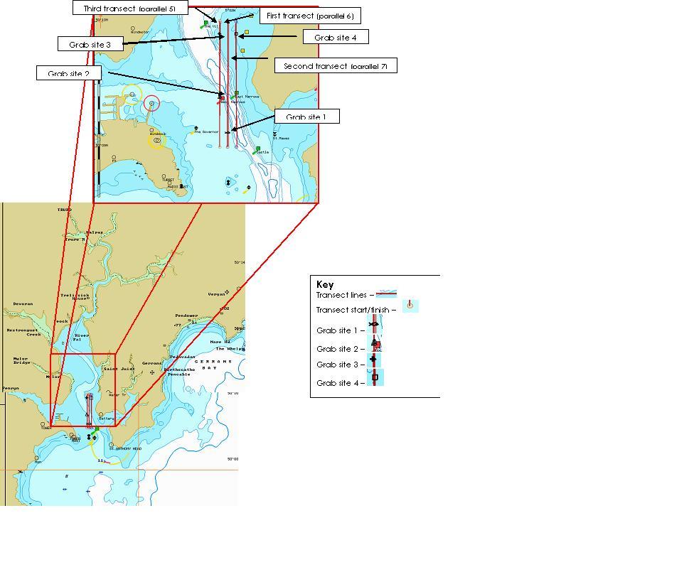
Fig3. Map showing the transects for the geophysics survey in Carrick Roads
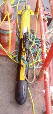
Fig 4. Side Scan Sonar
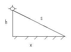
Fig 5. A graphical representation of the sweep of the side scan sonar used for the seabed depth equation.
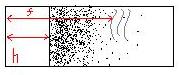
Fig 6. Graphical representation of the side scan trace, showing f, the distance from the side scan to the feature, and h, which is water depth.
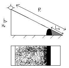
Fig 7. Graphical representation used to work out the height of a target.
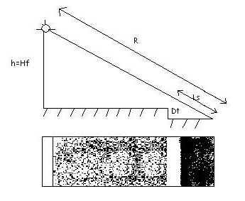
Fig 8. Graphical representation used to work out the depth of a target
![]()
Fig 9. Surfer plot showing the transects and the sites of the grabs.
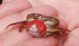
Fig 10. A pregnant velvet swimming crab (scientific name)
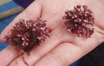
Fig 11. Maerl
The aim of this survey was to investigate the topography of the Fal estuary and the benthic composition of the seabed, including the sediment and the biological composition.
The Fal estuary and surrounding area is a site of Special Area of Conservation. It is one of the largest natural harbours in the world and is a unique ecosystem. It is also used for aquaculture, including oyster fishing, and recreational boating. As such Natural England is interested in maintaining an up to date record of the area in order to aid conservation, without preventing anthropogenic activity.
As part of this, our brief was to collect and analyse data on the area using the MV Grey Bear (Figure 1) and side scan sonar and grab equipment, which can then be fed back and will be useful to Natural England in their conservation of the area.
Allocated Jobs
-PSO (Principal Scientific Officer) – Sam Drawbridge
-Deputy PSO – Lorna Wrigley
-Feature Data Loggers – Jonny Bliss & Emma Rathbone
-Positional Data Loggers – Josh Georgiou & Alex Lord
-Spotters – Molly Steele, Christina Wood & Catherine Chatwin
-Navigator – Chris Sturdy
-Figure 2 shows the team!
Survey
The PSO chose three transects to examine the seabed using the side scan sonar. They were spaced 100m apart and each transect measured 2km in length. Unfortunately, our geophysical survey was limited to Carrick Roads due to the tide times and poor weather conditions. From the printouts using the side scan sonar (Figure 4), we selected four seemingly contrasting areas of interest to take samples using the Van Veen grab.
Side scan sonar was used to create a picture of the sea floor over various transects at Carrick Roads. The different returns were used to determine different features. Grab samples were used to investigate interesting features from the side scan printout, and also provide information on the marine benthos present at the different sites.
Surfer plot was used to produce a route map of the MV Grey Bear. The map was segregated by boundaries of the different acoustic returns. Also plotted were the grab sites which gave insight into the marine benthos.
A Scientific poster was created to summarise the findings from the geophysics practical.
Side scan sonar and Surfer Plot
The first objective back in the lab was to arrange the 3 side scan transect printouts so the features could be identified and matched up along the three sets of data. From this a surfer plot was created using position (Northings and Eastings) and time, which showed a transect route on a geographical scale. From the side scan printouts we identified significant boundaries between areas. We then picked points to encompass the features and enable them to be drawn onto the surfer plot. The distance between the centre of the plot and the points was measured, enabling us to use equations to determine seabed depth and range correction;
| Seabed Depth (Fig 5) | Range Correction (Fig 6) |
|
h (cm) = h(m) X (cm) x (m)
|
F (cm) = F (m) X (cm) X (m)
|
|
h (cm) x 75 = h (m) X (cm)
|
F (cm) x 75 = F (m) X (cm)
|
| X = √S2 – h2 | |
| Height of Target (Fig 7) | Depth of Target (Fig 8) |
| HT=(Ls x Hf)/R | DT=(Ls x Hf)/(R-Ls) |
Where h = height of fish above seabed
X = the distance from the centre of the printout to the edge
F = the distance from the centre of the printout to the point
S = the actual distance from the fish to the point
We could then use the distances obtained to create a diagram demonstrating the sediment type based on strength of reflection (Figure 9). The rest of the afternoon was spent creating a poster to display our results. Grab samples were analysed and biota photographed was identified as far as possible. Significant findings are included on the poster. A graph was produced to show topography with depth verses distance determined using the same method as above with various points taken along the transect.
Grab Samples
On analysing the side scan sonar traces four different acoustic returns were found. These were interpreted as kelp, soft/silt sediment, coarse sediment and bed rock. An unknown feature, approximately 7 by 15 meters was found at time 11:59:20 GMT.
Grab site A
Location: 50o 09.1 N, 5o 02.0 W
Time: 1249 GMT
Weather: Windy and raining
Summary of findings:
Sediment type – a fairly poorly sorted mixture of fine, grey/brown sand, several rocks and small fragments of broken up shells, overall creating a quite coarse sediment that appears to be bioclastic.
Estimated composition – shell fragments (70%), sand (20%)
Biota
-No obvious live organisms except sparse miniature seaweed (Dilsea carnosa or Calliblepharis ciliate/red fringe weed)
-Shells found but all dead
Grab site B
Location: 50o 09.4 N, 5o 02.1 W
Time: 1310 GMT
Weather: Windy and raining
Summary of findings:
Sediment type – mostly dead, slightly broken up maerl (80%), low proportion of live maerl, some sand, lots of shells and shell fragments (15%), some alive, a few rocks – metamorphic slate typical of the area.
Estimated composition – dead maerl (80%), shells and shell fragments (15%), little sand or rocks
Biota
-Grey topshell
-A species of clam
Grab site C
Location: 50o 08.9 N, 5o 02.1 W
Time: 1328 GMT
Weather: Spitting, 7/8 cloud cover
Summary of findings:
Sediment type – very fine, some stones, lots of live maerl. Some dead maerl in smaller fragments, some clam fragments. Sediment was sieved with 2 and 1 mm mesh sieves.
Estimated composition – live maerl (50-60%), mud/sludge (30%), seaweed remaining fraction
Biota
-Pregnant crab – velvet swimming crab Necara pubis (Figure 10)
-Maerl (alive) – red and purple (Figure 11)
-Polychaete
-Lugworm – Arenicola marina
-Brown seaweed Chondrus crispus
-Red seaweed – Ceramiun sp.
Grab site D
Location: 50o 09.9 N, 5o 01.9 W
Time: 1315 GMT
Weather: 7/8 cloud cover, dry but quite breezy
Summary of findings:
Sediment type – very fine grey mud and lot of maerl, almost all alive
Estimated composition – maerl (60%), fine mud 30-40%
Biota
-Long clawed lobster
-Lots of brown seaweed
-Clam with tiny barnacles (about 3 mm)
-Brittle star
-Amphipod
-Swimming pea crab
-Red seaweed – Ceramium sp.
The grab samples found differences in sediment composition and the organisms found there. The main sediment types were shell fragments (Site A), maerl (Site B, C) and fine mud found upstream at Site D. Site D also had the most interesting range of organisms which included Necara pubis and Arenicola marina. Other biota found included polychaetes (site B) and the seaweed Chondrus crispus (site C). The combined transects of the side scan sonar also revealed an apparent area of bedrock running approximately perpendicular. However the side scan sonar print out did prove difficult to interpret in places. This was mostly due to the inconsistent level of noise, which was mainly caused by the boats propeller. Furthermore the side scan sonar print out also showed some very interesting seafloor topography depicted on the poster.
Date: 06/07/07
Tides: LW 1.1m 03.15GMT, HW 4.7m 09.09GMT, LW 1.3m 15.31GMT, HW 5.0m 21.20GMT
Boats: RV Bill Conway and RIB Ocean Adventure
PSO: Jonny Bliss (RIB Ocean Adventure) and Cathrine Chatwin (RV Bill Conway)
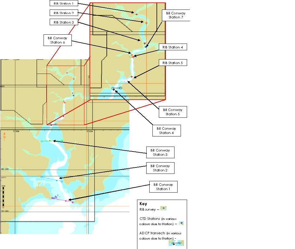
Figure 1. Map showing the survey sites of both RIB Ocean Adventure and RV Bill Conway.
|
Fig 2. RIB Ocean Adventure |
Fig 3. RV Bill Conway
|
|
Fig 4. The CTD being deployed |
Fig 5. Samples taken from the Niskin bottle
|
|
Fig 6. YSI probe used on the RIB |
Fig 7. Sampling on board the RIB
|
|
Fig 8. Plankton trawl and CTD on board the Bill Conway |
Fig 9. Oxygen sampling
|
|
Fig 10. Plankton ID in the lab
|
Fig 11. Nutrient analysis
|
|
Fig 12. Nutrient analysis
|
|
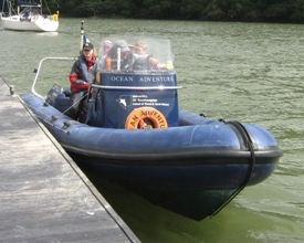
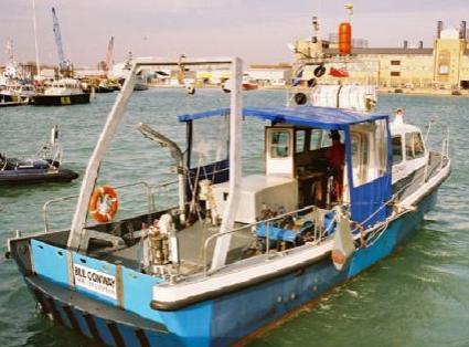
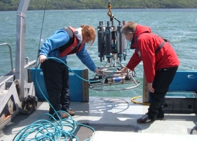
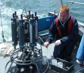
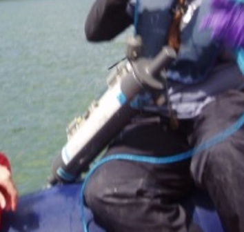
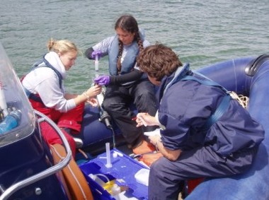
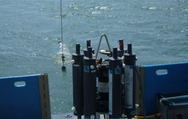
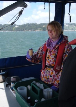
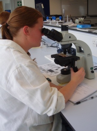
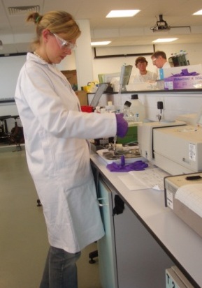
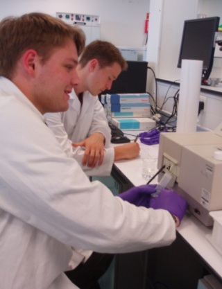
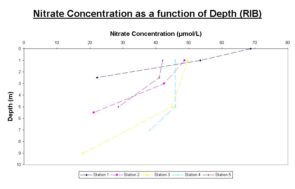
Fig 13 |

Fig 14 |
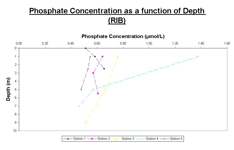
Fig 15 |
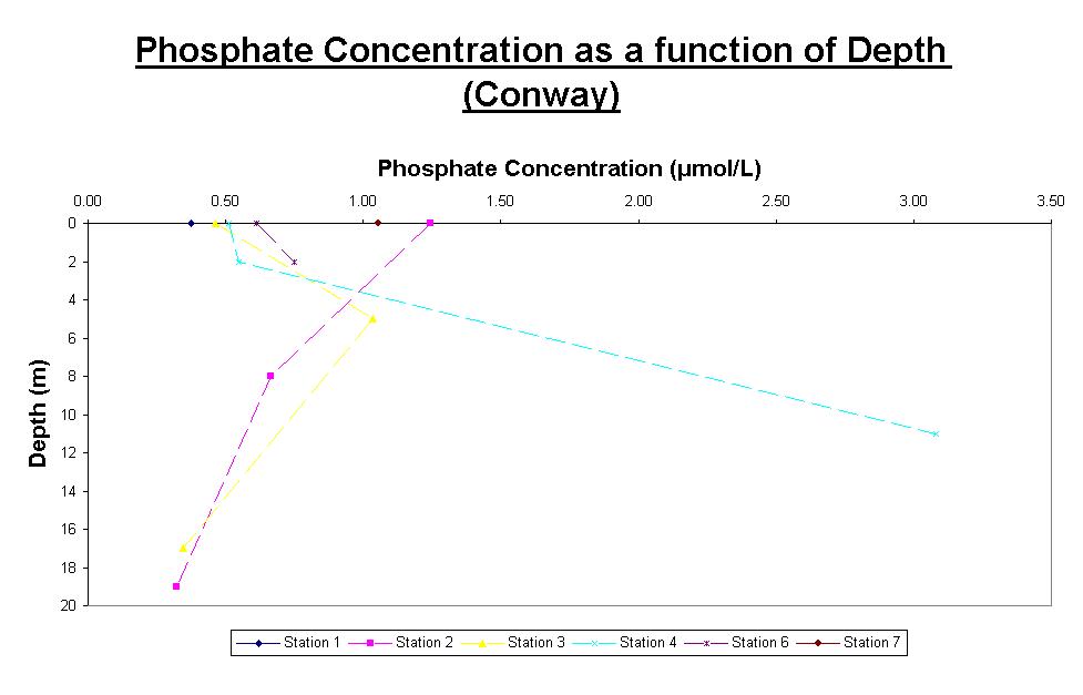
Fig 16 |
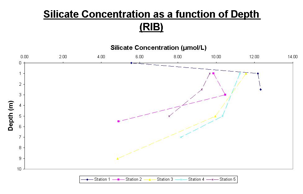
Fig 17 |
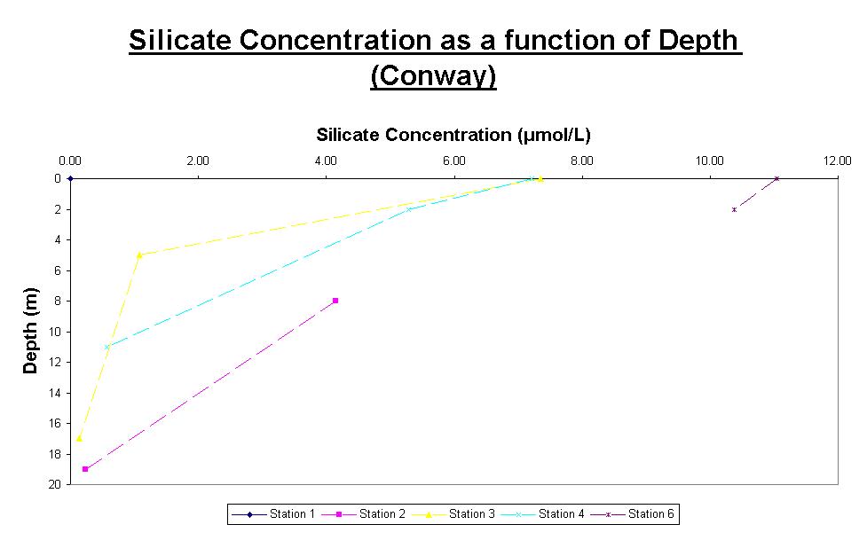
Fig 18 |
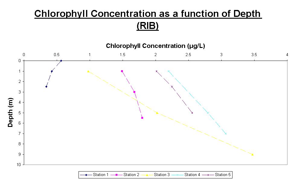
Fig 19 |
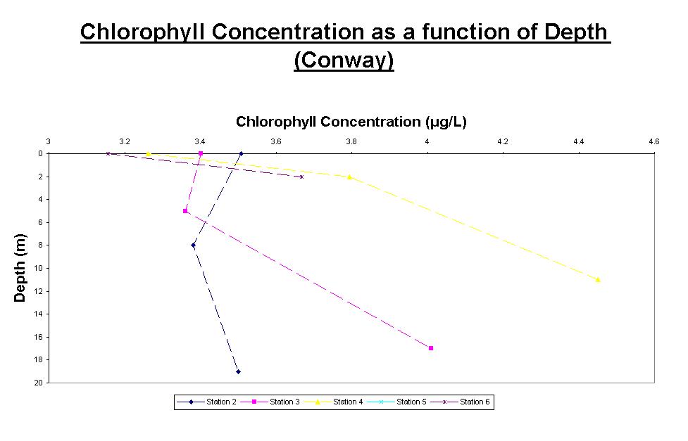
Fig 20 |
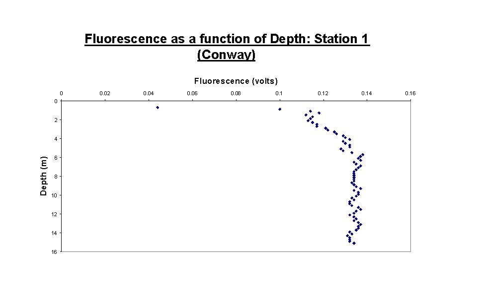
Fig 21 |
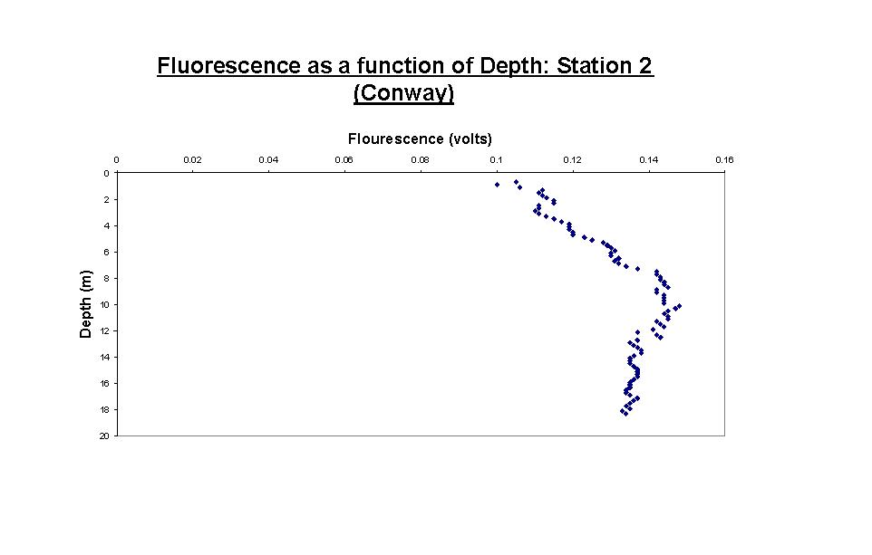
Fig 22 |
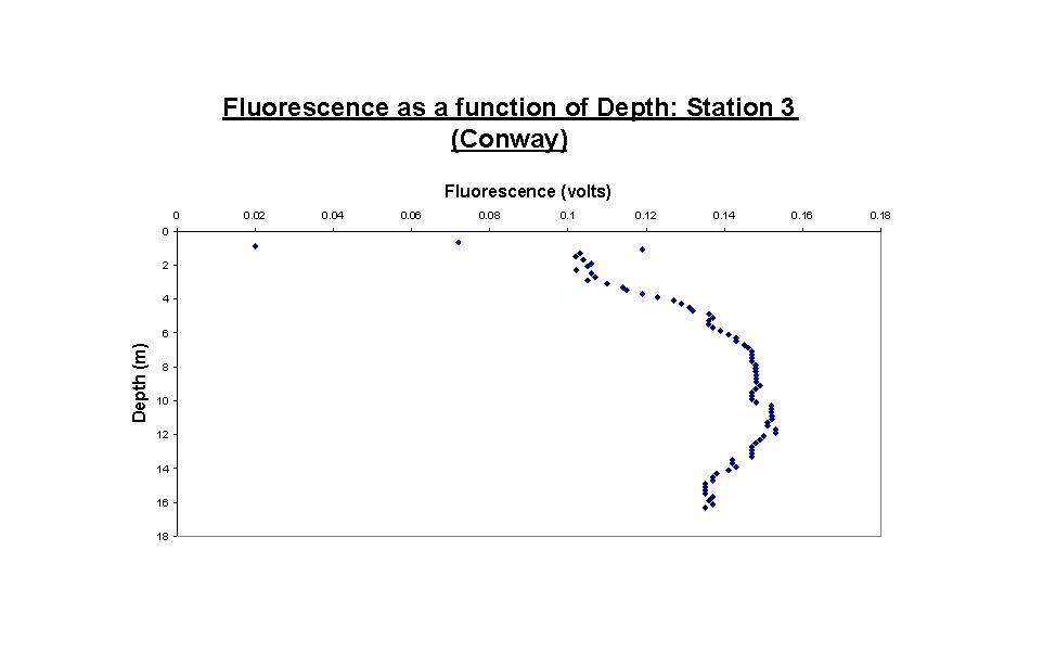
Fig 23 |
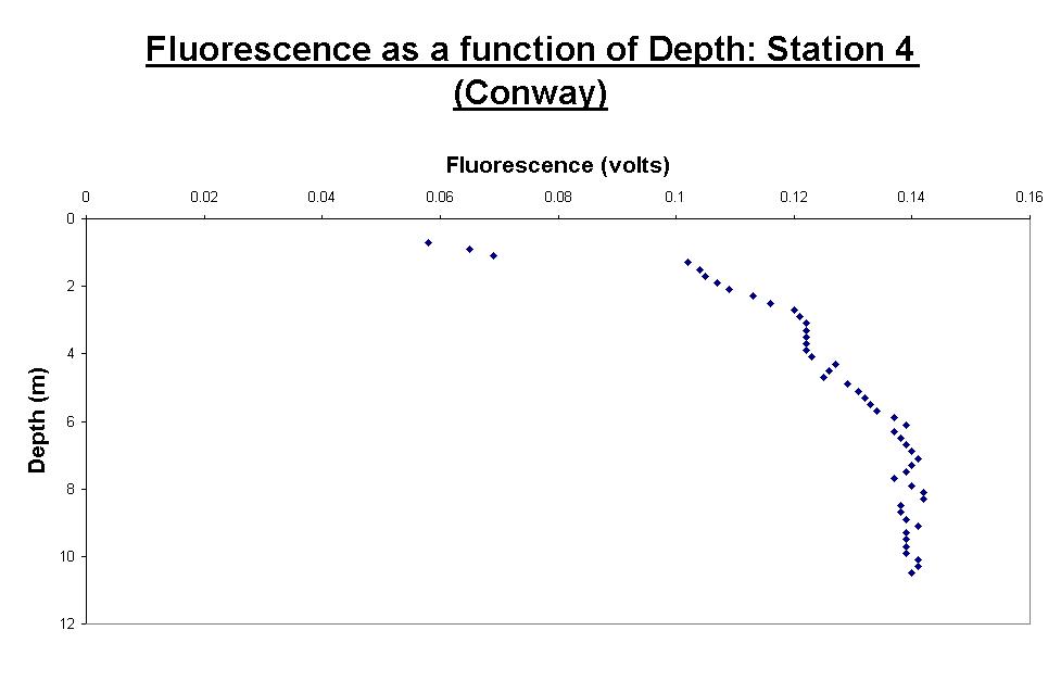
Fig 24 |
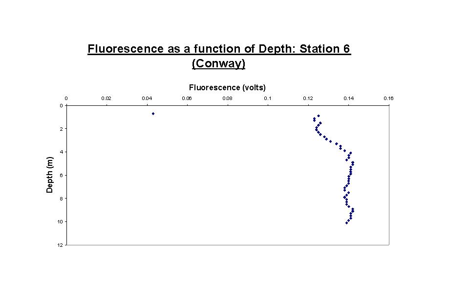
Fig 25 |
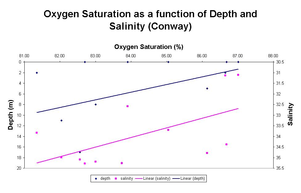
Fig 26 |
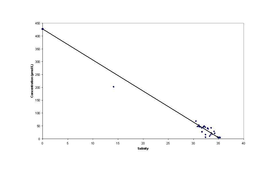 Fig 27. Nitrate mixing diagram
|
 Fig 28. Phosphate mixing diagram
|
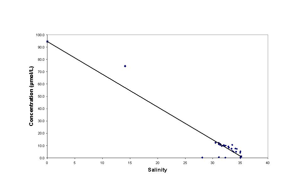 Fig 29. Silicate mixing diagram |
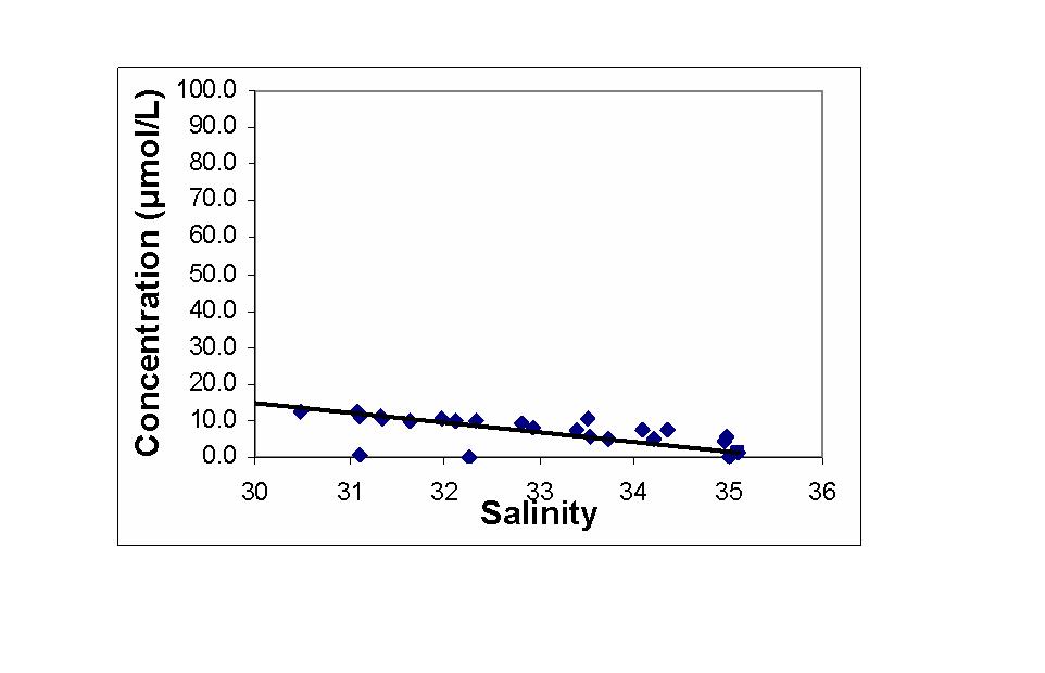
Fig 30. Concentration of Silicate against salinity
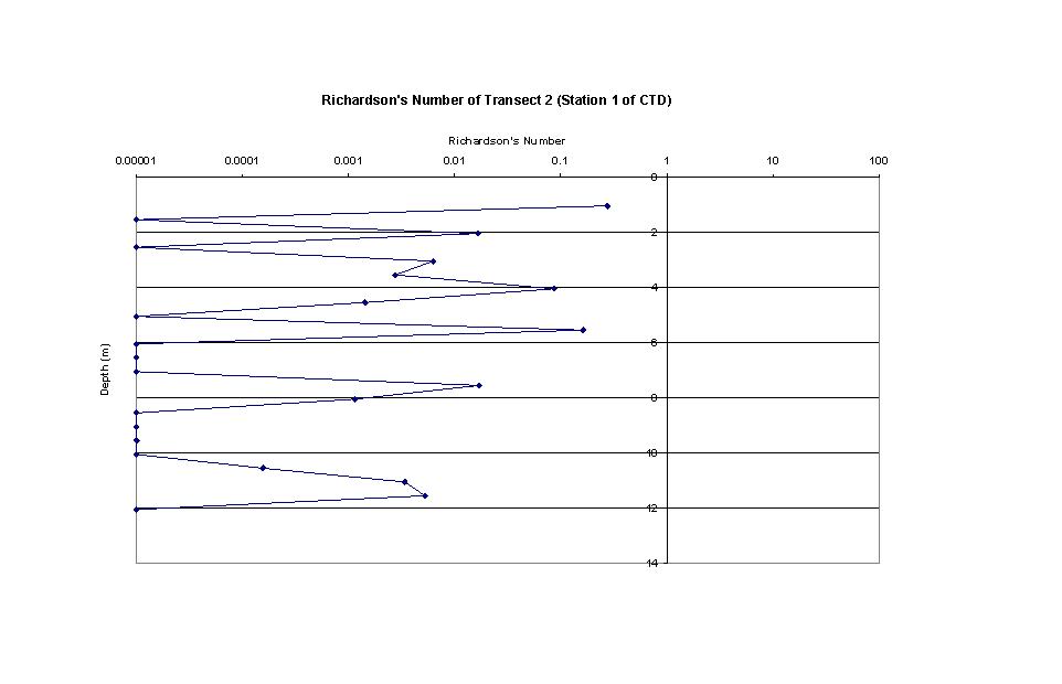
Fig 31
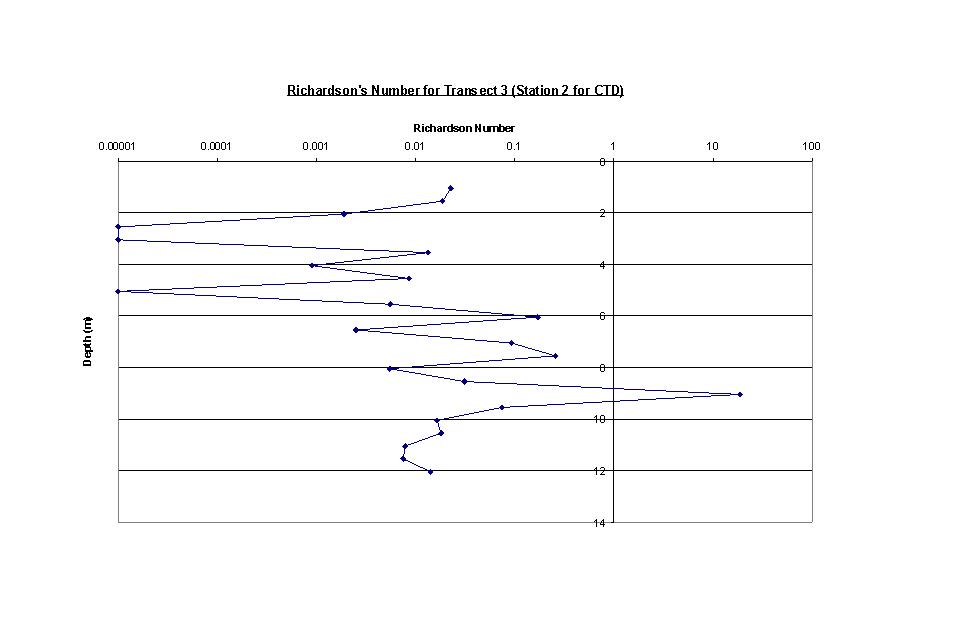
Fig 32
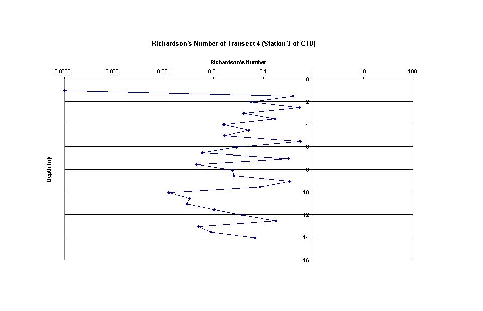
Fig 33
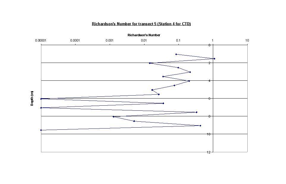
Fig 34
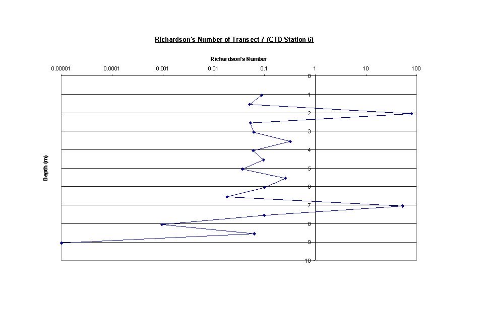
Fig 35
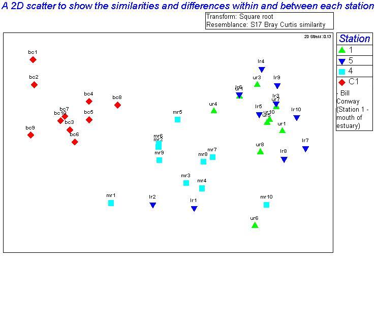
Fig 36
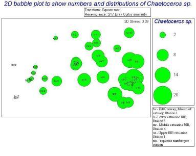
Fig 37
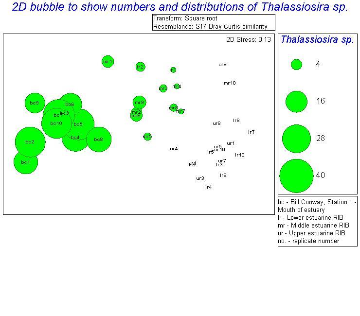
Fig 38
RIB secchi disc data;
|
Station Number |
Secchi depth (m) |
Euphotic zone (m) |
Water Column Depth (m) |
Irradiance |
|
1 |
2.4 |
7.2 |
4.9 |
3.5 |
|
2 |
1.5 |
4.5 |
7.5 |
2.2 |
|
3 |
1.4 |
4.2 |
9.9 |
2.0 |
|
4 |
2.0 |
5.9 |
13.5 |
2.8 |
|
5 |
2.5 |
7.5 |
6.6 |
3.6 |
Bill Conway secchi disc data;
|
Station Number |
Secchi depth (m) |
Euphotic zone (m) |
Water Column Depth (m) |
Irradiance |
|
1 |
2.4 |
7.2 |
4.9 |
3.5 |
|
2 |
1.5 |
4.5 |
7.5 |
2.2 |
|
3 |
1.4 |
4.2 |
9.9 |
2.0 |
|
4 |
2.0 |
5.9 |
13.5 |
2.8 |
|
5 |
2.5 |
7.5 |
6.6 |
3.6 |
Fig 39.
The aim of this survey was to collect biological, chemical and mixing parameters from the Fal estuary. These parameters included nutrients, chlorophyll, temperature and salinity. The group was split into two smaller groups, one on the RIB Ocean Adventure surveying the upper estuary and the other group on the RV Bill Conway surveying from the mouth of the estuary to the upper estuary.
Figure 1 shows the area surveyed by both vessels. The group on the RIB (Figure 2) sampled the upper estuary; At each station the RIB was moored and YSI probe was lowered through the water to give a vertical profile of the water column.
The group on the RV Bill Conway (Figure 3) sampled from the mouth of the estuary upstream towards the transect of the RIB. An ADCP (Acoustic Doppler Current Profiler) was used to create a horizontal profile of direction and speed of flow across the estuary, and a CTD to measure chemical and biological parameters.
Allocated Jobs
|
RIB: - PSO - Jonny Bliss - Data Recorder - Christina Wood - Deployer - Lorna Wrigley - Chemists - Sam Drawbridge
|
Bill Conway: - PSO - Cathrine Chatwine - CTD deployer - Molly Steele - Chemists - Chris Sturdy and Emma Rathbone - Data Recorder - Alex Lord - ADCP operator - Josh Georgiou |
Equipment used
- CTD (General Oceanics Inc. F7a)
-
Niskin sampling bottle model 1010-1.2 to 40L
-
Controller – Falmouth Scientific Inc. RMS MK VI 1015-PM
-
CTDave software
- ADCP – using WinRiver software
- T/S probe on Bill Conway – WTW ProfiLab LF597
- T/S probe on RIB – F598a Ocean Scientific International YSI probe
- Secchi disc
- Plankton net – 200 µm net, 50 cm mouth diameter, made by Duncan and associates.
-
Counter – HydroBios-Kiel
- NaviFisher software for navigation
Survey
The RV Bill Conway took six transects across the estuary, using an ADCP to create a horizontal profile of direction and speed of flow. The display of the vertical structure was used to decide where the CTD (Figure 4) vertical profile should be taken. Generally this was in the deepest part of the channel.
The CTD was used to sample at six stations throughout the Fal estuary, measuring temperature and salinity. Mounted to the CTD rosette was 6 Niskin bottles, which were used to take water samples at various depths in the water column. At each sampling depth, determined by the CTD profile, 2 water bottles were used for collection to ensure that if one bottle misfired there would still be a successful sample. These samples were divided into other bottles which were then used to measure chemical parameters – nitrate, phosphate, silicon and chlorophyll (Figure 5).
The YSI probe (Figure 6) used by group 2 measured temperature, salinity, pH, depth and oxygen concentration (as a percentage). Linear transects across the river were not used due to the effects of the wind and receding tide. These factors would have caused the RIB to drift significantly off course of the set transect, causing considerable inaccuracy in the results. After briefly analysing the results certain depths were chosen for water samples to be taken. These changed at each station due to depth of the water column and varying features, such as an obvious halocline or thermocline. This was accomplished by a Niskin bottle, which was triggered at a measured depth by a messenger weight. Different techniques (Figure 7) were used to store the water samples, with a view towards the factors needed for lab analysis the next day.
The Secchi disc was used to estimate the depth at each station of the euphotic zone (by multiplying the Secchi disc depth by 3). It was lowered into the water column until it was no longer visible, this depth being the Secchi depth.
Two zooplankton trawls (Figure 8) were conducted on the Conway, one at the site of the first transect near the mouth of the estuary, and the other further up the estuary. The net was towed for 4 minutes in each case, at a speed of between 1 and 1.5 knots. The net had a mesh of 200 µm, so was only suitable for collecting zooplankton rather than phytoplankton. Once on deck, the net was washed with seawater to ensure that all of the contents went into the collection bottle. After removing the bottle, formalin was added to preserve the sample.
After the CTD was back on board, water was collected from the Niskin bottles. The oxygen bottles (Figure 9) were filled with water direct from the Niskin bottle, using a tube which is slowly inserted to present air bubbles of excess mixing. The bottles were allowed to overflow reducing the possibility of air bubbles. The remaining water was then collected in a large bottle, which was first rinsed with some of the sample water.
The oxygen concentration was measured using the 14C method. The samples were prepared on the boat and the bottles were then placed in a bucket of seawater to alleviate the possibility that oxygen could seep in, i.e. in the case of the lid coming off.
The samples were filtered and added to glass nitrate bottles, plastic silicate bottles and glass oxygen bottles, ensuring the oxygen levels were preserved.
Water from the samples was passed through filters, to which acetone was added that preserves the phytoplankton. A zooplankton net was deployed at station 3, flow was also recorded. The contents of the zooplankton net were collected after 10 minutes hanging vertically in the water column and preserved with formalin.
The samples were taken back to the lab and analysed using various techniques (Figure 10, 11, 12)
Nitrate
Figure 13 shows that all of the RIB stations show a general decrease in the concentration of nitrate with depth showing fairly constant concentration until around 3 meters, when the concentration decreases sharply. The extent of depletion varies with position in the estuary with the least loss occurring in station 4. Station 1, located furthest up the estuary, has the highest nitrate concentration with a value of nearly 70μmol/L but decreases most rapidly with depth. The lowest concentration measured was in station 3 which was under 20μmol/L and was also the lowest depth sampled by 2 meters.
This graph (Figure 14) shows that in three Conway stations there was a decrease in the concentration of nitrate with depth. Two of the sampled stations are not included in the graphical representation, station 7 due to an extreme value of 202.35 which is presumed to be anomalous and makes the scale too large, and station 5 where no water samples were taken due to a Niskin bottle malfunction. Station 1 has the lowest nitrate concentration and was taken at the mouth of the estuary, however no lower values were taken due to technical difficulties with the CTD. Station 2 shows a gradual decrease in nitrate concentration with depth over a fairly small range due to a fairly low surface value. Station 3 and 4 both show a large nitrate loss over the first couple of meters depth, and then decrease far less rapidly for the remainder of the sampled points. Stations 2, 3 and 4, despite starting with a wide range of nitrate concentration, all show a final concentration of approximately 5μmol/L. Station 6 was only measured at the surface and 1 meter and showed no loss in nitrate concentration over this range.
Phosphate
Figure 15 shows that there are varying trends among the phosphate data between stations on the RIB. Station 1 has a clear, steady increase in phosphate concentrations as depth increases. However, station 2 first decreases and then increases to about half of the first concentration found. Station 3 shows yet another trend with a fairly steady decrease in phosphate concentration with depth. This could be due to the fact that the depths sampled were much deeper than the previous two stations. Station 4 where there is a large decrease in concentration between the first two depths, then a smaller decrease between the second and third depths sampled. Another trend is observed in Station 5 shows an opposite trend to station 2, with an initial increase and then a decrease to roughly double the first concentration found.
Figure 16 illustrates the phosphate data collected at each station on the Bill Conway. Since only one sample was collected at station 1, the comparison can be made across all stations on the surface. From this, it is seen that station 1 has the lowest phosphate concentrations, which could be due to the fact that it was taken from the mouth of the estuary. The other points don’t appear to be in any sort of order, which could be because they are all taken throughout a mixed estuary.
Station 2 shows a steady decrease in phosphate concentration, while station 3 has an initial increase, and then a decrease to approximately the same concentration as the sample taken from station 2 at depth. Station 4 shows a completely opposite trend of an increase in phosphate concentration. Stations 4 and 5 show very similar trend between their first two depths sampled, each showing a steady increase in phosphate concentration. Station 7 was also only sampled on the surface and was thus compared to all the other surface samples taken. It has the second highest phosphate concentration, behind station 2.
Silicate
According to the data taken by the RIB silicate concentration generally decreases with depth (Figure 17). In the case of stations 1 and 2, (taken at the head of the estuary) maximum silicate concentrations can be found just below the surface at around 1-3 meters with concentration of 12.1μmol/L and 10.1μmol/L increasing from a surface silicate concentration of 5.7μmol/L and 9.9μmol/L respectively. These then decrease to 12μmol/L at 2.5m (station1) and 5.5μmol/L at 5m depth (station2). Stations 3, 4 and 5 all have larger decrease in concentration from a depth of about 3-5m. Station 3 decreases from 11.5μmol/L to5μmol/L at 9m. Station 4 decreases from 11.3μmol/L to 8μmol/L at around 7m, and station 5 decreases from 9.8μmol/L to 7.7μmol/L.
As with data taken from the rib, all concentrations from each station decrease with depth (Figure 18). Station 1, measured at the mouth of the estuary has 0 concentration of silicate at the surface, however lack of data has led to an incomplete vertical silicate concentration profile. Station 2 is also incomplete, starting at a depth of 8m with a concentration of 4μmol/L, the silicate concentration then decreases to a minimum of 0.2μmol/L at 19m. Station 3 and 4 have very similar profiles, both starting at around 7.5μmol/L silicate concentration at the surface (0m) and then both decreasing, station 4 reaching a concentration near zero at 11m and station 3 reaching almost zero at around 10m. Station 6 again has an incomplete data set, beginning with a surface concentration of 11μmol/L silicate decrease to10.1μmol/L at 2 meters.
Chlorophyll
In Figures 19 and 20, chlorophyll is shown to increase with depth in almost all of the stations in both the RIB and Conway transects. Figure 19 shows that Station 1 in the RIB is the only station that shows a decrease in chlorophyll concentration with increasing depth. All other stations studied on the RIB show a positive trend, where chlorophyll concentration increases with increasing depth.
Figure 20 illustrates the data collected on the Bill Conway. Stations 2 and 3 show that chlorophyll concentrations are low initially, and then increase again at the deeper depths. The other stations all show that the chlorophyll steadily increases as depth increases.
Figures 21, 24 and 25 all show the basic trend that as depth increases, the fluorescence as measured by the fluorometer also increases. Another trend seen in these 3 graphs is that the fluorescence eventually reaches a point where it becomes fairly constant. This suggests that the amount of chlorophyll in the water column reaches a maximum and then becomes somewhat constant as depth increases. In each of these graphs, it is also observed that the chlorophyll concentrations become constant somewhere between 4 and 8 meters.
Figures 22 and 23 show a different trend. They both initially increase in the same manner as the other three figures, however between 10 and 12 meters, they start to decrease again rather than reach a constant chlorophyll concentration.
According to data (Figure 26), taken by both the RIB and the Conway oxygen saturation decreases with depth and salinity. Maximum oxygen saturation occurs at the surface with a value of 86.68%, saturation then decreases with depth to around 82.04% at around 11meters.
The Oxygen concentration also increases with salinity with a maximum saturation of 86.68% found at 34.4 salinity and a minimum oxygen saturation of 82.70 found at 35.3 salinity.
The nitrate concentrations largely fall below the TDL at salinities above 30, indicating non-conservative behaviour, namely removal in the lower part of the estuary (Figure 27). At salinity 14.1 there is a data point below the TDL, but on its own it is insufficient evidence of removal, and more samples would need to be taken to confirm this. As with the phosphate data, the reliability of the results and conclusions would be improved if more samples were taken at lower salinities.
Our graph shows a large deviation from the theoretical dilution line (a non-linear relationship), suggesting that phosphate behaves non-conservatively (Figure 28). The majority of the values lie above the TDL, suggesting that addition of phosphate occurs at high salinities towards the mouth, but there is insufficient data from lower salinities (from 0-30) to conclude this for sure. Normally, the riverine end member would be expected to have much higher phosphate concentration than the seawater end member. The value obtained in the lab seems much lower than it should be, but there was only one sample that could be tested. The validity of the TDL line relies on the accuracy of the end member concentrations, so it would be best to have carried out more sampling to confirm that the 0 salinity value is correct.
The silicate estuarine mixing diagram shows quite a strong linear relationship (Figure 29). River water contains much higher Si than seawater, and this is reflected in our data where the riverine end member has a far higher concentration than the high salinity samples. Silicate seems to behave conservatively as most points fall along the TDL. From the mixing diagram it appears at first that there may be some addition, however on inspection of an expanded section (between salinity 30 and 40) of the diagram (Figure 30) the data appears to fit the TDL quite well. At salinity 14.1, there is a point significantly above the TDL, but as this is the only data point it is not sufficient to conclude that there is addition of silicate at this point. At a few of our sampling sites silicate concentrations were found to be close to or at zero, which may indicate removal, however it is probably more likely that there was an error in the sampling or analysis in the lab, as in one case a concentration of 0.1 μmol/L was found at salinity 28, where it is very unusual to have such low silicate levels.
Estuarine Richardson graphs
(0.00001 has replaced 0 values as the log scale would not plot certain values)
The Richardson’s number is used to classify the stability of the water column:
Ri >1 = statically and dynamically stable
0< Ri <0.25 = mixing occurs (dynamically unstable, statically stable)
Ri <0 very unstable (dynamically and statically unstable)
Richardson’s number is worked out using ADCP data and the following equation:
Ri = -g/ρo [ (dp/dz) / (du/dz) ]
Ri = -g/ρo [ (ρ1-ρ2)/∆z ] / [ (u1-u2)/∆z ]
The expected pattern of our transects is well mixed at the mouth getting slightly more stratified higher up the estuary however because we sampled on the turning of the tide that was about to start its ebb flow this may not be the case.
Transect 2 – station 1 (Figure 31)
Looking at the temperature salinity graph for station 1 and the Richardson number (Ri) graph for transect 2 (station 1 for CTD), you can see that the water body is well mixed; this is expected as the profile was taken at the mouth of the estuary. This is shown by the Ri values all falling between 0.00001 and 0.28. The entire water column is dynamically unstable but is still statically stable. This corresponds well with the T-S profile, which shows that temperature and salinity are constant with depth.
Transect 3 – station 2 (Figure 32)
The Ri graph shows that there are two main layers in the water column, also seen in the T-S diagram. The upper layer is between 1.5m and 8m, with Ri numbers ranging from 0.00001 to 0.26 forming a well mixed water body. The lower layer begins at 10m down, and is again well mixed with values ranging between 0.01 and 0.1. These layers are divided by an area of the current that is statically and dynamically stable, with a Richardson’s number of ≈19 at 9.05m. No mixing occurs through or in this boundary, just above and below it. This boundary normally occurs due to the thermo- and halocline. Looking at the T/S profile the thermo- and halocline is between the depths of 8-10 m.
Transect 4 – station 3 (Figure 33)
The Ri graph shows a well mixed water body (with values of 0.00001 up to 0.54) but the Ri values are high compared to that of station 1 with a shallow thermocline and halocline occurring at ≈ 3.5m. This is due to the recent high precipitation freshwater input, high atmospheric temperatures heating up the surface layer and the turbulence of the lower layers pushing the thermocline and halocline.
Transect 5 – station 4 (Figure 34)
The Ri graph and the T/S profile at this station resemble the structure at station 3. Shallow thermo- and halocline being pushed up by turbulence, well mixed water body but at a depth of 1.8m (just above the thermocline) the Ri number increases to being over 1, which defines it as a stable layer of water, separating the mixing with atmosphere in the surface from the mixing below 1.8m. Overall the water body is predominantly well mixed.
Transect 7 – station 6 (Figure 35)
This station was the highest up in the estuary that the Bill Conway went. The graphs characteristically are showing stratification. The two spikes on the Ri graph show that the water column is split into 3 main water layers: the surface layer with low salinities and high temperatures down to 1.6m; the middle layer between 2.5m – 6.5m where salinities are increasing and temperatures are decreasing rapidly; and the lower layer from 7.5m down, where salinities reach their highest and temperatures reach their lowest. These layers are split and stopped from mixing together by layers of stable, non-mixing water. Shear occurs within the mixing layers maintaining the mixing and the stability of the high Ri numbers define the boundaries of these layers. The high Ri numbers of 79 and 53 occur at 2m and 7m depth, respectively, coincide with the two low gradient changes in the thermocline and halocline that occur. This stratification occurs due to the fresh water inputs on the river surface and seawater inputs tidally induced that underlie the fresh less dense water.
Plankton
The main group of phytoplankton found in the samples, which varied between the mouth and the head of the estuary were diatoms. They made up between 88.71 to 99.00% of the samples. Using PRIMER we distinguished the similarities and differences between the different types of phytoplankton at different locations within the estuary. Due to the fact that one of the replicate counts contained no species, it had to be discarded so that the other results were spread out equally and was clear; this anomaly is shown on the Bray Curtis similarity dendrogram. The Bray Curtis similarity dendrogram also established two main groups: the samples taken on the RIB and the samples taken on the Bill Conway. The 2D scatter (Figure 36) constructed shows that the data taken on the Bill Conway at the mouth of the estuary are considerably different from the data taken on the RIBs near the head of the estuary, with a significant increase in phytoplankton levels in samples collected from the mouth of the estuary. The 2D bubble plot (Figure 37) shows that Chaetoceros species is more dominant in the estuary compared to the mouth of the estuary, it is therefore a brackish species as the salinity there is between 30 and 31.5. The other 2D plot (Figure 38) shows that the Thalassiosira species is more dominant at the mouth of the estuary and very few existed in the samples near to the head of the estuary.
The majority of zooplankton recovered in the samples are copepods and copepod nauplii which have highest populations from the mouth to the middle of the estuary
Figure 39 shows the Secchi disc data for both RIB and Conway
The survey conducted in the Fal estuary shows a change in the chemical and physical characteristics from the head to the mouth of the estuary, which in turn affects the biological species inhabiting the area.
Nutrient inputs
Nutrient concentration changes with position and depth in the estuary. Generally nutrient concentration decreases towards the mouth of the estuary. Nitrate and phosphate enter the estuary through both point and diffuse sources. Point sources are anthropogenic and are generally consented discharges. They include sewage discharge, industrial effluent discharge, and input from fish farms. Diffuse sources can be natural or anthropogenic, such as run-off from the land, imports from offshore waters and N fixation by plants. Inputs of nutrients are dominated by diffuse sources, contributing 95% to N inputs, and 80% to P inputs, with the remaining amount via point sources. In the Fal estuary the data shows an increase in chlorophyll in surface waters towards the mouth, indicating an increase in the phytoplankton population leading to nutrient depletion. This is shown in figures (nitrate, phosphate and silicate with depth) by staggered surface concentrations increasing with distance from the mouth. The exception of this pattern is RIB station 3 having a higher concentration than RIB station 2 possibly due anthropogenic inputs or the ebb tide at the time of sampling causing the nutrients to move downstream.
Nitrate
Nitrate concentration decreases towards the mouth and the estuarine mixing diagram shows removal in the lower part of the estuary. Uptake of nitrate by phytoplankton is the most likely cause of the removal, as there are large blooms of diatoms during this time of the year. This is supported by the observation of large numbers of diatoms in water samples taken near the mouth of the estuary. The main input of N to the area is through the diffuse source of agricultural run-off into the rivers which feed the estuary with higher values found at lower salinities. The same point source pollution inputs near the mouth affect nitrate levels, so any especially high values which fall above the TDL may be due to increased pollution in that area. The main source of loss in the estuary can be accounted for by biological requirements of phytoplankton which becomes particularly significant with depth.
Silicate
Silicate surface concentrations decrease towards the mouth of the estuary due to the larger phytoplankton populations which incorporate silicate into their tests. As well as this silicate is depleted at the surface and increases in the water above and around the thermocline, followed by a decrease with depth, which could be related to the time of year. It is possible that around July the initial diatom bloom, comprising around 90% of the silicate in the water, would die and result in resuspension, increasing the concentration of silicate in the water column. The overall trend shown by the estuarine mixing diagram is of conservative behaviour. There is very little anthropogenic input of Si to the estuary so any changes will be due to the natural processes outlined above. There may be some addition near the mouth, possibly due to resuspension or input from pollution sources (e.g. chemicals used on boats).
Phosphate
Conversely phosphate surface concentration does not decrease with proximity to the mouth, where there is possible addition, which is likely to be accounted for by contamination from sewage from Falmouth docks with the main discharge sites located around Falmouth and Penryn, with few at the head of the estuary. This contributes to the relatively high phosphate levels around the mouth when compared to areas in the upper estuary. Another important source of phosphate is agricultural run-off, which could also help to create the high phosphate levels seen. The high levels also suggests that phosphate is not a limiting factor for phytoplankton blooms in the area as there is no loss in areas with the highest chlorophyll concentration.
Chlorophyll
Chlorophyll concentrations measured from samples show unexpected results with a decrease in concentration towards the thermocline between 4 and 8 meters and an increase below it. In a normal scenario chlorophyll reaches a maxima just below the thermocline and then would be followed by a decrease with depth. This could be a factor affecting the distribution of nutrients with depth, as stated above. Several factors could explain the unusual patterns shown. Firstly, in shallow areas of the estuary, light may not be a limiting factor in the growth of phytoplankton because the euphotic zone penetrates throughout the whole water column. This is the case in RIB stations 1 and 5. In other RIB stations the euphotic zone only extends for half of the water column, limiting the distribution of chlorophyll. At the Bill Conway stations the euphotic zone tends to be approximately half the depth of the water column allowing phytoplankton to survive above and below the thermocline. Station 4 of the Bill Conway sample appears to be significant as the depth of the water column is 4 times the euphotic zone depth, resulting in only a small part of the water column being available to phytoplankton. Also chlorophyll tends to be high where there is a large concentration of silicate which supports the data that diatoms are the dominant phytoplankton species at this time of year. It is possible that there are smaller than expected populations of phytoplankton in surface waters due to higher rates of predation by zooplankton and larger carnivores, making deeper waters more preferable for blooms. Similarly photoinhibition may play a part in limiting photosynthesis and influencing the distribution of phytoplankton populations.
Strangely the fluorometer data shows a decrease in chlorophyll with depth which contradicts the data collected in the samples collected. It is more likely that the fluorometer data are correct and that the discrepancy arose due to human error during collection or analysis. The data regarding fluorescence shows a chlorophyll maximum and thermocline at around 8 meters. At all stations there was a generally high oxygen concentration which decreased with depth and salinity. This insinuates that the water in the estuary is moderately healthy and contains relatively low populations of bacteria which deplete the water column of oxygen.
Physical structure
The physical structure of the estuary is shown to change throughout the estuary. At the mouth very little water movement was measured due to data being collected as the tide was turning, with the exception of the surface layer which has higher velocities due to wind speed. There is evidence of two distinct channels forming for the ebb and flow tides with the ebb tide moving out the left side of the estuary. This is probably due to the fact that the flows have differing strengths and are flowing over different topographies which allows each flow to carve out a separate route. The Richardson number calculated for this area shows the water column is very stable providing very good conditions for biological growth.
Phytoplankton
The phytoplankton observed vary with position and the characteristics outlined above with samples taken in similar locations containing similar proportions of species. However samples taken at the mouth of the estuary and the head are dramatically different in terms of the species found and the dominance. The dominant phytoplankton observed in the RIB samples are Chaetoceros spp, which differs from the samples taken at the mouth of the estuary, meaning they are more successful in estuarine waters. At the mouth of the estuary Thalassiosira sp. is the dominant species which implies they are more adapted to waters with a higher salinity. Both these phytoplankton are very similar so it is difficult to come to a conclusion as to why they would be distributed separately in the estuary. Both species tend to prefer lower levels of light and are affected by photoinhibition which produces the lower chlorophyll maximum observed in all stations. The sample had very high levels of phytoplankton implying that populations are large. Due to the time of year the samples were taken, these species are likely to be part of the summer bloom.
Zooplankton
Copepod nauplii are more abundant in the upper estuary than copepods probably because the populations in the more brackish parts of the estuary are likely to be in a different stage of their reproductive cycle which is more tolerant to changes in salinity. More copepods were found in the second zooplankton trawl in the mid estuary than at the mouth indicating conditions are more preferable for large zooplankton population. There are also noticeable differences between the proportions and compositions of zooplankton in the samples found at the mouth and measured by the RIBs.
Limitations
There are several limitations which have become evident upon analysis of the data. The program used to plot the biological graphs called ‘PRIMER’ requires a vast amount of data, which there was not time to sample. This produced graphs which do not show the data as efficiently as would have been preferable. Also with regards to the estuarine mixing diagrams, more replicates should have been taken for the riverine end member and at lower salinities as the theoretical dilution line is not very accurate. This has to be taken into consideration when drawing conclusions from the data. The graphs produced to demonstrate the chemical properties of the estuary have had lines added to connect the points at each station. This is not a representative curve of changes with depth and has only been added for ease of viewing the different stations. Unfortunately there was not enough time or manpower to survey as extensively as is required to draw any definite conclusions about the properties of the estuary. If more time was available samples would be taken systematically at a variety of depths to give a more accurate profile of the structure and the changes taking place with progression along the estuary. As well as this it would have been beneficial to sample in all the rivers and creeks which input material into the estuary to determine the major fluxes of nutrients into the estuary.
Date: 10/07/07
Tides: HW 4.5m 00.21GMT, LW 1.6m 07.06GMT, HW 4.5m 13.06GMT, LW 1.7m 19.44GMT
Boats: RV Callista
PSO: Chris Sturdy
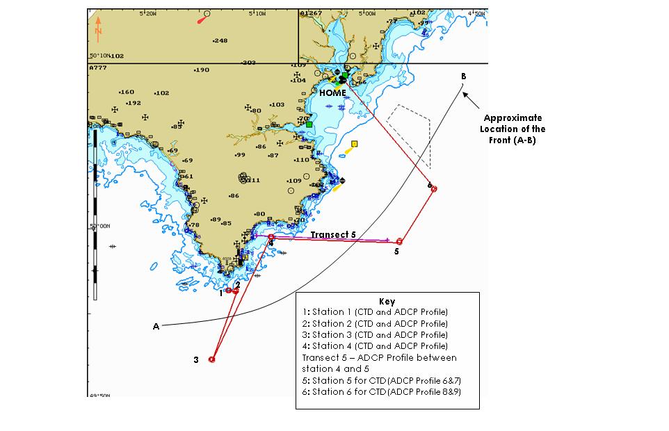
Fig 1. Offshore transect
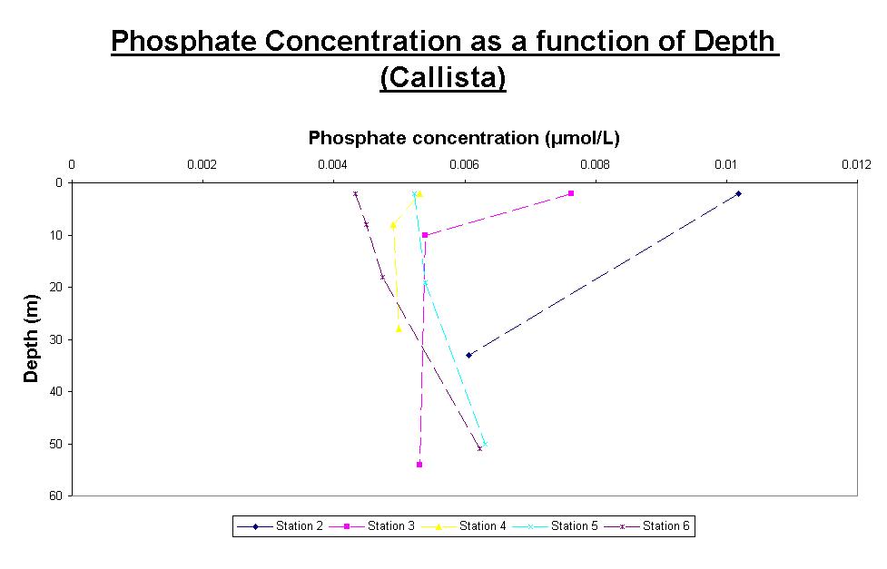
Fig 2
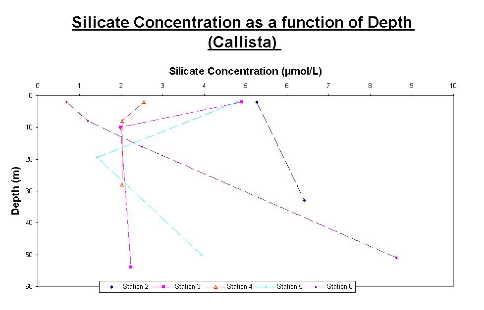
Fig 3
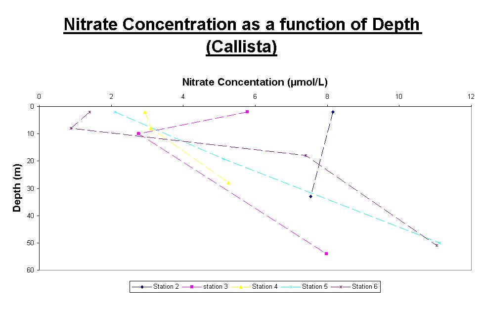
Fig 4
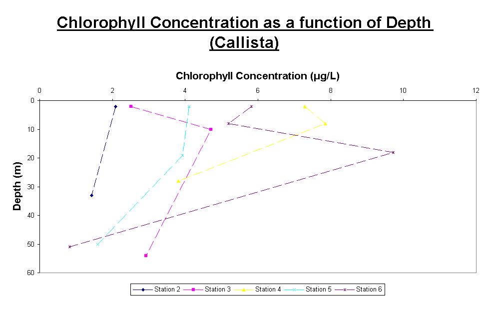
Fig 5
Fig 6
Fig 7
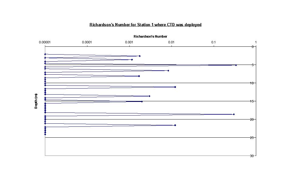
Fig 8
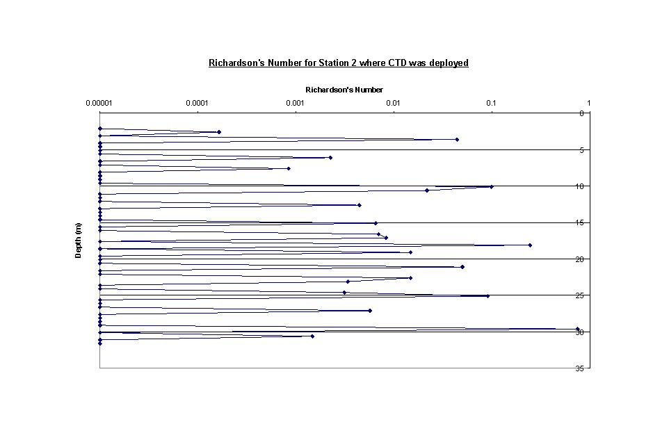
Fig 9
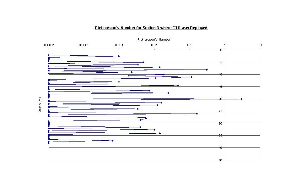
Fig 10
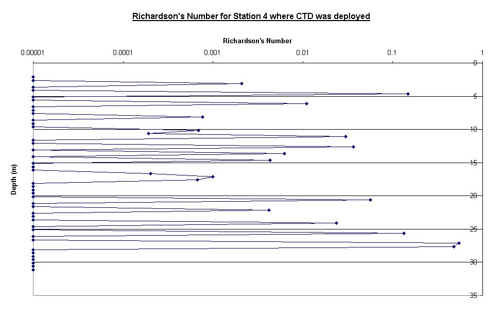
Fig 11
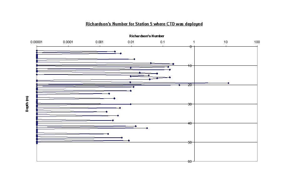
Fig 12
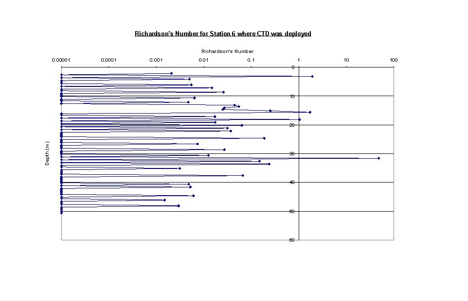
Fig 13
Callista Secchi disk data;
|
Station Number |
Corrected Secchi depth (m) |
Euphotic zone (m) |
Water Column Depth (m) |
Irradiance (m) |
|
1 |
7 |
21 |
34.2 |
10.1 |
|
2 |
7 |
21 |
33 |
10.1 |
|
3 |
8 |
24 |
78 |
11.5 |
|
4 |
5.6 |
16.8 |
19.9 |
8.1 |
|
5 |
6 |
18 |
73.7 |
8.6 |
|
6 |
5.5 |
16.5 |
69.7 |
7.9 |
Fig 14
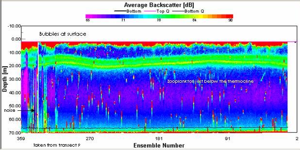
Fig 15. ADCP Backscatter
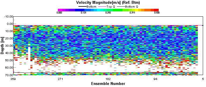
Fig 16. Velocity Profile
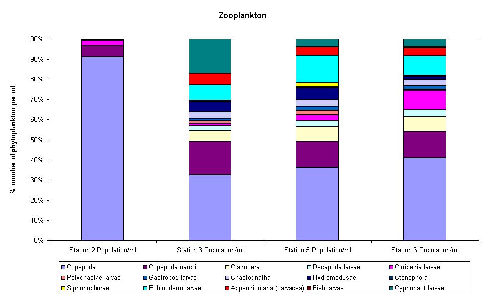
Fig 17. Zooplankton bar chart
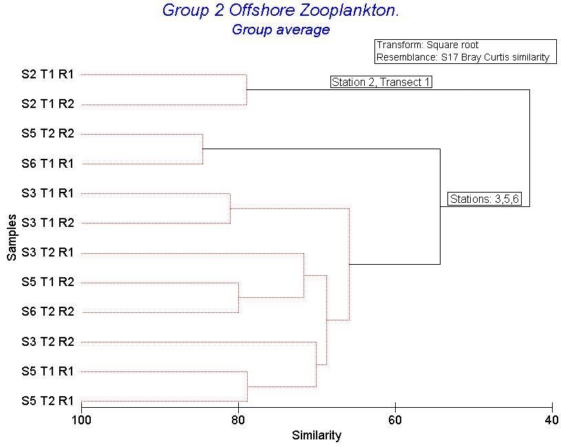
Fig 18. Bray Curtis Dendrogram
We were aiming to investigate the difference in water column structure between offshore sites and those closer to the coast/the estuary. By measuring temperature and salinity with depth, this structure can be observed. Water samples taken at depths (chosen after examining the temperature/salinity profiles) can be used to examine the chemical and biological distributions in the water column also.
At this time of the year, there is a marked difference in physical, chemical and biological structure between coastal waters and offshore waters. Knowledge of similar areas suggested that the coastal sites would show a well-mixed water column with no obvious thermocline, but that there would be thermal stratification of the offshore sites due to increased irradiance in the summer. The typical structure of offshore waters at this time of year is an upper mixed layer and a lower mixed layer separated by a thermocline. The ADCP was used to give a picture of the physical circulation of the water, by measuring currents and flow. A CTD was used at chosen stations to take a vertical profile of temperature and salinity. This enabled us to identify the location of the thermocline (if present) and aid in our decision of where to take water samples. After looking at the CTD profile, Niskin bottles were used at various depths at each station, for example at the depth of the thermocline. These samples were used to measure nutrient (N,P,Si) concentrations, as well as dissolved oxygen and chlorophyll. The CTD also monitored fluorescence, which is another measure of chlorophyll in the water column. In the lab, phytoplankton from the water samples were examined and counted, as were zooplankton, which had been collected during plankton trawls at some of the CTD stations.
We started our survey (Figure 1) at Lizard Point, aiming to arrive at 10.30 GMT at a slack tide for ease of sampling as multiple currents converge at that point. From this point we worked further offshore and at sites of interest heading east towards Falmouth parallel to the shore to the next station, before heading back towards shore for the next station. We then headed back out to sea whilst performing an ADCP survey in an attempt to locate the tidal front. Two more stations were sampled on the way back to Falmouth.
Seven stations were sampled with a CTD Rosette with Niskin bottles, transmissometer and flurometer. On the downcast of the CTD the vertical structure of the water column was assessed allowing us to choose depths to sample with the Niskin bottle. On all but the second and seventh stations the Niskin bottle samples were taken above, below and in the theromocline. Station 2 showed no or very little thermal structure so Niskin samples were only taken at the surface and lowest point. On the seventh station 4 samples were taken. In addition to samples relative to the thermocline a fourth Niskin bottle was taken at 8m because the transmissometer showed possible signs of a coccolithophore population. At each station an ADCP profile was taken to allow analysis of the vertical structure and stability of the water column. A Secchi disc was also used to estimate the depth of the euphotic zone at each station.
At every site sampled with a Niskin bottle the recommended procedure was followed to obtain samples to be analysed to determine O2 concentration, nitrate, phosphate, silicate and chlorophyll. Also samples were taken and preserved to determine the phyto- and zooplankton populations in the chosen areas.
Phosphate
Figure 2 shows that all the values observed for phosphate are very low with the maximum concentration being around 0.01µmol/L and a minimum concentration of around 0.004µmol/L. Given that these are the extreme values, this only covers a range of 0.006µmol/L. Stations 5 and 6 have a constant increase in concentration down to a depth of 50meters and were the two stations which seemed to be on the stratified side of the tidal front. Station 3 has a relatively high concentration of phosphate in the surface waters, but decreases rapidly from 0.075µmol/L to 0.055µmol/L in the top 10 meters approaching the depth of the thermocline. This value then seems to remain constant throughout the water column to a depth of 55 meters. Station 2 shows the greatest change between surface and depth of approximately 0.004µmol/L.
Silicate
According to Niskin bottle samples taken throughout the water column at certain stations offshore, silicate concentrations vary drastically depending on depth and position (Figure 3). Station2 has a surface (2m depth) concentration of 5.2μmol/L which increases to 6.22μmol/L at depth 32m. The concentration of silicate at station3 decreases at first from 4.92μmol/L at surface to 2μmol/L at 10m. It then increases to 2.2 remaining relatively steady through the water column to about 55m. Station 4 again decreases at first from a surface concentration of 2.5μmol/L to a minimum concentration of 2μmol/L at about 10m. The concentration then remains constant throughout the water column to a depth of 28m. Station 5 has a surface concentration of 4.9μmol/L, the concentration then decreases to 1.8μmol/L at 20m and then rises to a concentration of 4μmol/L at a depth of 50meters. Silicate concentrations at station 6 increases dramatically through the water column, starting with a surface concentration of almost zero, the amount of silicon increases almost proportionally to a concentration of 9μmol/L at 50meters.
Nitrate
In Figure 4 the nitrate concentrations, especially at stations 3, 4 and 5, show an almost directly opposite pattern to the concentration of chlorophyll shown in Figure 5. Station 2 shows a relatively constant small decrease in the concentration of nitrate from around 8uM to around 7uM over the sampled depth of 32 meters due to the lack of stratification in the water column. Station 3 nitrate decreases from the surface to the thermocline by 2uM, then increases with depth to 8uM by 54meters. This is quite a typical pattern shown in offshore summer stratified waters with the nutrients being depleted around the chlorophyll maximum and increasing with depth as light becomes the limiting factor for growth. Another example of nutrient distribution in stratified waters is shown by station 5 which has a very low nitrate concentration of 2uM in surface waters. This increases at around 18 meters below the chlorophyll maximum where nutrients are mixed upwards by shear stress but light penetration still allows growth, this then continues to increase in deeper water where nutrients are not depleted. The general trend of Station 4 is a constant increase in nitrate concentration down to a shallower depth of 29 meters. At station 6 we took 4 samples and the graph shows that this allowed us to make a much more accurate prediction of the chemical and physical properties of the surface waters. This is demonstrated by the decrease in nitrate in the top 10 meters which would not have been represented had we followed our original sampling procedure.
Chlorophyll
Station 2 (Figure 5), sampled at Lizard Point, showed no evidence of a thermocline and thus chlorophyll decreases gradually with depth until the maximum depth sampled depth of 32 meters. Station 3, 4 and 6 all show an increase in chlorophyll concentration in the region of the thermocline located at 10 meters, 9 meters and 19 meters respectively. These three stations all show a classic chlorophyll maximum just below the thermocline which is characteristic of stratified waters. This change was shown in station 4 but to a lesser extent with a change of 0.5µg/L as compared to almost 5µg/L at station 6. This station also showed a rapid decrease in the concentration of chlorophyll below the thermocline of around 9µg/L until the measured depth of 51 meters. All other stations with a thermocline present showed this pattern but to a lesser extent with the smallest decrease being around 2µg/L in station 3.
Temperature/salinity profiles
Inshore stations such as Station 1 which was very close to the coast, showed no real change in temperature or salinity with depth (Figure 6). Temperature remains consistent at 13.2 oC through the whole water column. Fluorescence is low at the surface but increases to a consistent level below 10m.
Offshore stations, for example Station 5 showed clear thermal stratification (Figure 7), with warm (14oC) surface waters, a sharp thermocline between 17 and 20m, and then a temperature drop to a constant 12.8 oC. A halocline is present at the same depth as the thermocline. Low fluorescence at the surface, but a large spike at the thermocline.
Offshore Richardson graphs
The expected pattern was that the water column would be seen to be well mixed nearer the coast, with an increase in thermal stratification with increasing distance offshore. It was also expected that mixing would be most noticeable at the first station, off Lizard Point, as the headland is a place where 2 currents from either side converge.
Station 1 – Transect 1 (Figure 8)
Looking at the temperature salinity graph for station 1 and the Richardson graph for transect 1, it can be seen that the water body is well mixed. This is shown by the Ri numbers, which are all between 0.00001 and 0.15. This shows that the water column is statically stable, but dynamically unstable. This is expected as station 1 and transect 1 were located off the headland at Lizard Point, where mixing was increased due to the 2 converging currents in the area.
Station 2 – Transect 2 (Figure 9)
The Ri and T/S graphs for this station, show that the water column in this area is also well mixed. Station 2 was located very close to station 1, therefore the results obtained are to be expected.
At a depth of around 30m the water body appears to be slightly more stable (Ri = 0.9) than the rest of the water column (Ri = 0.00001 to 0.25). This is also shown in the T/S profile with temperature decreasing from 13.2oC to 13.1 oC, whilst salinity increases slightly.
Station 3 – Transect 3 (Figure 10)
The graphs for station 3 show that there are 2 water bodies present. The first, upper body spans 19m down from the surface. The second, lower body begins at 21m and continues to the sea bed. This is depicted in the Ri graph, with a stable Ri number of 2.98, showing the whereabouts of the thermocline. This is confirmed by the T/S profile, with temperature decreasing from 14.0oC to 12.7oC and a slight increase in salinity.
The results for this station agree with the initial expectation that the thermocline is more developed offshore as mixing is less prominent.
Station 4 – Transect 4 (Figure 11)
The results show that the water column at station 4 is generally well mixed, with an increase in stability at a depth of 27m (Ri = 0.54). Again, this is to be expected as this station was located near the shore, north east of Lizard Point, however it can be seen that the water column is not as well mixed as that at station 1 as the area is more sheltered. This is backed up by the T/S profile, which shows a slight decrease in temperature between 11m and 20m.
Station 5 – Transect 6 (Figure 12)
Station 5 was located offshore, east of station 4. The results obtained, show that the water column in this area is composed of 2 main bodies, one upper (above 19m) and one lower (below 20m). This is confirmed by a picnocline that can be seen at approximately 20m on the T/S profile.
The two bodies of water are split by a stable Ri value of 11.94. The upper body is well mixed, shown by Ri values ranging from 0.00001 to 0.21, with the lower body being relatively more unstable, with Ri values between 0.00001 and 0.03.
Station 6 – Transect 8 (Figure 13)
The water column appears to be well mixed, however there does appear to be some structure to the water body as shown by the values of the Ri number, when they increase above 1.0. One would not expect stratification of more than two layers to occur in this area as it is offshore, however it appears that the water column is split into more than two layers and this could be due to drifting during surveying.
The T/S profile for this station shows the presence of a thermocline at approximately 20m. This is not backed up by the Ri numbers, although a more stable layer is seen at around 30m.
ADCP
This cross section (Figure 15) shows the amount of backscatter received by the ADCP. There is a large amount of backscatter from the surface of the water, which may be caused by bubbles from waves or from the wake of the boat. Transect 9 clearly shows shoals of fish of varying sizes and a band of zooplankton near the surface. From this you can predict where the thermocline (or even pycnocline) may reside. In the far left hand side of the image there appears to be some noise, which has distorted the record of the ADCP. Just above the sea floor (the thick black line) there is some strong backscatter which is caused by the ADCP; there is a boundary above the sea floor (the thin black line) of which you discount any backscatter below it due to inaccuracy
Figure 16 shows the velocity within the water column, there is a slightly higher velocity at the surface above the thermocline shown above.
Zooplankton
The zooplankton samples consisted mainly of copepods with some copepod nauplii. This can be seen in Figure 17. It also shows that station 3, 5 and 6 have similar proportions of the same species. Station 2 is made up of 90% copepoda. Station 2 is significantly different from the other stations (group average). Figure 18 also shows that station 2 is the most different. The PRIMER graphs also show that Station 5, Transect 2 and Station 6, Transect 1 are significantly different but are more similar to stations 3, 5 and 6 than to station 2. Figures (bubble charts copepod and cyphonaut larvae) show that Station 2 contains the largest number of copepod species and no cyphonaut larvae.
The area offshore adjacent to Falmouth estuary has a defined physical structure caused by the formation of a front, which dictates the chemical and biological properties. The front forms a barrier separating the mixed estuarine water and the seasonally stratified open water, thus preventing small organisms and nutrients from traversing from one water body to another. The front is likely to be caused where the extent of tidal mixing from the estuary is not enough to overcome the increasingly buoyant layer of stratification, which is heated by solar radiation. Conversely there is a strong thermocline creating the distinct stratification.
Nitrate
Nitrate concentration in the offshore areas follows the typical pattern observed in stratified waters, showing a trend of increasing concentration with depth and depletion of nitrate around the thermocline. There is then an increased concentration at depth where phytoplankton activity does not diminish the levels of nitrate. This is demonstrated in stations 3 and 6 where the likely cause of depletion in the surface waters is utilisation by phytoplankton during the large blooms which occur in the spring and summer. Station 5 would be expected to have similar properties to stations 3 and 6 as they were both taken in areas with similar water column properties. However, as the data sampled to represent the thermocline appears to be lower than the other samples taken, it is possible that sampling occurred below the euphotic zone explaining this discrepancy.
The dominant blooms in these areas are located in or just below the thermocline between 10 and 20 meters where shear stress causes some upward mixing of nutrients. Station 2 showed a relatively small change in the concentration which indicates a well mixed water column. The likely cause for this is that station 2 is located just offshore of Lizard Point which occurs on a convergence of two currents which promotes mixing.
Silicate
Silicate concentration shows a similar pattern to that exhibited by nitrate with the offshore sites (3, 5, 6) showing significant stratification. This is shown by a sharp decrease in the concentration around the thermocline with all the offshore stations showing a decrease below 3 μmol/L. The acute decrease around the thermocline indicates that diatoms are the dominant phytoplankton group, as they require a vast amount of silicate. Again station 2 shows a completely different pattern than all the other stations as there was not a thermocline so generally silicate is depleted in the surface waters and increases with depth. Similarly station 4 does not show a decrease in the silicate concentration around the thermocline, again implying that the water column in this area is well mixed.
Phosphate
Phosphate concentrations are very small over all the stations sampled when compared to the values observed within the estuary. This is probably due to the large amount of phosphate input by anthropogenic sources at various points throughout the estuary. The changes observed in phosphate concentration occur over a very small scale with a maximum change of 0.004 μmol/L in station 2. Stations 6 and 5 show an increase in phosphate concentration with depth, reinforcing the theory of stratification in the water column. Conversely stations 4 and 2 show a decrease in concentration with depth due to the upward mixing in samples taken closer to the shore.
Chlorophyll
The concentration of chlorophyll shows a distinct pattern of sharp increase at, and directly below the thermocline in stations 6 and 3 and a decrease with depth. Station 5 would be expected to follow the same pattern shown in offshore areas however the second sample was taken at a depth below the euphotic zone, meaning that light would be a limiting factor in the growth of phytoplankton. This would explain the lack of an increase in chlorophyll concentration. The depth of the euphotic zone at stations closer to the shore indicate that they occupy a large proportion of the water column resulting in little limitation by light. In the offshore stations the euphotic zone only penetrates into the upper 20 meters of the water column so light limits the depth phytoplankton can bloom at maintaining nutrient concentrations below the thermocline.
The formation of a thermocline explains the low fluorescence at the surface, as the phytoplankton have depleted the nutrient supply. At the offshore stations, fluorescence reaches a maximum at the thermocline. This provides the best conditions for growth, as there is sufficient irradiance and also a supply of nutrients via upwelling from deep mixing. Fluorescence declines with depth after this, as growth becomes light-limited. The stations close to the coast are well-mixed with homogeneous water in terms of temperature and salinity. Stations 1 and 2 show little variation in fluorescence with depth, with the exception of lower values at the surface. This is typical of summer coastal waters, where phytoplankton deplete nutrients to the extent that they become growth-limiting.
Physical structure
The physical structure is very distinct and varies depending on location relative to the front. Offshore stations show two prominent layers with a very high Richardson number implying a very high stability. This is also reflected in the distribution of nutrients and chlorophyll with high nutrients below the thermocline and evidence of large populations of phytoplankton in the surface layer. The exception to this is station 6 which does not show the expected vertical profile despite it being prominent on the CTD data. The contradiction in evidence could be due to sampling closer to the front than was intended which would include more of the mixed water body.
Phytoplankton
The dominant phytoplankton species found in all stations were the diatoms Chaetaceros which require low levels of silicate and reside around the thermocline due to intolerance to irradiance. Station 2 was the only station that showed a different composition with a wider diversity of organisms and a sample which was not dominated by Chaetaceros. This is probably due to the convergence of water masses containing more types of phytoplankton and more nutrients available for fixation due to mixing.
Limitations
There were many limitations with regards to our survey of the offshore areas. Only two samples were taken in station 2 due to the lack of a thermocline measured by the CTD. However if more time was available samples would have been taken at various depths throughout the water column to give a more accurate depiction of the structure of the water column. The lack of chlorophyll maxima in station 5 implies that water was sampled too far below the thermocline to give a portrayal of the phytoplankton and nutrient distribution. Also as we were quite far offshore the sea was fairly rough which made our measured depths quite inaccurate and did not allow enough samples to get a thorough water column profile. The primer graphs do not depict the zooplankton samples very well due to the lack of data, where primer requires vast amounts of data which there was not time to sample. Another concern is that during sampling there was drifting of the boat causing inaccurate locations and thus conclusions.
As can be seen from the data obtained throughout this field study, the Fal estuary is a vast and diverse environment. Whilst looking at the physical, chemical, biological and geophysical aspects of the estuary, many observations were made. The salinity, chlorophyll concentrations, nutrient concentrations, oxygen saturation and depth were measured at numerous stations throughout the estuary and later examined. These samples were analysed and plotted so that trends in the data could be observed. The data showed many conclusive trends, as well as many trends that were not expected. Overall, we suggest that more sampling needs to be conducted in the estuary in order to make any more detailed conclusions. Whilst our sampling was fairly complete, more sampling would have provided better profiles of the estuary. Weather was also a major aspect in our sampling procedures. It also limited the areas of the estuary that were able to be sampled, as well as the areas offshore that were accessible.