Aislinn Sinclair ~ Ben Hume ~ Tom Dynes ~ Laurie Casburn ~ Claire Finney ~ Dan Hawes ~ Matt Taylor ~ Tom Southall ~ Emma Oastler ~ Lizzy McMichael ~ Jessica Griffiths

Introduction

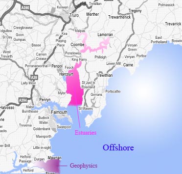
Welcome to Group 1's Falmouth Field Course Web Page! During the first two weeks in July 2007, 11 oceanographers from Southampton University conducted a wide variety of research in and around the Fal Estuary system. Large amounts of data were collected covering the biological, chemical, physical and geophysical aspects of the area, and the interaction between them. The map below illustrates the different locations that our research focused on over the two weeks.

Map showing the general location of the 3 areas of research

This website presents a summary of the initial findings. It has been divided into 3 sections, each covering a certain aspect of our work.

Back to Top

Background

The Fal estuary is located on the south coast of Cornwall (S.W. England) at the Western entrance to the English Channel. As well as being a natural harbour, the Fal is a good example of a ria, forming at the end of the last ice age due to sea level rise. The main source of freshwater to the estuary is the Helford river and tributaries including Restronguet creek and the Carnon River deliver freshwater of different biochemical composition. Being a macro tidal estuary with a spring tide of 5.3m, it characteristically has a lot of tidal flat and salt marsh habitat (93ha of salt marsh).

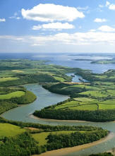
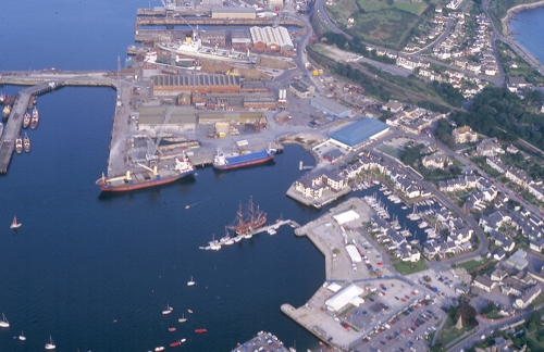
The River Fal flowing into Carrick Roads

The environment changes from high energy rocky shore at the mouth to low-energy soft sediments further upstream producing a diverse range of habitats. The Gulf Stream and prevailing winds approach England from the South-West which creates a warm, windy climate: mean summer sea temperature in The Fal is 16 ºC and waves exceed 3m for 10% of the time.  The geology of the shoreline around the Fal is Devonian sedimentary rocks with Carnmenellis granite to the west and St. Austell granite to the east.

Falmouth is one of the main docks for the S.W. coast and has been classified by MAFF (Ministry of Agriculture, Fishery and Food) as a major port.  Associated disturbances to the estuary include dredging activities, antifouling and the release of oil and sewage.  Fishing is carried out all year both inshore and offshore as well as digging in the muddy sediments for bait.  Mussels are cultivated on ropes from pontoons in the King Harry Passage area. Maerl is commercially valuable and is cultivated in the Fal for use in agriculture.  A license issued by the Crown Estate Commissioners allows 30,000 tonnes of dead maerl to be dredged from the Fal estuary each year.  However, there is a concern that the fragile and rare live maerl is present in the beds of dead maerl where the dredging is carried out.

Falmouth Docks

 Sandbanks in the Fal are of national importance due to the presence of both eelgrass Zostera marina beds and maerl beds.  The Fal and Helford are protected by the JNCC (Joint Nature Conservation Committee) and are Special Areas of Conservation (SAC) sites. St Mawes Bank is the largest (approx 150 ha) bed of living maerl in England and Wales.   Maerl grows in nodules that form a lattice structure, providing habitats and substrata for various species of infauna and epifauna such as the rare Couch’s goby (Gobius Couchi). Juvenile edible crabs and bass spend the early stage of their life in The Fal and from June areas are designated bass nursery grounds and angling restrictions imposed.

 Incidences of phytoplankton paralytic shellfish poisoning (PSP) have occurred following toxic summer blooms of Alexandrium tamarense in the Fal estuary.  High nutrient levels triggering the blooms may be due to increased sewage input during the tourist season.  Diarrhoeic shellfish poisons (DSP) and Amnesic shellfish poisoning (ASP) have also been related to causative algal species present in the Fal estuary. 

Mining for metalliferous deposits has been a feature of the catchment since the Bronze Age.  Although the last active mine (Wheal Jane) was abandoned in 1991 heavy metals deposits still contaminate sediment in the Fal estuary, making Restronguet Creek the most metal polluted in the U.K (Somerfield et al., 1994’ ).  The tributary Carnon River contains high concentrations of certain metals: Zn, Fe, Mn, Cu, As and Cd.  The Carnon River drains to the Restronguet creek where levels of fauna have found to be considerably lower than that in other parts of the estuary.  The only bivalve known to survive the toxic conditions is scrobicularia plana.  However, certain species have developed strains tolerant to Cu and Zn, such as nereis diversicolor.  Extraction of china clay has increased the input of fine sediment, leading to silting.  The anthropogenic impact on the Fal has led to the area being a focus of scientific studies.

Aerial photograph of Restronguet Creek during the Wheal Jane mining incident, January 1991

Back to Top

Introduction - Offshore Processes

R.V. Callista

Tuesday 3^rd July 2007

Aim:

• To gain a better physical, chemical and biological understanding of the waters offshore from Falmouth, and to assess the extent to which vertical mixing has an effect on planktonic communities.

Objectives:

•  To collect a data set which gives an accurate depiction of the waters offshore from the Fal Estuary.

• Through the use of ADCP transects and CTD profiles, quantify the vertical structure of the water column, and the presence of a seasonal thermocline.

• To study the taxonomy and abundance of phytoplankton and zooplankton communities within the water column.

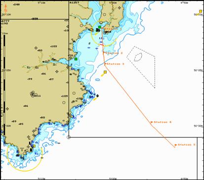
Research was carried out aboard the R.V. Callista. The weather was forecast to be rough, with F5 Westerly winds expected later in the day. 5 stations were sampled, starting at Black Rock which is located at the mouth of the Falmouth Estuary. Subsequent sampling stations were situated progressively further offshore (see chart).

Station Information: Offshore Practical 03/07/07.

PSO: Tom Dynes

Station 1: Black Rock 50’ 08.717N    005’ 01.658W 0853GMT

Station 2: 2nm South Black Rock 50’ 06.592N    005’ 01.132W 1007GMT

Station 3: 3nm South Black Rock 50’ 05.590N    005’ 00.922W 1040GMT

Station 4: 10nm South East Black Rock 50’ 00.244N     004’ 54.042W 1154GMT

Station 5: 15nm South East Black Rock 49’ 57.334N      004’ 51.582W 1256GMT

Chart showing the stations sampled offshore

Back to Top

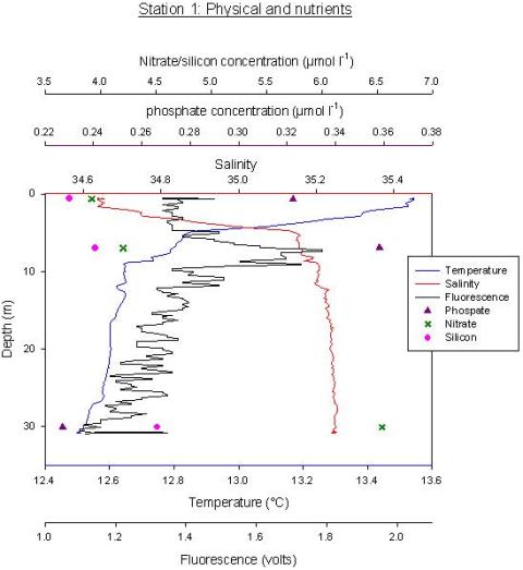
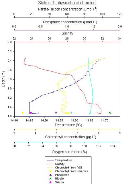
Fig 1.0: CTD Station 1

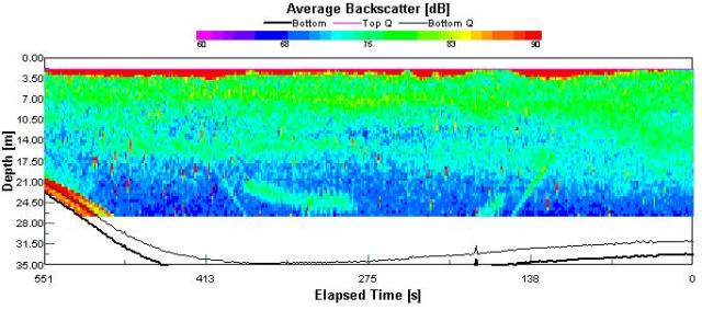
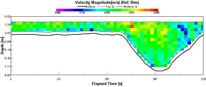
Fig 1.1: ADCP Station 1

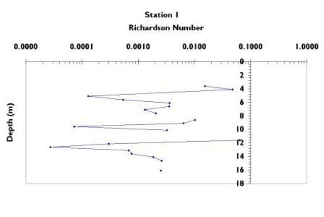
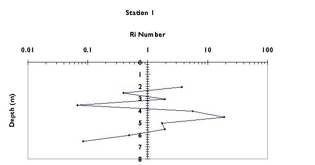
Fig 1.2: Ri Station 1

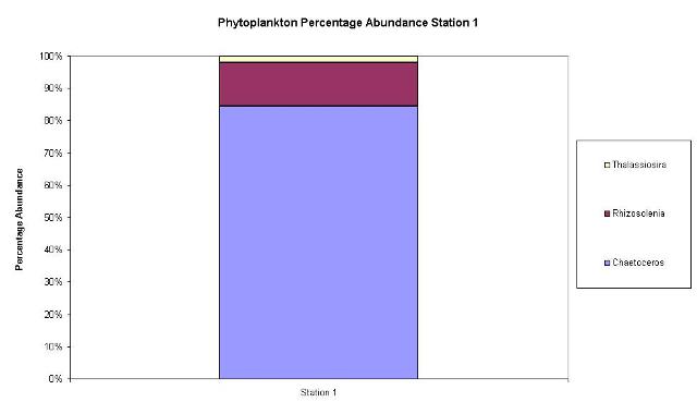
Fig 1.3: Phytoplankton Station 1 0m

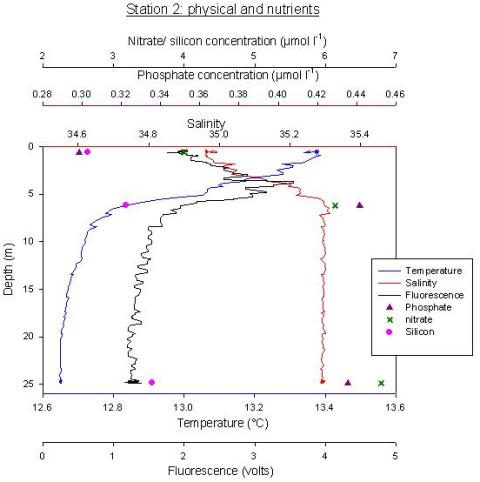
Fig 1.4: CTD Station 2

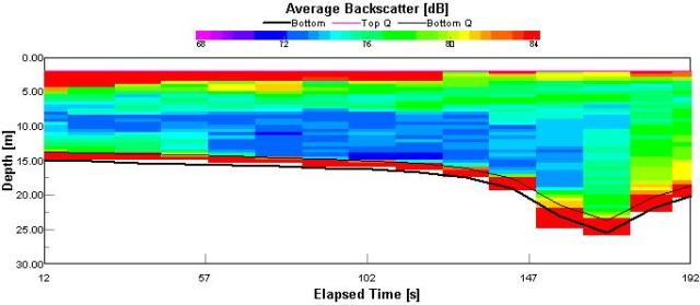
Fig 1.5: ADCP Station 2

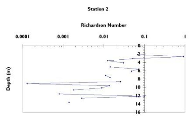
Fig 1.6: Ri Station 2

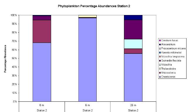
Fig 1.7: Phytoplankton St 2 0/6/25m

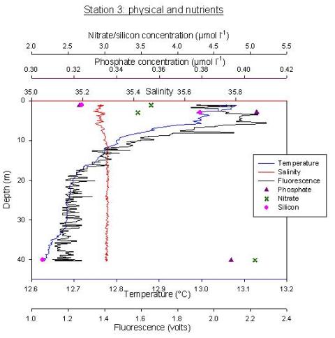
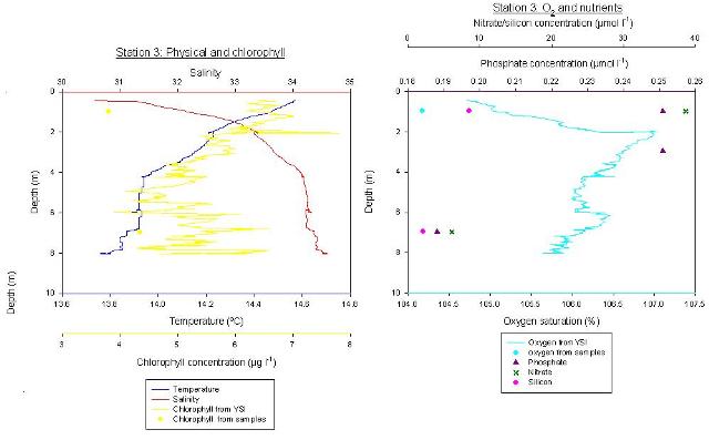
Fig 1.8: CTD Station 3

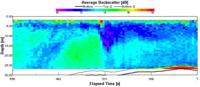
Fig 1.9: ADCP Station 3

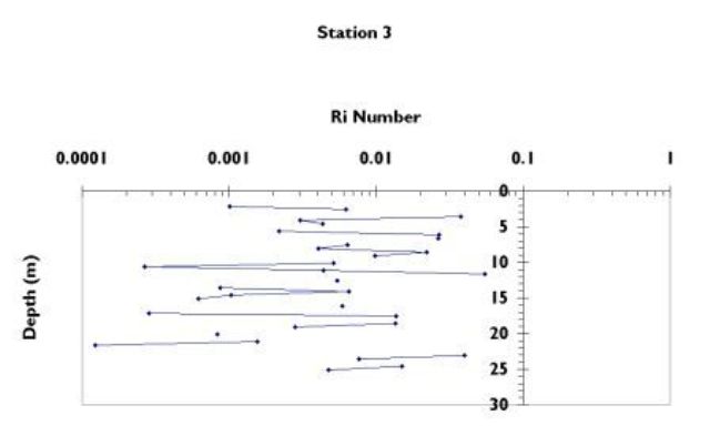
Fig 2.0: Ri Station 3

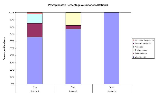
Fig 2.1: Phytoplankton St 3 0/3/14m

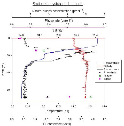
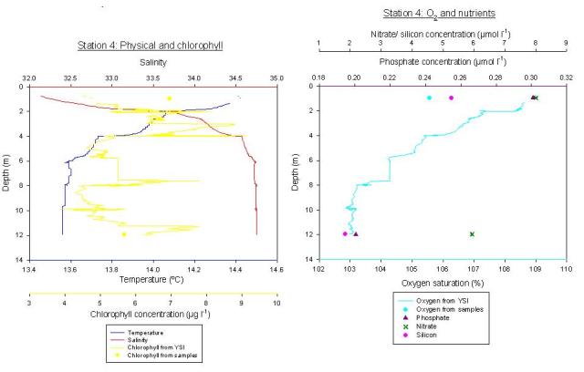
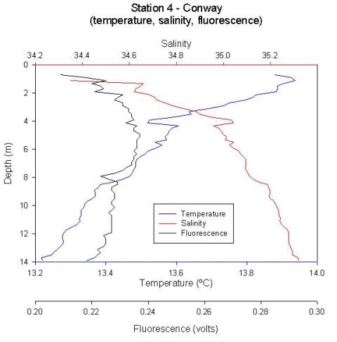
Fig 2.2: CTD Station 4

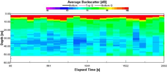
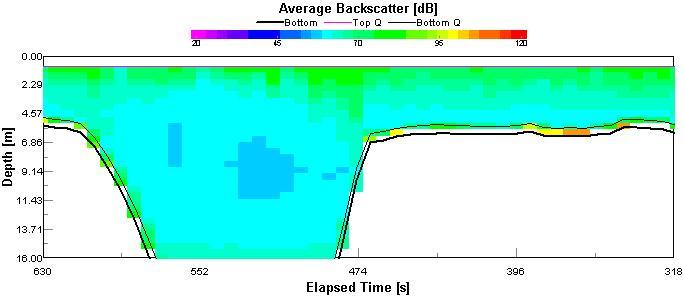
Fig 2.3: ADCP Station 4

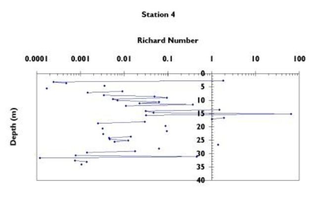
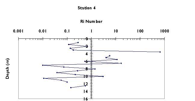
Fig 2.4: Ri Station 4

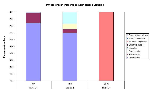
Fig 2.5: Phytoplankton St 4 0/14/68m

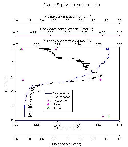
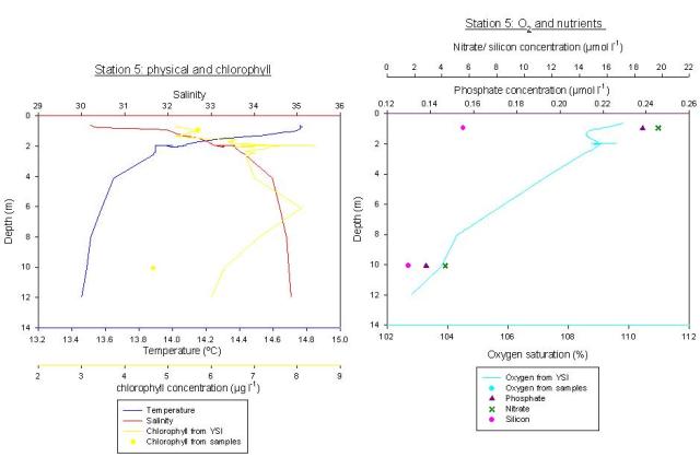
Fig 2.6: CTD Station 5

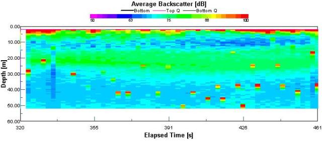
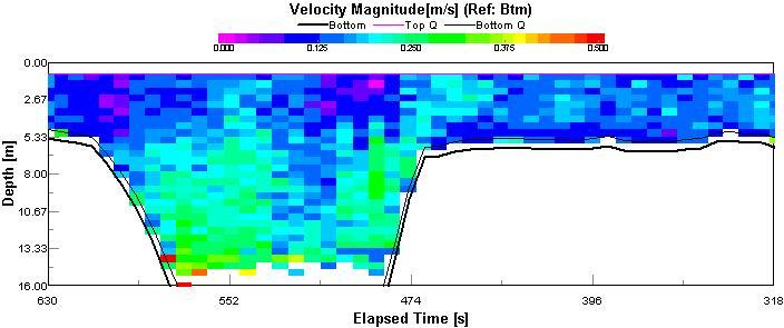
Fig 2.7: ADCP Station 5

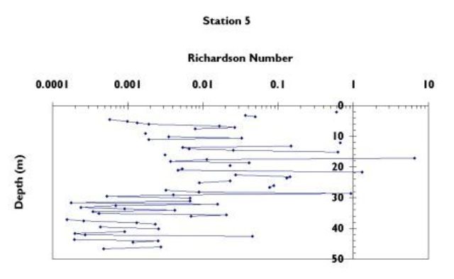
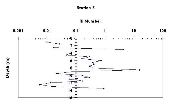
Fig 2.8: Ri Station 5

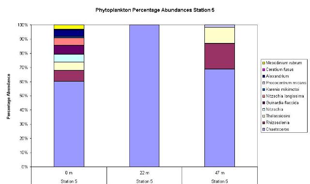
Fig 2.9: Phytoplankton St 5 0/22/47m

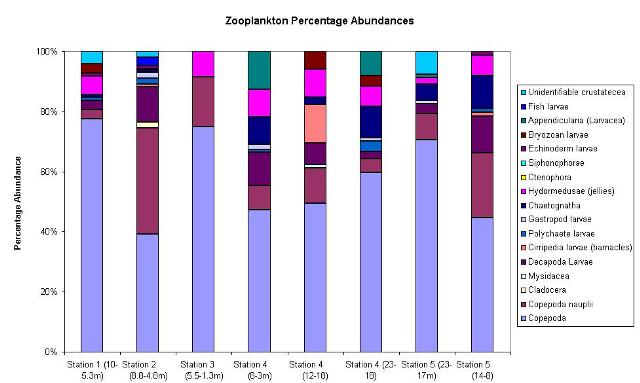
Fig 3.0: Zooplankton Stations 1-5

Method

From the entrance of Falmouth Harbour, Black Rock, it was planned to travel steadily offshore. Due to strong winds, it was advisable to carry out the investigation in the shelter of the headland. ADCP data was collected between stations and was monitored to look for any fronts, or other physical parameters. At 5 stations a CTD cast was completed and water samples were taken at the bottom of the cast, at the thermocline and at the surface in Niskin bottles. The samples were then split and preserved for later nutrient, chlorophyll, oxygen and phytoplankton analysis. A plankton net was deployed and the resulting sample preserved, and a Secchi disk was used to estimate the euphotic zone at each station. Station 2 was located near a front, so Station 3 was only 1 nautical mile south, aiming to sample the other side of the front. Station 4 was 5 nautical miles from station 3, to obtain samples from a range of offshore conditions.

The water samples were taken to the laboratory to be analyzed for taxonomic identification and abundance of zooplankton and phytoplankton species, nitrate, phosphate, silicate and chlorophyll.

Nitrate samples were analysed with the use of a spectrophotometer via the Flow Injection Technique as described in Determination of nitrate and nitrite in seawater by flow injection analysis, by Johnson and Petty, in Limnology and Oceanography 1983 (28, 1260-1266).  Each sample was passed through the spectrophotometer twice in order to increase accuracy and reliability.

Phosphate samples were analysed using the spectrophotometer method, discussed in A Manual of Chemical and Biological Methods for seawater analysis by Parsons and Lalli (1984). Replicates were taken to check the suitability of the method and the accuracy of the results.

Silicate samples were analysed in much the same way. Standards were produced with concentrations of 1.4, 2.8, 7.1, 14.2µmoles of silicon and their absorbance was measured. A calibration curve was produced and the silicon concentration from each sample was calculated from it.

Oxygen samples were analysed using a 665 Dosimat Titrator, using methods from A Manual of Chemical and Biological Methods for seawater analysis by Parsons and Lalli (1984).  Oxygen samples from the surface samples at stations 2 or 4 are not present as they were smashed due to the rough weather on the boat.  However, after analysis in the lab, it was found that the pipette used was calibrated inaccurately so the data cannot be included. 

Back to Top

Results

Station 1: Black Rock

The CTD data shows clear relationships between temperature, salinity and fluorescence. A significant thermocline of 0.9ºC is present at a depth of about 9m. There is also a small halocline in the top 7m with a change of 0.6, which implies that warmer and less saline river water overlies the cooler and denser seawater. This is an indication that riverine input is still significant at this location. The fluorescence shows a well defined chlorophyll maximum at approximately 7m, the same depth as the halocline. The values steadily increased from the surface (1.375) to the chlorophyll maximum (1.77), and then decreased gradually to the bottom, measuring 1.1 at 30m. The ADCP data taken is of the entire transect. It was taken at the same time as the CTD was deployed, which is why there are 2 thin diagonal lines of high backscatter in the profile between 17 and 24m depth. There is a large patch of high backscatter values in the surface 7m which may be attributed to the high plankton population caused by the favourable conditions and the lack of mixing due to the thermocline and halocline. There is another patch of high backscatter at about 14m depth, suggesting that it may be a zooplankton population feeding below the overlying phytoplankton population. The chlorophyll and phosphate trends contrast with the CTD data and what would be expected in the environment, except that the changes are small so they may be attributed to riverine input. Nitrate concentrations increase with depth because it is utilised nearer the surface by phytoplankton. Silicon increases with depth, which suggests it is being regenerated at depth from the earlier spring bloom. The phytoplankton was dominated by the diatom Chaetoceros; comprising about 85% of the total found. There were also small numbers of Rhizosolenia setigera and Thalassiosira. The dominant zooplankton was Copepod (80%), and small numbers of 8 other taxa were found. Nitrate, phosphate and silicon were all present at significant concentrations in the surface waters, therefore not limiting the bloom.

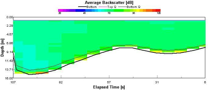
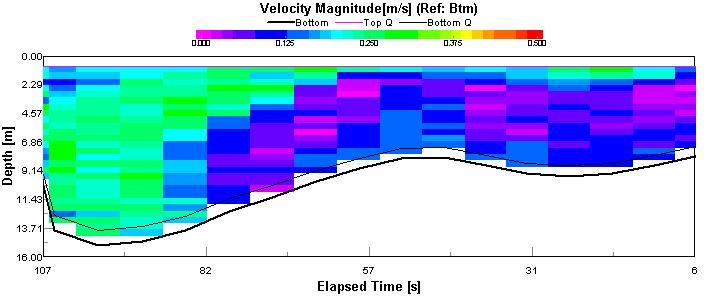
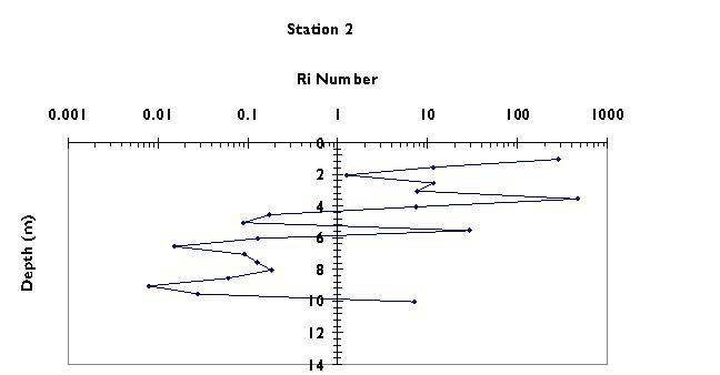
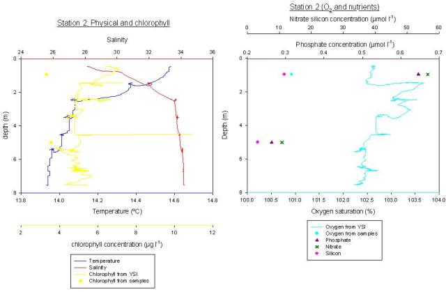
Station 2: 2 NM South of Black Rock

Temperature decreases with depth and a small thermocline of about 0.4ºC is present at 6m. There is a halocline of 0.35 to a depth of about 6m also, which suggests that there is still riverine influence, but not to the same extent as station 1, due to the fact that it is farther offshore. Fluorescence increased from the surface to the chlorophyll maximum at about 4m. This is shallower than station 1, which can be attributed to the reduced riverine input and the developing frontal conditions. The ADCP data indicated that there was a possible front developing, and temperature and salinity values reflect this when comparing the up and downcast, noting the variability between the two especially in the top 5m. The weather conditions lead to inevitable drifting, which could have effected the results of the up and downcasts, reducing the accuracy of the data. The ADCP transect between 147 and 192 seconds shows that there is a high amount of backscatter that spreads out towards the surface and is present at depth, suggesting that a front was developing here with high amounts of phytoplankton contained within it. Chlorophyll shows a similar profile to that at station 1. It decreases in the top 8m, which suggests that more water samples should have been taken, because of the developing front and the drift of the boat. The nutrients all increase with depth, suggesting they are being utilised at the surface by the plankton. Copepod and Copepod nauplii comprise the majority of zooplankton, about 75%. Many other species of nauplii were also found but in smaller numbers, with decapod larvae being slightly more significant. At all depths, Chaetoceros are the dominant phytoplankton, but particularly at 6m where they are approximately 95% of the population. In the surface waters, Rhizosolenia deliculata comprise a significant proportion whereas at 25m Guinardia flaccida and Nitzschia are present in high numbers.

Station 3: 3 NM South of Black Rock

The temperature decreases with depth until 18m, showing a thermocline of 0.35ºC. This is deeper than the previous stations but not stronger, probably due to the prolonged period of rainfall prior to sampling. A halocline of approximately 0.04 at a depth of about 10m shows that although very small, there is still a significant freshwater influence likely caused by excessive rainfall or the limit of the riverine input. This station was purposely close to the previous station so that the front could be investigated further. The fluorescence maximum of 2.25 at 6m is shallower than the thermocline and halocline. This indicates a large phytoplankton population. The ADCP shows that the boat had just travelled over the front by a clear line of low backscatter that shows the front pushing out from depth, towards the surface. Above this region and towards the left, there is a small area of higher backscatter which may represent a diatom bloom that occurs in frontal zones. There is also a large patch of backscatter towards the right of the front, which is more stratified and points to a possible dinoflagellate bloom. There is a large peak in chlorophyll at 3m, but the CTD profile suggested that more water samples would have placed the peak at 6m. Both phosphate and silicate increase to the chlorophyll maximum, which is unusual and is probably due to poor sampling or chemical analysis. Nitrate decreases in the top 3m due to utilisation by plankton, but increases to 40m. Station 3 is again dominated by Copepods (~75%), with Copepod nauplii and hydromedusae species also present. Chaetoceros dominated the phytoplankton counts at all depths. Rhizosolenia at Nitzschia were also present in the surface waters, and Thalassiosira and Rhizosolenia spp. at the chlorophyll maximum (3m), although in far smaller concentrations than Chaetoceros. Again, nutrient concentrations increased with depth but were not limiting.

Station 4: 10 NM South East of Black Rock

There is a strong thermocline of 2.1ºC at 25m, which is much deeper than the previous station, confirming the existence of a front by illustrating stratified conditions. Temperature clearly decreases with depth and salinity increases with a gradient of 0.15, showing a halocline. The halocline is stronger than that at the previous station which suggests it is caused by localised rainfall rather than riverine input. The ADCP data shows a typical profile through the water column, with high amounts of backscatter from the surface and at the thermocline from phytoplankton populations. There is less backscatter with depth as the phytoplankton populations decrease. Chlorophyll peaks at about 18m, which coincides with the peak in fluorescence, which is as expected. All the nutrient concentrations increase with depth, indicating utilisation by phytoplankton in the surface waters. At Station 4, all three zooplankton trawls found Copepods to be the main species present. In all three trawls many other taxa were found only in smaller numbers, many being larvae. Again, Chaetoceros were the dominant phytoplankton at the surface and the chlorophyll maxima, measuring 75% or more. However, Nitzschia longissima was the sole species found at 68m. At the surface, Rhizosolenia setigera and Prococentrum micans were present, but in the chlorophyll maximum many other species were present; including Nitzschia, Rhizosolenia spp. and Thalassiosira. Nitrate, phosphate and silicon surface concentrations were much less then at previous stations, although probably not limiting. The ADCP data shows a high backscatter in the surface waters indicating phytoplankton presence. The plankton counts reveal a greater number present than at other stations.

Station 5: 15 NM South East of Black Rock

At Station 5, a thermocline with a 2ºC change was present at about 26m, which is slightly deeper than the thermocline at station 4. There is a small halocline of about 0.1 to 9m. Fluorescence peaks at 3.5 at 19m which is quite high and similar to station 4. The ADCP data shows a large area of high backscatter between 15-25m depth below a smaller area of backscatter from the surface to 10m depth. It is likely that the deeper patch contains zooplankton feeding on the phytoplankton population in the shallower patch. Chlorophyll peaks at 1.5m which is quite shallow. It is likely that the thermocline at 26m hadn’t been detected in the chlorophyll samples. Phosphate and nitrate is depleted down to the thermocline because the phytoplankton population present. Silicate increases down to 22m, but loss of some of the data makes it difficult to analyse because the thermocline was so deep. The zooplankton is once more dominated by Copepods and Copepod nauplii at both depths trawled. There were also several other taxa present in smaller numbers. As before, Chaetoceros dominated the phytoplankton but the surface layers contained small numbers of many other taxa. The chlorophyll maximum was dominated by Chaetoceros but also contained Rhizosolenia species. The bottom plankton trawl also contained Rhizosolenia species as well as Thalassiosira and Prococentrum micans. Nitrate, Phosphate and Silicon surface concentrations were again depleted more so than station 4 but still did not reach zero values and so are probably not limiting.

Back to Top

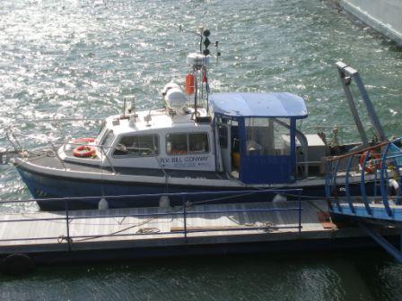
Introduction: Estuarine Processes

R.V. Bill Conway

Aim:

To collect data relevant to the biological, chemical, and physical aspects of the inland Falmouth estuary for an overall picture of the waterway.

Objectives: 

·  To sample water at the lowest salinity possible (i.e.; as far upstream as possible) and at the mouth of the estuary in order to obtain data over a wide salinity range.

·  To quantify any physical and chemical processes, and determine how they affect mixing and the distribution of nutrients.

·  To understand plankton community structure throughout the estuary at various depths.

Vessels:  

R.V. Bill Conway

7m Rigid Inflatable ‘Ocean Adventure’

Tides: HW:1156GMT 4.5m (neaps)

 Weather Forecast: 7/8 Cloud cover. Scattered showers. North Westerly 3-4.

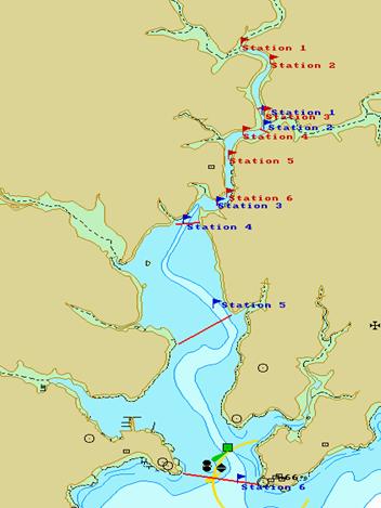
A chart showing the location of the RIB sampling stations (in red) and the Bill Conway sampling stations (in blue). The ADCP transects completed by the Bill Conway are shown as red lines.

Back to Top

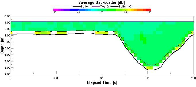
Fig 3.1:ADCP Backscatter Station 1

Fig 3.2: ADCP Velocity Station 1

Fig 3.3: Ri Plot Station 1

Fig 3.4: YSI Rib Station 1

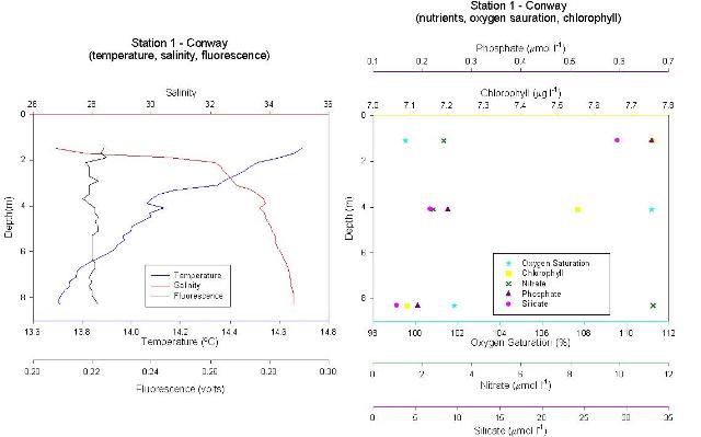
Fig 3.5: CTD Station 1 Conway

Fig 3.6: ADCP Backscatter Station 2

Fig 3.7: ADCP Velocity Station 2

Fig 3.8: Ri Plot Station 2

Fig 3.9: YSI Rib Station 2

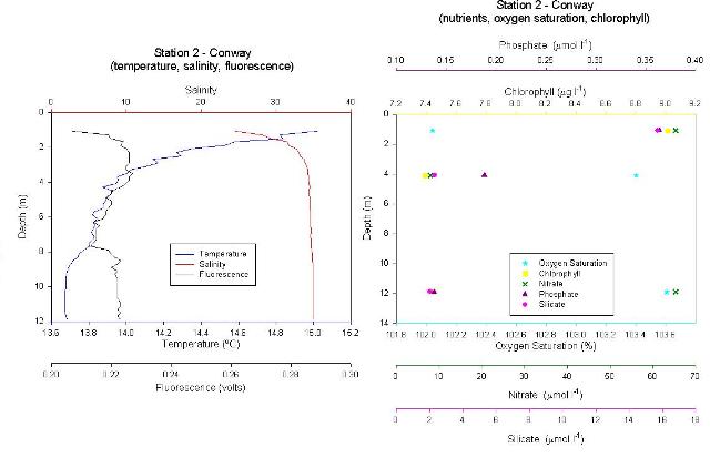
Fig 4.0: CTD Conway Station 2

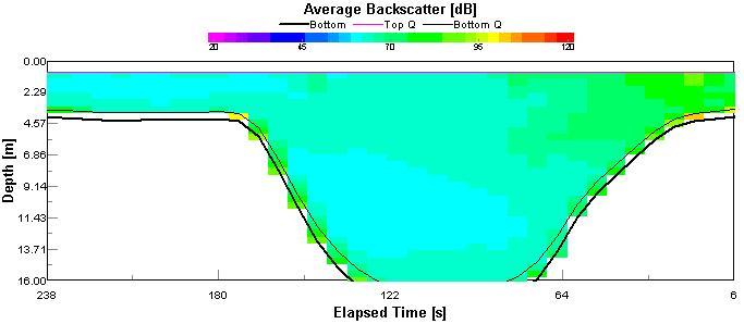
Fig 4.1: ADCP Backscatter Station 3

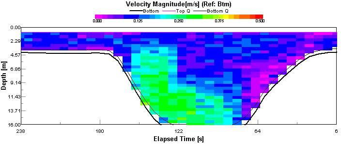
Fig 4.2: ADCP Velocity Station 3

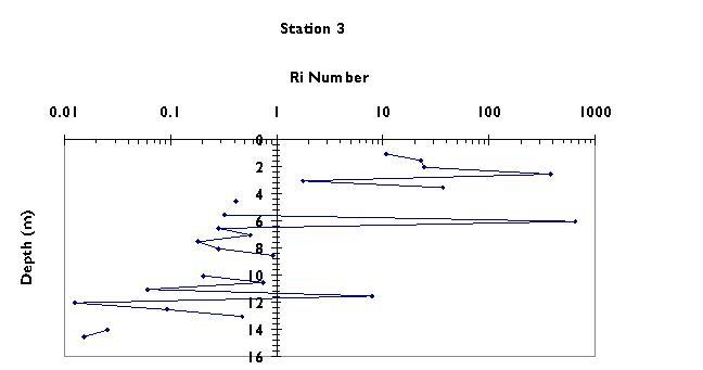
Fig 4.3: Ri Plot Station 3

Fig 4.4: YSI Rib Station 3

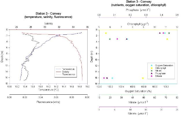
Fig 4.5: CTD Conway Station 3

Fig 4.6: ADCP Backscatter Station 4

Fig 4.7: ADCP Velocity Station 4

Fig 4.8: Ri Plot Station 4

Fig 4.9: YSI Rib Station 4

Fig 5.0: CTD Conway Station 4

Fig 5.1: ADCP Backscatter station 5

Fig 5.2: ADCP Velocity station 5

Fig 5.3: Ri Plot Station 5

Fig 5.4: YSI Rib Station 5

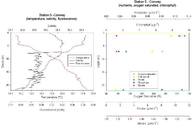
Fig 5.5: CTD Conway Station 5

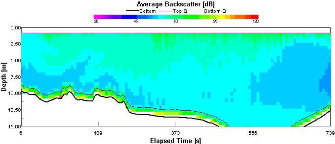
Fig 5.6: ADCP Backscatter station 6

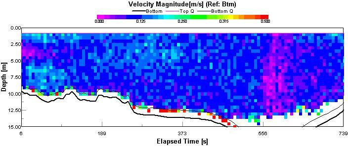
Fig 5.7: ADCP Velocity station 6

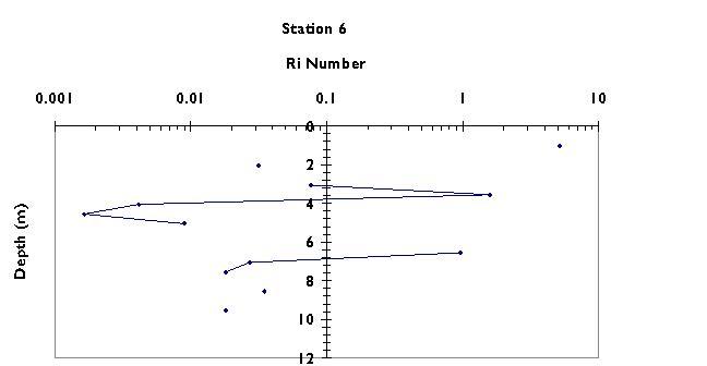
Fig 5.8: Ri Plot Station 6

Fig 5.9: YSI Rib Station 6

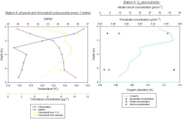
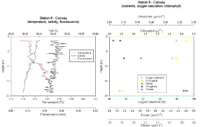
Fig 6.0: CTD Conway Station 6

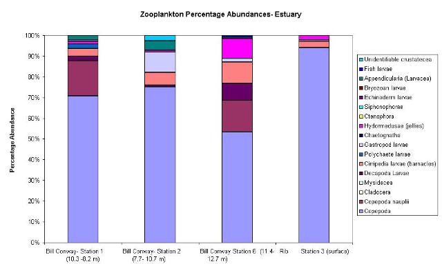
Fig 6.1: Zooplankton All Stations

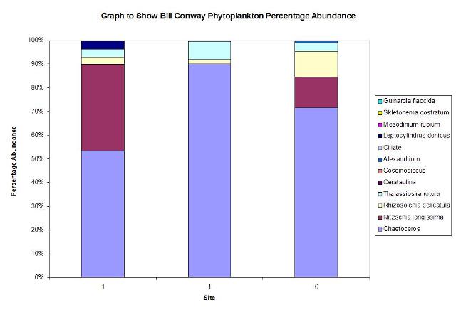
Fig 6.2: Phytoplankton Species, Bill Conway Stations

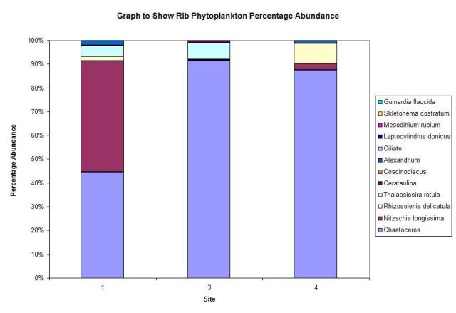
Fig 6.3: Phytoplankton Species, RIB Stations

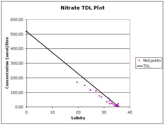
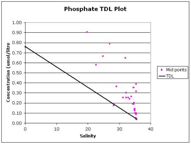
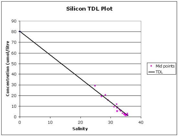
Figs 6.4-6.6: TDL plots for Nitrate, Phophate and Silicon

 Method

Aboard the R.V. Conway six stations were sampled in the Fal Estuary beginning farthest upstream, due to tides and the weather. Interesting surface features such as scum and a colour gradient on the surface indicated a front, and this was reflected in a sharp change in surface salinity being monitored by the deck pump system. At certain points throughout the estuary an ADCP transect was completed. The CTD was then deployed, and a Secchi disk was used to estimate the euphotic zone. At stations 1 and 6 a plankton net was deployed and towed at 2.5 knots for 2.5 minutes.

The upper parts of the estuary were investigated by use of the RIB, allowing lower salinity samples to be collected. Six stations were located, at specific points moving down the estuary towards the sea and incoming tide. At each station a multi parameter YSI probe was deployed in order to obtain a vertical profile of the water column. Water samples were taken at the surface and at depth where possible, although the space onboard the RIB limited the number of sampling bottles allowed. After station 3, a dragging plankton net was deployed for a period of 5 minutes, with zooplankton samples collected and preserved.

Station Information: Estuarine practical 10/07/07,R.V Ocean Adventure:

Station 1: Malpas   50’14.692N   005’01.374W   0912GMT

Station 2: 50’14.446N   005.00.842W   1002GMT

Station 3: Ruan Pontoon 50’13.713N   005’00.948W   1047GMT

Station 4: Smugglers Cottage 50’13.434N   005’01.342W   1120GMT

Station 5: 50’13.098N   005’01.342W   1220GMT

Station 6: 50’12.556N   005’01.674W   1249GMT

Equipment available aboard the RIB:

• YSI multi parameter probe

• 1 litre Niskin bottle

• Glass and plastic sampling bottles (for chemical and biological samples)

• Towing plankton net (200µM Mesh size, 59cm diameter)

• Secchi disk

Station Information: R.V. Bill Conway: (horizontal transects taken at each station).                   

Station 1 :

Start: 50’13.737N  005’00.993W 0940 GMT

End:   50’13.807N  005’00.987W 0942 GMT

Station 2: 

Start: 50’13.522N  005’00.963W 0953 GMT

End:   50’13.537N  005’00.908W 0955 GMT

Station 3: 

Start: 50’12.435N  005’01.826W 1035 GMT       

End:   50’12.425N  005’01.732W 1036 GMT

Station 4: 

Start: 50’12.162N  005’02.456W 1118 GMT

End:   50’12.138N  005’02.370W 1123 GMT

Station 5:

Start: 50’10.969N  005’01.896W 1140 GMT

End:   50’10.932N  005’01.799W 1151 GMT

Station 6:

Start: 50’08.478N  005’01.444W 1240 GMT

End:   50’08.406N  005’01.343W 1253 GMT

Equipment available on the R.V Conway:

• Closing plankton net (200μM mesh size, 59cm diameter).

• Secchi disk.

• Glass and plastic sampling bottles (chemical and biological samples).

• ADCP

• CTD array with 6 1 litre Niskin bottles attached, T/S probe, fluorometer and transmissometer.

Back to Top

Results

The following section contains the data collected from both the rib and Bill Conway. The data from the rib is analysed first.

For 5 stations sampled on the rib, the YSI probe was used, but for station 6, the data had to be collected manually because the YSI probe ran out of memory. The YSI probe has constraints, of which some are shown on the graphs. The first being that the YSI probe only has a small resolution so it is not precise enough to use exact values, or to make detailed conclusions. However, we can draw relative conclusions. For more detail, the probe needs to be calibrated with samples analysed in the lab from all the groups to make it more accurate. This can be done for both chlorophyll and oxygen saturation, as on the graphs the YSI data appears to be quite different to our collected sample. However, for chlorophyll, this variation could be caused by the phytoplankton species, which may have differences in the chlorophyll types, amounts etc. which isn’t picked up by the YSI probe or poor sampling.

Station 1:

Temperature decreases from 14.7°C to 14.45°C, over a depth of 1m, and salinity shows a large change from 23 to 32 over the same depth. The water was too shallow for a thermocline or halocline to develop, but the large change in salinity reflects the freshwater dilution of the surface water, which overlies the salty water from the incoming tide. The oxygen saturation remains relatively constant with depth at about 100.05%, suggesting that the water column is almost in equilibrium with the atmosphere, although these readings from the YSI probe are highly suspect, and differ from the collected water sample by 2%. Chlorophyll decreases from 8.5 – 5.5µg l^-1 until 0.7m, after which it stops decreasing. This is also highly suspect and varies from the water sample value by 2.5µg l^-1 for the reasons mentioned previously. There was only one sample taken at this station because it was too shallow, so nutrients cannot be analysed with respect to depth, in this case. The phytoplankton sample shows that the water at 1.5m was evenly dominated by the diatoms Chaetoceros and Nitzschia longissima, with minor populations of dinoflagellate Alexandrium. This is unusual for the time of year, because a dinoflagellate bloom should be more abundant in the summer, but because of the poor weather conditions, i.e. lack of insolation, high precipitation and strong winds, the diatom population thrives instead.

Station 2:

Temperature generally decreases with depth, sharply until 2m, from 14.6 to 14.1°C after which, there is little change. This is perhaps a small thermocline. Salinity changes from 28 to 34 over a depth of 7m, corresponding to the temperature change. After 2m, salinity remains relatively constant. Chlorophyll shows a very spiky profile, which may be attributed to poor YSI calibration, with a large anomaly at 4.5m where it reaches 11µg l^-1. Generally, most values lie within 4 to 7µg l^-1. There is a slight increase in chlorophyll at the surface but it is not immediately obvious.  Our water samples, show lower values than the YSI probe again, with a difference of 4µg l^-1 at a depth of 1m. Oxygen saturation is also very spiky and is not representative of the water column due to poor resolution of the YSI probe. Nitrate decreases from 57 to 13µmol l^-1 over a 4m depth. Phosphate decreases from 0.65 to 0.26µmol l^-1 over 4m depth. Silicate decreases from 11 to 3µmol l^-1 over 4m. These nutrients show a decrease in concentration with depth, because they reflect the riverine input of fresher water at the surface, which typically contains higher concentrations of the nutrients compared to seawater. This is true for stations 3, 4 and 5 also. There was no phytoplankton sample for this station.

 Station 3:

A temperature change can be seen from 14.7 to 13.8°C over a depth of about 8m. It is a gradual change showing no obvious thermocline. Salinity changes from 26.5 to 34.3 over a depth of 8m. A slight halocline is present to a depth of about 4m. Chlorophyll shows a very spiky profile through the water but there is a general decrease from 7to 5µg l^-1 over a depth of 8m. The chlorophyll samples show an increase with depth from 4 to 4.5µg l^-1 over a depth of 6m perhaps due to surface mixing or the very high amount of insolation from the few days before sampling. In the top 1m, the water column is over saturated with respect to oxygen. There is a peak in saturation at 2m, after which it decreases. It is likely that oxygen saturation is higher in the surface waters because of entrainment from the atmosphere caused by mixing. Oxygen saturation decreases with depth, because there is less mixing deeper in the water column, and oxygen is also utilised by organisms in the water column. This is also the case for stations 4, 5 and 6. Nitrate decreases from 38 to 7µmol l^-1 over a depth of 6m. Phosphate decreases from 0.25 to 19µmol l^-1 also over 6m. Silicate decreases from 9 to 2µmol l^-1 over 6m. Phytoplankton at a depth of 1m at this station was mainly the diatom Chaetoceros, whilst the zooplankton was dominated by copepods.

 Station 4:

Temperature decreases from 14.4to 13.6°C in the top 6m and remains relatively the same after 6m, indicating a possible thermocline. Salinity increases from about 32.2 to 34.6 at 5m, which is a possible halocline. Chlorophyll shows a very spiky profile with values between 4-8µg l^-1, but no obvious change with depth. The chlorophyll samples decrease from about 7 to 5.5µg l^-1 over an 11m depth. The oxygen saturation profile shows a decrease gradually with depth from about 109 to 103%. At a depth of 1m, our sample showed that the water was oversaturated with respect to oxygen at 105.5%. Nitrate decreased from 8-6µmol l^-1 over a depth of 11m, whilst phosphate decreased from 0.3 to 0.2µmol l^-1 over 11m depth. Silicate decreased from 5.3 to 1.9µmol l^-1 over 11m depth. The phytoplankton sample taken at 1m was dominated by Chaetoceros.

 Station 5:

Temperature decreases from 14.8 to 13.4°C over a depth of 11m, showing a possible thermocline. Salinity increases from about 30.2 to 34.9 over a depth of 11m, showing a possible halocline. Chlorophyll from the YSI increases until 6m, but then greatly decreases between 6-12m. The samples show a decrease from 6 to 4.5µg l-1 over 9m. Oxygen saturation decreases from 110 to 103% over a depth of 11m. Nitrate decreases from 20 to 4µmol l-1 over 9m, whilst phosphate decreases from 0.24 to 0.14µmol l-1 over the same depth. Silicate also decreases from 5.5 to 1.5µmol l-1 over 9m.

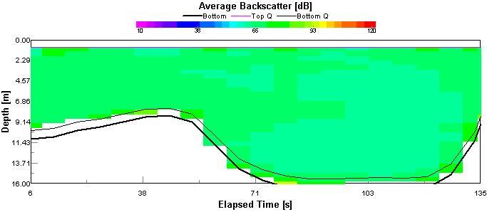
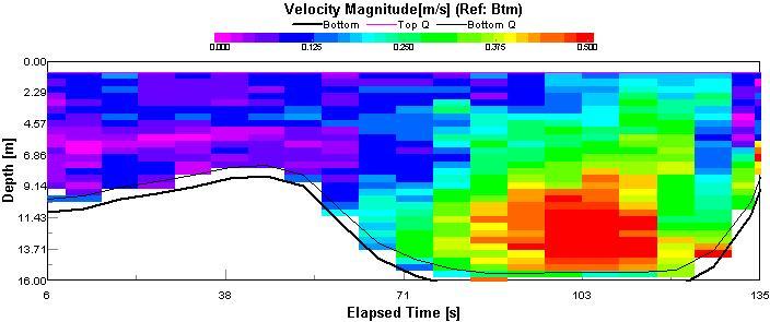
Station 6:

Temperature decrease from 14.7 to 13.6°C over a 7m depth, which is a possible thermocline. Salinity increases from 30 to 36 over 7m. Chlorophyll increases from 5 to 10µg l^-1 in the top 3m, but then decreases from 10-5µg l^-1 from 3-7m. The chlorophyll sample at 6m is 8µg l^-1. The oxygen saturation increases from 111 to 113% in the top 2m, then decreases to 106 from 2 to 7m. Nitrate decreases from 34 to 4µmol l^-1 over 5m. Silicate decreases from 10-3µmol l^-1 over 5m. Phosphate increases from 0.25-0.35µmol l^-1 over 6m, which is different from the rest of the nutrients. This may be because of industrial input.

 Bill Conway Results

The zooplankton communities that were collected from 1m and 4m at station 1 and 1m at station 6, show a definite pattern.  Copepods were the most dominant throughout, followed by nauplii.  Cirripedia and Hydromedusae species were also present in high numbers.  There appears to be a trend of greater copepod abundance nearer the mouth, however more data would be needed to test this.  

Station 1

The temperature at station 1 decreased steadily with depth from 0 to 8m from 14.8^oC to 13.7^oC.  There was a decrease in salinity with depth from 27psu at the surface, through a halocline at 2m of 7psu due to the less dense riverine input, this is also shown in the other station.  Below this salinity was relatively constant at 34psu.  Fluorescence was very low at the surface and increasing there after from 0.14 to 0.22 volts in the surface 2m and remaining constant with depth.  Phosphate and silicate have a maximum at the surface and decrease sharply to 4m, from 0.7 to 0.25 mmol l^-1 and 28 to 7mmol l^-1 respectively, then decrease steadily from 4 to 8m.  This is due to nutrient input via the riverine flow.  Nitrate is constant at 3mmol l^-1 over the first 4m, then increases to 11mmol l^-1 at depth.  Chlorophyll decreases steadily with depth from 7.75 to 7.10 mg l^-1.  The oxygen percentage saturation at station 1 increases over the first 4m from 99 to 111% then decreases to 102% at a depth of 8m.  The ADCP data showed the highest velocities above the channel of about 0.475m/s and the average fast flow was approximately 0.375m/s.   The backscatter showed that at the fastest flow there was the least backscatter, suggesting less phytoplankton concentration.  In areas of slower flow, there was an average backscatter value of approximately 70 decibels.  Phytoplankton samples taken from this station were taken either side of a front, the first sample was taken from the upstream side of the front and the second taken from the downstream side of the front. From the first water sample the dominant species of phytoplankton are Chaetoceros and Nitzschia Longissima both having a percentage abundance of 53% and 37% respectively. Thalassiosira Rotula was identified in the sample and made up 3% of the total phytoplankton count, Leptocylindrus donicus and  Rhizosolenia delicatula have also been identified and represent 4% and 3% respectively.

The second sample at this station shows Chaetoceros dominating at about 90% and Thalassiosira Rotula then at about 8%. Rhizosolenia delicatula is also present but at very low percentage (2%). 

Station 2 

The temperature profile at station 2 has a sharp decrease from the surface to 3m of 1.3 ^oC and is constant there after at 13.7 ^oC.  Salinity increases from the surface down to 3m from 26psu to 35psu, and below that it remains stable.  Fluorescence increases from 0.19 to 0.22 volts in the first 2m and is constant with depth below this.  The phosphate plot is similar to that of station 1, decreasing from 0.36 to 0.19mmol l^-1 in the first 3m and decreasing more slowly after to 0.15mmol l^-1 t o 12m.  Silicate has a maximum at the surface of 15mmol l^-1 decreasing to 2mmol l^-1 at 4m and constant there after.  Nitrate also has a maximum at the surface of 66mmol l^-1 and decreases sharply to 8mmol l^-1 at 4m.  It then remains constant to a depth of 12m.  Chlorophyll decreased from 9 to 7.4mg l^-1 in the first 4m and the sample taken at depth was lost so the data is missing.  Oxygen percentage saturation increases with depth from the surface minimum of 102% to 103.3% at 4m and then 103.6% to depth.  The fastest flow, at approximately 0.3m/s, was above the channel and at the outside of the bend due to flow dynamics.  The slowest flow was on the opposite side of the transect, reaching values close to 0m/s.  Again, the least backscatter (60 decibels) was recorded at the fastest flow point, while in areas of slower flow the average backscatter was approximately 90 decibels.

Station 3

Temperature decreases over 17m steadily from 14.9 to 13.3 ^oC.  There is a salinity increase in the first 4m of 7psu, from 27 to 34psu and is stable down to 17m.  Fluorescence increases from 0.14 to 0.23 volts in the first 2m, and then remains constant with depth.  Phosphate decreases sharply from 0.4 to 0.2mmol l^-1 in the upper 3m then decreases to 0.1mmol l^-1 at depth. Silicate has a maximum at the surface of 22mmol l^-1 decreasing to 7mmol l^-1 at 3m and then decreasing to 2mmol l^-1 at 16m.  Nitrate decreases from the surface to 3m, from 75 to 20mmol l^-1 and is constant with depth there after.  Chlorophyll increases from the surface to 3m from 6 to 11mg l^-1 then decreases to 9mg l^-1 to depth.  The oxygen percentage saturation showed an overall decrease. The maximum surface value of 103.2% decreases to 102.5% at 3m and then to 102.2% at depth.  Very high velocities (approximately 0.5m/s) were found at the bottom of the mid channel, reducing to values of around 0.375m/s, and reaching almost 0m/s at the inside of the bend and the shallow areas.  The backscatter was again low, around 50 decibels, in areas of high water velocity, and high, 70 decibels where the water velocity was higher.  

Station 4

Water samples were not taken at station 4, but profiles of temperature salinity and fluorescence were recorded on the CTD.

The profile reveals temperature decreasing with depth (from 13.9 – 13.2°C) while salinity increased with depth over the 14m. A halocline was identified between 2-4m (34-36 arb units). Fluorescence increases to 0.235 V at 5m from surface value of 0.222 V, this then decreases to 0.217 V at a depth of 14m.  The channel at site 4 is divided, with close to zero flow on the right side and fast, 0.3m/s, on the left.  The backscatter was lowest in high water, and highest in the slow water on the right side. 

Station 5

Analysis of the results at station 5 yielded the following phenomena: temperature decreased uniformly with depth (13.8 to 13.2°C) between 1 and 22m whilst salinity increased with depth producing an almost mirror image of temperature and salinity on this profile.

A halocline has been identified in the salinity profile between 4m and 7m with a change in salinity values from 34.75 to 35.0 arb units over the 3 meters.

The readings for fluorescence at 7m suddenly dropped from 0.24 V to 0.18V (this occurred within 1m) and remain reasonably constant down the water column at 0.18 V.

Over the 21 meters from which the water samples were taken, Chlorophyll, Nitrate and Oxygen all decrease with depth, values (8.9 - 5.7µmol/l), (11.5 – 2.8µmol/l at 6m then constant from then on to 22m), (107 – 97.5%) respectively. Silicon is constant from surface to 7m with values 1.27µmol/l, and then increases to a value of 1.57µmol/l at 22m.  The slowest water (0.125) was on the surface with the fastest water moving down into the channel with a maximum of 0.375m/s.  The lowest backscatter, 50 decibels was mid channel, with 80 decibels the highest backscatter at the surface.

Phytoplankton samples taken from this station were taken either side of a front, the first sample was taken from the upstream side of the front and the second taken from the downstream side of the front. From the first water sample the dominant species of phytoplankton are Chaetoceros and Nitzschia Longissima both having a percentage abundance of 53% and 37% respectively. Thalassiosira Rotula was identified in the sample and made up 3% of the total phytoplankton count, Leptocylindrus donicus and  Rhizosolenia delicatula have also been identified and represent 4% and 3% respectively.The second sample at this station shows Chaetoceros dominating at about 90% and Thalassiosira Rotula then at about 8%. Rhizosolenia delicatula is also present but at very low percentage (2%).

Station 6

The temperature profile at this station reveals lower temperature values than previous stations, a very small decrease in temperature (0.2°C) from surface waters to depths of 18m occurs producing quite a uniform profile with a temperature change from 13.2 - 13°C.

A possible halocline was observed around 7m with values of 35.37 to 35.42 at 12m. Fluorescence was constant throughout the water column with a value of 17 V there is some variance in the profile but the fluorescence tends to remain around 17 V. Silicon, Nitrate and Phosphate increase with depth over the 17m sampled with values (1.65 – 2.9µmol/l), (3.1 – 4.9µmol/l) and (0.09 – 0.31µmol/l) respectively.

Chlorophyll decreases with depth from 5.2 – 2.7g/l from surface to 18m respectively. Oxygen also decreases with depth with saturation percentages of 98% down to 91%.  At this station the tide was slack because it was high tide, therefore the flow was slow throughout, however the slowest flow was over the channel.  The backscatter was highest on the surface on the surface at about 85 decibels, and lowest on the extreme left and right at approximately 55 decibels.  Phytoplankton at station six are split into 4 different species present. Chaetoceros are the dominant species with a percentage abundance of 70%, Nitzschia Longissima are the next most abundant species with 15%, Rhizosolenia delicatula 12% and Thalassiosira rotula 3%. Alexandrium sp. were present at very low concentrations <1%.

Secchi Disc Results 

R.I.B 

 R.V Bill Conway 

The secchi depths show that the euphotic zone of the estuary increases in a general trend moving seaward. This is probably due to a decrease in riverine inputs such as sediment load which settles out of the water column through the course of the estuary.

Summary

Although, temperature varies with depth, there isn’t much change with respect to the location of the stations. Salinity generally increases further away from the head of the estuary, which is as expected, and the salinity changes with depth indicate that a salt wedge structure is possibly present. It is difficult to make comparisons between the stations sampled because of the YSI calibration, and the sampled chlorophyll values are not that variable either. It appears as though oxygen saturation increases further from the head of the estuary, although because the YSI probe needs calibrating, a valid assumption cannot be made. Nutrient concentrations are highest at the head of the estuary which is as expected because of high concentrations in the run off into the river leading to the estuary. It is difficult to make comparisons between the phytoplankton and zooplankton samples at each station because of limitations in sampling equipment available at the time.

 Back to Top

Introduction: Geophysical Processes

M.V. Grey Bear

Friday 6^th July: P.S.O: Lizzy McMichael

Aim: To investigate the seabed surface type adjacent to the mouth of the Helford River Estuary and Falmouth Bay. To identify sediment boundaries and interesting features on the seafloor i.e. bed forms.

Vessel: MV Grey Bear, a 50’ landing craft.

Tides:

Weather Conditions: Dry and bright. 3/8 Cloud cover. Wind: westerly, 14 knots decreasing to 13.  No rain.

Transect locations

 Figure 6.7: A map showing the location of transect lines.

Back to Top

Method

In order to survey the seabed offshore from the Helford river estuary, specific transects were followed (see figure 6.7) using the MV 'Grey Bear'. Two side scan sonar, mounted either side of a 'fish' was towed behind the vessel, and the resulting images were printed out using a thermal recorder. A total of 6 North-South sidescan sonar transects were run South of Falmouth bay immediately East of the mouth of the Helford River Estuary (see map), and were each around 2km long.  The sonar results were used to locate specific positions of interest along each transect in which grab samples could be collected using a Van Veen Grab.  Five sites of interest were sampled which allowed the Sidescan traces to be calibrated, and also basic taxonomic identification of the benthos to be conducted.

Geophysical equipment on board the 'Grey Bear'

On board the Grey Bear, the farthest offshore transects were allocated in order to take advantage of the first day of calm weather conditions. The survey began at the north point of the farthest offshore transect and worked our way west through six consecutive north-south transects.  As the course of the transects were followed, three group members were in the wheelhouse with the skipper recording latitude, longitude, eastings, northings, and standard AST time at one minute intervals.  Two other group members were below with the side scan sonar display and printer, also noting the above variables as well as watching for interesting features appearing on the display.  When anything signifying a boundary in sediment appeared, the location would be marked on the print out. Later, the AST times on the profile could be matched up with the recorded latitude and longitude, in order to obtain exact positioning.  The exact positioning of the grab sites were entered into a G.P.S system, the locations revisited and grabs taken.

Analysis of the Van Veen Grab samples, involved rinsing the sediment through two mesh sieves of varying sizes in order to determine the general grain size, approximate percentages of grain type present and other physical properties. Any biology present was identified and photographed.

Back to Top

Results

Figure 6.8: A plot of the boundaries between seabed surface types, drawn from analyzing the side scan profile. Blue represents bed rock, purple represents coarse grained sediment, and pink represents fine grained sediment.

Analysis of the side scan sonar profile revealed 3 sediment boundaries that spanned the width of our survey site.  There were also three sediment patches which were either complete isolated areas or spanned part of the survey width.  Figure 2 shows the position of the boundaries and patches.  Although the weather was calm some noise from wave action was seen on the traces which had to be recognised and disregarded. Exposed rocky outcrops were apparent.  Between them are channels of coarse sediment and both are aligned perpendicular to the mouth of the estuary.  Interesting features included an anchor drag: located at 50 ˚06.2 N, 5˚ 03.6 W at 11:17:34 A.S.T.  Calculations from the print out found the feature to be  0.76m deep and the depth of the lip from the anchor to be 0.36m.  Mega ripples were identified along boundary 3: they were found to be sinuous in phase with a height greater than ten centimetres (24 – 43 cm) and length greater than twenty centimetres.

Back to Top

Discussion

Analysing the print out tracks of the Grey Bear through the transects revealed outstanding features which can be identified.  There are exposed rocky outcrops between which are channels of course sediment both aligned perpendicular to the mouth of the estuary.  The sonar indicated variations in seabed surface type which was then confirmed by an analysis of the grabs.  These analyses showed varying sediment and biota types helping to piece together an overall picture of the seabed.  At certain points within the channels of coarse sediment, mega ripples were identified and measured.  These mega ripples are sinuous in phase with a height greater than ten centimetres (24 – 43 cm) and length greater than twenty centimetres.  This shows that the flow through these channels must be greater than twenty centimetres per second.  Also noted was that the wave heights increased towards the shore, nearly doubling in height across the surveyed area.

Back to Top

Conclusion

The two weeks spent in Falmouth have allowed a large amount of information to be collected regarding the physical, biological, chemical and geophysical environments both within the Estuary and Offshore. As well as considering these aspects individually, it is important to understand how these factors influence and affect each other.

Defining the structure of the Fal Estuary was difficult. In July, a clear halocline structure is expected, with the overall classification being a salt wedge. However, this investigation has suggested that the Fal's structure in July 2007 is showing partially mixed characteristics. For example at several locations temperature and salinity varied little with depth. The phytoplankton succession was in an earlier stage than in 2006, with diatoms dominating the waters rather than dinoflagellates which would be expected at this time of year. These unusual findings may be attributed to above average precipitation during late May and June (June was the wettest month on record). This would have increased the riverine input into the Fal Estuary, and poor weather (e.g: strong winds and reduced insolation due to heavy cloud cover) leads to increased mixing and may delay the phytoplankton bloom.

These weather conditions and increased river discharge have also had an effect on the offshore environment, pushing the seasonal thermocline front further offshore than in the past. The water column near shore was generally well mixed with respect to both temperature and salinity; the thermoclines seen in the profiles were weak. The small haloclines detected could be attributed to larger than normal estuarine freshwater fluxes. This being said, the water column offshore is more stratified and a stronger thermocline can be seen in stations 4 and 5 offshore. Offshore chlorophyll peaks occured at the depth of the thermocline, deepening as the euphotic zone deepens further offshore.

Back to Top