|
|
|
|
|
|
|
|
|
|
 |
Here lies the account of nine intrepid students on an
oceanographic adventure during two weeks in July 2006.
|
 |
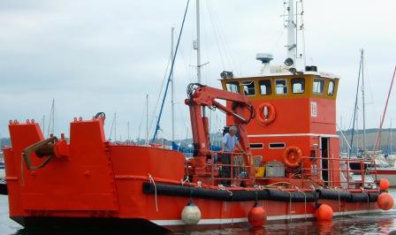
MV Grey Bear |
RV Bill Conway |
|
 |
 |
|
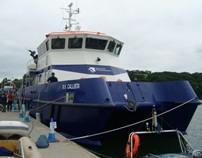
RV Callista |
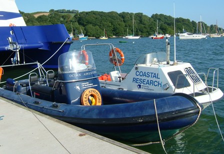
RV Ocean AdventureRV Coastal Research |
Click the photo's below to enlarge |
||||||||
 |
 |
 |
 |
 |
 |
 |
 |
 |
RobAka "the boss" |
TomAka "Fishwife" |
JimAka "The Leadloader" |
AndyAka "Chief Weasel" |
CharlieAka "The Artist" |
HelenAka "Maefanwey" |
LauraAka "Data Minx" |
SamAka "Mummy Logbook" |
NickAka "Chart-Master" |
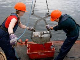
Sidescan sonar survey
Transects6 latitudinal transects were surveyed in order to obtain an overview of the sediment structures. Grab sites were then chosen to further investigate the bed characteristics. The results are as follows:
Bedrock of slateThe side-scan trace showed evidence of surface topography with clearly
orientated ridges up to 2.5m in height. Bedrock with sediment coverOccasional occurrence of strongly orientated ridges, but mostly monotone featureless return, with medium
intensities. Homogenous sedimentFlat and featureless weaker returns with occasional visible
anthropogenic objects. Rippled sedimentRegion with rippled returns of no clear orientation. Grab SitesGrab site A (E:183342, N:030880) Grab site B (E:183233, N:31132) Grab site C (E:183278, N:31254) Grab site D (E: 183538, N: 30811) StrikesEvidence from grabs and orientation of ridges indicated that the strikes run 45° NE through the bedrock. This orientation is consistent with onshore geology (BGS Memoir 352, 1990). It is probable that the rock in this region is compressed by the Carrick Nape which may be part of the Portscatho Formation.
|
|||||||||||||||||||||||||||||||||||||||||||||||||||||||||||||||||||||||||||||||||||||||||||||||||||||||||||||||
Estuarine Chemical and biological survey
ADCP transects were carried out across the river Fal and the Fal estuary. In addition to water samples collected via a rosette of Niskin bottles, a CTD cast was undertaken at central points along the transects. Water samples were prepared on board for further chemical and biological analysis in the lab the next day. A CTD was used to record temperature, salinity and depth along different transects in the Fal Estuary from the River Fal (50º13.421N, 005º01.505W) to the mouth of the whole estuary (50º08.572N, 005º01.397W); chlorophyll and turbidity were determined by fluorometer and transmissometer measurements respectively. The CTD was used both along the whole transect and placed in the centre of the ADCP transects and deployed for depth recording. Attached to the CTD was a rosette of 6 Niskin water sampling bottles, which were closed at different depths by using an electronic firing system from the boat Bill Conway. From here, data was logged onto a computer notebook. Seven transects were carried out using the ADCP with the CTD being deployed to obtain depth profiles at all transects, with the exception of transect 7 since the water and weather conditions were unsuitable for such surveying. The Niskin bottles were fired at the bottom, middle and surface at transects 2, 3 and 8, and at the bottom and surface at transects 4, 5, 6 and 7 due to drifting and timing constraints. Estuarine Phytoplankton AnalysisOn the 15/7/06 samples were collected at
different sites in the Fal estuary for a 2 minute duration using 200
µm plankton net. There were four groups / orders identified in the lab.
These are: (abundances given in m^3), Diatoms (4325), Dinoflagellates (1005), Ciliates (110) and Silica-flagellates (5).
The total abundance was 5355 and there were 18 species identified,
which included 10 Diatoms, 5 Dinoflagellates and 2 Ciliates and 1
Silica-flagellates. There were 3 dominate types of
Zooplankton AnalysisA zooplankton sample was taken just upstream of King Harry Ferry during the RIBs estuarine work. The total number of zooplankton organisms found at this site was approximately 200 organisms/m^3. The most abundant species group was copepoda with ~71 specimens/m3 followed by cirripedia larvae (barnacles.) with a level of ~61 specimens/m3 . The abundance of barnacles could possibly be explained by the proximity of the station to the mussel fishery. The mussel fishery provides an ideal environment for species such as barnacles and limpets, which would also explain the presence of Littorina Eggs in the sample. This appears to be an area of relatively low zooplankton species abundance and diversity (with only 9 different species within our sample). In addition to this, two zooplankton samples were taken from the R/V Bill Conway on 15/07/06. One was taken upstream of the King Harry Ferry (a very similar location to the RIBS sample) and the other was taken from the mouth of the estuary. The first shows the same level of diversity as the RIBS sample and a very similar abundance with 234 organisms/m^3. The second shows both greater diversity (12 species groups) and greater abundance (317 organisms/m^3) The dominant species in the first sample was Cirripedia Larvae (barnacles) as was found in the RIBS sample. This is in contrast to the estuary mouth sample which shows co-dominance between Copepoda and Hydromedusae. The increase in zooplankton abundance and diversity can be related to water column light levels. The secchi depth measurements taken during the survey show that the light levels increased downstream due to decreasing suspended particulate matter concentrations. This results in a greater level of phytoplankton downstream and therefore greater levels of zooplankton. Chlorophyll Analysis
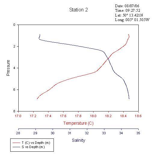
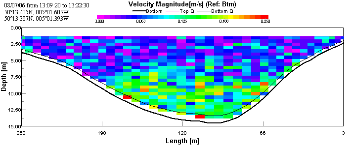
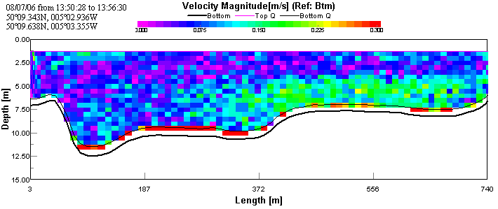
ADCP and CTD analysisThe first transect taken at the upper reaches of the estuary shows the faster moving (~0.125 m/s) layer of water on the bottom. This is assumed to be sea water penetrating north up the estuary, as sea water is colder and more saline than river water; therefore forming a denser lower layer. This is overlain by a slower moving (~0.05 m/s) layer, assumed to be river water. The CTD data show a large change in salinity with depth indicating that there are indeed two bodies of water overlaying each other. See figures 2 & 3.
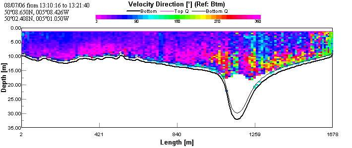
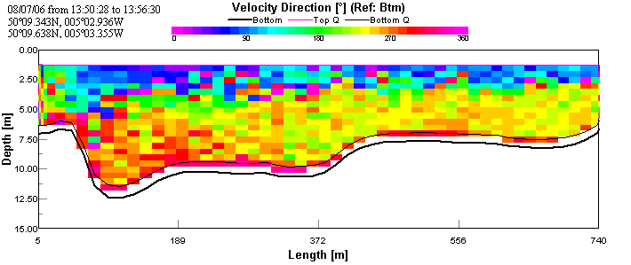
The transect taken across the mouth of the estuary shows very little
or no movement of water over the channel and eastern side of the
estuary. The backscatter contour plot shows very high surface
backscatter (surface roughness) and decreasing backscatter with depth.
This indicates that the seawater was underlying the river water; river
water results in higher backscatter as it contains higher sediment and
particulate load. On the east side there is faster (~0.5 m/s),
north-easterly moving, water that may be a result of mixing between
southerly-flowing surface river water and northerly-flooding seawater.
The underlying layer of presumed seawater has a more northerly direction
as it undercuts the river water. The transect was taken near the end of
flood tide resulting in the low maximum velocity at the mouth of the
estuary. See figures 4 & 5.
Again, the transect across Falmouth harbour shows faster, westerly-moving bottom water presumed to be the penetrating seawater with an overlying layer of slower, north-easterly moving water. This is presumed to be the river water flowing into the estuary. The CTD data confirms that the top layer is warmer and less saline and that the bottom layer is colder and more saline. See figures 6, 7 & 8.
Oxygen Concentration AnalysisOn collection of water samples on the boat, the concentration of dissolved oxygen was fixed using 1ml each of Manganese Chloride and Alkaline Iodide. The glass bottles were stored under water to maintain air tight conditions until the time of lab analysis.
The data collected for oxygen saturation showed no significant patterns. This indicates that an increased number of samples may be required to build up a more continuous profile of the oxygen saturation. However, this would have been more time consuming and a YSI probe could be used to give an unbroken profile of oxygen saturation. Nitrate AnalysisThe concentration of nitrate in the water samples was analysed using a spectrophotometer and a flow injection system. A peristaltic pump feeds the flow of 1% sulphanilimide, 0.1% Naphthyl ethylene-diamine dihydrochloride and a carrier solution. The water samples were injected into the system. The reagents caused a reduction from nitrate to nitrite on passing through a
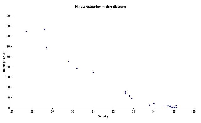
The points plotted on the nitrate estuarine mixing diagram are close to the theoretical dilution line. Therefore, nitrate appears to be behaving conservatively. This is the opposite of what we expected to see given the time of year; the chlorophyll data collected at the same time indicates that there are high levels of primary production occurring. It is possible that the input of nitrate is being matched by the biological removal due to low summer riverine input. Therefore, non conservative behaviour is most likely, with the apparent conservative behaviour being caused by a balance between input and removal. This notion is supported by the situation of some points slightly below the theoretical dilution line. Phosphate AnalysisTo calculate phosphate concentration, the following steps were made: prepare working standard solution; stock solution was diluted using MQ water:
prepare calibration and 3 blank solutions
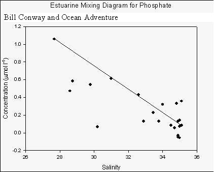
The estuarine mixing diagram shows that phosphate behaves non-conservatively within the Fal estuary.
It appears to be removed throughout the majority of the estuary.
However, the water sample collected at the site nearby the fish farm
was found to be higher in phosphate than the rest of the estuary.
This is to be expected as excess nutrients are added to the water in order to enhance growth of the shellfish being farmed. Silicon analysis
Locations involved for RIBs
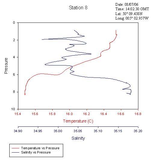
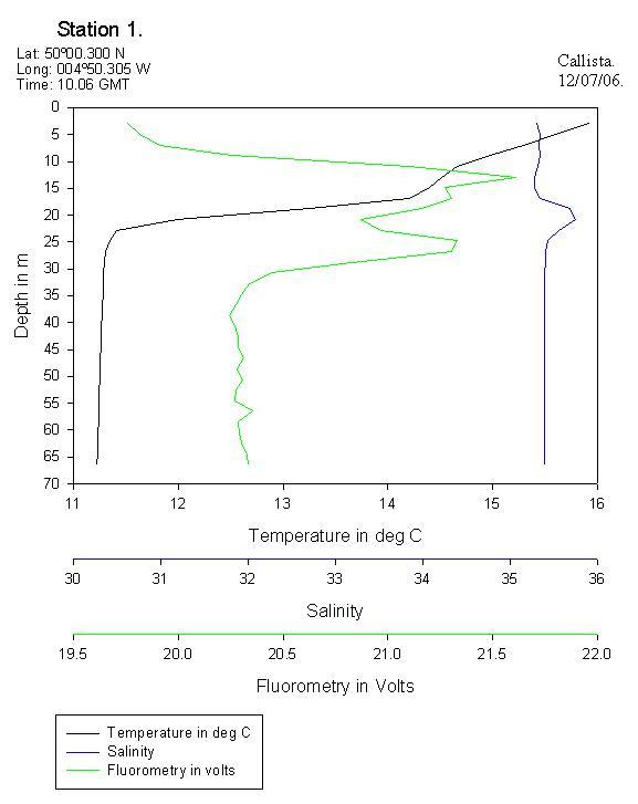
Vertical Profile of the Physical Characteristic of the Fal EstuaryThe vertical profile of temperature and salinity shown in figure 14 represents the physical structure of the estuarine water column. The temperature decreases slightly with depth. This is because river water (which is warmer than sea water at this time of year) is flowing over the surface. Solar irradiance also causes surface water to be warmer than deeper water. Salinity is seen to increase with depth, as the sea water is flowing into the estuary along the bed. The water column is therefore observed to be statically stable. The ADCP data collected during the estuarine survey supports the notion of a typical two layer estuarine 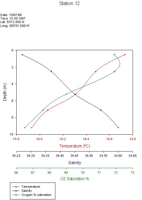 circulation with a landward flow at depth and a seaward flow at the surface. However, the low summer riverine discharge means that the estuary is tidally dominated in terms of flow. Therefore, the tide is penetrating further up the estuary than perhaps it normally would. This evidence suggests that perhaps the Fal estuary is partially mixed. The temperature and salinity changes are very small, which indicates a well mixed estuary. Conversely, a secondary circulation can not be supported by a well mixed estuary and hence the suggestion of a partially mixed estuary. More study is required at different times of year and states of tide in order to gain a fuller impression of the Fal estuary’s physical characteristics. The dissolved oxygen plot also shown in figure 14 shows a subsurface maximum and a gradual decrease with depth. This is likely to be due to a subsurface photosynthesis maximum, which often occurs as a result of photoinhibition at the surface and light limitation at depth.
|
|||||||||||||||||||||||||||||||||||||||||||||||||||||||||||||||||||||||||||||||||||||||||||||||||||||||||||||||
Offshore Chemical and Biological Analysis
The offshore survey carried out on R/V Callista on the 8th of July 2006 aimed to investigate the vertical structure of the water column in terms of physical, chemical and biological parameters. The survey was carried out as a time series of observations whilst at anchor approximately 10miles south-east of Falmouth estuary. ADCP data and CTD data was used to draw conclusions about the structure of the water column and to determine sampling depths along the vertical CTD profiles. A vertical plankton net was also used to sample the zooplankton and analysis of the plankton and chemistry was carried out in the lab the next day. Callista Biology Data AnalysisSamples were taken at hourly intervals from 10:30 GMT as part of a
time series profile at approximately Lat 50°00.063 & Long 004°50.262. For phytoplankton, samples were taken at two intermediate depths depending on the position of the thermocline. Samples were then stored in lughols iodide and labelled. In the lab samples were decanted to 100ml and from this 10ml taken; a further 1ml was then viewed under the microscope to allow identification of the different phytoplankton species. In total twelve samples were taken from three cast but we were unable to do anymore as the cable was damaged on the third cast. These gave deeper depths of 24.1, 22.0 & 17.9m and shallower depths of 13.0, 11.0 & 17.3m.
Callista Chlorophyll AnalysisChlorophyll is a good indicator of phytoplankton biomass. Chlorophyll maxima are present for all samples on the time series.
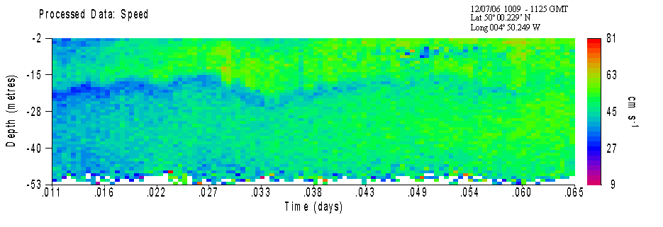
Callista ADCP and CTD AnalysisADCP velocity data collected over the sampled time series clearly shows a layer of water with decreased speed (~ 25m/s slower) at approximately 22m depth (ADCP1); corresponding with the base depth of the thermocline. Although no physical explanation for this reduced velocity has been proven, it may be that the very steep thermocline in this area causes acoustic refraction of the ADCP pulse. Therefore this layer may not in fact be a real phenomenon but an artefact of the ADCP itself.
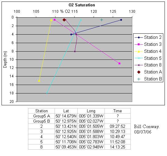
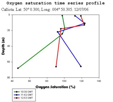
Callista Oxygen AnalysisThe oxygen content at surface can be seen to increase throughout the
day with a value of 97.6% at 10:30 GMT rising to a value of 118.9% at
12:53 GMT. This may be due to the increased activity at the sea surface, leading to greater oxygen diffusion
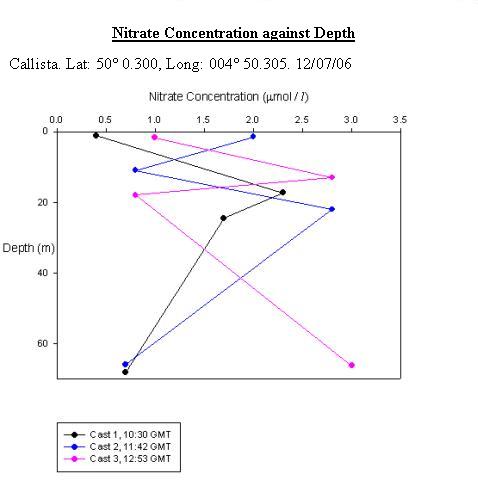
Callista Nitrate AnalysisCast 1 had a surface concentration 0.4 µmol/L, this then increased to a peak of 2.3µmol/L by 17.3m, which was just above the thermocline. There was then a decrease in concentration by 0.6 µmol/L below the thermocline at 24.5m and it then fell further to 0.7µmol/L by 68m. Cast 2 had a higher surface concentration than Cast 1, which was 2.0µmol/L. This then fell to 0.8 µmol/L by 11m, however, the concentration then peaked at 2.3 µmol/L by 22.0m. From here the concentration then fell to 0.7 µmol/L by 65.8m. At the surface, Cast 3 was similar to Cast 1 because it had a concentration of 1.0 µmol/L and rose to 2.8 µmol/L by 13m. The concentration then fell to 0.8 µmol/L by 17.9m but unlike Cast 1 the concentration then increased to 3.0 µmol/L by 66.2m. It is difficult to interpret this data because each cast had different behaviour. However, it could be viewed as the daily change in the tidal cycle.
See figure 20.
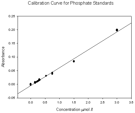
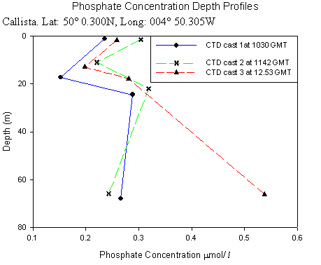
Callista Phosphate AnalysisThis time series depth profile shows high surface phosphate concentrations, with a marked decrease in concentrations between 11m and 17 m for all three CTD casts. This is as expected and is likely to be a result of high phytoplankton densities in this depth range which is indicated as a chlorophyll maximum by the chlorophyll data. This is then followed by an increase in phosphate concentrations at about 20m corresponding with a rapid decrease in chlorophyll. In rofiles 1 and 2 the concentrations gradually decrease with depth (0.0011mmol/l/m2 ) down to the maximum depths. However, in profile 3 there was a large increase with depth in phosphate concentration (0.0053 mmol/l/m2 ). This also relates to the chlorophyll time series profile, in that profile 3 at 12:53 GMT decreases much more rapidly with depth, so that phosphate concentration increases. As shown in figure 22, with the calibration curve (figure 21) in the figures below:
Callista Silicon Analysis
|
|||||||||||||||||||||||||||||||||||||||||||||||||||||||||||||||||||||||||||||||||||||||||||||||||||||||||||||||
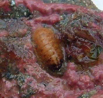
General ConclusionsGeophysics ConclusionsResults of side scan sonar identified 4 sediment types; Bedrock of slate, bedrock with sediment cover, rippled sediment and homogeneous sediment. 4 Grabs were taken in suspected areas of interest after initial side scan analysis. Live maerl beds were located in previously unknown areas of the estuary. Various other organisms of interest were also identified. Further more, grabs confirmed side scan sonar analysis.Estuarine and RIBsThe estuarine study indicated that diatoms were the dominant phytoplankton group throughout the estuary. Zooplankton populations, however, displayed a transition from largely copepod dominated at the head to co-dominance between copepod and hydromedusae at the mouth of the estuary. Chlorophyll concentrations appeared to be consistent with depth although there was a lateral decrease approaching the mouth of the estuary. Oxygen concentrations displayed no significant trends.
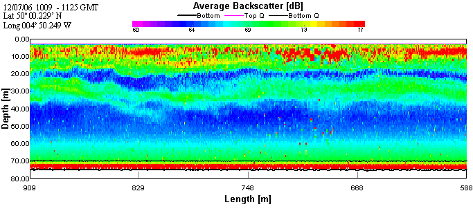
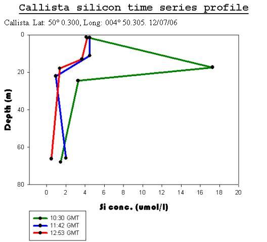
Offshore ConclusionsResults from the biology analysis found that the phytoplankton community is dominated by Karenia mikimotoi and that the zooplankton community is dominated by Copepoda. Chlorophyll maxima were found between 11 and 17m deep and the highest concentration was 6.6µg/l. Oxygen concentrations at the surface increased throughout the day from 97.6% to 118% saturation. The highest value overall was at the chlorophyll maxima which was 123%. Below the chlorophyll maxima, the oxygen concentration decreased with depth. No clear conclusions could be drawn from the Nitrate data because each cast had different behaviour. However, it could be viewed as the daily change in the tidal cycle. Low phosphate concentrations were found in the region of the chlorophyll maxima. This is a result of biological uptake by photosynthetic organisms. All Silicon levels decreased below the chlorophyll maximum. Cast one appears to show an anomaly as there was a drastic increase by approximately 13µmol/l at the chlorophyll maxima. The other casts showed no significant change in Silicon concentration above the chlorophyll maximum. Backscatter data from the ADCP and chlorophyll data from the CTD show corresponding peaks in phytoplankton and zooplankton. This indicates two communities; one near the surface and one at the thermocline. |
|||||||||||||||||||||||||||||||||||||||||||||||||||||||||||||||||||||||||||||||||||||||||||||||||||||||||||||||
Image of Karenia mikimotoi taken from
www.ifremer.fr.htm![]()
Image of Thalassiosira rotula taken from
www.icbm.de.htm
Other useful links;
www.mba.ac.uk/NMBL/publications/charpub/occasionalpub8.htm
www.algaebase.org/SpeciesDetail.lasso?species_id=4
 A survey was undertaken in order to study sediment structures of a
portion of the Fal estuary between Pendennis Point and Black Rock. The
aims were to identify different sediment types and bedforms, outcrops of
bedrock, any manmade structures and any ecologically important species
such as maerl and eel grass. Sidescan sonar was used in conjunction with
grab samples as a method of ground truthing.
A survey was undertaken in order to study sediment structures of a
portion of the Fal estuary between Pendennis Point and Black Rock. The
aims were to identify different sediment types and bedforms, outcrops of
bedrock, any manmade structures and any ecologically important species
such as maerl and eel grass. Sidescan sonar was used in conjunction with
grab samples as a method of ground truthing. 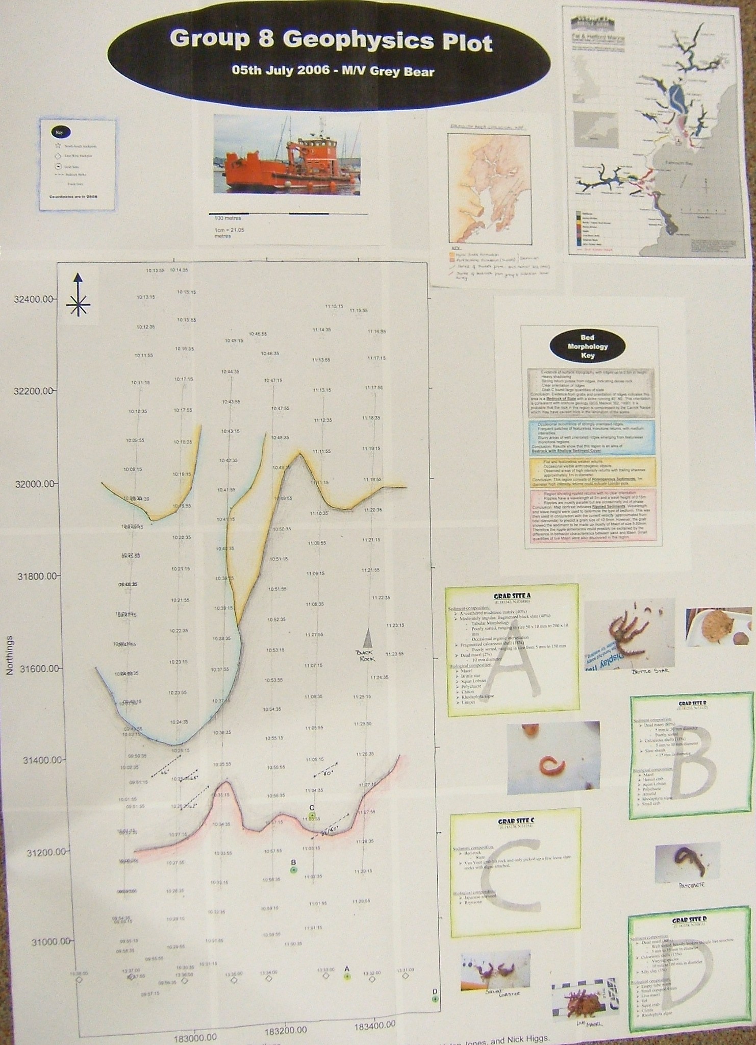
 40% Weathered mudstone matrix
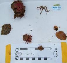
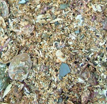 Sediment composition:
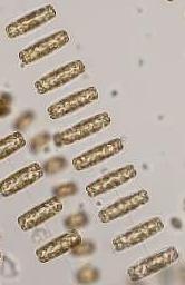 organisms
present within the estuary and there was little change in the there
distribution throughout the estuary. These were with the abundances
given the Diatoms Thalassiosira rotula (1875), Chaetoceros
spp. (1445) and the Dinoflagellate Karenia mikimotoi
(750). Downstream of the King Harry Ferry there were four species
present that were not found upstream, these were with the abundances
given the Ciliate Mesodinium rubrum (50), the Diatom
Rhilzosolenia alata (20), the Dinoflagellates Alexandrium spp.
(5) & Protoperidium spp (25) and a Silica-flagellate. The
species only found upstream of the King Harry Ferry were the Diatoms
Eucampia spp. (5) & a Centric Diatom (5), as well as the
Dinoflagellate Ceratium fusus (5). These were all in very
low concentrations which could explain their absence from the
upstream/downstream sample sites. The remaining species are as
follows with abundances given; the Diatoms Rhizosolenia
stolterfothii (200), Rhilzosolenia delicatula (280),
Rhizosolenia setigera (145), Nitzschia spp. (240) and
Melosira spp. (20), the Dinoflagellate Prorocentrun micans
(220) and an unidentified Ciliate (60).
organisms
present within the estuary and there was little change in the there
distribution throughout the estuary. These were with the abundances
given the Diatoms Thalassiosira rotula (1875), Chaetoceros
spp. (1445) and the Dinoflagellate Karenia mikimotoi
(750). Downstream of the King Harry Ferry there were four species
present that were not found upstream, these were with the abundances
given the Ciliate Mesodinium rubrum (50), the Diatom
Rhilzosolenia alata (20), the Dinoflagellates Alexandrium spp.
(5) & Protoperidium spp (25) and a Silica-flagellate. The
species only found upstream of the King Harry Ferry were the Diatoms
Eucampia spp. (5) & a Centric Diatom (5), as well as the
Dinoflagellate Ceratium fusus (5). These were all in very
low concentrations which could explain their absence from the
upstream/downstream sample sites. The remaining species are as
follows with abundances given; the Diatoms Rhizosolenia
stolterfothii (200), Rhilzosolenia delicatula (280),
Rhizosolenia setigera (145), Nitzschia spp. (240) and
Melosira spp. (20), the Dinoflagellate Prorocentrun micans
(220) and an unidentified Ciliate (60).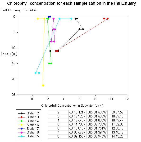

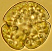 3 groups / orders were identified and Dinoflagellates were found to be more abundant than Diatoms or Ciliates. However, Diatoms showed a greater diversity (12 species) than Dinoflagellates (5 species) and Ciliates (1 species). The reason for this was because of the presence of the Dinoflagellate
Karenia mikimotoi (shown in the image to the left), which was the dominant species at both depths. In total there were 4015 organisms identified and of this 3275 were
K.mikimotoi. However, there were differences between the deeper and shallower sampling depths.
3 groups / orders were identified and Dinoflagellates were found to be more abundant than Diatoms or Ciliates. However, Diatoms showed a greater diversity (12 species) than Dinoflagellates (5 species) and Ciliates (1 species). The reason for this was because of the presence of the Dinoflagellate
Karenia mikimotoi (shown in the image to the left), which was the dominant species at both depths. In total there were 4015 organisms identified and of this 3275 were
K.mikimotoi. However, there were differences between the deeper and shallower sampling depths.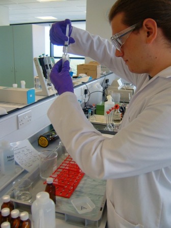 The deeper depth had a lower diversity (9) and a lower abundance (1095) than the shallower depth (diversity = 10 & abundance = 2920). In terms of group/order diversity, the deeper depth had 5 Diatoms, 3 Dinoflagellates and 1 Ciliate. The reason for this was again because of the presence
Karenia mikimotoi, which was the dominant species. At both depths it was in roughly the same proportion of 80% of the total population. Although most species were present at both depths, there was an increase in abundance for all species at the shallower depth. The shallower depth had 3 Diatoms (Guinardia flaccida, Heptocylindrus
spp & Rhilzosolenia delicatula) and 1 Dinoflagellate (Gyrodium spp.) that were only present at this depth. The deeper depth had 1 Diatom (Rhilzosolenia alata) and 2 Dinoflagellates (Prorocentrun micans &
Protoperidium spp), that were only present at that depth. Protoperidium spp
is also a rare species for this area. The following species were found
at both depths; Diatoms
Rhizosolenia setigera, Thalassiosira rotula, Rhizosolenia stolterfothi, an unidentified Centric Diatom, the Dinoflagellate
Karenia mikimotoi and an unidentified Ciliate.
The deeper depth had a lower diversity (9) and a lower abundance (1095) than the shallower depth (diversity = 10 & abundance = 2920). In terms of group/order diversity, the deeper depth had 5 Diatoms, 3 Dinoflagellates and 1 Ciliate. The reason for this was again because of the presence
Karenia mikimotoi, which was the dominant species. At both depths it was in roughly the same proportion of 80% of the total population. Although most species were present at both depths, there was an increase in abundance for all species at the shallower depth. The shallower depth had 3 Diatoms (Guinardia flaccida, Heptocylindrus
spp & Rhilzosolenia delicatula) and 1 Dinoflagellate (Gyrodium spp.) that were only present at this depth. The deeper depth had 1 Diatom (Rhilzosolenia alata) and 2 Dinoflagellates (Prorocentrun micans &
Protoperidium spp), that were only present at that depth. Protoperidium spp
is also a rare species for this area. The following species were found
at both depths; Diatoms
Rhizosolenia setigera, Thalassiosira rotula, Rhizosolenia stolterfothi, an unidentified Centric Diatom, the Dinoflagellate
Karenia mikimotoi and an unidentified Ciliate.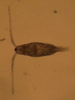 The bottle volume sampled
was 500 ml and from this the water sampled for each site is as follows;
P1 gave 1.37 m3, P2 gave 3.9 m3 and P3 gave 2.94 m3. Then 5ml was taken
as an aliquot size for microscope analysis. P1 had heavy layback induced
by a strong tidal flow that resulted in the volume of water sampled being greater than calculated. Hence there was a larger abundance of organisms for P1
(30145), compared with 5232 and 5850 for P2 and P3 respectively. In total there were 41227 organisms from 15 groups / orders identified, with 9 groups / orders being present on all samples. They were
(in order of abundance); Copepoda (19369) , Hydromedusae (Jellies) (7182), Chaetognatha (5293), Copepoda nauplii (2403), Decapoda larvae (Crabs/Shrimp) (1804), Appendicularia (Larvacea) (1052), Siphonophorae (989), Cladocera (582) & Polychaeta larvae (371).
The bottle volume sampled
was 500 ml and from this the water sampled for each site is as follows;
P1 gave 1.37 m3, P2 gave 3.9 m3 and P3 gave 2.94 m3. Then 5ml was taken
as an aliquot size for microscope analysis. P1 had heavy layback induced
by a strong tidal flow that resulted in the volume of water sampled being greater than calculated. Hence there was a larger abundance of organisms for P1
(30145), compared with 5232 and 5850 for P2 and P3 respectively. In total there were 41227 organisms from 15 groups / orders identified, with 9 groups / orders being present on all samples. They were
(in order of abundance); Copepoda (19369) , Hydromedusae (Jellies) (7182), Chaetognatha (5293), Copepoda nauplii (2403), Decapoda larvae (Crabs/Shrimp) (1804), Appendicularia (Larvacea) (1052), Siphonophorae (989), Cladocera (582) & Polychaeta larvae (371).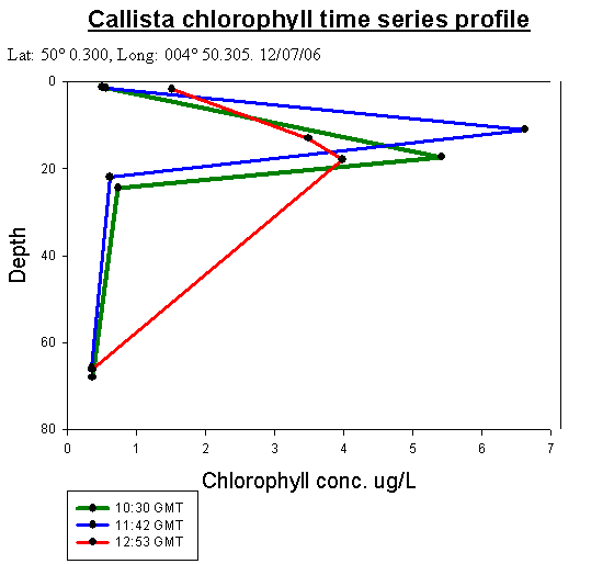