 |
|
|
|
|
|
Falmouth '06 |
 Group 7 (Back Left to Right: Tom Fisher, James Cobb, Andrew Barrett-Mold, James Rosling. Front Left to Right Sarah Burgess, Charlie Best, Maria Salta, Amy Pattington) |
| Contents |
|
|
| 1. Foreword | ||
|
Fig 1.1: map showing the Fal estuary system |
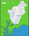
Abstract: Using RIBs, the Bill Conway, RV Callista, and the Grey Bear the Fal estuary Ria system was surveyed extensively. This survey took place from the 3rd to the 16th July 2006, when there had been little rain for a long period, what rain that there had been was mainly absorbed by the peat moors at the source of the river inputs. The weather for this period was mainly warm, leading to the fresher river water to be warmer than the tidal waters. The head of the estuary was found to be dominated by the toxic Nitzschia Longissima with 7630000 species per litre at station 7 sampled on the RIBs. Chemical mixing diagrams show that the main dilution of nutrients is by a first order process, with the exception of an increase in phosphate near Truro that can be associated with sewage and runoff from the town. The geophysical data shows that floor near the head of the estuary is mainly fine grained, anoxic mud, whereas further toward the mouth it is much more coarse and composed mainly of broken shells. There were no biological habitats noted on the floor of the estuary, indicating that the sediment is not suitable for this. High salinities were noted well up into the river, and no riverine end member was found using the boats. This concurs with the low concentrations of nutrients found. Using T/S probes and a CTD, depth profiles show that the surface layer of the water column was very stable with fresher, warmer river water flowing over colder, denser tidal water. Data from the ADCP shows the flow velocities of these two layers and how they influence each other. The RV Callista was used to collect data from offshore that showed that the coastal waters at this period were stratified, with the greatest concentrations of chlorophyll situated around the thermocline as should be expected. Nutrient concentrations were variable in these waters and not enough data was collected to draw firm conclusions from this due to bad weather. Introduction: Aims: 1) To determine the physical character of the offshore environment, using CTD and ADCP data, and compare this to data from within the estuary, relating it to the chemistry and biology 2) To observe how phyto- and zooplankton populations and taxonomy vary spatially, using samples from both the estuary and offshore environments 3) To observe and interpret how nutrient levels (nitrate, phosphate and silicate) vary spatially, using data from the estuary and offshore samples, and subsequently relate this to the occurrence of phyto- and zooplankton in the water column 4) To observe differences in oxygen saturation throughout the estuarine and offshore water columns, and relate this to phyto- and zooplankton distribution 5) To relate oxygen saturation and nutrient levels to the physical structure of the estuary and offshore region, by constructing vertical and horizontal profiles of temperature and salinity data Between 3rd-16th July 2006, the Fal estuary and an offshore region to the east of the mouth as indicated on figure 1.1 was surveyed. Observations of the biological, chemical and physical parameters of the estuary were taken from the RIBs (upper estuary) and Bill Conway (lower estuary); offshore readings taken from Callista; geophysics data was collected using Grey Bear, as well as benthic biological data. The River Fal is approximately 29km in length, with its source at Goss Moor near St Dennis (see figure 1.2 Map of Fal), this is a granite based moor with a mosaic of gorse, dry and wet heath, mires and willow scrub. The Fal Estuary is classified as a ria and is the third largest natural harbour in the world. Rias ‘were formed during the Flandarian transgression by the flooding of previously incised valleys’ (Dyer, 1997). Cornwall’s granite based geology causes significant metaliferous and clay deposits with mining of metals particularly tin, which can have adverse effects on the biota of the estuary. A major source of pollutants has been Restronguet Creek, after an industrial accident in 1992. |
Fig 1.2: showing source at Goss Moor and catchment area of estuarine system |
|
Introduction: Truro river, which is a part of the Fal estuary system, was surveyed twice by Group 7, on 5/7/2006 and 12/7/2006. Three Research Vessels were used: Two RIBs (Coastal Research and Ocean Adventurer) and R.V. Bill Conway. Both RIBs and Bill Conway collected water samples in order to study the chemical, physical and biological processes occurring within the Truro River.
|
||||||||||||
|
2a. RIBs
|
|
|||||||||||
|
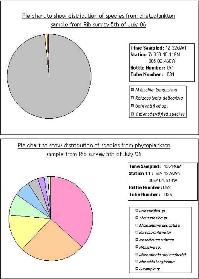
Figure 2.1: shows a comparison of phytoplankton data between stations 7 and 11 on RIBs
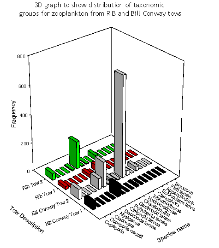
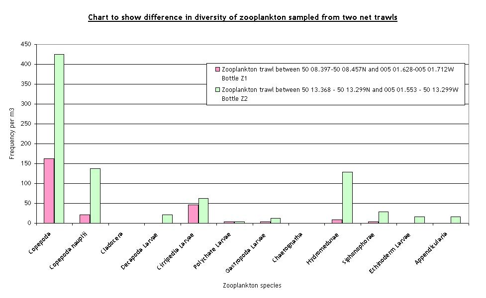
Figure 2.2: zooplankton from estuarine tows for both Bill Conway and RIBs
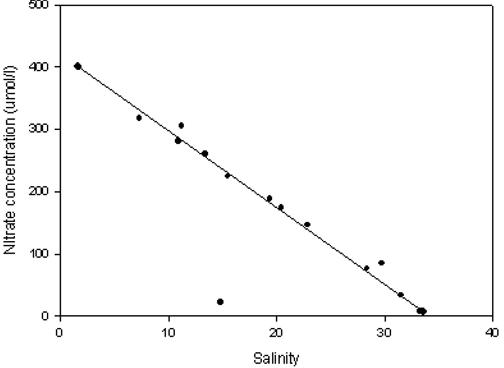
Figure 2.5: from upper Fal/Truro River showing conservative behaviour of nitrate
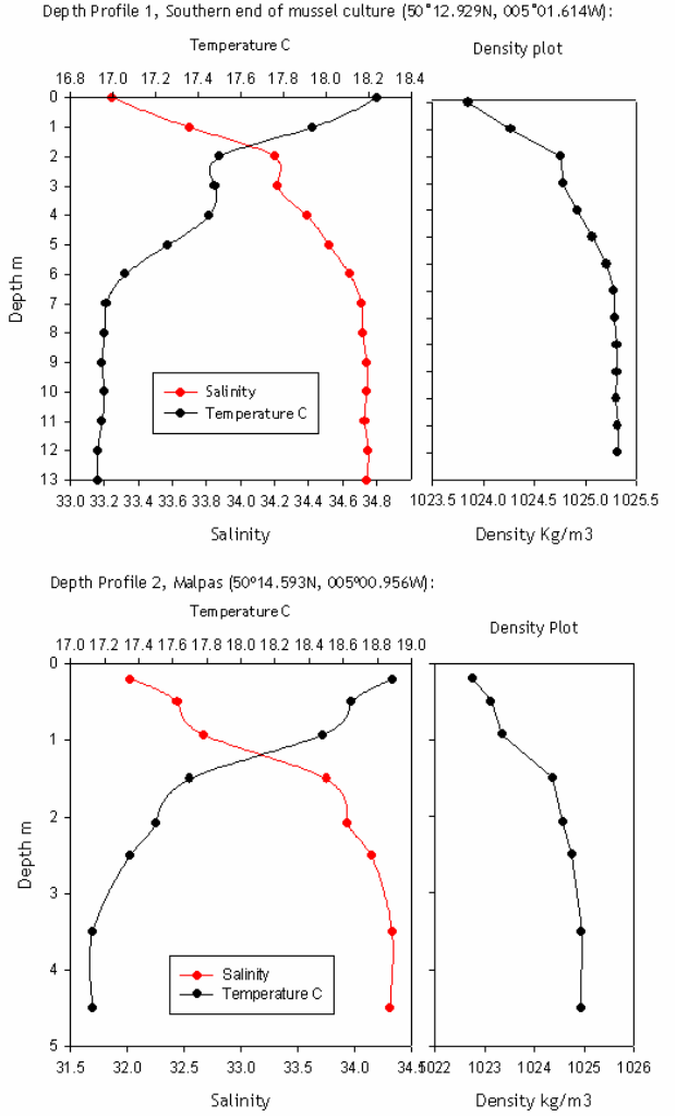
Figure 2.6: showing physical structure of water column at the southern end of the mussel culture and at Malpas |
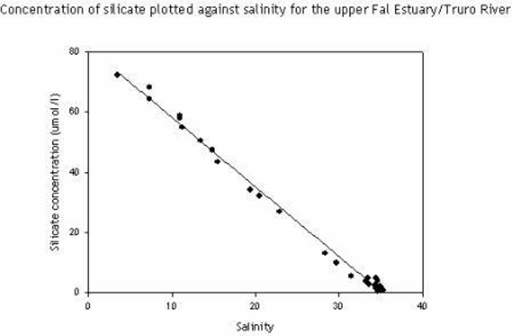
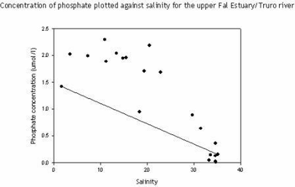
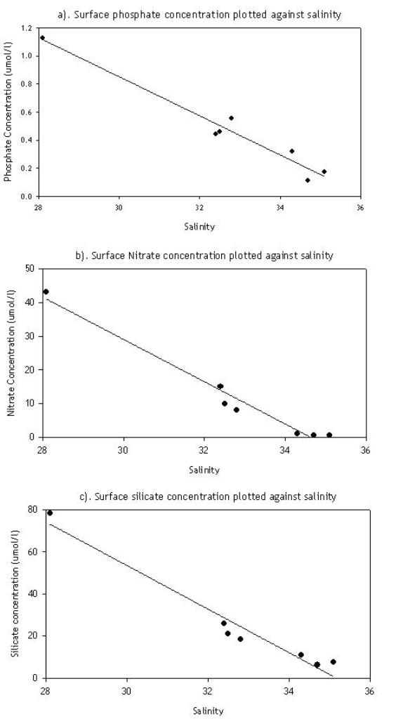
Date: 05/07/2006 Introduction: Truro River was surveyed continuously from Truro to the suspended rope mussel culture (final sampling point: 050o12.653N, 005o01.620W) sampling at approximately every 2 salinity increments. Salinity, temperature, pH, dissolved oxygen (% and mg/l), and euphotic depth (Secchi disk depth) were recorded. Water samples were taken at each station for nitrate, phosphate and silicate concentration, as well as chlorophyll and dissolved oxygen. These samples were then used to calculate specific concentrations for each parameter, using various laboratory techniques. In total, seventeen stations between Truro and the suspended rope mussel farm were sampled. Equipment used: · YSI probe · Niskin bottle · Secchi disk · Sampling bottles (plastic for silicate; glass for nitrate, phosphate & oxygen) · Syringes (including attached glass fibre filters) · GPS · 200µm mesh zooplankton net (diameter 60cm) Methods: Five phytoplankton samples were taken at particular sites, for dominant species identification. Two trawls to collect zooplankton were performed, again to identify dominant species present. Both samples were then processed in order to give an indication of the numbers of individuals present in a particular volume, e.g. phytoplankton per litre. Phytoplankton: At the five stations a 100ml water sample was collected and placed in a glass bottle containing Lugols iodine (used to kill, preserve and stain individual phytoplankton, for accurate results). These samples were analysed later using a binocular stereo microscope to determine phytoplankton numbers and taxonomic constituents. Zooplankton: Zooplankton samples were taken over two sites using a 200μm trawl net, and placed in plastic bottles with 10% Formalin solution (used to kill and preserve the zooplankton). These were also viewed later using a low power binocular microscope for zooplankton identification and counting. Results and Discussion: A Phytoplankton comparison was carried out between stations 7 and 11. (see Fig. 2.1) Using the Secchi disk, the euphotic depth was calculated to be 7.02m at station 11 and 3.18m at station 7. The near surface euphotic zone depth (3.18m) at station 7 corresponds to a high number of phytoplankton in the water column, blocking out sunlight and making the euphotic zone shallower. There was an increased amount of suspended matter within the water column at this station, increasing light attenuation. This is possibly caused by the surrounding environment adjacent to the channel, which was dominated by extensive mud flats. At station 11 the euphotic zone depth was much deeper, at a depth of 7.01m, with a smaller phytoplankton population. At this station, there was a reduced level of suspended matter in the water compared to station 7. Again possibly due to the surrounding environment which had a predominantly rocky shoreline. Station 7 was dominated by Nitzschia longissima, at a total calculated concentration of approximately 7,630,000 per l. This makes up around 98.3% of the phytoplankton population sampled from this station. The other 2% were made up of mostly Rhizosolenia delicatula, other species including Rhizosolenia setigera, Leptocylindricus sp, Mesodinium rubrum and other unidentified species. Nitzschia longissima is a toxic species, found only under certain water conditions. At station 11, there was only a small Nitzschia longissima population, ~4% of the sample, with a total of ~38% of the species present being unidentified. The next most abundant species were various Thalassiosira species forming 25% of the total population, with Rhizosolenia delicatula being the third most abundant species found. The average of the two chlorophyll concentrations for station 7 was 13.2μg/l, whereas for station 11 it was 12.1ug/l. There is a general trend of increasing chlorophyll concentration with salinity, (2.18µg/l at salinity 1.69 and 13.2µg/l at salinity 22.88). There is some evidence to suggest that the chlorophyll concentrations drop off at high salinities (9.7μg/l at salinity 33.55). Total number of phytoplankton observed at station 11 was 201800, compared with a total number of 7765000, almost 30 times the population value of station 11 (fig 2.1). Conclusion: The near surface euphotic zone depth (3.18m) at station 7 corresponds to having a high number of phytoplankton in the water, blocking out light and making the euphotic zone shallower. There was also a lot of suspended matter in the water at this area, with the surrounding estuary banks being mud flats. At station 11 the euphotic zone depth was much deeper, at a depth of 7.01m, with much lower numbers of phytoplankton blocking irradiance from the surface. At this station, there was low suspended matter in the water, with the banks being predominantly rock. Methods: Nutrients: At each station surface samples were collected, these were filtered through glass fibre filter paper. 50mls of the filtered sample were collected in a glass bottle for phosphate and nitrate analysis later, a further 35mls were collected in plastic bottles for silicate analysis. Chlorophyll: In total two filter papers were used at each station, and each paper was used to filter 50mls of the sample. They were collected in tubes containing 7mls of acetone and stored in a cool bag with ice. Oxygen:The Niskin bottles were used to collect surface water and this was siphoned into two glass bottles and stored, without trapping any air bubbles inside, underwater to minimize any possible transfer of oxygen. Results and Discussion: The silicate concentration was highest in the lower salinities (72.3 umol/l at salinity 3.5) and lowest in the higher salinities (0.690 at salinity 35.1), this can be seen in the graph to the right (Fig. 2.3). The Silicate concentrations follow a first order theoretical dilution line when plotted against salinity. The phosphate concentration (Fig. 2.4) tended towards being higher in lower salinities like silicate concentration however phosphate behaves in a non-conservative manner with significant addition seen at the mid salinities. This could be associated with anthropogenic inputs from sewage and runoff from urbanised areas. The nitrate concentration also follows a first order theoretical dilution, with highest concentrations in the lower salinities, with the exception of the nitrate sampled from station 5, (050° 15.359, 005° 02.629), shown by the diagram to the left (Fig. 2.5). The pattern shown by the silicate and nitrate mixing diagrams is consistent with nutrients being inputted into the estuary system by a freshwater input, and being mixed purely by the mixing of freshwater and saline water. Conclusion: The plot of silicate against salinity follows the Theoretical Dilution Line (TDL, from the riverine end member to the saline end member) closely, showing that this is a first order process and that the only factor is the mixing of the fresh water with the saline. For phosphate there is a marked increase above the TDL showing that there is another source of phosphate present that is adding to fresh water concentrations. This is most likely to be caused by sewage from Truro or runoff from the town or roads. Nitrate also follows the TDL, showing a first order process, with no notable addition or removal of nitrate from this system. The dissolved oxygen concentration increased significantly (from 98.0 to 121.8) between salinities 10.96 and 19.41. This is caused by an increase in productivity between the two stations as there was in increase in chlorophyll concentration further down. Methods: T/S Probe: At each station a T/S probe was used to measure the Temperature (°C), Salinity, Dissolved Oxygen (%), and pH at the surface. The T/S probe was also used for two depth profiles. Results and Discussion: The depth profiles (figure 2.6) clearly show a surface layer of less dense water; at the southern end of the mussel culture this is around 1m deep and at Malpas it is around 2m deep. The fresh water entering the estuary is not only less saline than the sea water but also warmer, this means that the water column will be very stable. As the fresh water moves down the length of the estuary it is more subjected to mixing and a greater amount of the surface layer is lost to entrainment, this is why the thermocline is shallower on the first profile (which is further downstream). Summary: The upper Fal Estuary exhibits a very stable water column with a surface layer of warm, less saline water. The higher salinities show a fairly well mixed diversity of phytoplankton species, whereas the lower salinities are dominated by the toxic Nitzschia Longissima. The phytoplankton counts for the regions which are dominated by Nitzschia Longissima show a much higher number of individuals per litre of seawater even though the chlorophyll concentrations are lower. There is an input of phosphate near the top end of the estuary which may be encouraging this growth of phytoplankton. |
 |
Figure 2.3: silicate data from upper Fal/ Truro River with silicate reducing with increasing salinity-conservative behaviour.
Figure 2.4: phosphate data from upper Fal/ Truro River showing non-conservative behaviour of phosphate |
|||||||||
|
2b.
Bill Conway
|
|
|||||||||||
|
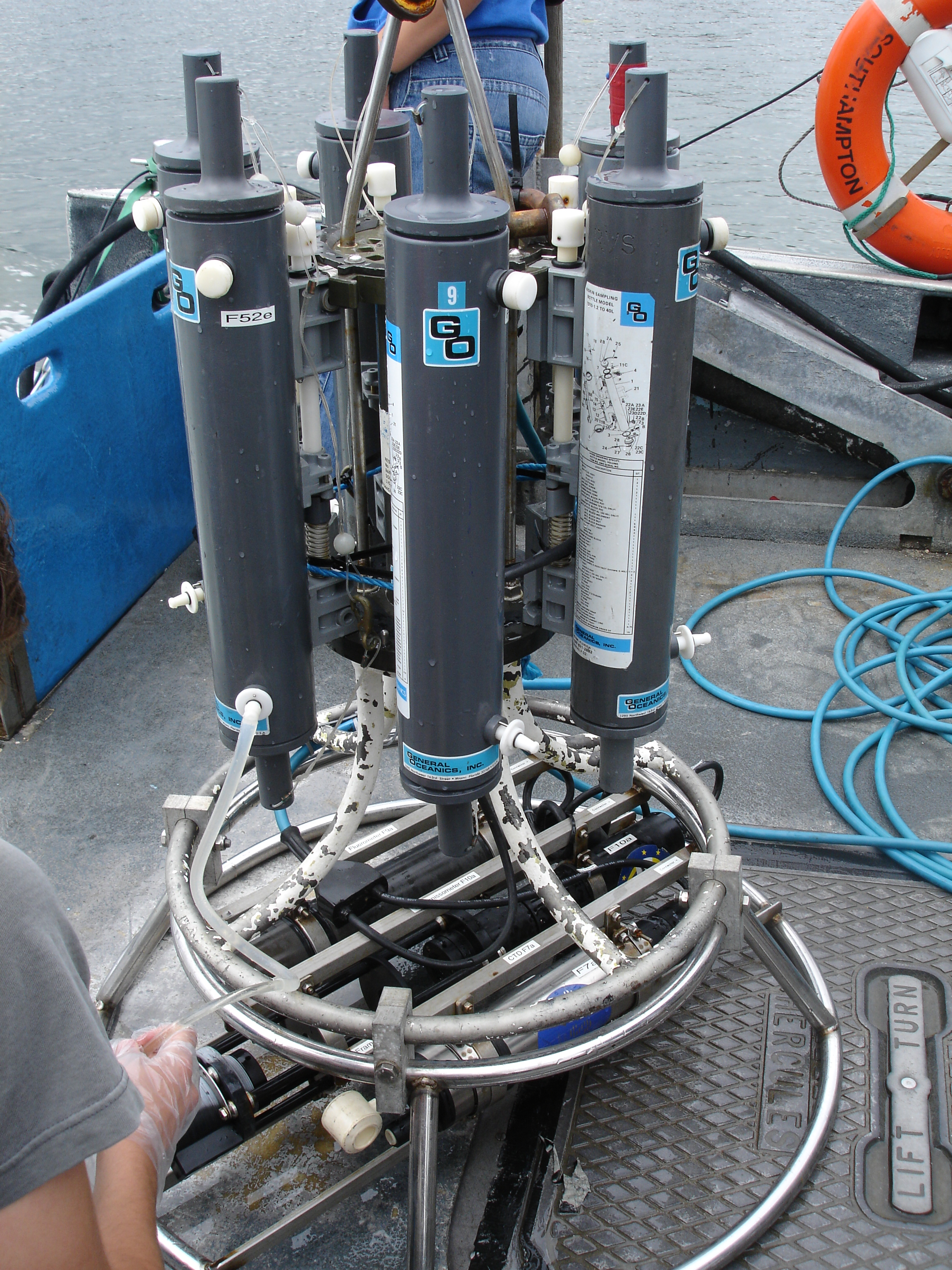
Figure 2.8: Six Niskin bottle rosette rig
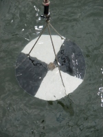
Figure 2.23: showing a secchi disk which can be used to calculate euphotic depth
Figure 2.21: comparison of zooplankton taxonomy from samples Z1 and Z2 (figure 2.20)
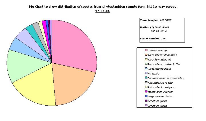
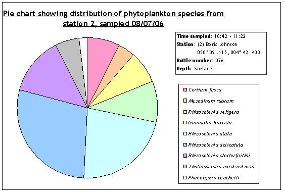
Figure 2.25: phytoplankton diversity taken from station 2
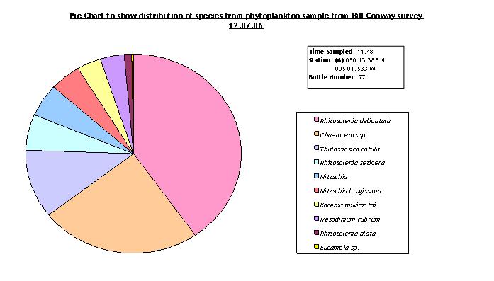
Figure 2.26 phytoplankton taken from station 6
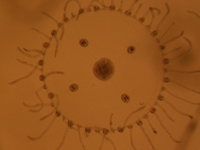
Figure 2.24: showing a hydromedusa under 7.5 times magnification
Figure 2.9: showing conservative behaviour of a) phosphate, b) nitrate and c) silicate
Figure 2.11: ADCP data for the horizontal transect at station 2
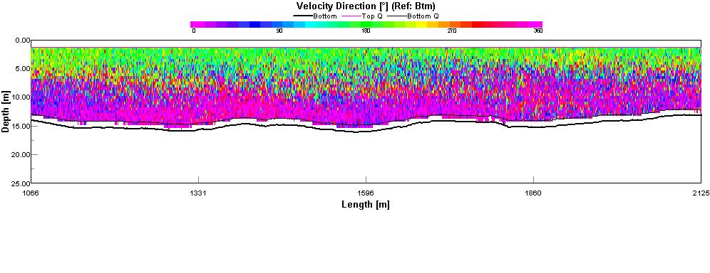
Figure 2.12: ADCP data for the vertical transect at station
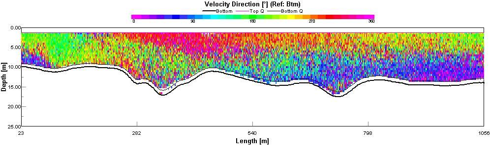
Figures 2.13: vertical profiles from the Fal river transect
|
Date: 12/07/2006 Introduction: On Wednesday 12th July 2006, extensive multi-parameter sampling was carried out from aboard RV Bill Conway. The area sampled extended from the upper reaches of the estuary 050°13.586N, 005°00.872W, to the mouth 050°08.608N (figure 2.7), 005°02.438W and 050°08.441N, 005°01.069W (forming the west and east sides of the mouth respectively). Similarly to the sampling carried out from the RIB’s, samples were taken for nutrient concentrations (nitrate, phosphate and silicate), dissolved oxygen and chlorophyll, with both phyto- and zooplankton also being collected for analysis. In addition, ADCP data was also collected to gain an idea of some of the physical structuring occurring throughout the Carrick Roads region of the Fal Estuary. A total of eight transects were performed throughout the sample area, with a CTD drop being carried out at a point of deep-water on six of them. A total of three samples were also taken from the surface, in areas where it was either unsuitable or too risky to deploy the CTD rig. Weather generally throughout the day was grey and overcast, with cloud cover of 8 octants. It was warm, with low winds and a sea state that was “flat as a witch’s tit” (thanks Bob!) However, weather conditions were recorded throughout the day at all stations, with additional information, such as land-use on the land adjacent to the estuary channel, also being noted. Equipment deployed: · Acoustic Doppler Current Profiler (ADCP) · Six Niskin bottle rosette rig (figure 2.8) · Secchi disk (figure 2.23) · Sampling bottles (plastic for silicate; glass for nitrate, phosphate & oxygen) · Syringes (including attached glass fibre filters) · GPS · 200µm mesh zooplankton net (diameter 60cm) with attached flowmeter · CTD rig with additional instruments (flourometer and transmissometer) Methods: Phytoplankton: At three of the stations (2, 4, and 6) 100mls of water were collected in a glass bottle containing Lugols iodine to preserve and stain any phytoplankton present; these were then viewed later under a microscope for phytoplankton counts. Zooplankton: A zooplankton net trawl was deployed twice at stations 2 and 6, see (figure 2.20) for 2 minutes at 1.5 knots each time. 10% formalin was then added to preserve the samples so that they could be viewed for zooplankton counts. Results and Discussion: The sample obtained from the zooplankton trawl (figure 2.21) at the head of the estuary (sample bottle Z2) contained a larger total biomass (phytoplankton plus zooplankton) than the other zooplankton trawl sample obtained at the mouth of the estuary (sample bottle Z1). This could be due to the increased input of nutrients from the surrounding catchment area which was predominantly farm land, introducing nitrate, phosphate and silicate from fertilizers used on the fields. Depth of the euphotic zone (calculated using secchi depth- three times secchi depth) was much shallower up the river, with a depth of 4.56m, meaning that the photosynthetically active region of the water is 4.56m and utilization of light by phytoplankton can only occur within this depth. This ties in with very high phytoplankton and zooplankton numbers, as they are found in the surface waters and effectively block out light from the surface. There was also a lot more sediment in the water column in general, possibly from the surrounding land. The average surface chlorophyll concentration for station 2 was 2.45μg/l whereas for station 6 it was 12.138μg/l. The much higher levels of chlorophyll are probably caused by the greater quantities of phytoplankton (700 million per m3 for station 2 and 5.13 billion per m3 for station 6, see figure 2.26). In some areas there were higher zooplankton numbers but lower phytoplankton numbers, indicating that the phytoplankton had been grazed by the zooplankton. The most abundant zooplankton taxa found at both trawl sites was copepoda (figure 2.22), with a marked increase in population size at the mouth of the estuary, 425 individuals in a m3 of water compared with 163 per m3 of water at the at station 6. Two phytoplankton dominant species found in the three samples were Chaetoceros sp., and Rhizosolenia delicatula. The average surface chlorophyll concentration for station 2 was 2.45μg/l whereas for station 6 it was 12.138μg/l. The much higher levels of chlorophyll are caused by the greater quantities of phytoplankton (700 million per m3 for station 2 and 5.13 billion per m3 for station 6). Methods: Nutrients: Each time the CTD was lowered Niskin bottles were closed at the deepest point, a midway point (either the chlorophyll maximum, or density gradient) and at the surface. Samples were drawn out from these and filtered with glass fibre filter papers before being stored in glass bottles (for phosphate and nitrate analysis) and plastic bottles (for silicate analysis). Chlorophyll: For each depth sampled with the Niskin bottles two filter papers were used, each one filtering 50mls of water. The papers were then stored in 7mls of acetone and kept cold. After being stored overnight the chlorophyll on the surface of the paper would leach out into the acetone, and the concentration was determined in the lab. Dissolved Oxygen: Oxygen sample bottles were used to collect water from each station at various depths. These were stored underwater to prevent any change in the amount of oxygen present, and were also analysed later for oxygen saturation. Results and Discussion: For each nutrient (Phosphate, Nitrate, and Silicate) the concentration decreases first order with salinity (figure 2.9), as the fresher riverine water mixes with the more saline sea water. With the exception of one sample at salinity 28.1, all of the nutrients were present at relatively low concentrations, for example at stations 2 and 3 (salinities 35.1 and 34.7 respectively) nitrate was present at 0.65μmol/l. The single sample taken at salinity 28.1 was also the sample that demonstrated the highest nutrient concentrations (1.127, 43.08, and 78.28μmol/l of phosphate, nitrate, and silicate respectively), this was collected from a single surface sample at 50°13.586N, 005°00.872W at the point where the river Fal joins the estuary, suggesting the Fal is adding nutrients. Methods: ADCP: The ADCP was used to determine the flow of water throughout the water column on each of the transects. This data can be used to calculate the speed, direction and magnitude of flow at a specific point, as well as total discharge of water across each transect. By viewing the backscatter properties of the data, estimations of zooplankton, turbulence, or density gradients can be made. CTD: The CTD rig was used to record conductivity (a measure of salinity), temperature, flourimetry (indication of pigment in the water), and transmission (the absorbance of light), with depth (calculated from pressure). Results and Discussion: ADCP:
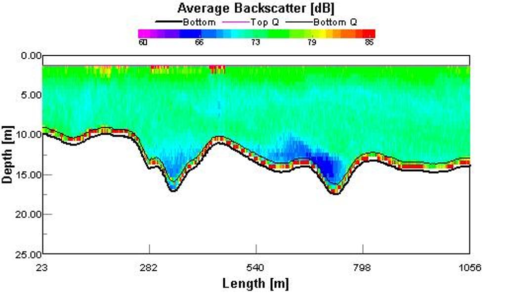
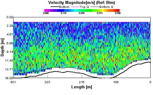
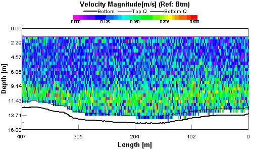
Horizontal transect across the mouth of the estuary (figure 2.11) at station 2 (figure 2.7). In the data taken from 1st transect (at the mouth of the river, figure 2.11) there is a strong tidal outflow at surface. The reason why the strongest flow is not in deep water channel is because this ADCP profile has been taken in the last few hours of an ebbing tide and so the majority of water higher in the estuary has been flowing out for several hours. The resolution of the ADCP doesn’t allow penetration to the deepest parts of the channel where, during the ebb, much of the water flow takes place. It is this flow that scours the channel, one of the main processes that maintain the deep water in the deep water in the port of Falmouth. The direction of water flow seen here is likely to be flowing round from the port and the Penryn River. The shape of the port and dock walls could act as barrier, holding back water during the major ebb part of the tidal cycle and effectively delaying its arrival at the estuary mouth. This explains the high velocity magnitude. The tidal outflow then effectively ‘misses’ the channel due to the gradient forcing the water to flow out of the estuary. Further evidence of this is seen at Station 3 further up the estuary, but due to the last 1/12 of the tide (from the rule of twelfths) the effect is not as great as the lower transect Station 2. The velocity direction plot (figure 2.12) shows all water heading out of estuary, some at different speeds, i.e. surface layer compared to bottom layer. As this layer is clearly defined, it is also possible to see the turbulence between the two. Some interference from resedimentation by strong tidal flows over silt/sand sea bed also occurred. Two clear layers showing the outflow of less dense fresh surface water over the top of denser more saline sea water. Red specks in between layers are eddies and small turbulences due to the interaction between the two layers. Velocity profile (figure 2.13) gives an indication of water movements at low tide; it is possible to see the two movements of water, with the salty denser water static at the bottom, and the fresh water layer moving over the top. The velocity direction profile (figure 2.13)varies with transect length as the boat path curved following the channel downriver. The dominant bend round past the narrows occurs at 400m down the transect, it is possible to see the rotation of the principle direction of the water as it moves round this bend. Figure 2.14 is from a transect run up the centre of the river and it shows a large presence of phytoplankton in the water column, whilst the estuary bed undulates the chlorophyll maxima is consistent between 5 and 8m depth. The surface high backscatter patches are from passing craft, namely the Enterprise passenger ferry, and some cock in a RIB that was going too fast. Transect taken after low tide (springs) into the incoming tide, velocity magnitude shows incoming denser more saline water during first 1/12 of the tidal cycle. Therefore when compared with CTD data for the station (figure 2.15) it is possible to see a step salinity gradient between the two bodies of water. Two and a half hours later and further down the estuary (figure 2.16), the salt water layer flooding in is thicker, with a bigger volume and in general a greater velocity.
|
Figure 2.10: glass sampling bottle containing dissolved oxygen sample
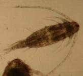
Figure 2.22: showing a copepod under 7.5 times magnification- this is the dominant taxa from Z1 and Z2
Figure 2.14: ADCP backscatter (dB) from transect up river Fal
Figure 2.16: ADCP vertical magnitude (m/s) from transect up the river Fal, closer to than the mouth compared to figure 2.15
Figure 2.15: ADCP vertical magnitude (m/s) from transect up river Fal |
|
3. Offshore
|
||||||||||||||||||||||||||||||||||
|
Figure 3.4: phytoplankton diversity at station 2 taken from a horizontal trawl at the surface
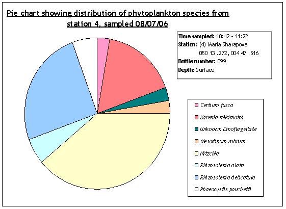
Figure 3.5: phytoplankton diversity at station 4 taken from a horizontal trawl at the surface
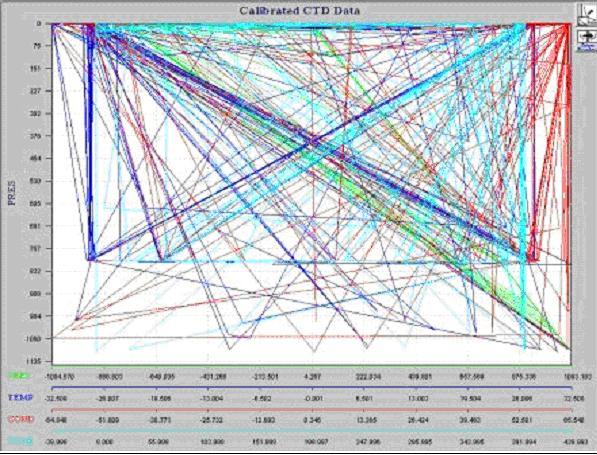
Figure 3.7: CTD data unusable due to faulty cable
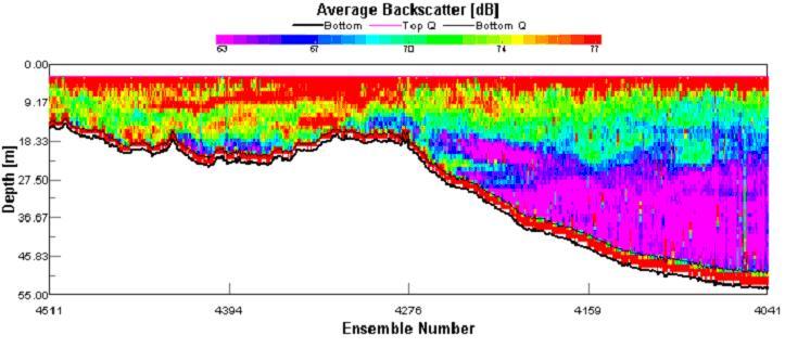
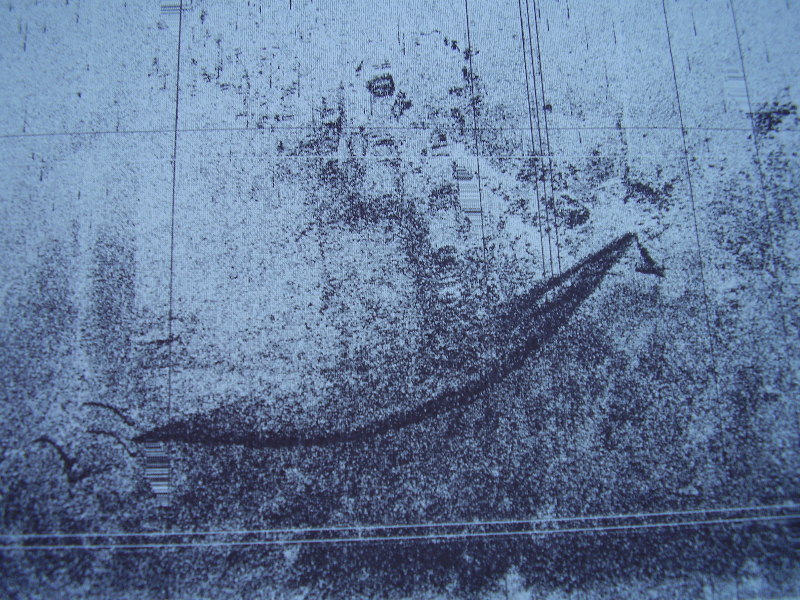
Figure 3.10: ADCP backscatter plot showing distinct return between 18m and 27m |
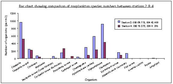
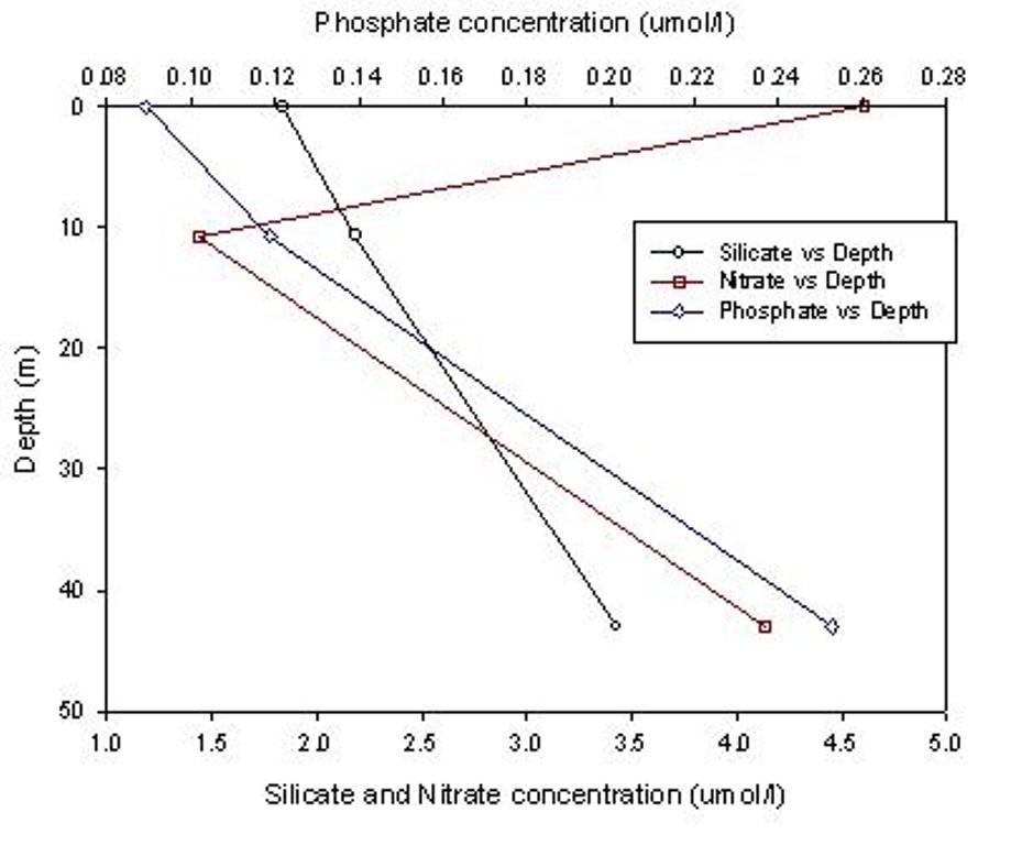
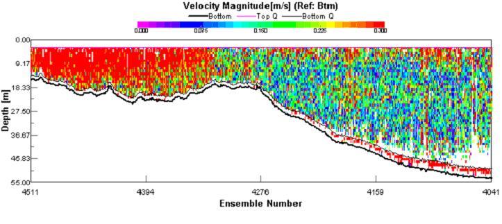
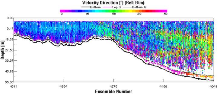
Date: 08/07/2006 Introduction: Using the Research Vessel Callista Group7 aims to observe the vertical mixing processes of the water column off Falmouth in order to understand how the functional properties and structure of plankton populations are affected both, directly and indirectly, by the water column’s properties. Weather conditions: 40mph winds, force 8 sea state, 70% cloud cover (sunny intervals) Methods: Four stations were sampled on Callista (see fig 3.1), the first station was Black Rock (050.08.318, 005.01.436). The other stations formed a transect, to the east, starting offshore and moving closer to the coast. The start of the transect was station 2, at 050 09 .115N, 004 43 .400W. The purpose of this transect was examine how the depth of the thermocline is affected in shallower water and to compare how the biological, chemical and physical parameters change approaching the shore. Due to weather warnings of 40mph winds, and a force 8 sea state we could not go as far offshore as we had previously planned for practicality and safety reasons. At each of the four stations we deployed the CTD and collected water samples with Niskin bottles. From these water samples, two oxygen samples were taken first, then samples for nutrients (phosphate and nitrate in one bottle, silica in another) and phytoplankton were also taken. The nutrient samples were filtered, and the filters were added to Acetone in test tubes and stored in the fridge. A closing zooplankton net was also deployed at each station, collecting zooplankton from different depth zones in the water column. Comparing stations 2 and 4 (figure 3.2), zooplankton species were counted and identified from vertical trawls done from a depth of 12m to the surface. Station 2 appears to have higher numbers of individuals with on average (taken from the sum of taxa in m3 divided by number of different taxa) a total of 246 individuals per m3 and with a total number of 135 per m3 for station 4. Copepods are seen to be a dominant species with 959 m-3 at station 2 and 516 m-3 at station 4. When worked out as a percentage of total number, Copepods made up approximately 25% of the samples from both stations. Cirripedia larvae (Barnacles) made up a higher percentage of station 4’s sample, with 13%, but only making up ~4% of the sample taken from station 2. Phytoplankton numbers were also analysed from 100ml seawater sample put into Lugol’s solution, and then counted under a microscope using a Sedgwick-Rafter chamber. At station 2, the total number of phytoplankton (approximated from counting 10 transects of 1 ml each) was estimated to be 26500 per l. Station 4 showed a lower value of around 18000 per l, with the sample being dominated by Nitzschia sp (figure 3.11), which make up approximately 38% of the sample. Rhizosolenia delicatula is the second most abundant species found at station 4, making up ~24%. Station 2 appears to be dominated by Rhizosolenia delicatula (figure 3.3), making up 27% of the sample, closely followed by Rhizosolenia alata with 23% of the sample. The highest chlorophyll concentrations (1.93ug/l and 1.89ug/l) in seawater were found at station 2 (Boris Johnson) at a depth of 10.7m. The next highest value (1.19ug/l) was sampled from a depth of 16m from station 3 (John McEnroe), with the lowest chlorophyll reading being found at station 3, sampled from the surface. Conclusion: The lowest Oxygen concentrations were found at Station 2 (Boris Johnson). This is also where the highest amounts of chlorophyll and zooplankton were found, indicating that this is the most productive region sampled, at 10.7m. The primary production here is balanced by the respiration of the zooplankton, causing the depletion of dissolved oxygen. The highest Phosphate values we found were collected from a depth of 43m at station ‘Boris Johnson’ 2, with a concentration of 0.342umol/l. The two lowest concentrations of phosphate found were both surface samples, one of which was taken at Boris Johnson station (0.089umol/l). The highest Silicate concentrations were found at Station ‘Maria Sharapova’ 4, with a concentration of 4.713umol/l sampled from a depth of 13m. The surface samples consistently had the lowest concentrations, ranging from 1.609 umol/l (John McEnroe) to 2.759 (Maria Sharapova), suggesting depletion possibly due to summer stratification (low wind shear). Nitrate concentrations were generally higher at the surface than at depth, with the exception of the data collected at station 2 (Boris Johnson) which showed a very high peak at the surface (perhaps an explanation for the high chlorophyll levels at station 2), and then another peak at a depth of 43m of nearly as high a concentration as at the surface. However, at a depth of 10.7m the nitrate concentration had significantly decreased (figure 3.6). The lowest O2 concentrations were found at station 2 (Boris Johnson) at a depth of 43m, with values of ~262 umol/l, with saturation of ~97.5 %. The highest O2 concentrations were found in the surface waters at station 3 (John McEnroe) with concentrations of 299.5 umol/l and saturation of 122.8 %. At all of the stations O2 concentrations were lowest at depth, increasing up to their maximum values in the surface waters. Conclusion: The lowest phosphate and silicate samples were all collected from the surface, this is because the water is stratified due to summer warming and a lack of storm mixing and therefore phosphate, which is ‘incorporated into many biological molecules, for example, nucleic acids, and adenosine di- and triphosphates (ADP and ATP)’ (Miller, 2005). The highest phosphate concentration was found at the deepest depth; 43m at station 2, this is below the euphotic depth which three times secchi depth (10.5m) indicates to be 31.5m. When the amount of mixing increases later in the year, the phosphate may be brought up to the surface while there is still enough light for primary production leading to a fall bloom. The phosphate concentrations may also be regenerated on biweekly spring tides and after summer storms (as with other nutrients depleted from surface waters and persisting at depth). The highest silicate samples were found at the station closest in to shore (Station 3, Maria Sharapova); this could be caused by groundwater runoff, but is more likely to be from death and settling out of diatoms after a spring bloom. The nitrate concentrations tended to be higher at the surface, which would, at first glance, appear to be in contradiction to the other nutrients. However, the land usage near this transect is mainly agricultural, with the majority being dairy farming, which means that the runoff will be high in nitrates. CTD: The CTD data we collected was not unusable (figure 3.7) due to a faulty cable giving us irregular data, i.e. giving a depth reading of over 1000m whilst we were actually in 25m of water. As we were the only group that went east, we do not have another group’s CTD data that we can look at to compare our other data with. This has meant that although we were planning to have a close look at the thermocline structure at different stations, this was very difficult to do, and we had to sample at approximate depths where we thought the data was fairly reliable. ADCP: This ADCP profile (figure 3.8) runs from deep water about 2 nautical miles offshore, up onto a shallower plateau that surrounds the headland at Dodman Point (050°13N, 004°43W). At the time that this profile was taken, the tide was on its flood cycle, resulting in a large tidal flow into the English Channel. This flow is exacerbated around the headland with strong mixing and an even higher velocity magnitude than a mile offshore. Using the Eastwards velocity and velocity direction profile (figure 3.9) it is possible to see how the prevailing SW wind and tide flow has caused the top layer of the sea to move much quicker than the rest of the body of water. In fact it is possible to see how, when offshore, the prevailing wind results in the water moving at an angle of 45° to the wind. Further down the water column the direction of water transport has rotated with depth, and so is effectively flowing against the direction of the water mass 25m above it. This is a good example of the Ekman transport downward spiral in action. In the backscatter plot (figure 3.10) from the same ADCP profile, there is a distinct return from the area between 18 and 27m water depth in the offshore region. This is caused by a difference in density reflecting some of the signal to the ADCP. Further into shallower water the tide pushes the pycnocline upwards, and this can be seen on the profile where the backscatter contour creeps upward. |
Figure 3.2: comparison of zooplankton diversity between stations 2 and 4 taken from 12m-surface using vertical net
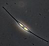
Figure 3.11: Nitzchia
species
Figure 3.3: Rhizosolenia delicatula (source: bornova.ege.edu.tr)
Figure 3.6: station 2 vertical profile of nutrient data taken at the surface, 10.7m and 43m depth
Figure 3.8: ADCP from near Dodman Point showing velocity magnitude in m/s
Figure 3.9: ADCP velocity direction profile showing Ekman transport downward spiral |
||||||||||||||||||||||||||||||||
|
4. Geophysics
|
 |
|
||||||||||||||||||||||||||||||||
|
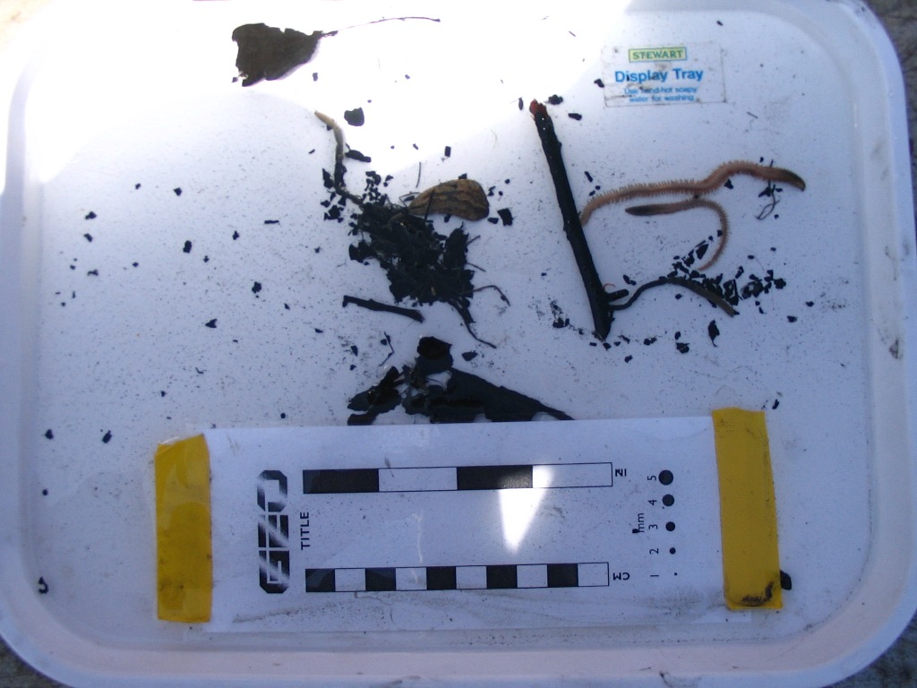
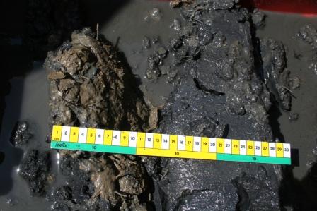
Figure 4.4: ragworms and detrital material from site 2
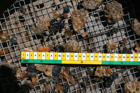
Figure 4.5: site 3, sediment (some bioclastic) filtered through 1cm mesh
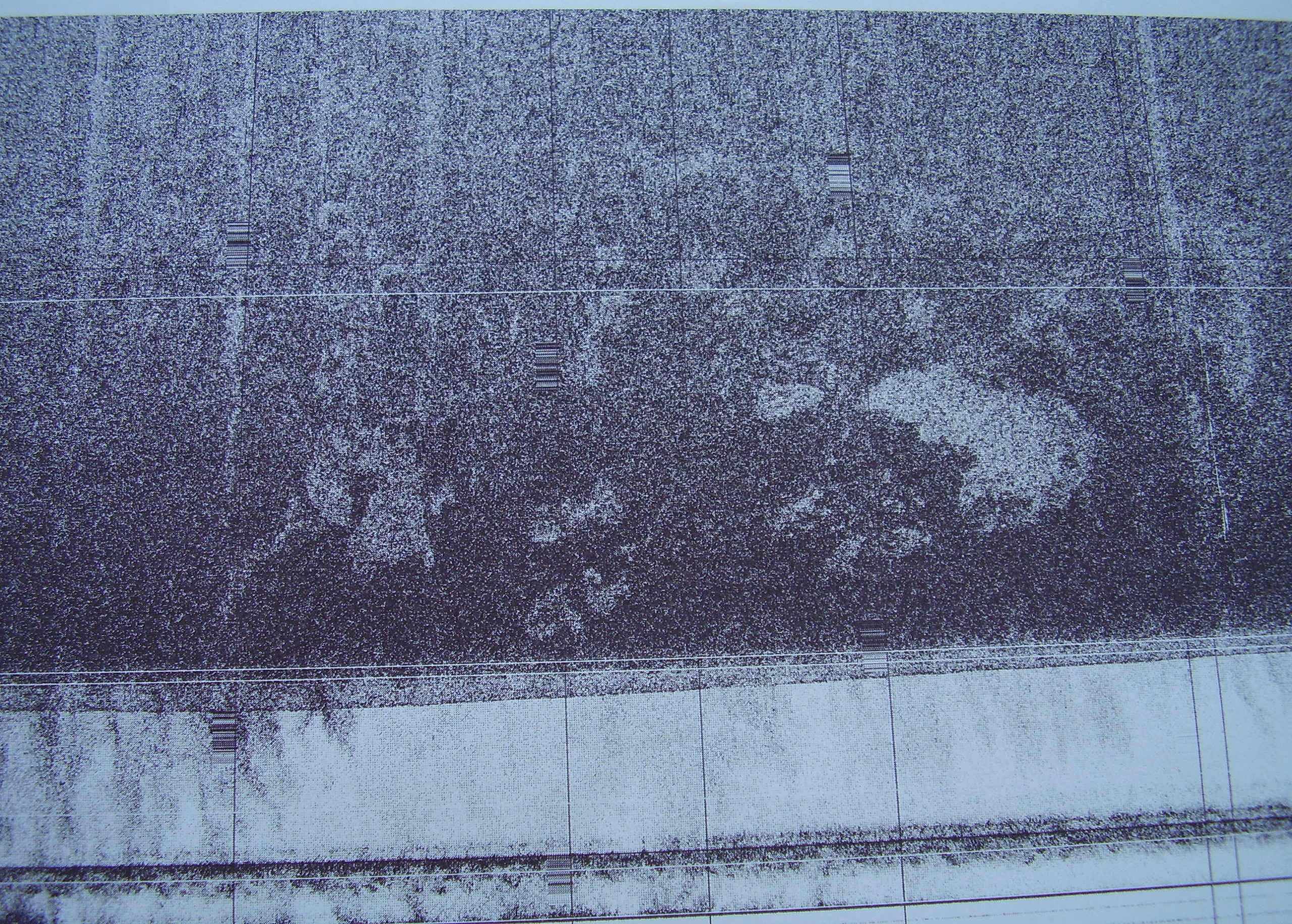
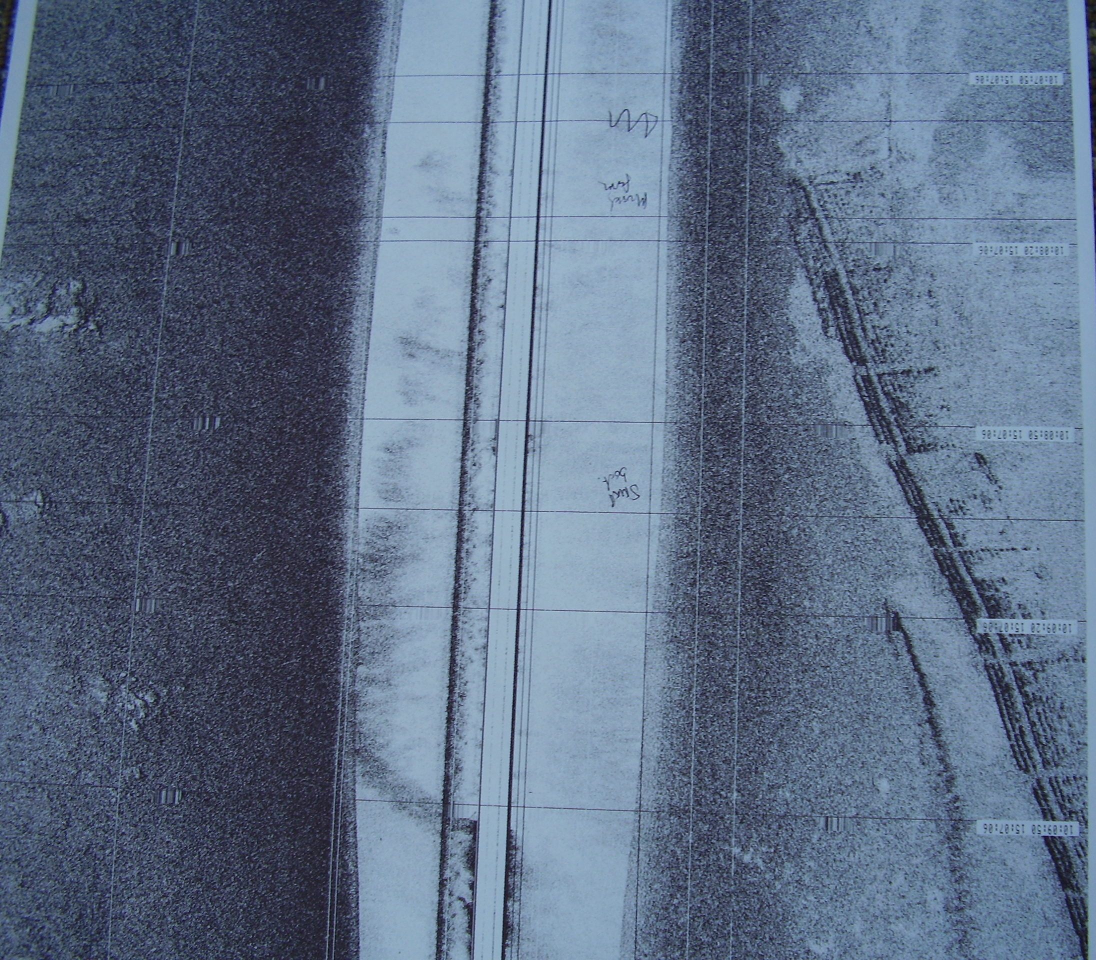
Figure 4.9: sidescan showing patches of fine clay sediment |
Date:
15/07/2006 Introduction: Aim: To survey the Fal estuary bed forms using the sidescan tow fish starting at the harbour channel (050o11.034N, 005o01.969W) and finishing at the most northern point possible taken into consideration the tidal conditions. High water was at 09:00 AST (GMT) at a height of 5.36m, allowing side scan to be surveyed up to 050o14.300N, 005o00.971W (Malpas Point). On the 15th of July group 7 carried out a geophysical practical using Grey Bear. We carried out a geophysical survey of the channel running up the Fal estuary using a side scan fish, which was towed behind the boat at a number of depths (depending on the depth of the estuary). While the tow was in the water a record of the position (longitude and longitude), course direction (degrees), time (AST) and a general description of surrounding environment (passing boats, distance from shoreline, mussel farm and other interesting features). On deck, one member of the group was observing the occurrence of boats, buoys, the shoreline, pipes, floating debris within 75m of either side of the boat. Due to the day of the week (Saturday) there were a large number of pleasure boats travelling up and down the estuary so a large number of washes were recorded within the side scan record. The sidescan fish was deployed at 09:16 AST in the harbour channel, recording continuously up the estuary to Malpas point (050o14 300N, 005o00 971W), with a continuous record of the estuary floor being printed out. Once the survey had been completed the printed record was studied and areas were noted which were of interest; suitable sites consist of changes in bed type or a point at which the sediment type was of a similar/same type to a large area of the other parts of the estuary floor. In total four grab samples were taken and an accurate identification of sediment type, and biology was noted and then the samples were returned into the water column when our observations were complete. Grab site 1:
Grab site 2:
Grab site 3:
Grab site 4:
Sidescan sonar interpretation: Higher up in the river the sediments are mainly dominated by fine-grained clays. Two grabs (1 and 2) were taken from this, it was found to be very anoxic, aside from a very thin oxic surface layer, black, and smelling slightly sulphurous. This is because of the detritus from nearby trees is decomposed by bacteria that use up all of the oxygen and have to use sulphur compounds to oxidize the organic matter. Another factor that could influence this is the runoff and sewage from higher up in the river. In previous chemical surveys of the estuary (by RIBs, and Bill Conway) high nitrate levels were found near Truro that were associated with higher phytoplankton numbers. This increase in nutrients can lead to a larger biomass in the water column and a greater amount of decomposition of this biomass. In the lower section of the estuary the sediments are mainly dominated by coarser material. This was found (from grabs 3 and 4) to be mainly bioclastic, made up of various sizes of broken shell fragments. However, no organisms were found in these samples, indicating that the shell fragments were deposited here from elsewhere. The presence of a mussel culture in the estuary shows that this lack of organisms is not caused by conditions in the water, it is more likely that the sediments are not suitable for them. Patches of coarser material can be seen higher up in the estuary, mainly located on the outside of bends, this is where the flow should be faster, allowing the suspension of the coarse material. After the bend, where the water flow decreases, the coarse material is deposited. In grab 4 the most coarse material was on top of the finer sediments, meaning that other sections that appear to be coarse from the sidescan may also just be on top of fine grained clays. This is what would have caused the patchy sections near the top of the estuary. References:
Admiralty (2006). Admiralty Leisure Charts
- SC5602: The West Country; Falmouth to Teignmouth. 7th Edition. |
Figure 4.2: ragworms from grab sample 2 taken from 050°13.8921N 005°01.0470W
Figure 4.3: juvenile crab from grab site 3
Figure 4.6: site 4 showing detrital material (right) and some bioclastic material (left)
Figure 4.7: sidescan print out showing ferry chains (right central)
Figure 4.8: sidescan showing mussel farm (right central)
Figure 4.10: sidescan
showing |