
Contents
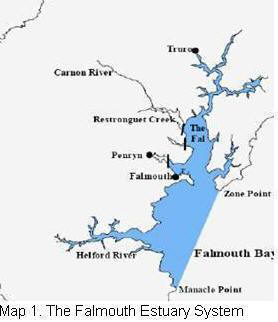
1. Introduction: Falmouth estuarine system
Estuaries are semi-enclosed coastal bodies of water having a free connection with the open sea, within which seawater is measurably diluted with freshwater derived from land drainage (Cameron and Pritchard, 1963). The Falmouth estuary, as the majority of its relatives in the UK coast formed after the rising sea levels, thousands of years ago when the last ice age came to an ends, drowning the existing river valleys, and creating the so-called Rias.
Falmouth and Helford estuaries to the east of Lizard Point are considered to be of national importance for their high diversity of marine habitats, communities, and species. Important species include the best-developed maerl bed outside Scotland and eelgrass. “The Mannacles”, a small group of rocks about two km offshore of Lizard Point support dense growths of sponges, hydroids, and sea squirts. To the west, the extremely exposed shores are often cited as classic examples of this shore type.
 Their emplacement on the South-West
region implies a series of considerations based on their underlying geology. The
study area in overall terms was at the southernmost extent of the ice sheets
during the last ice age. It is likely that ice cover and subsequent glacial
deposition was restricted to the northern coast down to the Isles of Scilly and
to one of the early periods of glaciation. Any deposits from this were covered
by later sea level rises and thus distributed across the area. Quaternary
deposits are, thus, limited in their extent and thickness (Evans et al.,
1990). In consequence, the seabed has generally a much lower thickness of sediments than areas such as the Irish Sea and North Sea, which
experienced considerable glacial deposition. Other than sediments derived by
glacial deposition, additional sources of sediment supply include deposition of
fine muds from the Severn estuary, the creation of carbonate rich material from
molluscs (biogenic material) and from the erosion of the solid bedrock geology
exposed on the sea floor. The seabed sediment thickness within the study area is
generally only in the order of a metre. Such low sediment thicknesses result in
either exposed bedrock or a very thin veneer of sediments over solid geology.
High tidal currents move the sediment to create bedforms such as mega-ripples
and sand waves, resulting in small areas of thicker sediments. Localised
thicknesses of material also occur along the northern coast where sediment has
in-filled deeper incisions created by the Severn River.
Their emplacement on the South-West
region implies a series of considerations based on their underlying geology. The
study area in overall terms was at the southernmost extent of the ice sheets
during the last ice age. It is likely that ice cover and subsequent glacial
deposition was restricted to the northern coast down to the Isles of Scilly and
to one of the early periods of glaciation. Any deposits from this were covered
by later sea level rises and thus distributed across the area. Quaternary
deposits are, thus, limited in their extent and thickness (Evans et al.,
1990). In consequence, the seabed has generally a much lower thickness of sediments than areas such as the Irish Sea and North Sea, which
experienced considerable glacial deposition. Other than sediments derived by
glacial deposition, additional sources of sediment supply include deposition of
fine muds from the Severn estuary, the creation of carbonate rich material from
molluscs (biogenic material) and from the erosion of the solid bedrock geology
exposed on the sea floor. The seabed sediment thickness within the study area is
generally only in the order of a metre. Such low sediment thicknesses result in
either exposed bedrock or a very thin veneer of sediments over solid geology.
High tidal currents move the sediment to create bedforms such as mega-ripples
and sand waves, resulting in small areas of thicker sediments. Localised
thicknesses of material also occur along the northern coast where sediment has
in-filled deeper incisions created by the Severn River.
The Fal estuary receives freshwater inputs not only from the main river, but also from additional ones on its sides, adding additional freshwater, hydrodynamic variability and complications to the system. Each particular river course and tributaries encompass a range of particular characteristics and components (from different physicochemical approaches), which add all together in the “Fal region”, modelling the system observed and challenging the oceanographic perspective of the environment.
Referring to the catchment and sedimentary environment in the Fal, both are a factor of its underlying geology (particularly determinant seems to be the Cammellis granite and metamorphic strata to the West (Hosking and Obial, 1966)). China clay wastes are also a source of input, having a major silting impact in the upper estuary and adjacent saltmarshes. The Falmouth region is well known by the mining industry as one of the most important areas nationally, and has been exploited as early as during the Bronze Age, with a peak of activity in the 19th century. Metalliferous deposits of Sn, Cu, Pb, Fe, and lesser amounts of As, W, U, and Ag, have been extracted, remobilising millions of tons of tailings, deposits, and sediments (generated by the mining activity and the minerals themselves). A good number of all these sediment-loaded waters have deposited at Restronguet Creek, making it the most metal polluted estuary in the UK (Bryan and Langston, 1992). Yet, there is existing data and therefore evidence, that substantial parts of these settled materials have been transported to other parts of the Fal by local currents and the dynamics of the system. This may have relocated the pollutant minerals over a wider area (less harmful), favouring a more benign situation. Large maerl beds are other key feature of the area, consisting of dead and live coralline algae. These algae are harvested and used for agricultural purposes, compensating for the low fertility of the surrounding soils.
The Helford River needs also consideration, given that comes into the Fal (at the end), contributing to the whole system. It is a drowned river valley or Ria, which catchment consists of sedimentary, Devonian carboniferous rock to the South and West. Contrary to the Fal, the Helford River lacks a mining industry complex in the vicinity, although there some indications of small-scale explorations and extractions. Cu, Zn, and Si seemed to be enriched, relative to standard values for the rest of the UK. This, however, does not represent a problem as in the case of Restronguet catchment.
2. Callista - Offshore sampling
Location and basic details
|
Date |
Lat. |
Long. |
Temp. |
Sal. |
Time |
Depth |
Tide |
Weather |
|
05/07/06 Day 186 |
50’ 10.736 N |
005’ 03.150 W |
17.73 C |
34.2 psu |
0810 GMT |
0.4 m |
HT = 1200 GMT LT = 1820 GMT |
8/8 cloud octants Wind ~ 3 m/s |
Introduction
 The western
English Channel tends to be thermally stratified during the summer months, due
to the increasing light and irradiance levels at this time of the year.
Stratification is dependent largely on several factors, such as water depth,
tidal dynamics and irradiance levels. Other factors affecting the structure at a
reduced scale are freshwater inputs and climate variability, all of this
affecting the structure of the water column.
The western
English Channel tends to be thermally stratified during the summer months, due
to the increasing light and irradiance levels at this time of the year.
Stratification is dependent largely on several factors, such as water depth,
tidal dynamics and irradiance levels. Other factors affecting the structure at a
reduced scale are freshwater inputs and climate variability, all of this
affecting the structure of the water column.
Changes in the vertical water column (mixing), affect physicochemical properties through the water masses, from the bottom of the euphotic zone, to the surface layers, where the different phytoplankton functional groups will develop (Kiorboe, 1993). Studies in stations off Plymouth Sound (L4 Station, near Eddy Stone Reef), indicate a balance between different factors behind the development of the plankton blooms. Indeed, light levels (avoiding development during the cold months), nutrient abundance (exhaustion avoiding growth during the summer months), cell capabilities in the water column (ability to move up and down and drift according to the local oceanographic parameters), grazing pressure (zooplankton feeding rate) and mortality (naturally occurring). The zooplanktonic community in turn, will be affected by other factors, such as the abundance of their prey (phytoplankton), distribution of their predators, natural mortality, capabilities of vertical migrations and horizontal movements following prey drifting. All this will lead to a patchiness in distribution of the zooplankton members both in space and time, which is a general characteristic of the water column.
Basic to the understanding of the vertical distribution of the planktonic community in the water column is the availability and rate of turn over and input of inorganic nutrients, which can foster growth in the nutrient-depleted waters experienced during the summer period. Nitrate and Silicate for diatoms are key modellers of the whole structure in the biological side, and may mix from below the thermocline in summer stormy events or sporadic turnover, triggering phytoplankton growth.
The aim of the experiment was to try to find a front structure outside the estuary, looking at the vertical parameters in the water column, as well as a basic analysis of the evolution of the thermocline when approaching the front. A very offshore sampling station was carried out, looking for the classical vertical structure in the water column, as well as other sampling station close to the mouth of the estuary as a general data point for all the working groups.
Materials and sampling procedure
Sampling effort and decisions about where to sample and the approach to take were discussed the previous day and at the harbour, prior to departure. A final decision was taken and the strategy adopted is shown on the map below:
- First station
at Black Rock (similar sampling location as other groups) to deploy all the
instrumentation and organize the team work properly.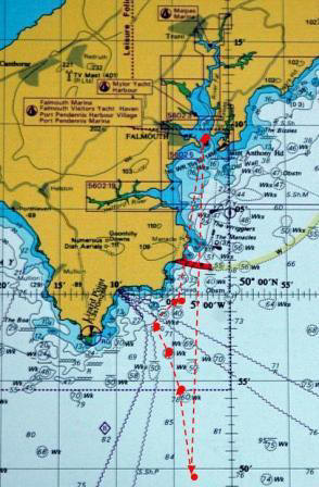
- Second station was taken the furthest offshore in order to try to find the classical situation in the water column of the western English Channel.
- Sampling effort after this point was backwards from the furthest point, trying to reach the front when approaching it.
- Offshore-onshore strategy approaching Lizard Point, in order to reach the front.
- Series of stations were carried out looking for a shallowing of the thermocline and its breakdown.
- CTD casts without any bottle sampling or closing plankton net effort were underway trying to find such a breakdown of the thermocline.
- At the point the correct vertical structure was found, bottle samples were taken, and plankton net was in place to monitor the community and physicochemical properties at these points.
- The last station was along the mixed side of the front.
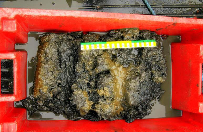
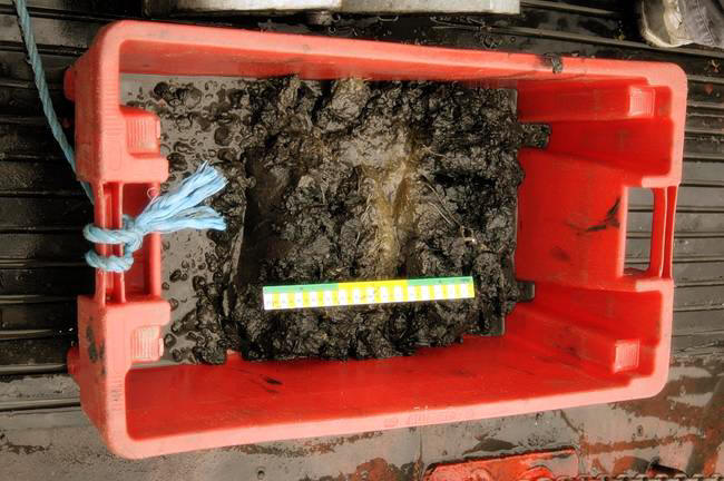
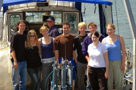
The team split in different groups to be able to tackle the work properly. Two members and the coordinator performed the deployment of the instrumentation; two other members did the chemistry and fetch the bottle samples when they were ready to collect on deck; the other two, worked inside with the ADCP and CTD computer screens, making sure the samples were taken at the correct places and the decision were right. They also did communicate with the crew staff deploying the CTD from the A-frame, ensuring the safety of all the working members. Pictures of the majority of the activities were taken in order to ensure a record of the different activities undertook.
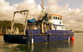
Vessel and Equipment Used
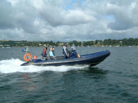
- Callista (35 ft) was used as the base boat and all the activity was carried out from there.
- A Secchi disk (all white) was used to determine the euphotic zone and simple data analysis used to determine the attenuation coefficient (k).
- An Acoustic
Doppler Current Profiler (ADCP) recording data between stations and at station
in order to infer current direction, velocity magnitude and backscatter (cue for
zooplankton abundance) was used.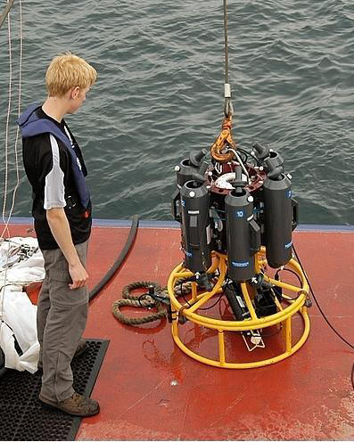
- A CTD (with light sensor, fluorometer, transmissometer, Niskin rosette) was used to collect samples at the required depths. The bottles were fired from inside after taking decisions when having a look to the CTD and ADCP screens. Priority was given to conspicuous thermoclines, chlorophyll peaks and zooplankton abundance when triggering a determinate bottle at a determinate depth.
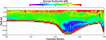
- A closing zooplankton net (60 cm diameter, 200 microns netting) to trap these organisms at the depths where the decisions were taken. This decision was taken after having a look at the CTD and ADCP data. Particular attention was paid to the “sandwich” effect of zooplankton feeding on phytoplankton from below and above, quickly reducing the size of the phytoplankton patch. Patchiness was also assumed to be at a premier in zooplankton distribution, and then they do not correlate well with phytoplankton records. Actually, zooplankton is not only affected by phytoplankton distribution and then the differences observed. Note however, that at Station 2 (i) for instance, a great phytoplankton record in the euphotic zone, was followed by remarkable zooplankton abundance just below as shown by the ADCP backscatter data and the following closing net bottles analysis at that particular vertical transect.
The Laboratory analysis
 - The work was
divided into morning session and afternoon session. The morning session aimed to
look at the biological aspects (phytoplankton and zooplankton taxonomy), and the
afternoon concentrated on the chemical aspects of the water samples
- The work was
divided into morning session and afternoon session. The morning session aimed to
look at the biological aspects (phytoplankton and zooplankton taxonomy), and the
afternoon concentrated on the chemical aspects of the water samples
- In the morning session the team split up in groups (half for phytoplankton and half for zooplankton), while in the afternoon session split up in pairs for the calculation of each parameter.
- Two members carried out each task, but nitrate, which was kindly analyzed by a member of staff after some trading (Mr. B. Dickie).
- After all the results were obtained, they were transferred to data files in order to be able to plot the findings against physical data from the boat.
2.1. Offshore Callista Results
ADCP analysis
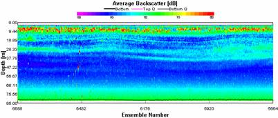
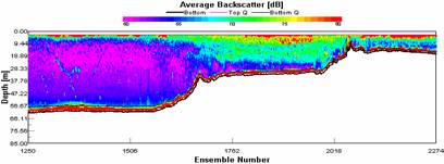
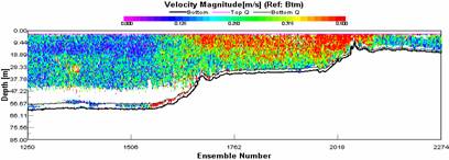
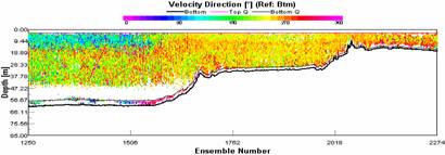
Current velocity and backscatter
 Water velocity and backscatter was
measured using an Acoustic Doppler Current Profiler (ADCP). It sends out pulses
of sound at a frequency of 1200 kHz. The volume of reflected sound or
backscatter can help determine the volume of suspended material in the water or
an estimation of the zooplanktonic community, given that the ADCP used the fact
that water moves, and the particles and organisms within the water move at the
same speed the water does. The Doppler shift of the sound is then used to
determine the speed of the water. The ADCP sends out normally three acoustic
pulses (the one installed on the hull of Callista bears four, the additional one
being used for calibration purposes) the speed determined from the return of
each of these is then used to calculate the velocity of the water column. This
instrument may be used aboard a moving vessel as the velocity is calculated
using the sea bed as the stationary reference point, and can also be employed
when the vessel is stationary.
Water velocity and backscatter was
measured using an Acoustic Doppler Current Profiler (ADCP). It sends out pulses
of sound at a frequency of 1200 kHz. The volume of reflected sound or
backscatter can help determine the volume of suspended material in the water or
an estimation of the zooplanktonic community, given that the ADCP used the fact
that water moves, and the particles and organisms within the water move at the
same speed the water does. The Doppler shift of the sound is then used to
determine the speed of the water. The ADCP sends out normally three acoustic
pulses (the one installed on the hull of Callista bears four, the additional one
being used for calibration purposes) the speed determined from the return of
each of these is then used to calculate the velocity of the water column. This
instrument may be used aboard a moving vessel as the velocity is calculated
using the sea bed as the stationary reference point, and can also be employed
when the vessel is stationary.

|

|


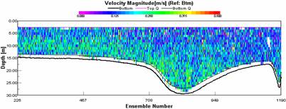
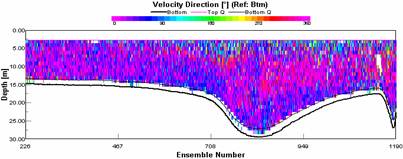
Fig 2.1.5. ADCP Graph to show velocity magnitude at station 2

|
Stations 4, 5 and 6 The next group of figures shows the ADCP data gained from a long recording with the ADCP which includes movements from site 3 to 4, 5 and 6 as we came back from offshore back into the headland. Current velocity is very low in the open ocean but as we move inshore the velocity increases. This may be due to the fact that we were returning in an opposite direction to the tide as it was an ebb tide. At 2595 m length the front clearly appears, the upwelling velocity figure also shows clear upwelling which is a result of the thermocline being near the surface, the backscatter in this area is very high as a result of phytoplankton being confined to the thermocline due to the lines of isopycnals, as well as nutrients being continually mixed in this region. A long line of foam was seen when passing the front, which suggests that upwelling is occurring, the fact that we were traveling fairly parallel inland to the foam line and another line of foam was not seen also supports that it’s an internal wave responsible for the upwelling not Langmuir circulation. The varying velocity in the ocean following the wave pattern is a result of the ocean trying to regain geostrophic balance as the wave disturbs the natural flow velocity in the ocean.
|


![]()
Secchi disk analysis
A Secchi disk was used to give an indication of depth of the euphotic zone, which is the theoretical lower limitation for plant growth in the water column (PAR; light limits the plan production, acting from above). The disk, which can vary in colour from completely white to black and white, is lowered into the water until the operator can no longer see a contrast between the black and white segments on the disk surface, this indicates the Secchi depth, which is then multiplied by a factor of three in order to get the roughly depth of the euphotic zone, its is said, where the phytoplankton is going to be able to grow successfully. The Secchi disk generally gives quite accurate results, however its limitations lie in that it assumes that the properties of the surface water are the same for the whole water column, and also relies on the human perception, which some times can be biased or can vary from observer to observer (thus, subjected to error variations).
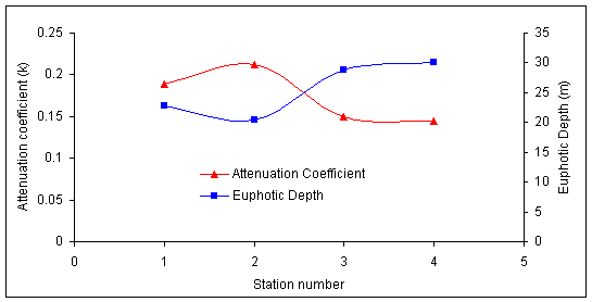
At Station 1, with a total depth of 15.4 meters, the euphotic zone (22.8 m) was well below this value, indicating that the whole water column was a suitable habitat for algal development, always depending on their species-specific light requirements and adaptability. The attenuation coefficient value reached 0.18 m-1, not being too high for the mouth of the estuary, where the water column was supposed to be well-mixed and the k value higher. Station 2 euphotic zone extended down to 20.4 meters, which again seemed strange for the 81 meters total depth at the furthest station. Water should be clearer than at the mouth of the estuary, and then the k value (0.21) should be smaller. The contrary is observed, and then, something may have gone on to cause this, or it could be a normal trend in the place. At Station 3, with a total depth of 44.7 meters, the euphotic zone seemed normal, higher than the two previous stations (28.8 meters), with a k value of 0.15, indicting not much turbidity or suspended matter in the water column. At Station 4, total depth was 61.6 meters, this seemed perfectly normal attaining the highest euphotic zone extension, and the smallest k value. Phytoplankton is then assumed to be able to grow down at the deepest for all the stations sampled. Again, few organic matter and suspended sediment present in water given the low attenuation coefficient calculated.

![]()
CTD, nutrient and plankton analysis
Station 2
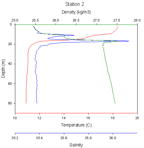 The
furthest station offshore showed a perfect situation related to the main
oceanographic parameters, with a roughly 7 degrees C change in temperature from
the surface layers to depth (18.4 to 10.88 degrees C). A constant temperature
gradient was reached at about 20 meters. The thermocline seemed to have a
gradient of roughly -1,7 (slope). This situation seemed obvious, given the
distance offshore the boat was located. Salinity considerations established a
constant trend throughout the water column, with salinity spikes at 10 and 16
meters through the thermocline due to the time lag between temperature and
conductivity. Density was developed with a small pycnocline, progressively
increasing with depth. At about 20 meters, increased down to 80 metes depth at a
steady pace, in a straight line fashion. The breakdown of this kind of
well-developed thermocline may take some time to be done, and seems optimum for
algal growth, as long as nutrients are in place. The whole structure seemed to
be extremely well stratified, and this could have an impact on the phytoplankton
development, given that they may be trapped in the surface water layers, and
then can fill up their light requirements, which is within their critical depth.
Phytoplankton growth is mainly a balance between light from above and nutrient
inputs from below. The situation is obviously not light limited (summer period),
but nutrient could already have been depleted in the previous spring and early
summer blooms. River runoff and inputs have been at a minimum for weeks, so only
vertical mixing from below the thermocline could replace the needed limiting
nutrients.
The
furthest station offshore showed a perfect situation related to the main
oceanographic parameters, with a roughly 7 degrees C change in temperature from
the surface layers to depth (18.4 to 10.88 degrees C). A constant temperature
gradient was reached at about 20 meters. The thermocline seemed to have a
gradient of roughly -1,7 (slope). This situation seemed obvious, given the
distance offshore the boat was located. Salinity considerations established a
constant trend throughout the water column, with salinity spikes at 10 and 16
meters through the thermocline due to the time lag between temperature and
conductivity. Density was developed with a small pycnocline, progressively
increasing with depth. At about 20 meters, increased down to 80 metes depth at a
steady pace, in a straight line fashion. The breakdown of this kind of
well-developed thermocline may take some time to be done, and seems optimum for
algal growth, as long as nutrients are in place. The whole structure seemed to
be extremely well stratified, and this could have an impact on the phytoplankton
development, given that they may be trapped in the surface water layers, and
then can fill up their light requirements, which is within their critical depth.
Phytoplankton growth is mainly a balance between light from above and nutrient
inputs from below. The situation is obviously not light limited (summer period),
but nutrient could already have been depleted in the previous spring and early
summer blooms. River runoff and inputs have been at a minimum for weeks, so only
vertical mixing from below the thermocline could replace the needed limiting
nutrients.
![]()
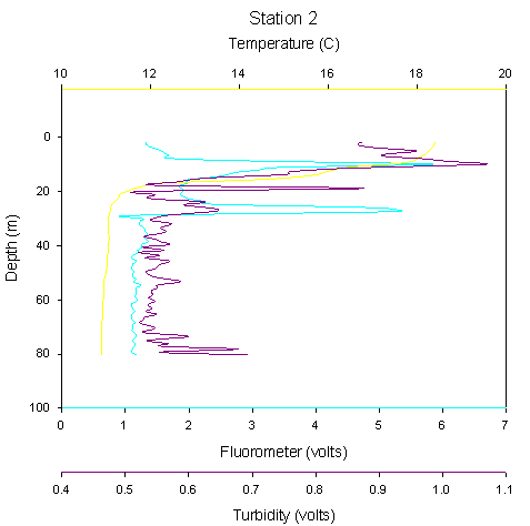 Chlorophyll analysis with fluorometer
revealed two biomass peaks at 9.9 meters (5.84 volts), and at 26.7 meters (5.28
volts). Deeper than this, chlorophyll evolved in a straight line fashion.
Curiously, having a look to the thermocline development, peaks of chlorophyll
stayed just above and below the thermocline. The internal wave activity
described previously in the ADCP, causes mixing in the pycnocline, which occurs
just above the thermocline, mixing occurring, bringing up nutrients within the
surface layers and thermocline. This could explain the chlorophyll peaks at two
different depths, the internal wave going through the thermocline, causing
mixing.
Chlorophyll analysis with fluorometer
revealed two biomass peaks at 9.9 meters (5.84 volts), and at 26.7 meters (5.28
volts). Deeper than this, chlorophyll evolved in a straight line fashion.
Curiously, having a look to the thermocline development, peaks of chlorophyll
stayed just above and below the thermocline. The internal wave activity
described previously in the ADCP, causes mixing in the pycnocline, which occurs
just above the thermocline, mixing occurring, bringing up nutrients within the
surface layers and thermocline. This could explain the chlorophyll peaks at two
different depths, the internal wave going through the thermocline, causing
mixing.
Diatoms abundance could explain the 26.6 meters peak (Rhizosolenia setigera and Rhizosolenia stolerforthii as the main representatives). Ciliates abundance at 9.9 meters could explain the peak, which is even higher than the deeper one (Karenia mikimotoi as the main representative). Turbidity acts as a good indicator of the mixing activity within the thermocline, which is due to diffusive processes from deeper water, and also due to mixing causing the internal wave along lines of isopycnals. This may trigger phytoplankton blooms, especially in the upper thermocline as it is not light limited. Turbidity peaks followed roughly chlorophyll ones in the vertical profile, indicating the mixing processes going on above and below the thermocline, which are though to be caused, among other factors by the internal wave formation, development and propagation.
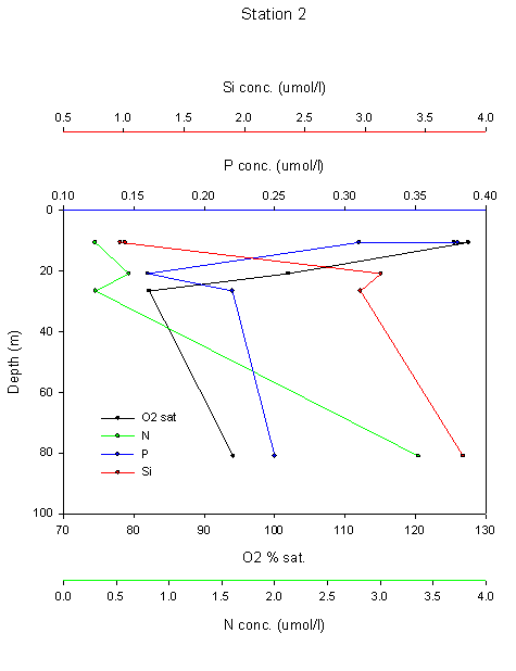 Nutrient
analysis revealed a nitrate depletion towards the surface layers, which is
expected, as all algal groups need it for growth. It is almost completely
depleted above and within the thermocline, and could be limiting down to 25
meters depth at some point, where it may be exhausted. It seems not to be the
case at the time the samples were taken, because the chlorophyll peaks still
show great biomass being in place. It inc
Nutrient
analysis revealed a nitrate depletion towards the surface layers, which is
expected, as all algal groups need it for growth. It is almost completely
depleted above and within the thermocline, and could be limiting down to 25
meters depth at some point, where it may be exhausted. It seems not to be the
case at the time the samples were taken, because the chlorophyll peaks still
show great biomass being in place. It inc![]() reases with depth as expected, below
the thermocline, where light limitation may be behind further phytoplankton
development. Phosphate disclosed similar results, being this nutrient depleted
towards the surface layers, but not exerting as much limitation as Nitrate.
Silicon was also depleted above and below the thermocline, down to a depth where
it started to increase, maybe because of the decrease in diatoms number, being
consumed by zooplanktivorous organisms and the poor conditions for their optimal
development present. However, it may be noted, that one of the main supplies of
Si is the riverine inputs, but as this station is far offshore, freshwater
influence may not be too marked. Nonetheless, freshwater is scarce at this time
of the year due to the lack of rain for weeks, which makes the rivers to
discharge low volumes of water. Below the thermocline, between 30 and 15 meters,
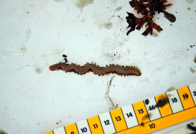
were the first closing net for zooplankton was deployed, the numbers obtained
were remarkable, indicating zooplanktonic activity feeding on the phytoplankton
activity observed. This was expected, as ADCP analysis also revealed high
backscatter levels at these depths, indicating zooplankton presence, just below
the phytoplankton. Hydromedusa, along with copepods and Decapods larva
constituted the bulk of the individuals. From 15 meters to the surface, the
zooplankton community was different from the deeper counterpart. Shallower,
well-stratified waters within and above the thermocline, teemed with Hydromedusa
and Decapods larva again, and new abundant members, as Echinoderm larva and
Copepod, all the groups with much fewer individuals than the deeper layers. This
may represent a vertical depth section, where zooplankton development is not
optimum, being this part well below the thermocline and well lit surface layers.
reases with depth as expected, below
the thermocline, where light limitation may be behind further phytoplankton
development. Phosphate disclosed similar results, being this nutrient depleted
towards the surface layers, but not exerting as much limitation as Nitrate.
Silicon was also depleted above and below the thermocline, down to a depth where
it started to increase, maybe because of the decrease in diatoms number, being
consumed by zooplanktivorous organisms and the poor conditions for their optimal
development present. However, it may be noted, that one of the main supplies of
Si is the riverine inputs, but as this station is far offshore, freshwater
influence may not be too marked. Nonetheless, freshwater is scarce at this time
of the year due to the lack of rain for weeks, which makes the rivers to
discharge low volumes of water. Below the thermocline, between 30 and 15 meters,
were the first closing net for zooplankton was deployed, the numbers obtained
were remarkable, indicating zooplanktonic activity feeding on the phytoplankton
activity observed. This was expected, as ADCP analysis also revealed high
backscatter levels at these depths, indicating zooplankton presence, just below
the phytoplankton. Hydromedusa, along with copepods and Decapods larva
constituted the bulk of the individuals. From 15 meters to the surface, the
zooplankton community was different from the deeper counterpart. Shallower,
well-stratified waters within and above the thermocline, teemed with Hydromedusa
and Decapods larva again, and new abundant members, as Echinoderm larva and
Copepod, all the groups with much fewer individuals than the deeper layers. This
may represent a vertical depth section, where zooplankton development is not
optimum, being this part well below the thermocline and well lit surface layers.
The phytoplankton-zooplankton vertical
distribution disclosed a c![]() urious four layers “sandwich” structure, which may
indicate some kind of patchy feeding strategy on the side of zooplankton. Above
the thermocline there was a layer with a chlorophyll peak, indicating
phytoplankton abundance, just below and within the thermocline, zooplankton
blooms were present as well. Below the thermocline another chlorophyll peak
indicated algal growth going on, and just below, as expected, zooplankton
bloomed. If this four layers “microsystem” was to be monitored for some time
continuously, the zooplankton will finally end up the phytoplankton bloom
development, and migrate somewhere else. The alga then, will have time again to
re-grow, provided they have enough nutrient being mixed from below, and positive
light levels from above (they also needed to be trapped at their optimum growth
depth).
urious four layers “sandwich” structure, which may
indicate some kind of patchy feeding strategy on the side of zooplankton. Above
the thermocline there was a layer with a chlorophyll peak, indicating
phytoplankton abundance, just below and within the thermocline, zooplankton
blooms were present as well. Below the thermocline another chlorophyll peak
indicated algal growth going on, and just below, as expected, zooplankton
bloomed. If this four layers “microsystem” was to be monitored for some time
continuously, the zooplankton will finally end up the phytoplankton bloom
development, and migrate somewhere else. The alga then, will have time again to
re-grow, provided they have enough nutrient being mixed from below, and positive
light levels from above (they also needed to be trapped at their optimum growth
depth).
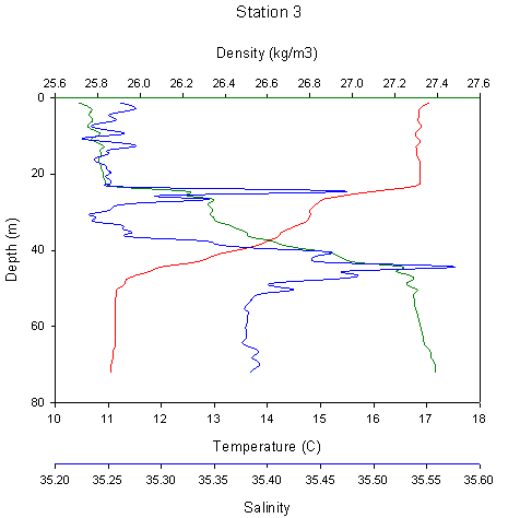
Station 3
Station 3 was sampled when heading backwards from the mightiest one offshore, in an attempt to reach the front structure, apparently present on the area. The thermocline started at 23.5 meters, ending down to 44.3 meters, with a temperature variation at around 6 degrees C, from 11 to 17 degrees C. The thermocline deepened since Station 2, but it was not as steep. This showed how the thermocline started to weaken, as the proximity to the front and to land decreased (increased mixing). Mixed conditions will be encountered further onshore, that will finally breakdown the oceanographic parameters observed at this station. On top of the thermocline (first 23.5 meters), it seemed to be warmed water layers with a temperature of about 16.8 degrees C. Salinity and density on that layer seemed also very stable, indicating a water mass almost free of any kind of turnover or disturbance at all. Phytoplankton could be trapped at that warmed, stratified water layer, productively blooming (commented later on). Salinity is fairly constant through the water column (change of 0.25), showing two spikes at 35.4 (24.5 meters) and 35.6 (44.37 meters). Density analysis revealed a pycnocline between 24 meters and 44 meters, showing the inverse of the thermocline development. Below this depth, it increased at a constant rate in a steep manner.
The fluorometry trend showed large increases in the thermocline, peaking when the turbidity peaked. This could be caused by the mixing up of nutrients, allowing phytoplankton to bloom successfully. Indeed, there were three consecutive chlorophyll peaks, starting at 26.5 meters, going down to 35.4 meters, being the last one at 44.36 meters. Yet, this chlorophyll peaks at such depths (especially the last one), seemed a bit odd, since the euphotic depth calculated with Secchi disk analysis revealed a euphotic depth of 28.8 meters at Station 3.
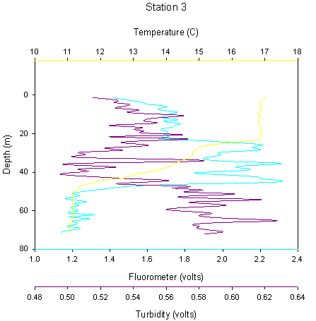
![]()
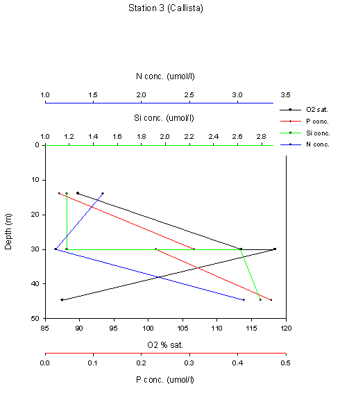
Nutrient
profiles and analysis revealed a depleted surface layer for all three ![]() nutrients,
increasing with depth. Nitrate decreased from the surface down to 30 meters,
corresponding with the phytoplankton biomass peak at such a depth. Phosphate is
depleted at the surface layers, increasing with depth, indicating that phosphate
is not a limiting factor for phytoplankton in this area. Silicon disclosed no
change down to 30 meters (low quantities), where it increased dramatically, and
then kept increasing progressively down to 45 meters. These conditions could
lead to think that diatoms may be successfully dominating the phytoplanktonic
community above and within the thermocline.
nutrients,
increasing with depth. Nitrate decreased from the surface down to 30 meters,
corresponding with the phytoplankton biomass peak at such a depth. Phosphate is
depleted at the surface layers, increasing with depth, indicating that phosphate
is not a limiting factor for phytoplankton in this area. Silicon disclosed no
change down to 30 meters (low quantities), where it increased dramatically, and
then kept increasing progressively down to 45 meters. These conditions could
lead to think that diatoms may be successfully dominating the phytoplanktonic
community above and within the thermocline.
Station 5
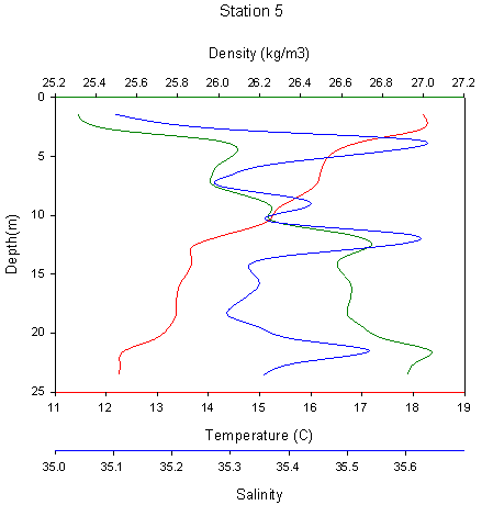 At
Station 5, the front was already reached and the sampling station was
established on the well-mixed site of the front, however as explained later on,
Station 6 is in the most conspicuous p
At
Station 5, the front was already reached and the sampling station was
established on the well-mixed site of the front, however as explained later on,
Station 6 is in the most conspicuous p![]() art (related to mixing) of the front. A
note on Station 4 relates to the fact, that its structure was mid-way between
Station 2/3 and 5, and then needs not much commenting.
art (related to mixing) of the front. A
note on Station 4 relates to the fact, that its structure was mid-way between
Station 2/3 and 5, and then needs not much commenting.
The temperature profile seemed to reflect a well-mixed structure with a very shallow, reduced thermocline developed at approximately 4 meters depth. There was a 6 degrees C change from the surface to 23.5 meters, but it followed an almost constant decrease down to roughly 13 meters, where the gradient increased. Stratification was only reached at the very surface if it existed at all, and the front impact was seen as the vertical breakdown of the thermocline along its structure.
Salinity showed there was not much variance and it reiterated the fact that the water column was well-mixed on the coastal mixed side of the front. Density increased fairly constantly with depth, reflecting the decrease in temperature down to 15 meters, beyond this point, the gradient increases down to the bottom.
There was a peak in chlorophyll at 6.5 meters representing the chlorophyll maximum (2.36 volts). Turbidity increased dramatically at the same time as chlorophyll did it but if having a look to the turbidity units increase, there is only a change of about 0.2 units, which is minimal. Turbidity measurements reflected the situation of the water column being well-mixed (Station 5 was close to the shore).
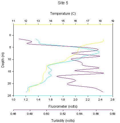
No sampling![]() effort was done at the chlorophyll maximum depth, so the phyto and zooplankton
present status could not be assessed. However, in a disturbed water column, in
the way it was seen in the profiles, the phytoplankton will not be trapped at
any particular depth, and they will drift with the water hydrodynamics.
Nutrients were not sampled, but it is assumed that if water is well mixed,
nutrient influx will be in place at all depths. In this situation, if water is
to get stratified, alga may find their optimum conditions to grow. This was
difficult to be reached at Station 5 due to its geographical situation at a
point where eddies caused among other factors by Lizards Point were at a
premier, and where a front developed, triggering at times increasing turnover of
the water column breaking down the thermocline (being this feature, among
others, a diagnostic characteristic of the system).
effort was done at the chlorophyll maximum depth, so the phyto and zooplankton
present status could not be assessed. However, in a disturbed water column, in
the way it was seen in the profiles, the phytoplankton will not be trapped at
any particular depth, and they will drift with the water hydrodynamics.
Nutrients were not sampled, but it is assumed that if water is well mixed,
nutrient influx will be in place at all depths. In this situation, if water is
to get stratified, alga may find their optimum conditions to grow. This was
difficult to be reached at Station 5 due to its geographical situation at a
point where eddies caused among other factors by Lizards Point were at a
premier, and where a front developed, triggering at times increasing turnover of
the water column breaking down the thermocline (being this feature, among
others, a diagnostic characteristic of the system).
Station 6
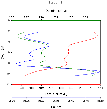
Station 6 was
the closest to Lizards Point, the shallowest, in the well-mixed side of the
front, and therefore a point
![]() where physical processes may model the
oceanographic environment. Temperature decreased with depth steadily, to about 8
meters, where there was a sharp decrease from 16.7 degrees C to 15.8 degrees C,
at the same depth that salinity decreased from 35.8 to 35.5. This was only a
slight salinity decrease, but enough to increase density and reduce mixing, thus
a sharper decrease in temperature. The thermocline was completely broken down,
illustrating the well-mixed side of the front, where the samples were taken.
Salinity and density mimic their profiles at almost all times in the profile.
where physical processes may model the
oceanographic environment. Temperature decreased with depth steadily, to about 8
meters, where there was a sharp decrease from 16.7 degrees C to 15.8 degrees C,
at the same depth that salinity decreased from 35.8 to 35.5. This was only a
slight salinity decrease, but enough to increase density and reduce mixing, thus
a sharper decrease in temperature. The thermocline was completely broken down,
illustrating the well-mixed side of the front, where the samples were taken.
Salinity and density mimic their profiles at almost all times in the profile.
Fluorometry showed one major peak at roughly 5 meters depth, having increased from 1.44 volts to 1.55 volts. This was also where turbidity peaked, possibly indicating a link between the two parameters. As the samples progressively moved from deeper stations to the shallow coastal ones, through the front, chlorophyll peaks shallow as well as a result of decreasing depth, increasing turbidity (higher dynamics in the system) mixing the whole thing up, avoiding enough light levels (PAR) to be available deeper in the water column.
With respect to nutrient concentrations, Station 6 showed a greater abundance of all nutrients, compared to the surface layers of the other stations. This may reflect the proximity of the land, the mouth of the estuary with freshwater inputs of all nutrients, and the well-mixed situation at this part of the front.
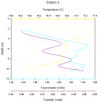
In this
well-mixed system, phytoplankton may bloom when transient stratification is
re-establ![]() ished or if they are not mixed below their optimum growth depth.
Theoretical considerations indicate mixed conditions should favour diatoms, in
detriment of flagellates and ciliates (Margalef, 1978). Indeed, when having a
look to phytoplankton abundance figures, diatoms dominate the system, probably
taking advantage of the present conditions, as well as the close situation of
the estuary mouth, where more silicon is expected present.
ished or if they are not mixed below their optimum growth depth.
Theoretical considerations indicate mixed conditions should favour diatoms, in
detriment of flagellates and ciliates (Margalef, 1978). Indeed, when having a
look to phytoplankton abundance figures, diatoms dominate the system, probably
taking advantage of the present conditions, as well as the close situation of
the estuary mouth, where more silicon is expected present.
Zooplankton analysis revealed a well populated area, with some variability between species, with typical coastal species present, which differ from the offshore ones, mainly in numbers, and in some cases in the taxonomic representatives in place.
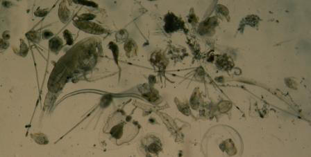
Phytoplankton analysis
Phytoplankton records for
four stations were sampled,
a brief comment on species
abundant and distribution is given. The possible interpretation for the results
obtained, and relations with nutrients and physical structure were given above.
Note that six stations were sampled, but at two of them, only CTD analysis was
carried out, and no bottle was triggered due to the lack of the searched picture
of the water column. At Station 1, Rhizosolenia stollerforti was the most
abundant species, followed by Chaetoceros sp. And then other
Rhizosolenia species were present at low numbers. At Station 2 (i),
Karenia mikimotoi w![]() as
t
as
t![]() he
most common one, followed by Rhizosolenia species and Ceratium
fucus. At this station was observed the highest zooplankton numbers, just
below and within the euphotic zone, probably preying upon some of these phyto
species. At Station 2 (ii) was observed
he
most common one, followed by Rhizosolenia species and Ceratium
fucus. At this station was observed the highest zooplankton numbers, just
below and within the euphotic zone, probably preying upon some of these phyto
species. At Station 2 (ii) was observed ![]() the
maximum variability in phyto species, ranging from Rhizosolenia species
to Karenia mikimotoi, Ceratium fucus and C.
tripos, Mesodinium rubren… At Station 6, again Karenia
mikimotoi was omnipresent, followed by Rhizosolenia
stollerforti, Ceratium and other species within Rhizosolenia
appeared.
the
maximum variability in phyto species, ranging from Rhizosolenia species
to Karenia mikimotoi, Ceratium fucus and C.
tripos, Mesodinium rubren… At Station 6, again Karenia
mikimotoi was omnipresent, followed by Rhizosolenia
stollerforti, Ceratium and other species within Rhizosolenia
appeared.
![]()

Zooplankton analysis
![]()
Zooplankton
records for the four stations sampled with a closing plankton net are shown here
with ![]() ba
ba![]() s
s![]() ic
comments on them. Note the variability in the dominant species between stations.
At Station 1,
ic
comments on them. Note the variability in the dominant species between stations.
At Station 1, ![]() Ctenophores
dominated the community, followed by Hydromedusa, which were omnipresent at all
stations. Copepods also turned up, being common at all samples as well. This
station was the one with more variability in groups, probably reflecting the
proximity of the mouth of the estuary and its benefits. At Station 2 (i),
Hydromedusa were the dominant group, followed by Decapod larva and Copepods.
Note that at Station 2 (i), there was high phytoplankton biomass present, and a
particular phytoplankton species preyed upon by copepods, which could have
determined the observations witnessed (but not necessary). At Station 2 (ii)
Hydromedusa dominated again, and Decapoda and Copepods were present. This
station was sampled from 15 m to the surface, and then it is observed less
amounts of zooplankton, contrary to the deeper sample, which showed up a high
quantity of zooplanktonic organisms. This could be explained as the zooplankton
been normally below the phyto comm
Ctenophores
dominated the community, followed by Hydromedusa, which were omnipresent at all
stations. Copepods also turned up, being common at all samples as well. This
station was the one with more variability in groups, probably reflecting the
proximity of the mouth of the estuary and its benefits. At Station 2 (i),
Hydromedusa were the dominant group, followed by Decapod larva and Copepods.
Note that at Station 2 (i), there was high phytoplankton biomass present, and a
particular phytoplankton species preyed upon by copepods, which could have
determined the observations witnessed (but not necessary). At Station 2 (ii)
Hydromedusa dominated again, and Decapoda and Copepods were present. This
station was sampled from 15 m to the surface, and then it is observed less
amounts of zooplankton, contrary to the deeper sample, which showed up a high
quantity of zooplanktonic organisms. This could be explained as the zooplankton
been normally below the phyto comm![]() unity, and not at
the same level as could be the case in the 15 m to surface sample. At Station 6,
at the well mixed of the front, the zooplankton representatives present was at
its highest. Copepods, Copepod nauplii, Decapod larva, Ctenophore, and even
Appendicularia representatives. Hydromedusa was again the dominant group.
unity, and not at
the same level as could be the case in the 15 m to surface sample. At Station 6,
at the well mixed of the front, the zooplankton representatives present was at
its highest. Copepods, Copepod nauplii, Decapod larva, Ctenophore, and even
Appendicularia representatives. Hydromedusa was again the dominant group.

A comparison between the phytoplankton and zooplankton records per station, indicates a fairly similar amount in both groups. At Station 1 and 6 there is less zooplankton present, while at Station 2, zooplankton took over the alga. Obviously, zooplankton biomass was always below phytoplankton one; this is to be expected, because from one trophic level to the next one, only 10 % organic matter is assimilated, and then much higher quantities of food are needed for zooplankton to make any capture worthwhile (do as many as possible). Other environmental and confounding variables may also be affecting zooplankton distribution versus phytoplankton abundance. Sampling procedures can also vias these kind of data manipulation, indicating a wrong or lower than expected abundance.

Location and basic details
|
Date |
Lat. |
Long. |
Temp. |
Sal. |
Time |
Depth |
Tide |
Weather |
|
08/07/06 189 |
50’ 10.772 N |
005’ 03.924 W |
17.23 C |
34.84 psu |
0835 GMT |
0.4 m |
HT = 1600 GMT LT = 1000 GMT |
5/8 cloud octants Wind ~ 3 m/s |
Introduction
 The
Fal Estuary bears two main river discharges from the Truro River and Tresilian
River, having multiple channels with middle areas of remarkable depth (10 to 30
meters), getting shallower when heading to the head of the rivers that flow into
it. Tributaries discharge into them in the form of smaller rivers, streams or
freshwater inputs into creeks. Creeks vary in size from a few tens of meters
(i.e., Channals Creek, Lamouth Creek and Tolcarne Creek, all near the lower
limit of the middle reaches) to some hundreds of meters (i.e., Restonguet Creek
and Mylor Creek towards the mouth of the estuary. They can be regarded as
mesocosmic areas, where microenvironments can be easily created such as in the
case of lagoons. In particular, some of the isolated ones may present different
tidal and physicochemical parameters than the adjacent settings, and the very
shallow parts may develop extremely conditions, challenging the growth of the
organisms inhabiting such areas. Some relative narrow channels near the rivers
mouth appear to present deep elongated areas up to 10/15 meters above chart
datum, which make them interesting zones for physicochemical and biological
analysis due to their importance and persistence during the low tides, getting
even deeper at high tide.
The
Fal Estuary bears two main river discharges from the Truro River and Tresilian
River, having multiple channels with middle areas of remarkable depth (10 to 30
meters), getting shallower when heading to the head of the rivers that flow into
it. Tributaries discharge into them in the form of smaller rivers, streams or
freshwater inputs into creeks. Creeks vary in size from a few tens of meters
(i.e., Channals Creek, Lamouth Creek and Tolcarne Creek, all near the lower
limit of the middle reaches) to some hundreds of meters (i.e., Restonguet Creek
and Mylor Creek towards the mouth of the estuary. They can be regarded as
mesocosmic areas, where microenvironments can be easily created such as in the
case of lagoons. In particular, some of the isolated ones may present different
tidal and physicochemical parameters than the adjacent settings, and the very
shallow parts may develop extremely conditions, challenging the growth of the
organisms inhabiting such areas. Some relative narrow channels near the rivers
mouth appear to present deep elongated areas up to 10/15 meters above chart
datum, which make them interesting zones for physicochemical and biological
analysis due to their importance and persistence during the low tides, getting
even deeper at high tide.
Changes in the vertical structure of the water column (mixing) affect physicochemical properties through the water masses, from the bottom of the euphotic zone (within the estuary limits it will be deeper than the total depth the majority of the time) to the surface. In the estuary channels, always bearing in mind tidal currents and other sources of disturbance (temporal or continuous), such as stormy events or flooding, the water column remains well mixed the majority of the time, making phytoplankton life a challenge at the deeper parts (increased turbidity). Only in sheltered areas, where disturbance is not at a premier, can a thermocline develop, which will not last for long. The thermocline development and its duration will be an oversimplified factor of the depth at which it may have formed and the source of the disturbance that could break it down and its intensity (if the thermocline is to be formed at all).
Salinity changes along the length of the estuarine system, from the mouth to the head, from the tributaries to the creeks, are of major importance for the development of the whole system. Monitoring these changes from the mouth-inshore or vice versa, can help to understand in an oversimplified way the dynamics of the system. Freshwater inputs can be roughly tracked from sampling effort undertaken with progressive samples took along the long of the estuary, monitoring drops in salinity every one or two units. However, in special circumstances, like the ones encountered in the Fal estuary at particular times during the tidal period (Group 5 situation), a units drop in salinity does not to seem to be the correct sampling procedure approach. The reason may be that with the incoming tide, and mainly because of the minimum freshwater inputs at this time of the year (lack of rain for weeks), the system does not develop as expected for such an estuary. This lack of freshwater makes the salinity variations in the middle and upper reaches very unpredictable. This means that it can be encountered situations such as 27.7 psu salinity measurements at one point (Tresillian River), and a 32.2 psu further up the estuary, where lower salinity is supposed to be present.
 Basic
to the understanding of the vertical distribution of the planktonic community in
the water column is the availability and rate of turn over and input of
inorganic nutrients, which can foster growth in the nutrient-depleted waters
experienced during the summer period. The inshore estuary system, approaching
the middle and upper reaches may be well-supplied with nutrients from different
inputs. Silicate may come from natural inputs from the land drainage and rocks
(underlying geology in the Fal mainly composed of granite and china clays
minerals). Nitrates and Phosphates may be derived from agricultural run-off,
activity well-developed around the Fal region, catchment, and adjacent areas
(agricultural lands are fertilized with derivates from coralline algae found in
the estuary; the maerl, which enhances crop production, and is directly harvest
within the estuary limits by determinate companies). Anthropogenic inputs from
populated areas close to the estuary borders may also increase this nutrients
abundance and phytoplankton blooms could be in place under the right
circumstances. Nitrate and Silicate for diatoms are key modellers of the whole
structure in the biological side, and may be added at a basic level from the
factors described above. Not noted in this analysis, may be the tube pipes
discharging these pollutants and organically/inorganically enriched waters, and
other sources of run-off, such as when the adjacent populated areas are washed
by rain and the waters drains down to the estuary carrying all the chemical,
particles and substances present on roads and humane infrastructures
Basic
to the understanding of the vertical distribution of the planktonic community in
the water column is the availability and rate of turn over and input of
inorganic nutrients, which can foster growth in the nutrient-depleted waters
experienced during the summer period. The inshore estuary system, approaching
the middle and upper reaches may be well-supplied with nutrients from different
inputs. Silicate may come from natural inputs from the land drainage and rocks
(underlying geology in the Fal mainly composed of granite and china clays
minerals). Nitrates and Phosphates may be derived from agricultural run-off,
activity well-developed around the Fal region, catchment, and adjacent areas
(agricultural lands are fertilized with derivates from coralline algae found in
the estuary; the maerl, which enhances crop production, and is directly harvest
within the estuary limits by determinate companies). Anthropogenic inputs from
populated areas close to the estuary borders may also increase this nutrients
abundance and phytoplankton blooms could be in place under the right
circumstances. Nitrate and Silicate for diatoms are key modellers of the whole
structure in the biological side, and may be added at a basic level from the
factors described above. Not noted in this analysis, may be the tube pipes
discharging these pollutants and organically/inorganically enriched waters, and
other sources of run-off, such as when the adjacent populated areas are washed
by rain and the waters drains down to the estuary carrying all the chemical,
particles and substances present on roads and humane infrastructures
The aim of the experiment aimed to discover and describe by the first time the physicochemical and biological environment at some of the remote parts of the Fal system (creeks, tributaries, and narrow estuarine channels). Other parts of the estuary were also sampled in order to gain general knowledge. The two main rivers (Truro River and Tresilian River), discharging freshwater into the estuary were sampled for both chemistry and biological parameters in order to establish any difference in their properties. One of the two rivers could discharge more freshwater than the other, and this could affect the settings in different ways.
Materials and sampling procedure
Sampling effort and decisions about where to sample and the approach to take were discussed the previous day and at the harbour, prior to departure. A final decision could not be taken until being in situ due to the dynamic variability of the system. Tidal tables and graphs to work out the available water level for sampling at complicate places, such as creeks and shallow sandy banks were monitored prior to departure and decisions were made. The sampling effort can be roughly described as follows and seen on the track map below:
- First station to make sure everything worked properly but with no further regard to analysis, given that it was taken at Mylor Harbour.
- A second station for analysis at
Turnaware Point just passed the main point where the channel getting inputs from
Truro River and Tresillian River, goes into the lower reaches of the Fal. Note
that a vertical profile was not taken at this point (too when sampling
backwards).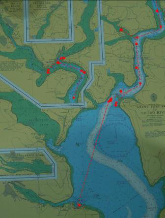
- Navigate all the way up to Malpas because the tide was still low and needed to wait it to flood a bit more. Samples were taken at Malpas (Station 3), and both boats meet to discuss the strategy, emphasising the need of in situ decisions to be able to monitor the situation properly.
- After samples were taken at Malpas, and decisions made, each boat aimed to sample a channel of the two rivers joining at Malpas. The Tresillian River part was sample as Station 4 and the Truro River as Station 5. The reason for this division of the task was to be able to compare the physicochemical environment between both rivers, which could be influenced by lower freshwater inputs.
- Sample procedure from these stations down was backwards, working against the tide. Station 6 took place at Woodbury Point, and Station 7 at Pontoon. These two stations were based on the Truro River.
- Down the Pontoon, on the right side, a creek baptized “Seal Creek” by the team due to a Harbour Seal feeding on a mullet, was sampled and constituted Station 8.
- Station 9 was Smuggler’s Cottage, close to the creeks analyzed as Station 10 (Cowlands and Lamouth Creek). Creeks as stated somewhere previously were analyzed regarding to find microenvironments development and special features of the creeks.
- Station 11 was Mussel Beds, near a mussel farm. Such a particular place may be influenced by the feeding and excreting activities of the mussels. More oxygen should be consumed near those places, and more organic matter present at the sea floor (consequence of pseudofaeces rejected when feeding, and organic material excreted by the mussels), consuming more oxygen. Water clarity was not analyzed with the materials available, but it is known to be very clean water near the mussel beds. Phytoplankton samples were also taken, in order to monitor any phytoplankton anomaly due to the mussel’s bed presence. A zooplankton tow was carried out in order to monitor the impact and the net was deployed I joint collaboration between the two boats.
- Station 12 was close to the same point were Station 2 was recorded. It aimed to monitor any tidal change due to the incoming tide, and also a vertical profile was performed.
Vertical profiles were taken at Station 7 (Pontoon), Station 9 (Smuggler’s Cottage), Station 11 (Mussel Beds), and Station 12 (Turnaware Point)The decisions about the points where these stations should be sampled was based on depth checking in the chart, making sure there was enough depth to carry out vertical profiles at several depths in the water column. An analysis of these vertical profiles may reveal a change in structure of the Truro River channel (all stations within the Truro extension), given that all four stations were taken almost consecutive in the same river section. Some physicochemical structure variability could be in place due to the inputs from some creeks along the section analyzed.
The team split in two groups (to boats) to be able to tackle the work properly. There was a main coordinator in one of the boats, who had the last decision, always having open communication via VHF with the other boat to jointly coordinate the efforts. In this way, double samples around the same area were avoided, and the work aimed to cover as much key estuary parts as possible. At times, one boat did one part of the sampling, and the other completed it with vertical profiles, so complementation, rather than overlapping on the sampling effort was feasible.
The technical instrumentation and use was as follows:
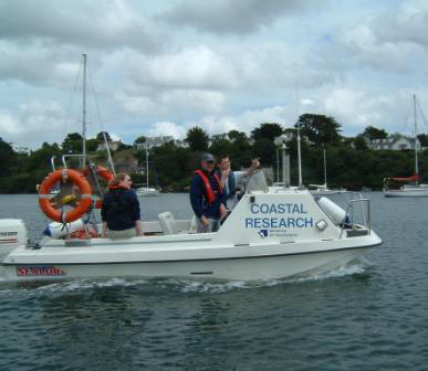
- Coastal Research and Ocean Adventure were used as boats and all the activity was carried out from those.
- A GO-flow bottle with releasing ends was used to sample for oxygen, and it was manually deployed into the water.
- A Secchi disk (white and black) was used to determine the euphotic zone and simple data analysis used to determine the attenuation coefficient (k). At the majority of the sites, but probably at the very deep ones, the theoretical euphotic zone was below the bottom maximum depth. A measuring tape was used to estimate the length of the rope from a notch toe the Secchi disk.
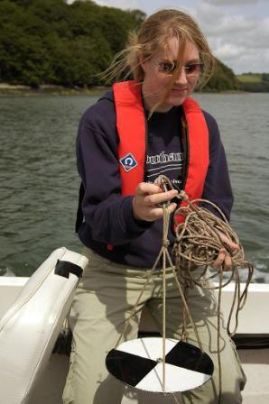
- A YSI 600 QS Multiprobe (as seen
in picture) was used
at each boat to monitor surface oceanographic parameters as well as sample
vertical profiles. Temperature, salinity, dissolved oxygen, and pH was recorded
from the probe.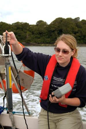
- An anemometer was used to monitor wind speed, and direction was roughly estimated manually.
- Plankton net, 200 microns net and 49.5 cm diameter, was used to collect zooplankton samples near the surface waters. A current meter was placed at the mouth of the net.
- A normal plastic bottle was manually dropped aside and a sample taken for different parameters analysis.
- Nutrient bottles for Nitrate ad Phosphate (crystal), and Silicate (plastic) were used to store water samples.
- Plastic tubes with acetone were used to store filters from the syringe when analysing chlorophyll, after the water was placed into nutrient bottles. The chlorophyll samples were placed into a container with a ice pack to keep them cold.
- Crystal bottles for oxygen were used, and a soft pipe used to transfer the water from the GO-flow bottle to the crystal bottle.
- Filters for chlorophyll were replaced in their appropriate plastic cover after each use, to be ready for the next sampling station. Two people were in charge of the chemical sampling manipulation and storage, while the others did the physical sapling part.
The laboratory work proceeded as follows:
- There was a timetable change in the chemical analysis due to some kind of problem, and while another group analyzed our chemical data, we analyzed their biological one.
- The work was therefore not split up as usually into pairs. Division into two groups proceeded, and while one aimed to analyze the zooplankton data, the other did the same with the phytoplankton bottles.
- Data was transferred into spreadsheets and logbook for further processing and analysis.
RIBs results and discussion
Nutrients in estuaries: a short overview
The riverine input of dissolved inorganic nitrogen and phosphorus to the ocean system is obviously of great importance in a discussion of the interactions of these compounds in the estuarine and adjacent coastal zones. However, the evaluation of the fluxes is complicated by the facts that there may be large seasonal fluctuations and that human activities have largely disturbed the natural fluxes. Except for dissolved silicon, the concentration of the nutrients observed in freshwater are extremely variable ranging from 0.4 to 60 µmoles litre-1 for phosphate and from 3 to 800 µmoles litre-1 for total dissolved inorganic nitrogen. These extreme compositional differences mainly reflect the influence of human activities.
The estuarine system is characterized by profound changes in the chemical properties of the water masses and usually by high biological activities, both of which significantly affect the speciation of the elements and transfer to the adjacent coastal zones. This is particularly true in the case of nutrients and organic matter.
Relating to nitrogen, the three main processes that modify its speciation in aquatic systems (nitrification, denitrification, and biological uptake), are commonly very active in estuarine systems and may significantly affect the transfer of nitrogen to the adjacent coastal waters and to the atmosphere, in the case of denitrification. The source of nitrate is essentially related to leaching of soil and to surface run-off. The use of fertilizers has considerably increased the concentration of nitrate carried by rivers. On the other hand, the presence of anthropogenic NH4+ is more directly related to domestic waste water discharges. As the estuarine zone is often heavily populated, high concentrations of ammonia are encountered, and organic phosphorus occurs mainly as orthophosphate in natural waters. In polluted estuaries receiving untreated domestic waste water, polyphosphates may represent a significant portion of the inorganic dissolved phosphate. Processes affecting the behavior of phosphate in estuaries are, however, very complex and probably not entirely identified and certainly not sufficiently understood
Silicon is, after phosphorus and nitrogen, the most common nutrient that limits the magnitude of the primary production in coastal and freshwater ecosystems. Recently, the Si cycle and its importance in several subdisciplines of limnology and oceanography has undergone some re-evaluation. The importance of Si as one of the nutrients governing the global total primary production of the world’s oceans and possibly the drawdown of carbon dioxide has been emphasized. Further, the dissolution of biogenic silica (i.e., diatoms) has clearly been under-estimated in many areas of the world. The interactions between Si and other elements, particularly P, at particle surfaces and its consequences is also an area of research which has received comparatively little attention until lately. Despite its comparative lack of complexity, or perhaps because of it, there are thus still several aspects of the silicon cycle which are insufficiently known. Silicon dioxide is the most abundant component of the earth crust present as well in igneous rocks than in sedimentary and metamorphic rocks. When exposed at the surface of the continents to water and wind, the silicates are submitted to weathering leading to dissolution and erosion. The chemical weathering contributes roughly to 50% of the dissolved fraction of fresh water. Dissolved silica, as undissociated silicic acid SiO4H4, represents a dominant species in river water, besides bicarbonate. In addition, most of the suspended matter carried by rivers is constituted by quartz of silicates, mainly clays minerals, resulting from the physical erosion of weathering products.
Horizontal structure
Nutrients
The strategy adopted to sample the horizontal distribution and structure related to nutrients, was not the appropriate to find low salinity values (high values anyways due to low river water inputs), and compare them to the nutrient concentrations. The methodology established, tried to sample remote places, such as creeks, and interesting areas, where some kind of phenomena could be noticed. Some typical horizontal changes with salinity were sampled, and added to the data collected by Bill Conway. 0 salinity and nutrient values were collected by Brian Dickie, and added to the original data sets for comparison, and evaluation of the likely Theoretical Dilution Lines, between which the nutrient concentrations could fit (above, in the middle or below), assessing the estuary situation. The general trend can be observed, as deviation from the TDL, but more accurate changes can only be assessed with a plot for the salinity range where the data was collected (not predicting the situation in the upper estuary reaches). A note of the Fal and Truro River, when analyzing the available data, relates to the fact that there Truro River was the focus of the analysis during the survey, and that the lower reaches of the Fal are the continuation of the data from the Truro River. This means that the majority of the data points come from Truro River, but some at high salinities are just at the confluence of Truro and Fal River or a bit onto the Fal River.
Silicon
The multiple TDL analysis seemed to fit quite
well with the scarce data available (no data from Bill Conway), and for all the
five rivers, the Si concentrations found were between the steepest and the
plainest TDL. This represented the range of concentrations in which Si can be
found in the Fal system (indication of the variance). Variability between rivers
was found, being the Kennel River, the one with lowest Si concentrations at the
mouth, and the Fal the one with the highest. These differences in 0 salinities
Si concentrations may reflect the underlying geology of each particular riverine
basin, as well as its particular inputs from natural sources, anthropogenic
continuous/diffusive points and other unknown sources. Si is expected to be
removed by diatoms along the estuary, decreasing its concentration near the
estuary mouth, but there is no data available to probe so in the upper and
middle reaches. In addition, more factors can influence in one or other way Si
removal apart from diatoms. What it is certain, is that freshwater
concentrations are always higher than seawater ones, given that the river
courses are key transporters of this inorganic nutrient.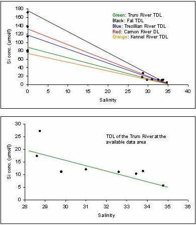
The situation assessed in a kind of detail was related to the Truro River (green line) in the range of salinities available. Taking a first simplistic approach, Si at salinity 0 at the mouth of the river was 81.2 umol/l, while at salinity 28.6, which is the second value available, the Si concentration was 17.32 umol/l. Obviously there is a decrease towards the seawater end member, which could be caused by diatoms, depending on blooming activity (if there is one at all), the state of this bloom and other confounding variables. Si however, tends to be conservative in estuaries during a good part of the year (especially winter months), and only during the spring bloom, and some summer events, its concentration may be lowered. This could generate non-conservative behavior at times.
There seems to be some removal from salinities 28.6 to 34.78, where existing data is available, especially between 28.6 and 31. This is supported by the phytoplankton analysis (Stations 5 to 8 in the 28.6 31 salinity range), where high numbers of diatoms were present (Nitzchia longissima, Rhizosolenia delicatula, Thalassiosira rotula, Rhizosolenia setigera). They probably have influenced the Si behavior lowering the concentration to 5.6 umol/l at the most seawater salinity. Indeed, when approaching the seawater end member there is a drop in concentration from 27.19 umol/l to 17.32 for salinity 28.74 to 28.6 (which seems strange, and should be treated with caution), and then from 17.32 umol/l to 11.14 at salinity 29.79. As stated, high diatom numbers were recorded, and may explain this sudden drops.
![]()
![]()
A chlorophyll analysis in the horizontal structure of the estuary also backs up the previous hypothesis. Chlorophyll relation to salinity changes in the salinity interval monitored for Si disclosed high values at 29.79 salinity (11.60 ug/l), decreasing to 9.7 ug/l at 30.99, which does not seem to be particularly marked (suggesting great abundance of diatoms as shown in the phytoplankton plots cell counting). Chlorophyll seemed much lower at 32 salinities, as shown in the Si plots, where its concentration was greatly reduced, not allowing diatoms to keep growing.
Nitrate
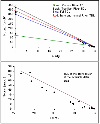 The
multiple TDL fitted well the data in the interval for the five river basins,
again with some variability, but not as marked as in the Si case. Only at the
Carnon River, the hypothetical TDL seemed to start at lower concentrations than
the rest (140 umol/l, versus a 350-420 umol/l range for the rest)), and its
steepness was not too marked. Nitrate is the most limiting nutrient at sea, but
is well abundant in freshwater, as shown in at the other four rivers. It may be
the particular situation of the Carnon River, which will need further
investigation in order to ascertain the causes of such lower starting values at
salinity 0. Nitrate is removed along all river basins from the freshwater member
to the seawater member. Again, the removal is particularly accentuated at all
rivers, but at the Carnon River. This indicates the fact that all phytoplankton
functional groups need nitrate for growing, and then it is a biolimiting
nutrient that when lacking limits alga development.
The
multiple TDL fitted well the data in the interval for the five river basins,
again with some variability, but not as marked as in the Si case. Only at the
Carnon River, the hypothetical TDL seemed to start at lower concentrations than
the rest (140 umol/l, versus a 350-420 umol/l range for the rest)), and its
steepness was not too marked. Nitrate is the most limiting nutrient at sea, but
is well abundant in freshwater, as shown in at the other four rivers. It may be
the particular situation of the Carnon River, which will need further
investigation in order to ascertain the causes of such lower starting values at
salinity 0. Nitrate is removed along all river basins from the freshwater member
to the seawater member. Again, the removal is particularly accentuated at all
rivers, but at the Carnon River. This indicates the fact that all phytoplankton
functional groups need nitrate for growing, and then it is a biolimiting
nutrient that when lacking limits alga development.
The particular situation assessed at Truro River revealed a conservative behavior of nitrate along its course, down to the confluence with the Fal. Some stations sampled in the Fal also showed conservative behavior closed to the seawater end member. It is known that the Fal Estuary is well supplied with nitrates (Parr et al., 1999) from different sources: agricultural (25-49 %), sewage treatment works (3-13 %), atmospheric deposition (2-6 %), nitrogen fixation (< 5 %). All these factors add together to create an environment, where nitrate is extremely well supplied, and then conservative behavior ensues, as supported by the data points.
In the 27.7-35.1 salinity range removal does not seem to be in place, despite of a good number of algal groups populating the water. At 34-35 salinity values, nitrate is almost depleted to 0 concentrations, and it could be argued to be exerting limitation on phytoplankton growth, which does not seem the case having a look to the cell counts for those stations.
Phosphate
The TDL did not fitted as well as in the other
station for phosphate. The data points obtained seemed to be out of the range
for any theoretical dilution line for the five rivers. Only some of the samples
at high salinities did fit. This situation indicated a net input of phosphate
from different sources along the estuary and its riverine catchment and
tributaries. The Kennel and Carnon River were at the extremes, showing high (3.6
umol/l) and low (0.5 umol/l) concentrations respectively at 0 salinities.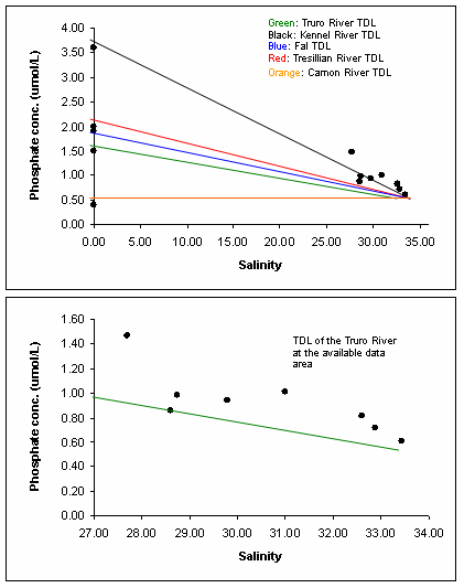 In between, the other three rivers reached between 1.5 and 2umol/l
concentrations at 0 salinities. This different 0 salinities variance reflects
the different input sources; variability along the estuary also reflects point
and diffusive sources present.
In between, the other three rivers reached between 1.5 and 2umol/l
concentrations at 0 salinities. This different 0 salinities variance reflects
the different input sources; variability along the estuary also reflects point
and diffusive sources present.
Addition of phosphate to the different rivers and tributaries could come from many sources, which should be further investigated and assessed. However, taking the data from Parr et al., 1999, a simplistic picture of the current situation can be drawn. Agricultural sources (3-49 %), sewage treatment works (26-62 %), atmospheric deposition (1.5-1.8 %) represent the main inputs and could explained the enrichment observed. For all rivers there seems to be extremely high inputs added to the system. Particularly, for the Carnon River, the inputs are the highest, probably reflecting and extra addition of phosphate to its catchment system.
The Truro River situation seemed to be one the most affected by external inputs, as reflected by the deviations from the theoretical dilution line after having a 0 salinity value in place. There seemed not to be a complete depletion of phosphate at high salinities (reduced phosphate concentrations), which means it is not limiting algal growth.

Nutrients and chlorophyll analysis
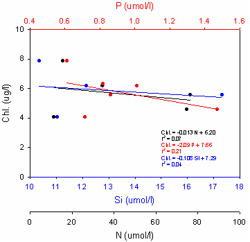 Regression
analysis was undertaken, trying to relate nutrients present and chlorophyll
values, in order to show a depletion of nutrients at higher chlorophyll levels.
Some stations disclosed peaks in chlorophyll, which may be lower in nutrients,
and then this could be analyzed with correlation trends. Each nutrient will be
depleted in a different way at each station depending on the phytoplankton
functional group present, abundance, and other unknown variables.
Regression
analysis was undertaken, trying to relate nutrients present and chlorophyll
values, in order to show a depletion of nutrients at higher chlorophyll levels.
Some stations disclosed peaks in chlorophyll, which may be lower in nutrients,
and then this could be analyzed with correlation trends. Each nutrient will be
depleted in a different way at each station depending on the phytoplankton
functional group present, abundance, and other unknown variables.
Negative correlations are seen for the three nutrients, but none of them seemed to be statistically significant (not tested because license for available statistical package was expired), with r2 values of 0.07 (nitrate), 0.21 (phosphate), and 0.04 (silicon). The negative trend found is what to be expected if the system is behaving normal, but even though it is so, more data points are needed to asses the current situation. Phosphate seemed to explain the variability in chlorophyll more than the other nutrients, and this could either be caused by vias on data (few data points), due to random variability or because the functional groups present may need phosphate more than he other inorganic nutrients.
Figure 3.1.4. Graph showing the correlations between chlorophyll and the three main nutrients
Vertical structure
Station 7 (Pontoon – furthest upstream)
Salinity increased as expected with depth; at 0 meters, salinity was 33.4 and at a depth of 7 meters salinity increased to 34.8. Temperature, oxygen saturation and pH decreased with depth. At 0 meters, temperature was 18.1 °C, O2 % saturation was 167 % and pH was 8.54. At 7 meters, temperature decreased to 17 °C, O2 % saturation was 138% and pH was 8.42. The Secchi disk depth was 2.01 meters, giving a euphotic depth of 6.03 meters.
Station 9 (Smugglers cottage)
Salinity increased with depth; at 1 meter salinity was 38.7 and at 13 meters it increased to 35.2. Temperature, oxygen saturation and pH decreased with depth. At 1 meter, the temperature maximum was 18.4 °C and the minimum was 15.7 °C at a depth of 13 meters. The O2 and pH maximum occurred at 2 meters and were 164% and 8.56 respectively; their minimum values occurred at 13 meters and were 114% and 8.43. The Secchi disk depth was 2.14 meters, which gives a euphotic zone depth of 6.42 meters.
Station 11 (Mussel Beds)
Only temperature and salinity profiles were measured. Temperature decreased with depth; from 17.8 C at surface to 16.4 C at 9 meters. Salinity increased with depth, 33.8 at surface to 34.8 at 9 meters. The Secchi disk depth was 2.05 meters which gives a euphotic depth of 6.15 meters.
Station 12 (Turnaware bar)
Salinity increased from 34.8 at surface to 35.1 at 7.46 meters. Temperature, oxygen saturation and pH increased between 0 and 1 meters, then decreased with depth. Temperature, O2 saturation and pH maximum all occurred at 1 meter with 17.2 °C, 174% and 8.54 respectively. Minimums all occurred at 7.46 meters with a temperature of 15.36 °C, O2 saturation of 145% and a pH of 8.45. The Secchi disk depth was 2.90 meters, which gives a euphotic depth of 8.7 meters.
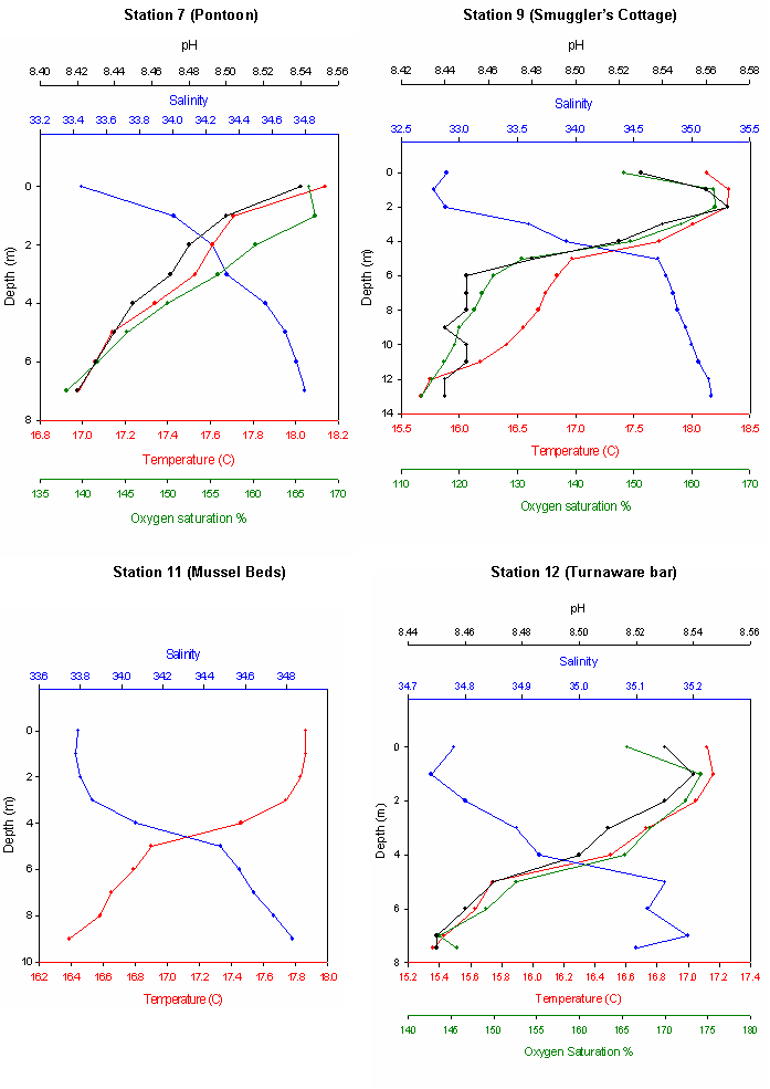
Discussion
At all stations, cold, dense, saline water seemed to flow up the estuary with the incoming tidal cycle. Warmer, less saline freshwater flows down the estuary from Truro and Tresillian riverine inputs. Reduced values in salinity were not remarkable, indicating some freshwater diluted with the incoming salt water, but not reaching extremely low values as expected from the river input dynamics.
The temperature profile at Station 7 revealed a well-mixed water column, where a thermocline was not developed. However, this is normally a transient situation, which depends on the total depth, hydrodynamics of the system and heat from above. The vertical profile for salinity was quite unexpected at the furthest station upstream; less than a factor of two was the increase in salinity with depth. It can be pointed out in this way, that there is no fresh water layer on top the seawater at this station, reflecting the lack of a great riverine flow going into the estuary. Dissolved oxygen followed a normal trend with depth, being higher at the surface, where the present algal community may be generating more, and then it will be supersaturated. Down to the bottom, oxygen levels decreased, but they were never undersaturated. The pH also decreased with depth as expected. A taxonomic algal analysis at this station, revealed a diatom-dominated environment (Nitzchia longissima, Rhizosolenia delicatula), where other functional groups were in low numbers or even absent.
At Station 9, the profiling effort seemed also to follow a normal trend. Temperature, dissolved oxygen and pH decreased all with depth, almost mimicking their trend lines. A slight thermocline developed at the surface, which will be rapidly dissipated by mixing processes. At peak in pH and dissolved oxygen was observed at about 1.5 meters, probably caused by a chlorophyll peak (no data for it), indicating the presence of positive algal growth going on. Salinity developed a small halocline (change in a factor of 2 in 4 meters), stabilizing at about 4 meters, increasing steadily down to 13 meters. A fresher water layer could be in place, but the incoming tide may have diluted it to a great extent.
At Station 11 only temperature and salinity values were recorded (cannot point out a reason why the others were not recorded). The trends shown were normal, with the development of a small thermocline and halocline respectively down to a bout 4 meters depth
Station 12 was not very different from Station 9, showing mimicking lines of temperature, dissolved oxygen and pH. However, in this case, the thermocline was broken down, and there was a peak of both oxygen and pH very near to the surface. Salinity did not show a recognizable halocline, and the presence of freshwater could not be founded.
Maximums of dissolved oxygen concentration occur generally around 1 meter depth, indicating high rates of photosynthesis (possible phytoplankton bloom). This may be so because of the mixing nature of the estuarine system, not allowing light to penetrate deep enough for positive algal development at depth. The surface water layers may be the most optimum for their growth, and then the data found. The oxygen saturation decreased with depth below 1 meter, showing an increase in the consumption of oxygen. Therefore, with depth respiration rate exceeds photosynthesis rate. The oxygen saturation levels at stations 7, 9 and 12 were very high; therefore it is suspected that the probe used was not calibrated properly. However, the trends produced by the values appear to be characteristic of an estuary, even if freshwater is not in place as it is supposed.
The pH decreased due to increasing concentration of CO2 with depth throughout the water column. Respiration rates exceeded photosynthesis rates therefore CO2 production exceeds its consumption. CO2 combines with seawater to produce bicarbonate and hydrogen ions
CO2 + H2O à HCO3 + H+
Increased concentration of CO2 results in increased production of H+, which decreases with depth.
Station 9 showed a more stratified vertical profile when compared with the other stations, which could be due to it being the deepest station, whereas at the shallower and lower water volume station (7) the lower saltwater is mixed with the upper freshwater.
Planktonic community
Phytoplankton
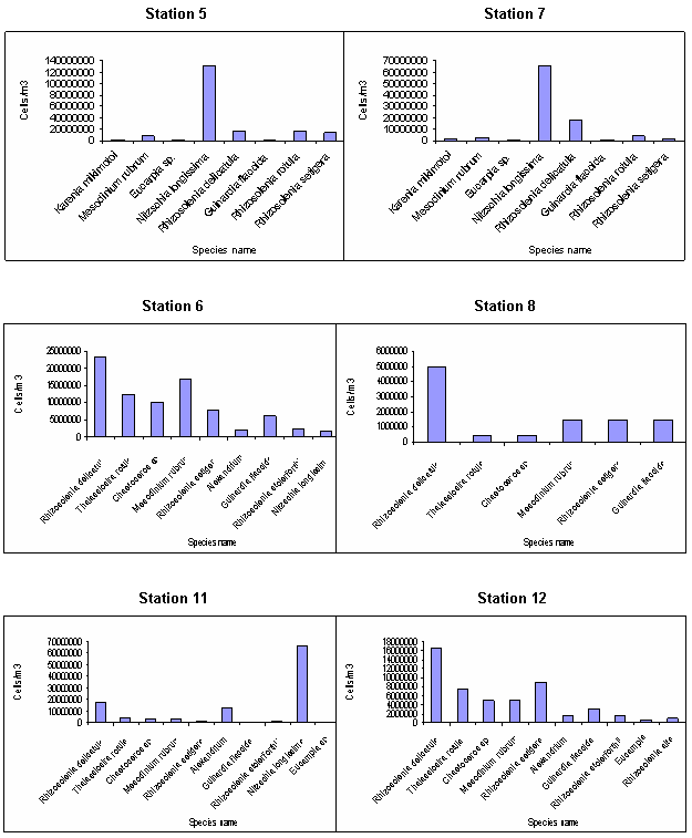 The
phytoplanktonic community can evolve in both spatial and temporal terms.
Spatially, it will be distributed along the estuary and riverine channels,
depending on the different nutrient availabilities, salinity and temperature
constraints and other confounding variables. Temporally, alga will be mainly
modeled by tidal cycles, riverine fluxes and other sources of variability
subjected to all kinds of modification. A particular population encountered at a
time at one salinity range, may change its position either upstream or
downstream (tidal change), following the salinity change, the temperature, the
nutrients availability, or in the majority of the cases a multifactorial
balance.
The
phytoplanktonic community can evolve in both spatial and temporal terms.
Spatially, it will be distributed along the estuary and riverine channels,
depending on the different nutrient availabilities, salinity and temperature
constraints and other confounding variables. Temporally, alga will be mainly
modeled by tidal cycles, riverine fluxes and other sources of variability
subjected to all kinds of modification. A particular population encountered at a
time at one salinity range, may change its position either upstream or
downstream (tidal change), following the salinity change, the temperature, the
nutrients availability, or in the majority of the cases a multifactorial
balance.
In general terms, diatoms dominated the upper reaches of the estuary in the Truro River, with the following species disclosing remarkable numbers: Nitzchia longissima, Rhizosolenia delicatula, Thalassiosira rotula, and Rhizosolenia setigera. Progressive heading to more salty waters, the functional groups started to change, with ciliate representatives in place. The main representatives were the following: Mesodinium rubrum and Alexandrium. At the last station (12), near the main Fal estuarine system, the most diverse community was found, with representatives of all the functional groups present upstream, and some of more open waters. However, diatoms dominate the situation by far, illustrating the suitable habitat that the brackish waters represent for some representative species.
A special consideration was taken at Station 11 (Mussel Beds), in order to analyze if the mussels were causing any impact on the phytoplanktonic community, and which repercussion could this have on zooplankton (discussed in the next section). The phytoplanktonic community seemed to be reduced in the samples taken close to the mussel bed. Only Rhizosolenia delicatula and Nitzchia longissima were abundant, with some Alexandrium in place. Mussel’s diet could not be assessed, but it is suspected that they mainly feed on bacteria-level organisms, microphytoplankton, and organic matter. They could also filter some higher phytoplanktonic organisms present, and explain the situation present. Nonetheless, mussels are known to clean the waters where they live, reducing organic matter, and this could also explain the lack of many phytoplankton species, even if the station is situated close to the Fal system, where more variability is expected (as in Station 12).
Zooplankton
A single zooplankton trawl was carried out along the mussel beds structure, at a roughly distance of 10 meters from the main mariculture setting (security distance). Total depth was 17.2 meters, water temperature 17.86 degrees C and 33.79 for salinity. A lower than normal oxygen concentration value was found in the area (67.7%); indeed the lowest for the whole estuarine system (in available samples). Mussels consume oxygen for metabolic purposes, and the tidal cycle may not have replaced the water masses present yet. However, these temporarily reduced oxygen levels may be changed as soon as the tide re-flushes, eliminating the hypothesis of the mussels affecting the oxygen. A deeper insight into the question leads to think that below mussel beds high organic material may accumulate, and thus, high bacterial activity levels may be in place. High organic decomposition levels may draw down more oxygen from the water column and water adjacent to the bottom. When this low oxygen water emigrates across the water column, it may lower the oxygen concentration if the organic material on the bottom covers a remarkable area. This lack of oxygen can explain to a certain extent the zooplankton distribution, but also mussels filtering activity may avoid the area to be suitable for their development. Copepods living on the top meter or so, dominated the community, and few representatives of any other group were abundant. Only Cirripedia larvas were found along with copepods. Other functional groups may not find this area suitable for living, or it may be a temporal situation, and at other tidal state, the community will evolve and change representatives.
Location and basic details
1st transect
2nd transect
Site
Main channel near the water skiing area
Site
Falmouth Banks
Date
12/07/06
Date
12/07/06
Lat. start
50’ 12.180 N
Lat. start
50’ 10.000 N
Long. start
005’ 02.500 W
Long. start
005’ 02.100 W
Lat. end
50’ 11.350 N
Lat. end
50’ 09.500 N
Long. end
005’ 02.800 W
Long. end
005’ 03.010 W
Boat speed
4.3 knots
Boat speed
4.5 knots
Tide
LT = 01:00 0.83 m 13:20 0.83 m
HT = 06:50 5.08 m 19:10 5.48 m
Comments
Data on boats passing and buoys encountered was recorded in order to infer any misrepresentation of the benthic picture picked up by Sidescan
Comments
Data on boats passing and buoys encountered was recorded in order to infer any misrepresentation of the benthic picture picked up by Sidescan
Introduction
Sidescan; a brief overview
Sidescan sonar reveals useful information about sea floor composition and properties by taking advantage of the different sound absorbing and reflecting characteristics of the different materials present at the bottom. Some types of benthic components, such as metals or recently extruded volcanic rock, are very efficient at reflecting acoustic pulses. Clay and silt, however, do not reflect sound so well. Strong reflectors generate strong echoes, while weak reflectors create weaker echoes. Knowing these characteristics, the strength of acoustic returns can be used to examine the composition of the sea floor. Combining information provided by a Sidescan sonar with the depth information from a range-finding sonar, can be a powerful tool for examining the characteristics of the ocean bottom.
Sidescan sonar works mainly in the same way as a conventional depth sounding sonar. Pulses are transmitted by a transmitter using a projector and hydrophones receive echoes of those pulses from the ocean floor and pass them to a receiver system. Where Sidescan sonar differs from a depth-sounding system is in the way it processes these returning signals.
The transmitter of the single-beam echo sounder produces an acoustic pulse, or ping, which is transferred into the water by the projector. The ping expands as a spherical wave from its source, striking the sea floor at the point closest to the projector source. The ping is then reflected in a returning spherical wave pulse, part of which is detected by the hydrophone. The time lag between the transmission of the ping and the reception of its echo is used to compute the range to the sea floor.
Sidescan sonar can receive the echoes from the bottom using two hydrophones, each set up to receive the returns from one side of the ship’s survey track. In reality, instead of one projector and two hydrophone arrays, two line arrays are used as transducers. One transmits a fan beam towards the port side and then listens to its returns, and the other does the same on the starboard side. When a pulse front first strikes the bottom below the survey vessel, an echo returns from only the one point of intersection. Later, however, the pulse front intersects the bottom at two points, one on each side of the ship. The echoes from these two points would occur simultaneously, and a single hydrophone system would have no way of distinguishing between them. If, however, two separate hydrophones each record the echoes from only one side of the ship, there would be no such confusion. The name “Sidescan” is used for historical reasons, because these sonars were originally built to be sensitive to echo returns from bottom locations on either “side” of a survey ship, instead of directly below as was the case for a traditional single-beam depth-sounder. With the advent of multibeam sonars, which map both depth and Sidescan across a swath of the bottom, the distinction inherent in this name has become less meaningful.
Each trace recorded by Sidescan is converted into a series of gray shades on a plotting device (paper, and a computer image adjacent can be obtained). The shade of gray is determined by the amplitude (white corresponding to high amplitude, black to low amplitude, or vice-versa). The port and starboard traces are plotted next to and facing each other so that the ship’s track is at the center of the picture, and subsequent pairs of traces are plotted in series to build up a “picture” of the bottom.
This simple representation of one of the features that can be picked up by Sidescan sonar is a kind of trough, 120 meters long and 61 cm deep (calculated using average speed of the boat, and the distance between time intervals on the track display). It was suspected it was a natural formed mark at the seafloor. It is thought it could have been current generated. This kind of formation also showed small ripples, tidally generated, which can be analyzed by Sidescan sonar images. Analytic diagrams with theoretical considerations can also be used to monitor the topography of the bottom, as for example median sediment size (x-axis in millimeters) versus bottom mean flow velocity (y-axis in m/s). In this way it can be assesed if dealing with ripples, antidunes, dunes…etc.
Materials and sampling procedure
Decisions about where and how to set the Sidescan fish were discussed the previous day, having a look to a map of the region, and accounting for tidal heights and interesting parts of the estuary. The boundaries of the deep central trough of the Fal channel near the water skiing area were sampled, and after, a decision was taken to go somewhere else due to the shallowness of the site. Falmouth Banks near the harbour were also sampled with Sidescan records.
The material used was as follows:
- “Grey Bear” boat was used to tow the fish and place al the necessary instrumentation for analysis.
- Tow fish attached to the boat with a rope and a wire transmitting the data.
- Computer instrumentation to set up the track records, computer charts, and navigation help.
- Paper maps to decide and plot sampling stations and latitude longitude readings for start/end tracks.
The procedure was quite simplistic:
- The coordinator and other person decided where about to deploy the fish, based on map observations.
- Two people deployed the towing fish, while other two stayed near the computer and paper track in the room on deck, analyzing the results obtained, noting down any particular feature and setting the start an end of each track line.
- Two people stayed in the pontoon with the skipper having a look to the charts and recording every minute the latitude, longitude and time, just to back up just in case an error could occur.
- Other two people stayed on deck recording any passing ship wave effect on the boat, and buoys near to the boat’s track.
- After analyzing two tracks near the main channel in Carrick Roads, the right hand side of it, which at the beginning was the main sampling effort area, was cancelled by shallowness considerations.
- The lower boundary of Carrick Roads, in Falmouth Banks was then chosen t analyze, expecting to witness any impact from the harbour.
There are some safety procedure considerations that may be taken into account when working with Sidescan devices (high electric voltages as a main hazard):
- Must pay attention when deploying the fish to its elevated weight, which can cause a person to fall into the water if not careful (may work in pairs).
- Equipment must only be deployed if weather conditions are suitable, not exceeding a medium/rough sea state of or Force 4 wind speed.
- Steel toecap safety boots must be used at all times to avoid injuries with heavy devices.
- May check continuously total depth of the sampling grounds, in order to avoid hooking the fish device to the bottom (as a first measure, may leave a rope section of 1 or 2 meters from the fish to the mooring).
- Pay attention to the electric wire transmitting the data not to be twisted, or extremely rolled.
- May avoid messing around with wet body parts on the deck room, where all the electric devices are set.
- Electrical equipment must be connected to a suitable power supply on the boat, and placed in a safe and dry location.
4.1 Geophysics results and discussion
At the first transect station, very shallow water was found, which made difficult any analysis of the bottom topography. It possibly was a risk strategy to sample the deep channel, because at times, the boat track deviated from the deep parts and reached very shallow water. Not really data available on the starboard side; only on port side, some analysis as feasible. Patchy distribution of materials was found, with some fine organic mud, combined with fine anoxic mud. In other sections, mixed fine organic mud and anoxic mud were close together. All these topographic material analysis was confirmed with grab samples, given that with Sidescan, only the muddy component could be assessed for obvious reasons.
At the second transect station, the main bedforms found on the floor of the Fal estuary were ripples. These however, were not found throughout the seafloor, only in one area. The ripples could be in this area and not the others due to a change in sediment, or possibly due to unique currents in the area. It is thought however these ripples are formed by wave processes rather than tidal processes due to similar material found in both rippled and non-rippled areas. This medium grained sandy sediment supports the presence of ripples in the area and the absence in other areas. The ripples are straight crested and bifurcating making them symmetrical. This indicates that the ripples are caused by wave action and the mean flow velocity of the area is ~0.3 m/s). The ripples are also sinuous and out of phase.
Other bedforms found include several mud scours which created horseshoe-shaped troughs up to 150 meters long and 0.61 meters deep, which were all present in one area but in no order or arrangement. These were on the edge of the Falmouth Bank, where the depth falls by one meter. This could create stronger water currents or simply focus the water in a certain direction causing the formation of these mud scours
4.2 Bottom sampling experiment
Location and basic details
Grab 1
Grab 2
Grab 3
Grab 4
Date
12/07/06
Date
12/07/06
Date
12/07/06
Date
12/07/06
Lat.
50’ 11.7 N
Lat.
50’ 11.8 N
Lat.
50’ 11.604 N
Lat.
50’ 09.5 N
Long.
005’ 02.7 W
Long.
005’ 02.7 W
Long.
005’ 02.510 W
Long.
005’ 03.0 W
Time
11.07 GMT
Time
11.35 GMT
Time
12.00 GMT
Time
12.23 GMT
Introduction
Bottom topographic analysis reveals information about the kind of seabed in place, and a first approach to its surface features may indicate optimum sites for bottom sampling. Each type of grab is adequate for a particular type of bottom topography and material. Indeed, the material composition is possibly one of the first indications in order to choose one bottom sampler instrument or another. Granulometry considerations may also dictate which kind of device to use. Van Veen Grabs, Petersen Grabs, Ekman Grabs, all of them aim a particular kind of bottom, even if they are supposed to have a range of variability, being interchangeable between some kind of topography and granular sizes.
A Van Veen Grab was used to sample at four locations within the Fal estuarine system. The Van Veen grab is a lightweight sampler designed to take large samples in soft bottoms. Its long lever arms and the sharp cutting edges on the bottom of the scoops, enable it to cut deeply into the softer bottoms. The Van Veen grab sampler is manufactured in two sizes from stainless steel. The weighted jaws, chain suspension, and doors and screens allow flow-through during lowering to the bottom and assure vertical descent where strong underwater currents exist. The relatively large surface area and the strong closing mechanism allow the jaws to excavate relatively undisturbed sediments. When the powering cable is slowly made taut, the chains attached at the top of the release exert great tension on the long arms extending beyond the jaws, causing them to lift, dip deeper into the sediment, and trap material as they tightly close.
Materials and sampling procedure
The material used was straightforward, and it was as follows:
- A Van Veen Grab (already described above).
- Protective/safety gloves were used in combination with a safety helmet.
- The grab was attached to a hydraulic crane (6 tones max. load).
- A plastic box was used to lower the grab onboard with its bottom load, and analyze the material collected.
- Plastic trays were used to place the biota found.
- A rubber bucket was used to store water and be able to clean samples for identification purposes.
- A geological yellow-black stripped ruler was used as an indication of size for the pictures to take.
- Rubber gloves to avoid any effect from the presumably highly polluted samples taken at the muddy bottom locations (Restronguet Creek effect among others).
- Identification sea shore guide.
The sampling procedure tried to ensure a contrast between samples, and then, chart information and geophysical analysis of the track records was carries out in situ, in order to detect interesting areas of biological or any other kind of significance. It was basically done as follows:
- The coordinator and other person had a look to charts bottom information from the places where the fish was deployed, and thus, information was available.
- Other person joined the discussion, and gave impressions about the best places on the available areas.
- A contrast between different bottom topography environments was the objective, and then, the skipper was also consulted in order to find the best spots.
- A final decision was taken and the deep channel was sampled at two stations and the shallow area near the channel at one station.
- The three samples were of muddy material, and the biological community did not show much variability. Given the situation, a fourth sample was taken near the harbour in order to contrast the existent community structure in place. Anthropogenic impact was the main feature tried to be picked up.
Some safety and reasonable considerations when operating with grab devices work as follows:
- Deploying of the grab is expected to be carried out using a power winch and A-frame if possible.
- Two people minimum must be operating the grab, even three will be more helpful. One operates the crane commands, other manages the rope, and the third takes care of the grab and its additional gear.
- Steel toecap safety boots, helmet and gloves are required to ensure crew safety.
- Care must be taken not to fall into the water when operating from open decks, rough sea and wet surfaces.
- When hanging from the A-frame, pendulum of the gear can put in jeopardy working crew, and then, may avoid swinging freely.
4.3 Bottom sampling results and discussion
Station 1
After Sidescan analysis revealed a boundary between dark and light sediment a bottom sample was taken. The mud was characterized by very dark, grey components, with a thin surface layer which was brown in color. Anoxic sediment was found below the first few centimeters, which indicate a shallow redox layer. The surface was covered with tubiculous worms, probably carrying out fluid bioturbation, but not lowering the redox layer to a great extent. Opportunistic species may be the most commonly found in these places due to the level of disturbance present. High metal content and other anthropogenic inputs may be in place for several reasons. An equilibrium species phase may not be feasible, unless disturbance levels are cut down, which seems difficult for the most metal polluted estuarine system in the UK.
There were also some annelids (Nereis diversicolor and Nereis virens) living on top 30 centimeters, which means some level of available oxygen down to those depths. Some rests of shells were also found. Probably some micro-meiofaunal stages were present embedded on the mud and also high numbers of bacteria could living above the very shallow redox layer or within it, depending on their aerobic or anaerobic capabilities.
Station 1. Mud with brown surface layer Station 1. Nereis virens Station 1. Nereis diversicolor
Station 2
After Sidescan analysis revealed a boundary between dark and light sediment a bottom sample was taken. The Sidescan showed some dark and light patches, and the lighter side of the boundary between dark and light sediment was targeted for comparison with the darker side. The area was characterized by very dark grey mud, with clay like and a sticky brown layer. Lots of tubiculous worms causing fluid bioturbation at surface wee also found. There was also a shell with a possible closed up polyp on it. Several polychaete worms were also found within the mud. As in the previous station, opportunistic species were in place. They can be viewed as indictor species of the likely situation by a presence/absence rue of thumb. No crustaceans were found in the area, so high pollution levels may be in place as stated at Station 1.
Station 2. Mud with brown surface layer Station 2. Shell with closed unidentified polyp attached
Station 3
The shallower area was sampled at this station, though close to the previous ones, and a complete different picture was found. Muddy bottom, with some sandy patches, gravel and some cobbles was found. Amphipods were in place, and using them as an indicator species, it is concluded that the place may be subjected to lower levels of pollution than the deeper parts of the channel. A hypothesis that could be put forward is the tidal currents and dynamics of the system on the deep and shallow areas. At deeper parts, metals, organic and suspended material may be able to accumulate easily, while in the challenging hydrodynamically constrained shallow environment, accumulation of material may be impeded to a certain extent by the water movement. Mollusks were also found in place (Crepidula fornicata), which is an invasive species favoring the English Channel environment and provided facilities in harbors and other areas. Other mollusk species were found in place. Many conic representatives of Terratela sp. were also found.
Station 3. Mud with Sand and pebbles Station 3. Credipula fornicata Station 3. Porcelein Crabs
Station 3. Terratela sp. shells
Station 4
This sampled was taken close to the harbour mouth in order to asses any perturbation to the local environment influenced by anthropogenic impacts or any other kind of enrichment/disturbance in the area. The colour of the grab material was pale, with pebbles and cobbles in place. The redox layer was assumed to be found well deep due to the grains size and other variables. Mixed with it was found a lot of dead maerl (coralline algae), and some sea grasses and brown/red alga. Rests of tubes of Sabellaria were also in place, indicting probably a suitable habitat for their growth. Indeed, maerl beds have been recognized as important conservation areas, where biota found shelter and a suitable living place. Their survival could be of key importance for some estuarine species, and then, the maerl extraction in the Fal Estuary has been banned and is no longer running as an industrial activity. An invasive alga (Japanese kelp; Undaria pinnatifida) was also recorded in the grab.
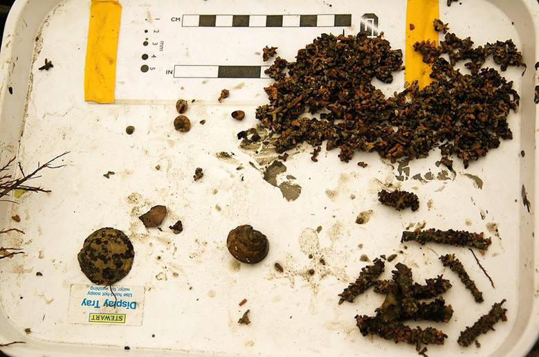
/Station%204%20brown%20and%20red%20algae%20with%20Undaria%20pinnatifida.jpg)
Station 4. Maerl Sample Station 4. Shell remains, Sabellaria tubes and maerl Station 4. The kelp Undaria pinnatifida and red algae
5. Bill Conway Estuary Sampling
Location and basic details
|
Date |
Lat. |
Long. |
Temp. |
Sal. |
Time |
Depth |
Tide |
Weather |
|
15/07/06 |
50’ 10.734 N |
005’ 03.166 W |
17.23 C |
34.84 psu |
0932 BST |
7.4 m |
HT = 1900 GMT LT = 1540 GMT |
1/8 cloud octants Wind ~ 4 m/s |
Introduction
The lower reaches and mouth of the Fal estuarine system represent a transition environment, a setting where characteristics and processes from both the inshore and offshore waters meet, creating a heterogeneous and ever changing environment. The Fal mouth is quite an open embayment of water, where swell and rough seas can migrate a few kilometers inside, generating at times a well-mixed environment. When transitional calm is reestablished at times, the system develops a thermally stratified structure and other parameters also correlate well with depth. A basic depth survey of this section of the estuary reveals a deep channel with adjacent shallower water, but still deep enough to bear a surface water layer, mixed layer, and a layer below the thermocline different from each other, as expected for the offshore environment. Nutrient concentrations will be at half way between the well-supplied lower and upper reaches waters, due to the input and anthropogenic sources at those sections, and may be limiting at times due to the dynamics of the system. Nutrient analysis can be combined with inshore data to monitor inorganic nutrients behavior from the very mouth of the estuary to a reasonable distance upstream. These kind of surveys are then of key importance to draw full pictures of the situation along the whole estuary system.
Phytoplankton and zooplankton may be expected represent both the inshore and offshore environments, with representatives found in previous surveys in such different atmospheres. Each particular functional group may have a downstream and upstream distribution and maximum reach, which could be modified by salt intrusions or freshwater flooding, as well as other factors. Temperature variations or whichever factor is modified, affecting the physiology of organisms can favor or avoid their migration in either way, leading to a difficult characterization of which are the limits for each species.
The physical structure also suffers from modifications and rapid variations depending of several factors. Freshwater intrusions from the riverine end member at flood times can modify to a great extent the dynamic stability of the system. Spring tides are also of great importance at this section of the estuary, given that the surrounding shores are fully impacted by the rising and ebbing tide. Swells, wind generated waves and other physical disturbances are well-felt at the mouth due to the open nature of the Fal, and the general picture of the water could be changed in a short time-scale.
Salinity changes on the horizontal are not great influenced, and variations of a factor of 2 or 3 can be regarded as normal from the mouth of the estuary to the end of the lower reaches. Temperature increases normally when heading towards the river source, but this is not to be expected at times of flood. It can be regarded as a typical situation for the summer period, when the low freshwater inputs, allow the water to stay warm (freshwater is colder than saltwater). The slow-moving surface waters at the upper and middle reaches may be well warmed by the increasing atmospheric temperature and by the time they reach the Fal, they are one or two degrees above the water there. The Fal environment is better mixed by physical processes, and then temperature can be a bit lower than the one coming from the riverine end member.
Materials and sampling procedure
The sampling effort as characterized by a time limitation that did not allow doing things as they were supposed to. Nonetheless, every effort was made to ensure a general picture of the estuary was taken, and processes going on, were well-characterized.
The material used was as follows:
- Bill Conway was used as the base boat, from
which all the deployments were carried out.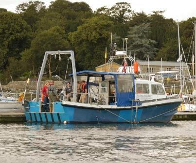
- CTD F7a was used on board, with GO-flow bottles, transmissometer and fluorometer.
- Two T-S probes were used. One measured salinity and temperature at all times, while the other was used to take direct measurements from the bottles on the chemistry table (three bottles per sampling station at three depths).
- A Secchi disk and a measuring tape were used to monitor the euphotic zone extension.
- A zooplankton net (200 microns) was deployed to sample the surface waters.
- A table with all the required chemical instrumentation, bottles, etc, was set up to process samples on board.
- A special programme onboard was used to analyze CTD results and process them for further analysis, as well as making decisions about where about to close sampling bottles within the water column.
- Other programme was used to analyze ADCP data, and transects were set across the estuary.
- An anemometer was used to record wind velocity.
- In order to lower the CTD gear into the water, a winch was used.
The sampling procedure aimed to cover a reasonable section of the estuary, from the very mouth, to the limit of the lower reaches, where the estuary narrows. The sampling strategy proceeded as follows:
- The previous day, a decision was taken, after considering the scarce time available, both for field work, and laboratory and data processing. A series of horizontal transects at 4 or 5 points were put forward, and a semi-continuous transect from the mouth of the estuary to the limit of the lower reaches was agreed to deploy CTD casts.
- ADCP was set up at these horizontal
transects, and up to 5 horizontal ones were taken at particular locations. The
first was towards the mouth, and the last one, where the estuary starts to
narrow. An additional transect was taken following a vertical line, contrary to
the previous horizontal ones, from The Narrows, further upstream.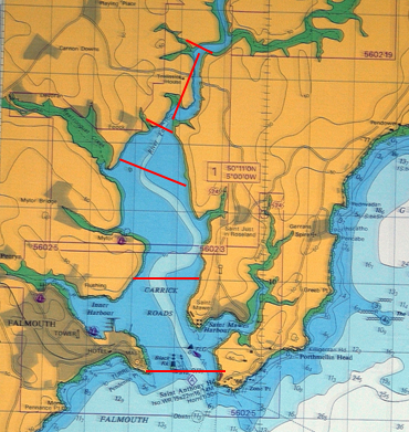 These are shown on the map in red.
- CTD casts were decided following the topography of the main deep channel, starting at the mouth (rough weather avoided the first casts), and heading upstream. The last cast was taken near The Narrows.
- CTD was lowered to a reasonable depth above the seabed, and after having a look to the vertical structure of the water column, a decision was taken about where about to close the sampling bottles. Particular attention was paid to the structure of the thermocline, trying to sample above and below it.
- Two zooplankton trawls were carried out, one at the mouth of the estuary (were sea conditions allowed), and another in the narrowed channel towards the end of the journey.
- Secchi disk deployments were carried out at each station.
- One person was specifically in charged of the meteorological data, which can be found as a stippled document on the logbook.
- Annotations on external forces/effects, affecting for example the ADCP readings were recorded at all times, in order to be able to analyze them successfully.
5.1 Bill Conway Estuary - Results
ADCP Analysis
Station 1
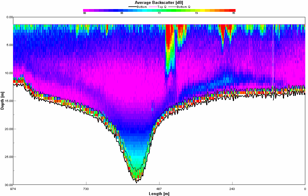
Average Backscatter
This site shows very little backscatter in the vertical water column, but in the surface waters there is a fair amount of sediment or zooplankton probably due to light availability causing phytoplankton to bloom. This hypothesis was analyzed later, and zooplankton abundance could be rejected because phytoplankton did not grow at the surface, but below 10 meters. Around 490 m length into the transect there is a big peak in the back scattering, this is a result of a large boat causing a wake and mixing up the water column.
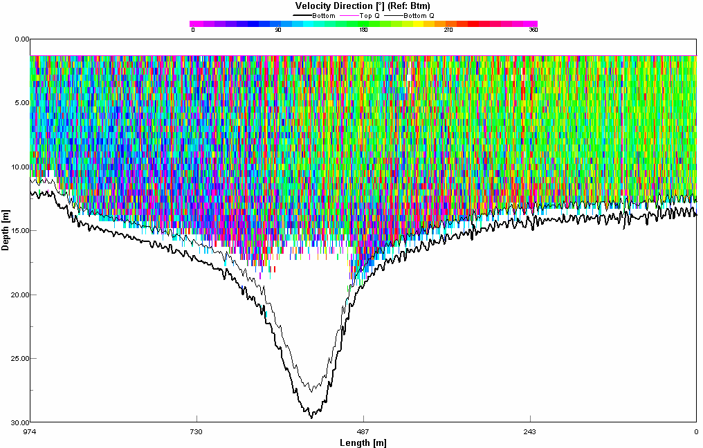
Velocity Direction
The direction of the flow is predominantly south easterly; the wind direction at this site was 120 degrees (southern), the tide was ebbing and fairly strong due to the fact that there had been a spring tide on the 14th July 2006 (i.e., the day before) which is the reason for the flow’s dominant direction, the velocity magnitude was only 0.125 – 0.250 m/s which is relatively low for a day which has a tidal range of up to 4.81 m. The reason for this is that the wind is from a southern direction which is opposing the tidal flow, the wind speed varied between 2-3 m/s which is not enough to affect the ebb tide being measured on that date. This is why there was a 2-3 m swell (which is caused by tides) and no significant wind driven waves.
Station 4
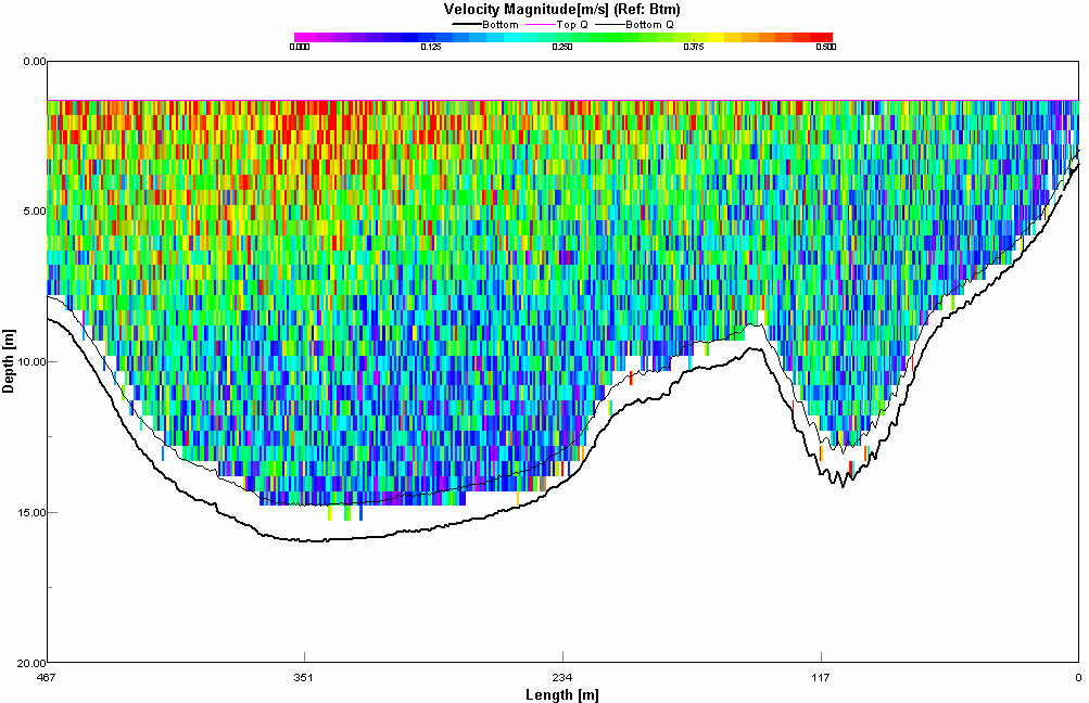
Velocity Magnitude
The velocity is much quicker in the surface waters at the end of the transect (closer towards the riverine input, which is due to the upper estuary getting narrower, which has a funnel effect forcing the water through quicker. As the water column gets deeper further downstream there is less pressure from the tide for the water to flow out as quickly, thus the velocity in the deeper waters is 0.125 m/s compared to 0.5 m/s at the surface.
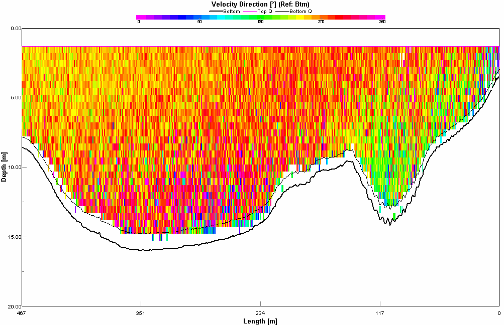
Velocity Direction
The direction of the flow is generally in a westerly direction this is probably due to the fact that we were are on a corner of a creek, as the wind speed was 0 m/s. As the transect came to an end at 407 m length, where the creek flows into the deeper channel of the upper estuary the velocity direction started to change to a more south westerly direction. This is because the tide begins to take effect and as the tide state is ebbing, it pulls the water south.
Station 6
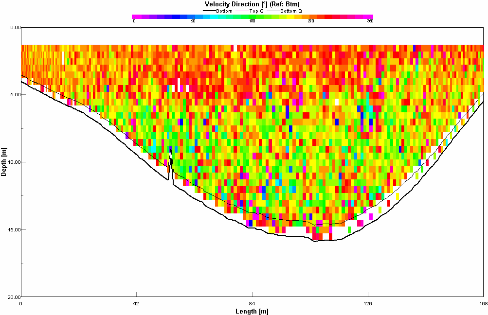
Velocity Direction
The velocity direction is westward at the surface but mostly southward below 5m, this is because the deeper water slows down and the tides take more of an effect; as seen in the velocity magnitude ADCP image. Where as in the surface waters the velocity magnitude is still large and momentum from the river flow pushes the surface waters, thus velocity is faster than in the deeper waters.
T-S Probe Data Analysis
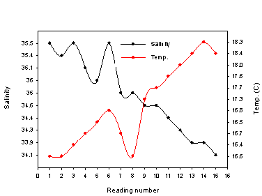 At
the same time ADCP and CTD casts were carried out, readings from a T-S probe
were performed at random times when drops in salinity and temperature were
observed. They were noted and analyzed as the survey went on, following a
logical progression transect from the mouth of the estuary to the Narrows.
Salinity changes were observed, but with a difference from 35.5 to 33.9, not
nutrient analysis could be taken with mixing diagrams. Nonetheless, this kind of
analysis has been done in the RIBs section. There was not much variability along
the estuarine area sampled (deviations from a straight line from the first
station to the last one). However, due to the lower than usual freshwater
inputs, the salinity readings at the last stations were still high.
At
the same time ADCP and CTD casts were carried out, readings from a T-S probe
were performed at random times when drops in salinity and temperature were
observed. They were noted and analyzed as the survey went on, following a
logical progression transect from the mouth of the estuary to the Narrows.
Salinity changes were observed, but with a difference from 35.5 to 33.9, not
nutrient analysis could be taken with mixing diagrams. Nonetheless, this kind of
analysis has been done in the RIBs section. There was not much variability along
the estuarine area sampled (deviations from a straight line from the first
station to the last one). However, due to the lower than usual freshwater
inputs, the salinity readings at the last stations were still high.
Temperature increased when heading towards the riverine end member, reaching almost two units difference between the first station and the last one. This temperature increase towards the river member may be a transient feature of the water masses. In winter times, the surface fresher waters may be colder than the seawater ones, and the temperature transgression will be the contrary as found during the summer times.
CTD Results and Discussion
Station 1
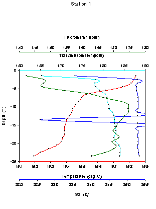
Taken at the mouth of the estuary, in waters 33 meters deep, the thermal structure was not well established, with a total change of 0.6 degrees from top surface to the bottom. The surface layers were a bit warmer, but not remarkably high, probably due to solar heating, and a well mixed water column, caused by its turnover due to water dynamics. Salinity structure revealed a less salty water layer on top of the water column, with a change of roughly a factor of two. This could be caused by increased river discharge due to recent inputs. The structure remained fairly homogeneous down to the seabed.
A chlorophyll peak was recorded at 10-11 meters, with low values in the surface layers, probably due to the rough sea state encountered, which could have interfered with positive algal development. A basic silicon analysis revealed depletion towards the deep layers, at the chlorophyll peak, and below it. It is presumed, diatoms could have caused it. Phosphate was found to be depleted just above the chlorophyll peak, while nitrate was removed constantly with depth. Turbidity increased positively with depth.
Station 3
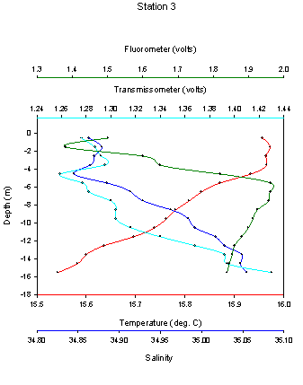
The slightly developed thermal structure at Station 1 has definitely been broken down at this point of the estuary, and an almost mixed water column developed. Indeed, only half a degree C change from the surface to the bottom occurs. Salinity also reflected a fairly homogeneous structure with depth. A chlorophyll peak developed at 5.5 meters depth. Compared with Station 1, depth was shallower at this station (18.8 meters), and consequently the chlorophyll peak was found in shallower water, reflecting the balance between nutrients from below and light inputs from above, a well as the dynamics of the system. Phosphate decreased with depth at this point, and nitrate was also reduced, after a slight increase at the surface, reflecting the probable absence of much algal growth at the very surface. Turbidity increased also with depth, as found at Station 1, with a slightly clear surface water layer.
Station 5
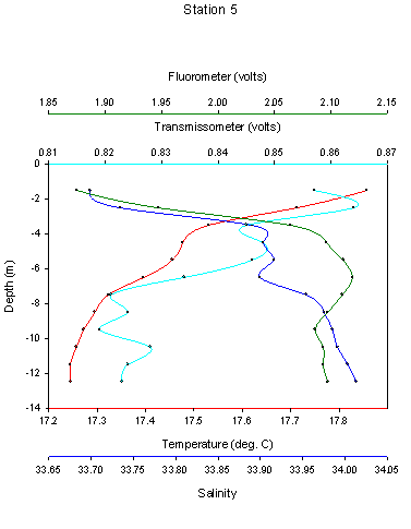
This station is found mid-way between the mouth of the estuary and the start of the Narrows. With a total depth of 19.2 meters, the thermocline was quite developed at this point, with a two degrees C drop in temperature. The surface water layers at this point were observed to be more stagnant that the ones towards the mouth, and it is supposed they have been warmed up over a longer period of time. The salinity structure did not show much variability with depth. Another chlorophyll peak was recorded between 6.5 and 7.5 meters depth. This was to be expected if bearing in mind the general picture described at the previous stations. Increased total depth, allowed for phytoplankton to be found a bit deeper than in the previous station. Turbidity also showed a peak, just below the chlorophyll one, probably indicating the mixed and favorable environment the alga may found at such depths. Silicon increased at 7 meters, which could be explained, as if no diatoms were present there, because nitrate concentrations decreased when going deeper, still supporting the present phytoplanktonic community.
Nutrient analysis (progression from the mouth to the freshwater end member)
Mixing diagrams were not used to asses the distribution of nutrients, because the sampled area did not show much salinity variations to compare, and a characterization of their behavior was not possible in this way. Nonetheless, mixing diagrams have already been used somewhere else (RIBs analysis), in order to draw a general picture of inorganic nutrients behavior.
Silica
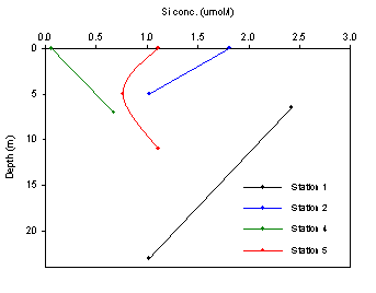
Progression from Station 1 to Station 5 reflected the sampling effort transect from the mouth of the estuary to the area past the Narrows. Therefore, bearing in mind this logical transect, nutrient behavior may change as plotted in vertical profiles, from Station 1 to Station 5. Silicon was not found to follow a logical progression, increasing in concentration when heading to the freshwater end member. Station 1 and Station 2 were found to have the highest concentrations, which was not to be expected, as these stations were the further offshore. It cold reflect however, diatom growth along this transect of the estuary, with some slow moving, well stratified waters. The well-mixed water at the mouth may not allow successful diatom development and their optimum growth is reached further upstream, where the water vertical structure meets the algae necessities.
Phosphate
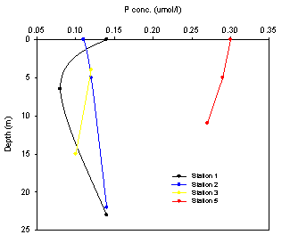
Phosphate followed a roughly logical distribution when heading towards the freshwater end member. The progression from Station 1 to Station 5 was reflected as an overall increase in the phosphate concentration. Particularly remarkable was this nutrient profile at Station 5, were it remained much higher than at the other locations. This situation could be explained as a presumably enrichment in phosphate from the freshwater inputs, which was found in the RIBs analysis. The catchment of the Fal is well supplied from agricultural runoff as well as other sources, which show up as increased concentrations for both phosphate and nitrate.
Nitrate
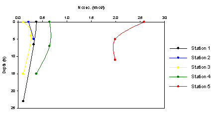
Nitrate behavior was quite parallel to phosphate, in the sense that there was a reasonable progression from the saltwater masses to freshwater end member. Station 1, 2, and 3 were remarkably depleted (not completely) on this nutrient, probably indicating the algal activity at those areas. Station 4, and particularly Station 5, was well supplied with this nutrient, presumably indicating, as in the case of phosphate, enrichment from the different sources described in the RIBs section
Plankton Analysis
Phytoplankton
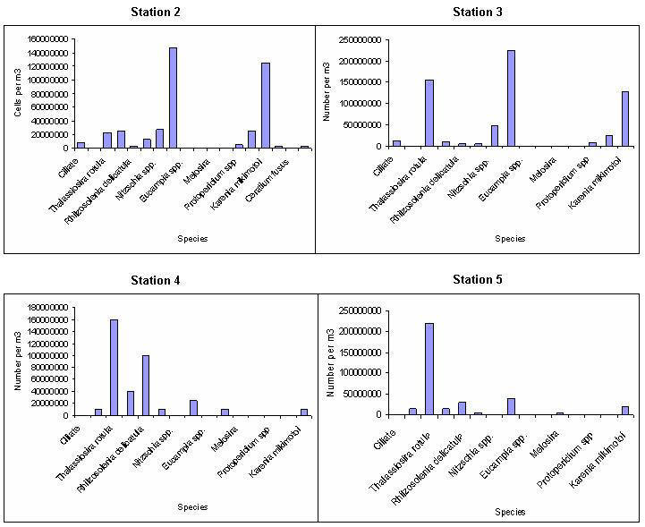
Diatoms are the dominant group of phytoplankton t all of the stations. They are particularly dominant at the second station where the concentration of silica is highest. There are slightly higher numbers of flagellates at station 5, in the river although the high salinities indicate that there is little river flushing and this has lead to a small concentration in silica keeping a population of diatoms alive. Phosphate and nitrate concentration are also highest at station 5 which appear to cause a bloom in Thilassiosira rotula in this region.
Zooplankton
Station 1
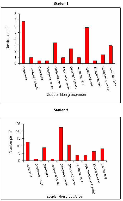
At station 1, situated at the mouth of the Fal estuary, a zooplankton sample was obtained from a 2 minute zooplankton net tow. The results showed very low numbers of zooplankton in the water. The dominant species were Copepoda and Hydromedusae, with approximately 2 every litre of water. All other species showed lower concentrations than this indicating very low biodiversity in the area. This is likely to be caused by low concentrations of phytoplankton in the area limiting the zooplankton growth by lack of food, as well as other unknown factors. The well-mixed water column in the area also means that the zooplankton may find it difficult to stay in the surface layer where the phytoplankton would be most active, or they may be mixed and moved in different ways depending on the water dynamics and species-species capabilities.
At station 5, however, which was much further up the estuary near the head, the zooplankton was present in much higher concentrations. In this area Cirrepedia larvae dominate with Copepoda and Gastropod larvae also present in high amounts. This could be accounted for by increased amounts of phytoplankton in the water, as a less turbulent, more sheltered area of water may create a more stable environment allowing phytoplankton to flourish. This in turn allows zooplankton to flourish as they are not limited by food availability.
References
Bryan, G.W. and Langston, W.J. 1992. Bioavailability, accumulation and effects of heavy metals in sediments with special reference to UK estuaries: a review. Environmental Pollution, 76, 89.131.
Cameron, W. M. and D. W. Pritchard. 1963. Estuaries. In M. N. Hill (editor): The Sea vol. 2, John Wiley and Sons, New York, 306 - 324.
Evans, C.D.R., 1990. United Kingdom Offshore Regional Report: The Geology of the Western English Channel and its Western Approaches. HMSO for the Brit. Geol. Surv. London, 93 p.
Hosking, K.F.G. and Obial, R. 1966. A preliminary study of the distribution of certain metals of economic interest in the sediments and waters of the Carrick Roads (West Cornwall) and of its “feeder” rivers. Canborne School of Mines Magazine, 17.36.
Kiorboe, T. 1993. Turbulence, phytoplankton cell size, and the structure of pelagic food webs. Adv. Mar. Biol. 29: l-72.
Langston, W.J., Chesman, B.S., Burt, G.R., Hawkins, S.J., Readman, J. and Worsfold, P. 2003. Site characterisation of the South West European Marine Sites. Fal and Heldford cSAC. Marine Biological Association, Citadel Hill, Plymouth, PL1 2PB.
L-3 Communications SeaBeam Instruments. Sidescan. 2000. Multibeam Sonar Theory of Operation.
Parr, W., Wheeler, M. and Codling, I. 1999. Nutrient status of the Glaslyn/Dwyryd Mawddach and Dyfi estuaries; its context and ecological importance. WRc Final Report to the Countryside Council of Wales.
The views and opinions expressed on this website are those of the individual and not necessarily thoses of Southampton University
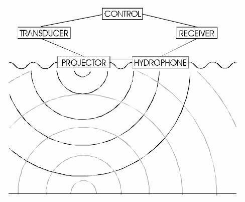
/Geophysics%20map%20track.JPG)
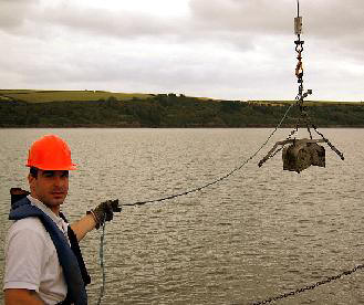
/Bottom%20sampling%20map.JPG)