Falmouth Field Course - July 2006
- Group 1 -
![]()

Emily Boram, Alessandra Curiel, Thomas Harper, Alexander Payne, Katherine Read,
Katie Saverymuttu, Robert Smith and Clare Usherwood
| Offshore - Callista |
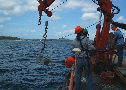
04/07/06 Weather: Anticyclone over the last couple of days, foggy with a visibility of approximately 300m, light breeze, 8/8 cloud cover. Time of Departure: 11:20 GMT Equipment: CTD, Niskin Bottles, Plankton Net, ADCP, Light Profiler, Secchi Disk PSO: Katie Read |
|
07/07/06 Weather: Breezy, warm, calm water. Cloud cover 5/8 Time of Departure: 09:00 GMT Equipment: Niskin Bottle, Plankton Net, Secchi Disk, Plastic bottle for sampling surface waters PSO: Clare Usherwood |
|
| Estuary - Bill Conway |
14/07/06 Weather: Sunny, warm, breezy. Cloud cover 0/8 Time of Departure: 08:39 GMT Equipment: CTD with rosette of Niskin Bottles, Plankton Net, Secchi Disk, TS Probe, Weather Station PSO: Tom Harper |
| Geophysics - Grey Bear |
11/07/06 Weather: Cloudy with sunny spells, 4/8 cloud cover Time of Departure: 09:35 GMT Equipment: Towed Side Scan Sonar, Stacked Sieve, Display Tray PSO: Rob Smith |
|
|
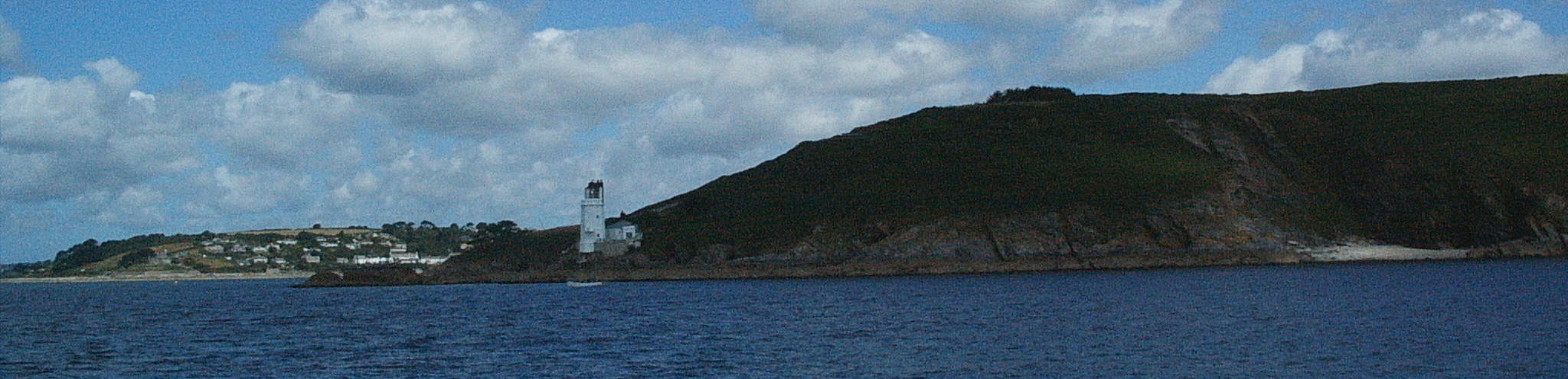
Introduction to the Falmouth Estuary
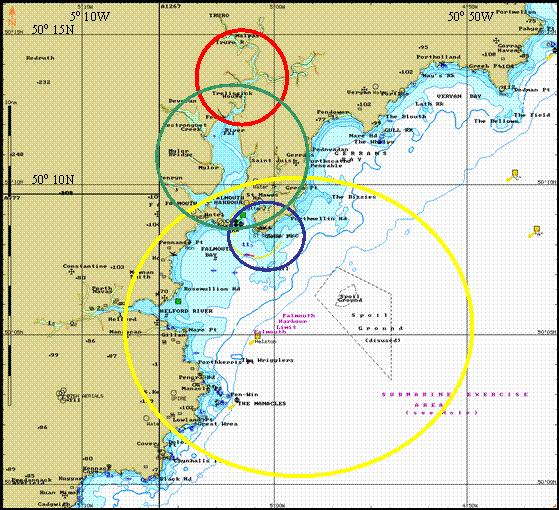
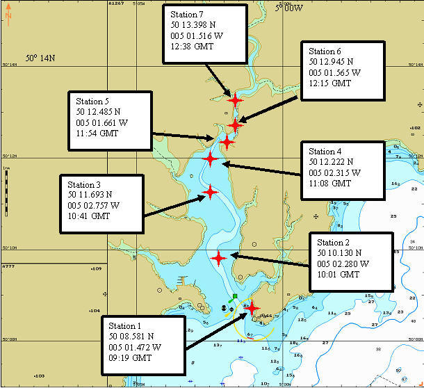
Fig 1. Overview map of locations sampled Falmouth Estuary is located on the southern Cornish coast and forms the large and sheltered natural harbor of Carrick Roads, a drowned valley at the junction of seven rivers. The Fal Estuary is a drowned river or 'ria'. The deep water channel which winds its way upstream to Truro dates back to the last Ice Age when the sea level was much lower than at present. It is the third largest natural harbor in the world and the area known as Carrick Roads extends four miles from Black Rock to Turnaware Point with nowhere being less than one mile wide. Falmouth, the principal Port of Cornwall, lies at the mouth of the Fal Estuary on the South West coast. The Fal estuarine system is characterized by a mean spring tidal range of 5m and tidal currents reaching 2 knots. Prevailing winds come from the South-west, mean surface water temperatures in summer are approximately 16°C and salinities in the open coastal waters surrounding the Fal are in the region of 35. Extensive sea grass (Zostera) beds and the Coralline algae (Maerl) beds exist in the Fal estuary and have contributed to the classification of the estuary as a Special Area of Conservation. The Fal region has been subjected to a history of pollution events due to heavy mining activity in the estuaries catchment area, along with domestic sewage effluent discharge. Localized effluent input continues in Carnon Valley, along with input from the County Adit, and there was a notable discharge of mining effluent (containing high heavy metal concentrations) into Restonguet Creek during the 1990’s. This has lead to increased metal levels detected within organisms in the Fal and some genetic adaptation of organisms to survive in the more polluted locations. The combination of metal pollution and increased nutrient inputs has also led to the occurrence of red tide events (post 1995) due to blooms of the dinoflagellate Alexandrium minutum, resulting in paralytic Shellfish poisoning. |
|||||||||||||||||||||||||||||||||||||
R/V Callista
Fig 16
Fig 17
Fig 20
Fig 24
Fig 26 |
|
Fig 2. Map showing offshore sample locations
Fig 4. Backscatter at Carrick Roads
Fig 5. Velocity Magnitutde for Carrick Roads
Figure 7. The velocity magnitude at the offshore station
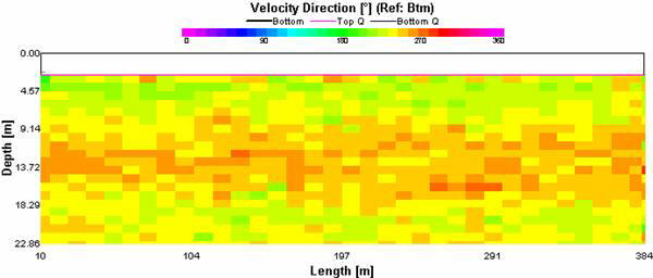
Figure 8. The velocity direction at the offshore station
Figure 10. The velocity magnitude at St Anthony Head 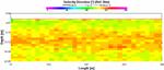 Figure 11. The velocity direction at St Anthony Head
Fig 12
Fig 13
Fig 14
Fig 15
Fig 18
Fig 19
Fig 21
Fig 22
Fig 23
Fig 25
|
||||||||||||||||||||||||||||||||||||
|
R/V GreyBear
Fig 31
Fig 34
Fig 35
Fig 36
|
Geophysics - R/V Grey Bear Aim: The aim of the boat work was to develop an understanding of the underwater area East of Falmouth Estuary taking into consideration the bedforms, rock type, sediment type and marine species present at the sites. Objectives: To meet this aim we used the following objectives:
Key Outcomes: Planning: As the area East of Falmouth Estuary had not previously been studied it was decided to carry out 5 transects measuring 2km in length. The sidescan sonar results will then be used to determine appropriate locations for the van veen grab. Stations that are presumed to be appropriate are those that display characteristics of soft sediment and not rock substrata. The strategy can therefore, be adapted depending upon the sidescan sonar results. Locations:
Equipment:
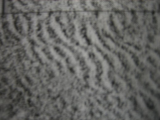
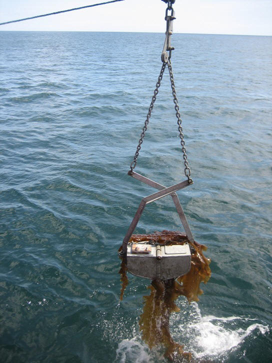
Sampling: In order to understand the geology of the area the sidescan sonar was towed as a fish 1m below the surface of the water and 1m behind the stern of the Grey Bear. The fish was towed at 3knots along 5 transects. A paper print out of the sidescan sonar was produced, as the transects were carried out, and analysed for potential grab sites, i.e. those with a finer sediment type. Once appropriate sites were identified a Van Veen grab was deployed and observations were made upon the material brought back up.
Once back in the lab the sidescan sonar was further analysed to determine the sediment type, the size of the ripples present in the sediment and the direction of the strike of the rock. A map was then produced of the features observed. Complications: There was difficulty in selecting the grab sites as the majority of the area surveyed was rock. Results: Bedform Ripples Off St. Anthony Head The ripples illustrated at 50°083N 005°00.7W were on the sidescan sonar plots are a result of shallow water waves. The waves are defined by:
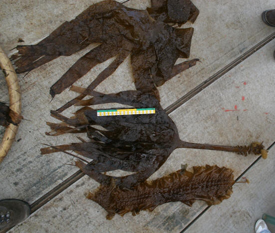
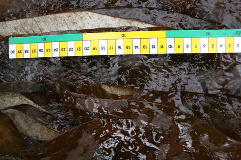
d < λ / 20 where d: depth λ: wavelength It can be shown that the wavelength of the waves which caused the ripples were of a wavelength great enough to cause an influence on the sea bed. Such bedforms are characteristic of storm waves. For these bedforms to remain unscathed, the tidal influence in the area must have little effect on the seabed. Admiralty charts illustrated that the tidal waves in the area of these bedforms propagate perpendicular to the coast line, hence currents are unable to remain for long enough to reshape the seabed. Site 1 Position: 30330N, 184754E Time: 12:10:43 AST Water depth: 14m The plan was to sample on soft sediment identified as an area of uniform backscatter from the side scan record. However the sampling position may have differed from the expected position causing us to sample on bedrock. Sediment: No sediment collected at site due to sampling on solid bedrock. Biology: Collected Kelp from bedrock in an area of possible extensive kelp forests. Site 2 Position: 30449N, 184638E Time: 12:21:08 AST Water depth: 10m Again the plan was to sample on an area of uniform backscatter identified as soft sediment. This was at the boundary between rock and weed (R.Wd) and stone with broken shells (St.bkSh) as shown on nautical chart of Falmouth harbour (5602.5). Again the desired sample wasn’t attained and the sample was believed to have been taken on solid bedrock. Sediment: no sediment collected due to sampling on solid bedrock. Biology:
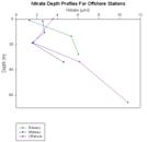
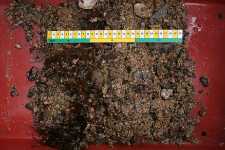
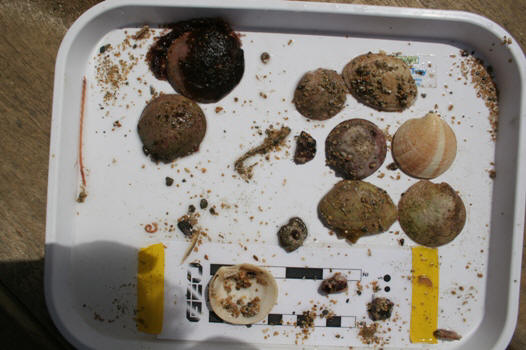
Site 3 Position: 30635 N, 184648W Time: 12:48:48 AST Water depth: 13m The expected sediment sample was stone with broken shells (St.bkSh) as identified by previous sediment grabs in the location noted on nautical charts of the area. The area sampled was shown as a uniform area of backscatter, initially interpreted as an area of soft sediment. Sediment: 20% of the sediment sample was <500µm and 75% was >1mm. The remaining sediment consisted of stone and broken shells as expected. Biology:
Lepidochtuna cinereus Peppery Furrow Shell (Sciobicularia plana) Limpet
Site 4 Position: 30629N, 185005E Time: 13:28:19 AST Water depth: 12.8m The plan was to sample on sediment identified in the side scan record as uniform backscatter. However sampling again collected only kelp and it was believed sampling had taken place on solid bedrock. Sediment: No sediment collected at site due to sampling on solid bedrock. Biology: Collected Kelp from bedrock in an area of possible extensive kelp forests. Also identified was Palmaria Palmata which is a type of seaweed. Site 5 Position: 30455N, 185138E Time: 13:40:40 AST Water depth: 10m The plan was to sample again on sediment identified in the side scan record through an area of uniform backscatter. However sampling took place on rock and weed as before. Sediment: No sediment collected at site due to sampling on solid bedrock. Biology:
Conclusion: Our geophysics survey showed that most of the seabed we surveyed was found to be hard rock, with some smaller areas of softer sediments found in between the areas of bedrock. The softer sediments, which showed bedforms and ripples tended to be found closer to the shoreline. Our grabs showed that areas which we originally thought were softer sediments were often kelp forests. These were shown by homogenous areas of backscatter on the side-scan record. Four out of five of our grabs showed areas of hard rock with maerl and kelp thriving. Our other grab showed an area of softer sediment found closer to the shore. This grab showed a high diversity of benthic species surviving in cohesive sediment, consisting of stone and bioclastics, along with a finer grain sand. |
Fig 27
Fig 28
Fig 29
Fig 30
Fig 32
Fig 33 | ||||||||||||||||||||||||||||||||||||
|
Ocean Adventure
Coastal Research |
Estuary - RIBs Weather: 5/8 cloud cover, slight SW breeze, calm water. Tides: (GMT) 0800 1.94 1400 4.38 2030 1.96 Aim: To investigate the salinity change in the upper reaches of the estuary, with turbidity, dissolved oxygen content, plankton numbers, nutrient concentration and chlorophyll concentration as investigative factors. Objectives: The following objectives were used to accomplish our aim:
Planning: The upper reaches of the estuary were assumed to be typical of the fresh/salt water mixing interface with salinity near 0 being attainable at the top of the estuary. Sampling at set salinity intervals was a practical plan as it accounts for differences in chemical concentration at all stages in the river, (as the mixing interface may be over a short distance which geographical sampling could miss out). After initial sampling it was realised that this mixing interface was in the very upper reaches of the estuary, (a flooding tide and lack of freshwater input were attributing factors) so geographical sampling sites were set downstream of Truro instead to test for any changes in the investigative factors at a more or less constant salinity ~ 30. Locations:
Equipment: Two shallow water vessels, a Rib and a Dory, each having a YSI probe for salinity, depth and light attenuation data collection. Each vessel was equipped with a Secchi disk and a Niskin bottle, and equipment for holding different chemical samples. This included glass bottles for nitrate, phosphate and oxygen sampling, plastic bottles for silicate sampling and test tubes for storage of the glass fibre filters which were used for analysis of chlorophyll concentration. A plankton net was carried on board the Dory for 2 trawls at desired points along the estuary. Key Outcomes:
Sampling: At each geographical station a depth profile was taken with the YSI probe measuring Salinity, Temperature, Dissolved Organic Matter and pH a 0.5m intervals. A Secchi Disk was used to find the light attenuation depth at each station. At the stern of the vessels, chemical samples were taken by collecting a large amount of water from the surface and passing 50ml through a glass microfibre filter for both nutrients, (phosphate and nitrate sample) and silicate. The samples were refrigerated and the microfibre filters were stored in test tubes for chlorophyll analysis back at the laboratory. Dissolved oxygen content was measured only once on each vessel, (equipment allowing) at stations A and B3. These were collected under the surface layer by taking a horizontal sample with the Niskin Bottle. Once prepared, they were stored submerged in a container of sea water. Aboard the Dory two plankton trawls were deployed at Stations A and B which were preserved with formalin for analysis back at the laboratory. Complications: The original plan was to sample at salinity intervals from the sea, going up the river with increasing freshness. However, on the day of sampling, the tides meant that the sea water followed us up the river and so salinity wasn’t decreasing. The plan then changed to sample at geographical locations down the river. The stations are placed in the following order down the river: B2, B3, B4, B, B5, B6, C, B1, B7, A, D. Station B1 and B2 were sampled before we changed plan, and hence before the tide got up the river. This explains the lower salinities recorded for these two stations, and also why the salinities don’t necessarily increase as you progress down the river to the sea. Results: Zooplankton Figure 28 displays the % of total abundance of which zooplankton identified in the taxonomic identification, contribute to the total zooplankton abundance at each sampling station. The most abundant zooplankton species were Copepoda, which contributed ~58% of total zooplankton abundance at both stations A and B. The water sample from station A also contained 27% Cirripedia larvae, with station B containing 18% of the same zooplankton species. Station B also contained ~10% Gastropod larvae, with station A containing ~3% of the same species. Hydromedusae were also present at both stations, as were Copepoda nauplii. Both species contributed ~5% to total zooplankton abundance at station B and <2% at station A. Additionally Polychaeta larvae and Bryozoa were identified at station A, contributing <1% to total zooplankton abundance in both cases.
Phytoplankton From the total % abundance graphs for phytoplankton (Fig. 39) it can be seen that station C has the highest amount of Rhizosolenia with about 64%, compared to station A and B of which had percentages of 13 and 34. The dominant species found at station A was Thalasiocira which contributed 46% to the total abundance. This species was not found at any other site. Guinardia floccida was found at station A in small amounts (1%) and station C with about 5%. One of the few species found at all 3 sites was Chaetoceros sp stations B and C had relatively low amounts, only 10% whereas station A had a large proportion of its abundance made up by this species (34%). Nitzchia had low was in very low abundance up the river it was only found at station A and B and it was >1%. Ceratrium was only found at station B and in very small amounts. The main contribution to station B was N.Longissima making up 51% of the total abundance; it was also found in the water column at station C but in much smaller quantities. The species Rarenia mikimotoi and Mesodinium rubrum were both found at station A but in small amounts >2%. At station B Eucampia sp and Thalasiovia made up very small % abundance. It was found that at station C Coscinodiscus contributed 12% to the abundance and the final few percentages were Eucampia sp and Thalassiosira. Figure 40- graph comparing phytoplankton and zooplankton numbers. At station A phytoplankton and zooplankton numbers were lower than at station B, station A had a phytoplankton number of 127900 cells/l whereas station B had a phytoplankton number of 626000 cells/l. Phytoplankton might be limiting the population and numbers of zooplankton because phytoplankton are zooplankton’s primary food source. At station B the larger phytoplankton population is able to support a larger zooplankton population. Salinity Profiles Figure 41- Salinity profile for upper estuary. The profile shows salinities increasing with depth at all stations. The fresher riverine input from the Fal is less dense and hence sits above the more saline water. The salinities are typically lower at stations further up the estuary due to increased freshwater input and decreased mixing. It is well mixed at depth, indicated by the consistent salinity, despite varied surface salinities.
Figure 42- Salinity profile for the lower estuary The profile shows increasing salinities with depth at all stations. There is a fresher layer overlying a denser saline layer. The salinities for this profile are higher than those of the upper estuary, as the fresh water input of the Fal is less pronounced, and increased mixing with seawater increases salinity. Station B6 shows a text book surface fresh layer with a peak in freshness at approx. one meter.
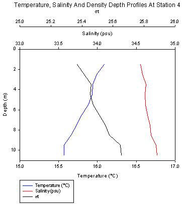
Figure 43- Temperature profile for the upper estuary The profile shows temperature decreases with depth. Surface temperatures are elevated by increased solar radiation and reduced wind stress which leads to the formation of a seasonal thermocline in the summer months.
Figure 44- Temperature profile for the lower estuary The profile shows temperature generally decreases with depth. This is due to the decreasing solar radiation. Station B6, concurrent with the surface fresh layer (shown in figure 2), shows a surface layer temperature peak. The lower estuary appears to fairly less well mixed at depth than the upper. Oxygen and pH NB: Two RIBS were used to collect the data. Ocean Adventure sampled station B1, B2, B3, B4, B5, B6 and B7. Coastal Research sampled stations A, B, C and D. The probes were not calibrated. Groups that sampled before us in the week experienced varied data between the probes used on the different boats, and carried out calibration work in the lab to check the reliability of the probes and hence the data. The results show that the probes were too different and hence the data cannot be quantitatively trusted. The trends however can be observed and should give a fair representation of what was going on. Figure 45- Dissolved oxygen profile for the upper estuary The profile shows in general oxygen decreases with depth. This could illustrate a phytoplankton layer with net respiration shown by the oxygen decrease. The water column appears well mixed at depth, with a fairly consistent oxygen level. With the elevated riverine input, turbidity levels would be useful as sediment input would limit light penetration, and hence it cannot be assumed that the shallowness of the water assures light penetration to depths for biological activity.
Figure 46- Dissolved oxygen profile for the lower estuary The profile shows oxygen levels decreasing with depth, possibly due to phytoplankton activity, although nutrient levels will be needed to collaborate this.
Figure 47- pH profile for the upper estuary The profile shows pH is fairly consistent with depth in the upper estuary. Station B shows an increase with depth.
Figure 48- pH profile for the lower estuary The profile shows pH is fairly consistent with depth in the lower estuary Richardson number = 0.696 This means the water mass is relatively stable, however it has come from an unstable source. Secchi Disk The depth of the euphotic zone generally increases as you move out to sea. The sediment in the river will decrease the euphotic depth, as the increased turbidity absorbs and scatters the light, thus decreasing the depth to which it penetrates. Stratification at the lower end of the estuary will aid light penetration to depth, as illustrated by the deeper euphotic zones.
Conclusion: Estuarine mixing diagrams from the estuary for nitrate, phosphate and silicate indicate that the nutrients are behaving conservatively with regards to salinity. There is no indication that addition or removal is occurring, however as nutrient samples were only collected at a limited range of salinities this is not conclusive. Nutrient concentrations display a gradient from the lower estuary toward the head with increasing concentrations moving up stream. Elevated nutrient concentrations in the upper estuary are supporting a large plankton population. This consists of both a phytoplankton and zooplankton population with the zooplankton grazing the phytoplankton. The gradient of nutrients identified through water column samples is also evident through the distribution of phytoplankton through the estuary, with the large phytoplankton populations coinciding with high nutrient concentrations. Temperature and salinity profiles in the estuary indicate a typical partially mixed estuary type (2 on the Hansen-rattary classification diagram) exists in the estuary with a deepening thermocline moving toward the estuary mouth. Stable stratification appears to exist at all of the station but of varying degrees of stability. Profiles of the estuarine pH indicate increasing alkalinity moving toward the estuary mouth, although the difference in the pH between the lowest station and the station closest to the estuary head is minimal (<1 pH). Due to sampling taking place as salinity moved up the estuary this brief study may be far from the true picture. Future work should concentrate on mapping nutrient distributions over many salinities and covering multiple tidal conditions to provide a more accurate view of the Fal estuary.
|
Fig 37. Map showing stations sampled in the estuary by the RIBs
Fig 38. Zooplankton Abundance
Fig 39. Phytoplankton abundance
Fig 40
Fig 41
Fig 42
Fig 43
Fig 44
Fig 45
Fig 46
Fig 47
Fig 48
| ||||||||||||||||||||||||||||||||||||
|
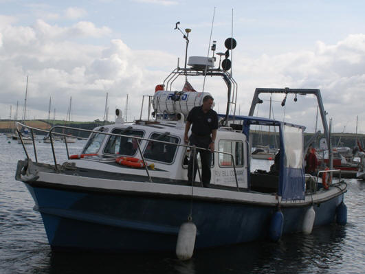
R/V Bill Conway
Fig 55
Fig 56
Fig 57
Fig 58
Fig 65
Fig 66
Fig 67
Fig 68
Fig 69 |
 Estuary - R/V Bill Conway Weather: sunny, 0/8 cloud cover, breezy Tides: (GMT) 0720 5.19m 1350 0.71m 1940 5.54m Aim: To assess the extent of vertical mixing processes in the estuarine waters off Falmouth and to collect information on nutrient concentrations and plankton numbers in said areas. Objectives: To meet this aim we used the following objectives:
Key Findings:
Planning: In order to achieve a comprehensive understanding of the estuarine system in Falmouth Harbour the following plan was devised. Transects will be carried out across the river at various points. These transects will look at the currents present in each location. Further studies on the physical, chemical and biological structure will be carried out using a CTD will niskin bottles attached. Locations: See map -> Equipment:
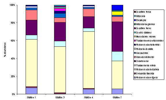
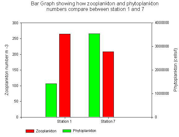
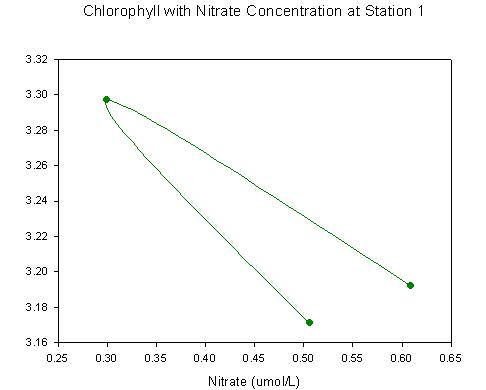
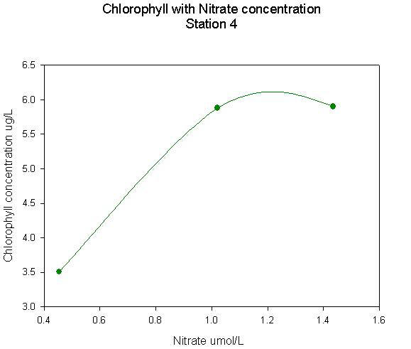
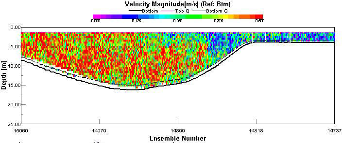
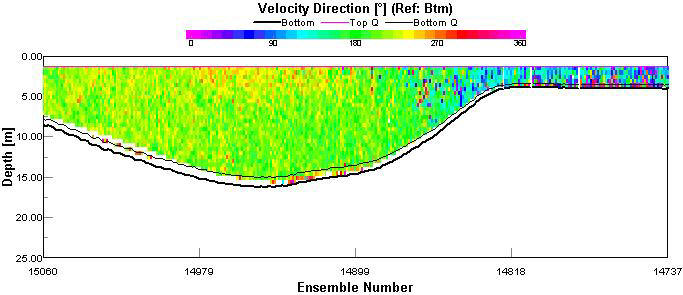
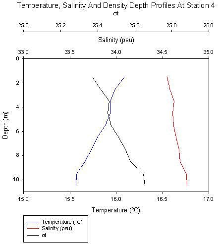
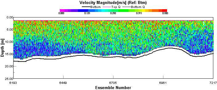
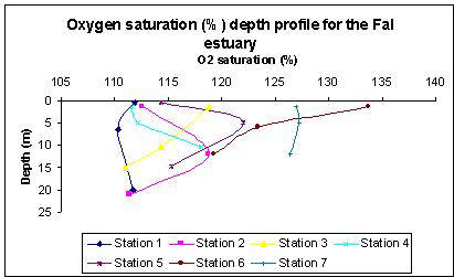
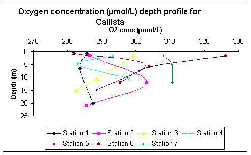
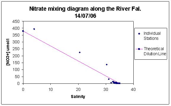
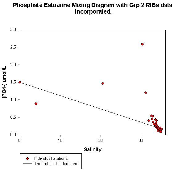
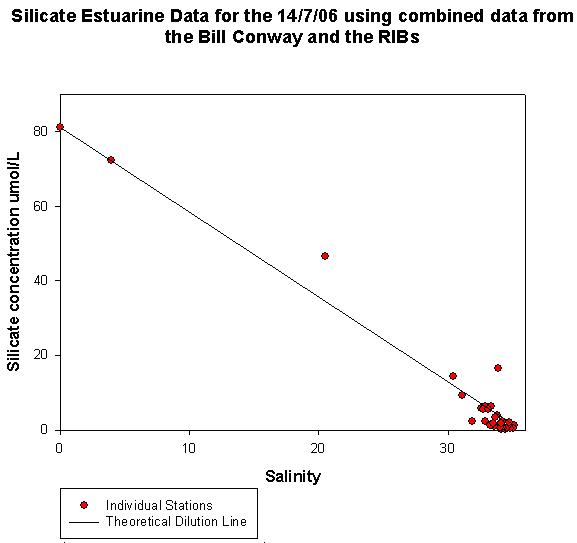
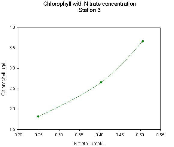
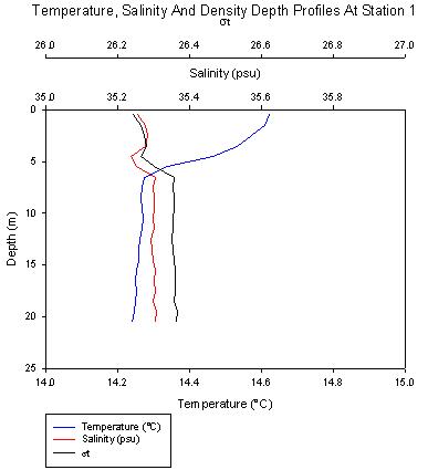
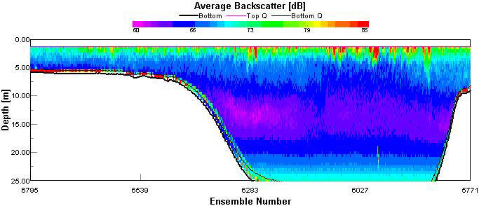
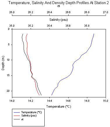
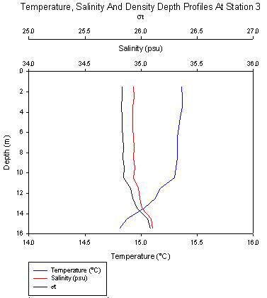
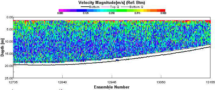
Sampling: At each sampling station a depth profile was taken with the CTD probe measuring Salinity and Temperature A Secchi Disk was used to find the light attenuation depth at each station. Chemical samples were taken by collecting a water from desired depths, (decided by analysing the CTD and ADCP outputs after a single deployment). and 50ml of sample water was passed through a glass microfibre filter for both nutrients, (phosphate and nitrate sample) and silicate. The samples were refrigerated and the microfibre filters were stored in test tubes for chlorophyll analysis back at the laboratory. Dissolved oxygen content was measured at each station using sample waters from each depth. Once prepared, they were stored submerged in a container of sea water. Zooplankton trawls is carried out at the sea-end member and the estuarine end-member for 2 minutes at 1.5 knots. At station 6 the equipment, including temperature probe and salinity probe was calibrated with that of the ribs. Complications: There are no known complications when collecting data for this investigation. Results: Chemical The oxygen saturation within the estuary varies strongly between stations (Fig.50) with a gradient from lower saturation at the estuary mouth (~112% saturation) to higher oxygen saturations moving upstream (127-134% at the stations closest to the estuary head). There is a sharp fall in oxygen stations moving downstream from station 6 (~134%) to station 5 (~114%) with the stations lying upstream and downstream of a mussel farm located in the estuary channel. The oxygen concentrations (Fig.51) reveal a similar picture with a gradient from low oxygen concentration at the estuary mouth (~285 µmol l-1) to higher oxygen concentrations at the upper stations (~326 µmol l-1). There is again a sharp change in oxygen concentrations between stations 5 and 6 with a change of 44 µmol l-1 between the stations. The estuarine mixing diagram for nitrate (Fig.52) indicates addition of the nutrient is taking place in the estuary between a salinity range of 5-30. At higher salinities it appears that the nutrient is then behaving conservatively. Addition of phosphate also appears to be taking place (Fig.53) within the estuary, whereas silicate (Fig.54) is behaving conservatively with regards to salinity. Biological Analysis Zooplankton Figure 55 displays the % of total abundance of which zooplankton identified in the taxonomic identification, contribute to the total zooplankton abundance at each sampling station. The most abundant zooplankton species were Copepoda, which contributed ~42% of total zooplankton abundance at station 1 and 61% at 2. The water sample from station 7 also contained 32% Cirripedia larvae, with station 1 containing 18% of the same zooplankton species. Station 1 also contained ~12% Gastropod larvae, whilst station 7 contained none of the same species. Hydromedusae were also present at both stations, as were Cladocera. Additionally Appendicularia larvae were identified at station 1, contributing ~8% to total zooplankton abundance. Phytoplankton From the total % abundance graphs for phytoplankton (Fig. 56) it can be seen that for all stations the most abundant phytoplankton is Rhizosolenia delicatula. This phytoplankton is most abundant at station 4 where it contributes to 64% of the station’s phytoplankton. At stations 1 and 3 Rhizosolenia delicatula contribute ~50% of total abundance and at station 7 they contribute the least to total abundance at ~31%. The dominant species found at station 7 is Chaetoceros which contributed ~33% to the total abundance. This species was found at the other sites but at slightly lower % of total abundance ~15%. Rhizosolenia setigera was found at stations 1,4 and 7 contributing ~6% to total abundance. This species was found in negligible amounts at station 3. The species Karenia mikimotoi was found at all 4 stations, contributing ~11% at station 1, ~5% at station 3, ~9% at station 5 and ~6% at station 7. Thalassiosira rotula was also found at all four stations contributing the largest percentage of ~11% at station 7 and ~5% at the other 3 stations. The species Eucampia was only found at station 7, representing 6% of the total abundance. This may be because this species favours slightly fresher lower salinities. At station 7 higher phytoplankton levels are seen compared with station 1. At station 7 there are 3540000 phytoplankton cells/L, which is over double the number seen at station 1 where there are 1420000 phytoplankton cells/L. Lower zooplankton levels are seen at station 7 compared with station 1. At station 1, 265 m-3 compared with 209m-3 at station 7. The elevated zooplankton levels seen at station 1 accompanied by the lower phytoplankton levels could be due to the large zooplankton population cropping the phytoplankton population. The area around station 1 at the time of sampling could be in the later stages of a bloom, where phytoplankton numbers are now decreasing and zooplankton numbers are still large due to the lag behind the phytoplankton decline after the bloom. At station 7 a slightly smaller zooplankton population exists accompanied by larger amounts of phytoplankton. Station 1 (Fig 57) indicates that higher nitrate concentrations are present in deeper water but that the phytoplankton population is only present in the upper (surface) layer. This shallow phytoplankton population corresponds to the shallow secchi disk observation, and is possibly as a result of high turbidity in these waters (during the data collection sea conditions were stormy, resulting in a well mixed water column). Fig 58 and Fig 59 demonstrate a positive relationship between nitrate and chlorophyll, indicating higher chlorophyll concentrations coincide with high nutrient concentrations. Physical: The ADCP and the CTD were two instruments used for physical data collection aboard the Bill Conway. These instruments allowed the analysis of the estuarine dynamics with respect to water salinity, temperature, density, flow velocity magnitude and direction. There is a noticeable trend up the estuary of flow direction and velocity associated with the temperature and salinity of the water. At the mouth of the estuary, the water column was generally well mixed with uniform velocity magnitude and direction. A seasonal thermocline was present at station 1, as seen in Figure 60. The Richardson number for this location at the thermocline was 0.17. Hence, the water column is mixed however not enough to cause the breakdown of the thermocline. The mean water velocity was 0.125m/s. Backscatter between 10m and 15m decreased to 60dB, indicating the presence of a thermocline and a dominant zooplankton population. As the vessel progressed up the estuary, the presence of fresh water became more dominant, a non uniform flow becomes increasingly influential. The non uniform flow below 15m water depth was overlaid by a well mixed water with a velocity ranging between 0.125m/s - 0.250m/s. Station 2 had a higher velocity of 0.5m/s on the water surface, the water column mean water velocity was 0.250m/s. The Richardson number was calculated as 0.02, indicating the dominance of shear in the water column. Thus the presence of a thermocline at 14m was minimal (Figure 61). Figure 3 illustrates the use of the ADCP for identification of a thermocline using the presence of the ADCP backscatter. Station 3 showed a well mixed (Figure 62) water column, a thermocline was present at 12m, where the salinity was 34.94psu (Figure 63). At station 3, the Richardson number was 0.0007 indicating large amounts of turbulent mixing. Figure 64 shows the increased velocity in the estuarine deeper channels. The figure shows that the water velocity is lower in the shallower water, as a result of increased shear and mixing, thus resulting in a change to water direction (Figure 65). The water column at station 4 was well mixed. The temperature decreased by 0.5°C over a depth of 9m and the salinity increased by 0.21psu indicating a well mixed system (Figure 66) This is supported by the Richardson number of 0.04. At station 5, the surface water also is less saline, hence as the vessel progressed up the estuary, the river’s influence is becoming increasingly dominant (Figure 67). The ADCP transect of the river at station 5, shows us the velocity direction and magnitude and the progression of the fluvial and saline water (Figure 68). Station 6 and 7 also show the characteristics of the fresh water layer over the denser, saline water. The water between 0m and 3.5 m decreased by 0.07°C and the salinity increased by 0.04°C. Below this mixed layer was a thermocline and halocline 6m deep. The bottom 3m had a salinity of 33.9psu and a temperature of 17°C (Figure 69). The progression of the salt water wedge up the estuary is dominant in determining analysis of the processes and relationship existing in the estuary. Conclusion: The distribution of the 3 major estuarine nutrients indicates that nutrient addition is taking place between salinity ranges of 20-30. This suggests that the addition is taking place in the lower estuary in more saline water. The oxygen samples have that a sharp fall in both oxygen saturation and oxygen concentration is occurring between stations 5 and 6. The location of a mussel farm between these stations suggests that the shellfish are responsible for the fall in oxygen parameters, due to uptake of the oxygen during respiration of the mussels. The gradient from high oxygen saturation and concentration to lower values moving towards the estuary mouth is typical of partially mixed estuaries such as the Fal. Main Findings: We found within the Fal estuary system that the vertical density structure of the water column was effected by the input of freshwater from the River Fal. Moving offshore we found a strong seasonal thermocline, with a large phytoplankton andzooplankton population thriving. Website Links: http://www.metoffice.gov.uk/weather/charts/index.html Weather information http://www.cornwall-online.co.uk/carrick/falmouth.htm Background information on the area http://www.swenvo.org.uk/environment/estuaries.asp Southwest Observatory Environment- Information on estuaries http://www.mba.ac.uk/NMBL/publications/osspub/occasionalpub2.htm National Marine Biological Laboratory- See for publication on heavy metals in Fal estuary. |
Fig 49
Fig 50
Fig 51
Fig 52
Fig 53
Fig 54
Fig 59
Fig 60
Fig 61
Fig 62
Fig 63
Fig 64
| ||||||||||||||||||||||||||||||||||||
|
Further Investigations Callista Future investigations would be to sample:
Grey Bear Future investigations would be to sample:
Bill Conway and RIBS Future investigations would be to sample:
|
| Disclaimer All views expressed in these pages are those of the authors of this site, and are not necessarily those of the University Of Southampton, the National Oceanography Centre or the School of Ocean and Earth Sciences.
|