Plymouth Field Course 2005
- Group 9 -
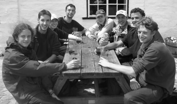
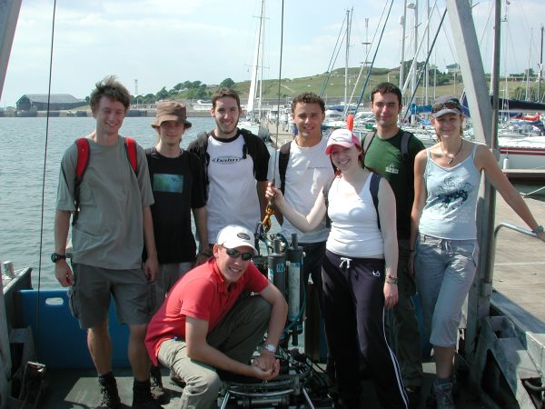
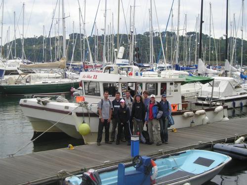
| Group 9 (clockwise from bottom left) Will Butler, Morvan Barnes, Elle Wolf, Simon King, Nikki Parker, Julian "Westcountry Bill" Schanze, Kelvin Reay and Alex Mortley. |
|
Area of work, detailling estuarine RIB and work on R.V. Bill Conway as well as Geophysical Surveying and Offshore Work on M.V. Bonito |
- Contents -
![]()
![]()
![]()
![]()
![]()
| Introduction |
|
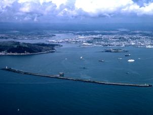
The marine areas subject to investigation during the Plymouth fieldcourse are the Tamar estuary, Plymouth Sound and the surrounding offshore waters. Situated on the south coast of England, the drowned river valley of the Tamar separates the two counties of Devon and Cornwall. Historically a major British port for trading and military affairs, the city of Plymouth has evolved accordingly, forcing the natural harbour to change in its style and purpose. The study area stretches from the offshore coastal waters, of 70m in depth, to the shallow upper reaches of the Tamar estuary. In the centre of the study area is Plymouth Sound which has a maximum width of 6km and a mouth that is 5km wide. Built in the early 19th century one of the key features, located in the centre of The Sound, is Plymouth Breakwater. The Tamar estuary is a mesotidal/macrotidal, partially mixed, flood dominant estuary. About 30km long, it has an average river discharge of 22m³s-¹ and a tidal range of 2.1m at neap tides and 4.7m at springs. By topography, the estuary type is classified as a ria (Dyer, 1997). Inthe estuary the Tamar merges with the rivers Tavy, Plym and Lynher. At the mouth of the river the freshwater is assisted past the constraints of Drake’s Island by the dredging of the channel. Here the channel moves around the eastern side of The Sound until it splits at the breakwater to create what are known as the Eastern and Western Channels. |
|
Objectives
|
| Bonito (Offshore) |
|
|
Met DataAir Temperature: 15°C Wind Direction & Speed: W/WSW 15km/h Cloud Cover & Precipitation: Partly cloudy, light rain Tides: High water: 1340GMT, 4.51m, Low water: 0720GMT, 1.93m & 1950GMT, 1.95m. |
|
Station |
Description |
|
One |
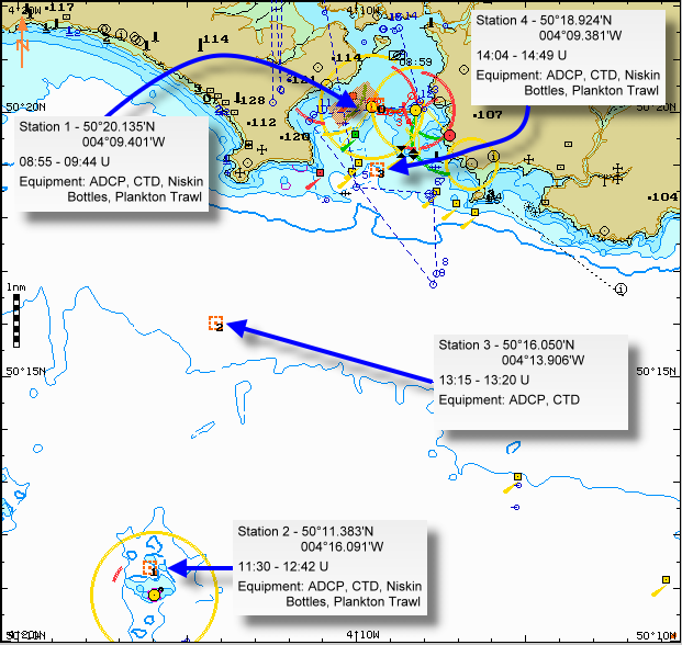
Position: 50° 20.135'N 004° 09.401'W (inside Breakwater) Date/Times: 01/07/2005, arrival 0855GMT, departure 0944GMT Conditions: showers, overcast, sea state slight Instruments: ADCP profile, CTD profile, surface plankton trawl & vertical plankton trawl |
|
Two |
Position: 50° 11.383'N 004° 16.091'W ( north of Eddystone Rocks) Date/Times: 01/07/2005, arrival 1130GMT, departure 1242GMT Conditions: showers, overcast, sea state rough Instruments: ADCP profile, CTD profile, vertical plankton trawl |
|
Three |
Position: 50° 16.021'N 004° 14.130'W (near L4) Date/Times: 01/07/2005, arrival 1315GMT, departure: 1320GMT
Instruments: ADCP profile, CTD Comments: Unfortunately due to failure of the CTD this station was abandoned. |
|
Four |
Position: 50° 18.924'N 004° 09.381'W (just outside Breakwater) Date/Times: 01/07/2005, arrival 1404GMT, departure 1449GMT Conditions: showers, overcast, sea state moderate Instruments Deployed: ADCP profile, CTD profile, vertical plankton trawl, secchi disk |
Biology
|
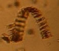 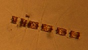 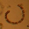
Examples of phytoplankton species seen in the lab. |
Zooplankton
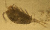
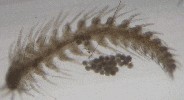
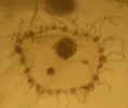
Dominant zooplankton species recovered from the vertical net trawls were; Hydrozoans, Echinoderm larvae, Siphonophores, Gastropod larvae, Copepods (calanoid/cyclopoid), Copepod nauplii andChaetognaths. Station 1 showed a dominance of hydrozoans (22%), station 2 a dominance of siphonophores (37%) and station 4 copepods (28%). Siphonophones were the only species present in large abundances at all 3 stations.
 Fig. 1: Station One phytoplankton composition
|
 Fig. 2: Station Two phytoplankton composition
|
 Fig. 3: Station Four phytoplankton composition
|
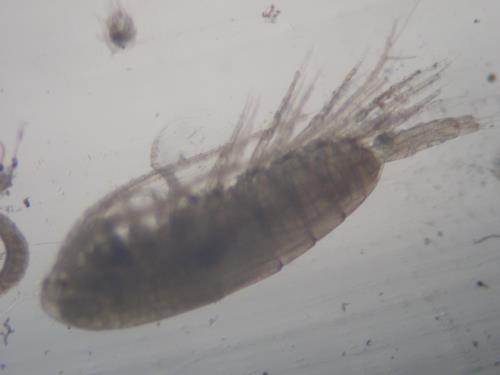
 Fig. 4: Zooplankton
|
Chemistry Oxygen At Station One the near surface is 111% saturated in oxygen and this decreases with depth to 42% and 39% at 5m and 13m respectively. In contrast Station Two shows a slight general increase of oxygen saturation with depth with a near surface value of 49% and ending at 55% at 30m. At Station Four the oxygen profile is similar to that at Station One but has near surface values of 54% with a slight but significant decrease with depth to 50% at 20m. In general it can be seen that Stations One and Four have a higher oxygen content in surface waters than at depth, as expected (Fig. 5). Nitrate The near-surface nitrate concentration (0.8m depth) at Station One was approximately 3.3μmolL-1; a sub-surface minimum of 2.6μmolL-1 was found at a 5m depth, before the concentrations increased again with depth to 3.8μmolL-1 at 13m. At Station Two, the nitrate concentration was found to decrease with depth from 2.4μmolL-1 at 4m depth to an approximate minimum of 1.5μmolL-1 at 19m. From here to 30m depth there was an increase to around 2μmolL-1. Station Four showed a steady decrease in nitrate concentration from 4.1μmolL-1 at 2m depth down to approximately 1.5μmolL-1 at 20m. All samples notably showed concentrations of nitrate much higher than would be expected for offshore waters (Fig. 6). Silicate The Station One silicate profile is similar to the phosphate and nitrate profiles with a gradual decrease in silicon from 1.84μmolL-1to 1.02μmolL-1between 2m to 14m respectively. At Station Two there is an immediate increase in the upper water column silicon levels followed by a significant reduction between 12m and 20m. This could be accounted for by the presence of diatoms directly above the seasonal thermocline or the possibility of contamination. A subsequent increase in silicon can be noted below 20m. Station Four however displays an expected significant increase in silicon from surface to 20m depth. These profiles therefore show evident signs of a general silicon increase with depth, combined with a significant silicon minima characteristic of sub-surface phytoplankton blooms (Fig. 7). Phosphate At Station One, the phosphate concentration showed a similar relationship with depth to nitrate, starting at 0.7μmolL-1 at 0.8m depth, decreasing to a minimum of 0.3μmolL-1 at 5m and increasing again to 0.7μmolL-1 at 13m. The phosphate concentration for 4m depth at Station Two is most probably an anomalous result, possibly due to contamination as it is unusually high. However, from 12m down, there is an increase in concentration and below 19m phosphate remains constant. At Station Four, a slight and possibly significant increase in concentration (of 0.2μmolL-1 up to 0.3μmolL-1) was observed from 2m down to 20m. The results are quite similar to expectations, as minima are located around the chlorophyll maxima, at 5m at Station One and 12m at the other two (Fig. 8). 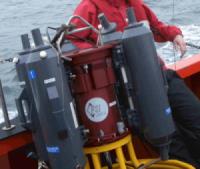 Physical Physical
In temperate North Atlantic waters, a seasonal thermocline forms in surface waters after the deep mixing of the previous thermocline during the winter months. This means that phytoplankton populations are no longer mixed over a depth greater than the euphotic zone, and that the mixing depth is shallower than the critical depth as defined by Sverdrup’s critical depth model. Station One, which is located landwards of the breakwater, shows influences of riverine input in the form of a layer of fresher, warmer water at the surface and heavier, more saline water at the bottom (Fig. 9). The riverine water brings with it also an additional input of nutrients, which means that the surface waters are not nutrient depleted, causing a shallow chlorophyll maximum. This is also caused by the high light attenuation of the water, which means limited light availability for phytoplankton growth at depths beyond the euphotic zone. The samples taken at Station Two show far less influence of estuarine input; the main seasonal thermocline occurs around 15-16m depth. A chlorophyll maximum at this depth indicates nutrient limitation in surface water. The light entering the water experiences less attenuation, with the euphotic zone reaching down to approximately 22m (Fig. 10). A Brunt-Vaisala frequency calculation shows values of 5/hr for the surface 5 metres, and 14/hr for the main thermocline. Below 15m, the frequency decreases to 6/hr (below 22m). This signifies a greater stratification than would be expected in the open ocean, which generally shows frequencies of 2-4/hr for the main thermocline. Station Three, located near station “L4”, shows similar properties to those observed at Station Two, namely a chlorophyll maximum linked with the seasonal thermocline at 14-16m depth (Fig. 11). Station Four shows a shallower thermocline around 10m depth, which coincides with the chlorophyll maximum at this depth (Fig. 12); this is, however, not as pronounced as the maxima observed at Stations Two and Three. Attempts were made, using the CTD data and the ADCP current data to calculate the Richardson number for each station. However, due to unuseable ADCP data (as a result of bad weather conditions) our calculations were largely unrealistic. For example, for station one a Richardson number of 132.8 was obtained, indicating a high degree of stratification. This can be compared to a value calculated using a nearby tidal diamond, which yields an excessively high value of 1174. This analysis is therefore not included.
|
|

|
| Not everyone enjoyed the day as much as Julian! |
ConclusionsThrough the course of this practical, a varying degree of thermal stratification was observed. As our distance from the breakwater increased (and the effects of estuarine mixing were minimized), the thermocline became more pronounced and was observed at a greater depth. In accordance with this, a chlorophyll maximum was observed at a depth slightly above that of the thermocline indicating a prominent offshore phytoplankton bloom. Being subject to significant estuarine influence, Station One does not display such trends and shows no observable thermocline or sub-surface chlorophyll maximum. Instead, influential riverine nutrient inputs promotes a near surface chlorophyll maximum. The extensive phytoplankton populations offshore result in the subsequent depletion of major nutrients such as nitrate, phosphate and in the case of diatoms, silicate. Phytoplankton composition was seen to vary only slightly between stations, however diatoms were the predominant phytoplankton group at each station and were almost exclusively dominant at depth. Dinoflagellates were at their most abundant in offshore surface waters, and a few other key species were also recorded. The dissolved oxygen profiles did not show such clear
results although it can be noted that a general decrease with depth was
interrupted for our most offshore stations possibly due to extensive mixing. |
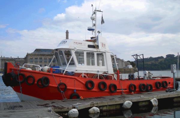
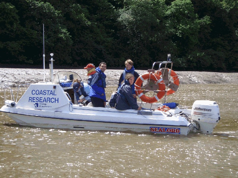
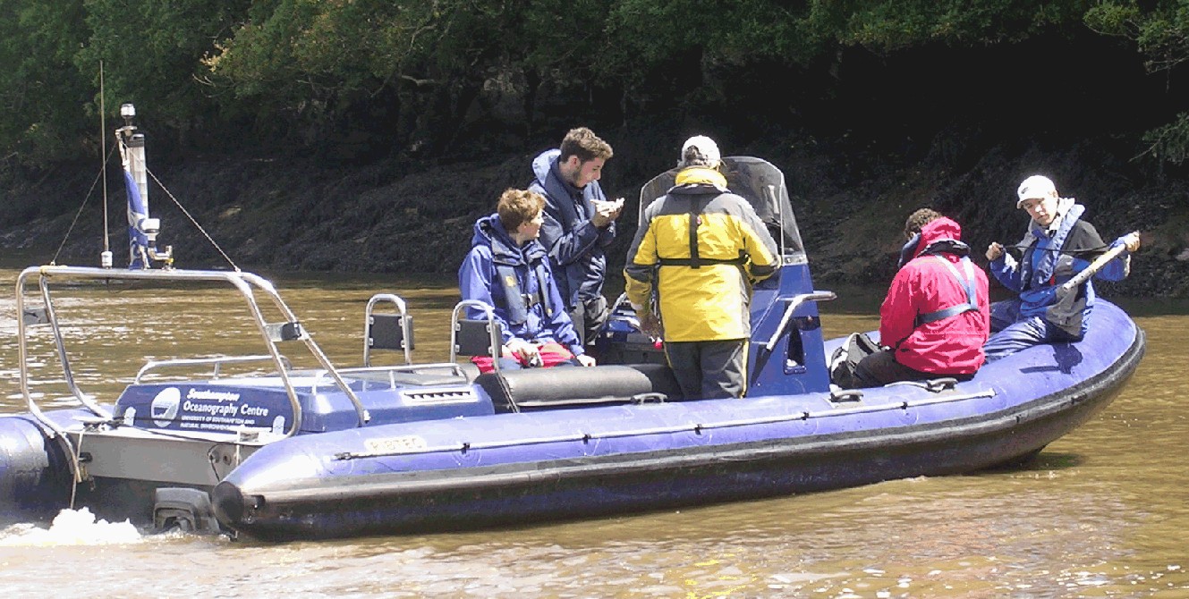
| Bill Conway (Lower Estuarine) |
|
 Group
aboard Bill Conway
Group
aboard Bill Conway
|
|
 Winch wench
|
Met DataAir Temperature: 21-27°C Wind Direction & Speed: E 9km/h Cloud Cover & Precipitation: clear Tides: High water; 0833GMT, 4.7m & 2003GMT, 4.9m. Low water; 1404GMT, 1.6m.
|
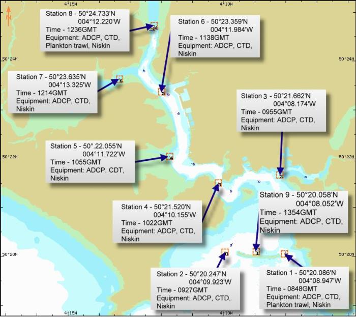
ResultsBiologyPhytoplanktonIn total 3 stations were sampled for phytoplankton composition. Of the target species monitored only diatom species were found, however there were discrepancies between stations. Station Eight, situated just South of the Tamar bridge and therefore the furthest up the estuary, showed the highest number of diatoms per litre of seawater (276000), and consisted predominantly of Chaetoceros sp. (85%), a species that was identified as characteristic of the upper estuary. Nonetheless 8 other species were found at this location. Station Four located at the “narrows” showed a slightly inferior number of diatoms per litre seawater (209000). Although once again the dominant species was found to be Chaetoceros sp., it only represented 36% of the total phytoplankton population. Other species also proved dominant such as Rhizosolenia delicatula and Rhizosolenia stolterfothii represented 26% and 19% respectively. Station One, situated East of the breakwater and the furthest down the estuary, showed significantly fewer total diatom cells (31000 per litre seawater). Chaetoceros in particular only represented 13% whereas the most dominant species was Rhizosolenia stolterfothii (32%). ZooplanktonTwo zooplankton trawls were conducted, one at station One (at the mouth of the estuary) and one around station Eight (further up the estuary). Station One exhibited a particularly high percentage of copepods (Fig. 13)(54%) and a notable 18% of siphonophores. On the other hand Station Eight displayed a slightly lower proportion of copepods (34%) and a significant proportion of carripede nauplii (29%) – none having been recorded for Station One. Siphonophores were also present in low abundance (13% of total). ChemistryOxygenDissolved Oxygen Saturation depends on both salinity and temperature. Due to surface mixing and primary productivity, the surface waters are supersaturated at all stations. Depending on the light attenuation, and consequently the euphotic depth, photosynthesis and respiration are the main controlling factors on dissolved oxygen saturation at depths between 5m and 30m in the estuary. Station one, located at the breakwater and taken during ebbing tides, shows almost no changes of saturated oxygen with depth, this is presumed to be due to strong mixing and a resulting breakdown of stratification at the narrows during the ebb tide. The euphotic zone at this station is estimated to be 16.7m by measure of a Secchi disc (factor *3 assumed), which means that net phytoplankton respiration should not be a major factor above depths of 10m. Stations 3-8 exhibit a clear decrease with depth, this can be attributed to the respiration at depth, with euphotic zones estimations of 13.4m (station 3), 12.9m (Station 4), 6.7m (Station 6) and 3.5m (Station 8). This can be seen in the rapid decrease of dissolved oxygen saturation at stations 6 and 8(Fig. 14). Returning to the breakwater at 1352 GMT for Station 9, the tide had almost reached its lowest state and was starting to become slack. In these more stratified conditions than Station 9, the dissolved oxygen saturation was found to be greater at 11.6m depth than in surface waters, which is presumed to be due to a high phytoplankton photosynthetic rate in these depths. The euphotic zone was estimated to be 15.1m by means of a Secchi disk measurement. NitrateSimilar to the findings from the upper estuary, nitrate showed a typically conservative behaviour, decreasing roughly linearly with salinity from a maximum of 11.3 μmol/L at the Tamar Bridge down to a minimum at the eastern side of the breakwater of 1.5 μmol/L. However the small scale surface salinity change along the lower estuary rendered interpretations difficult (Fig. 15). SilicateThe estuarine mixing diagram of salinity against silicate concentrations shows a steady decrease of silicate concentrations with increasing salinity. However, some of the data points were in excess of 10% variation around the theoretical dilution line. This would suggest non-conservative behaviour due to additions and removal of the silicate concentrations. For example, removal of silicate is indicated at the Lynher station. This removal is probably due to phytoplankton cells (diatoms) utilising the silicate during growth which is required for their cell wall. Addition of silicate concentrations are found at stations with greater riverine influence (Fig. 16). PhosphateThe lower estuarine phosphate mixing diagram however is somewhat different from its upper estuarine counterpart. Phosphate appears to show non-conservative properties and there is strong evidence of phosphate addition to the estuary, with all data falling above the theoretical dilution line. Station 3, at the Cattewater mouth displays particularly high phosphate concentrations (>0.5 µmol/L) possibly due to a nearby sewage outlet. There was not a consistent relationship between depth and phosphate concentrations showing evidence of estuarine mixing (Fig. 17). PhysicalAt Station One in the Eastern Channel around the breakwater,
a possible thermocline and halocline can be seen with some evidence of overnight
cooling to a depth of 4m. A chlorophyll maxima can also be seen at 10m depth (Fig.
18).
The ADCP profile at 0840 GMT showed a consistently low velocity of an average of
0.037m/s. There was no defined direction of current flow due to the state of the
tide being at high water slack. A frontal system was detected by a prominent scum line in the Hamoaze Shallows at 1042GMT. This was indicated in the backscatter profile at a definite horizontal change in backscatter which increased as the ADCP passed through the frontal system (Fig. 21). The confluence of the River Lynher
shows similar properties of temperature and salinity to the
Narrows profile with two clearly defined layers with the boundary at 4m.
However, the fluorescence appears to be significantly
higher in the mixed layer with fluorometer readings of
above 2.10 Volts (Fig. 22). The Brunt-Vaisala frequency at Station 1 was found to be 16/hr for the entire water column, while Station 7 showed greater stratification, with a Brunt-Vaisala frequency of 45/hr. This shows the greater stratification of the estuary compared to the offshore stratification, which was found to be 15/hr at the main thermoline at Offshore Station 2.
|


ConclusionsIt has been found that the abundance of phytoplankton species change from the Tamar Bridge to the breakwater. Diatoms generally decrease with salinity with the most dominant being Chaetoceros at 36% of total species present at Station Eight. With zooplankton, Copepods appear most dominant in the highest salinities at the Breakwater and less so further up in the estuary. In regards to dissolved oxygen, all surface samples at all stations are supersaturated and there is a general decrease with depth. Nitrate shows conservative behaviour and decreases in concentration with increasing salinity. Silicate appears to be non conservative but still decreases with increasing salinity. Phosphate is non conservative with a possible sewage outfall identified in the Station Three sample. There was also no consistent relationship between phosphate and depth indicating mixing. The physical structure is varied but shows some partial stratification at Station One (Breakwater) and strong mixing at Station Four (Narrows) with warm water overlying a mixed layer, progressing to haline stratification at Station Eight (Tamar Bridge). Current flows within the estuarine system have been shown to follow the tidal direction and indicate areas of strong mixing especially in the channalised regions around the Narrows and slightly to the North.
|
| RIBs (Upper Estuarine) |
|
|
Met DataAir Temperature: 14°C Wind Direction & Speed: W/WNW 13km/h Cloud Cover & Precipitation: Partly cloudy, light showers Tides: High water: 1634GMT, 4.0m. Low water: 1100GMT, 1.0m. |
Stations:
|
ResultsBiologyPhytoplanktonThe estuarine waters were almost exclusively dominated by diatoms, in particular colonies of Chaetoceros (Fig. 25), a centric chain forming species. The average number of cells per colony of Chaetoceros was 6.8 and this number did not vary significantly with salinity. In low salinity waters, Chaetoceros represented 100% of total cell abundance (salinity values 8 to 14). Overall, the number of phytoplankton cells per litre of water increased with increasing salinity; for example at salinity 8, 8000 Chaetoceros colonies were found compared to 100000 colonies found at salinity 26. As the salinity increased seawards down the estuary, other cell species were also found in low abundances, most notably the ciliate Mesodinium, which represented 24% of the total cell abundance at salinity 26. Various Rhizosolenia species were found exclusively at intermediate salinities and also the dinoflagellate Ceratium fusus (Fig. 24).
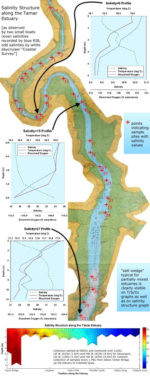
ZooplanktonOne zooplankton surface net sample was taken at salinity 7.86 in the Tamar Estuary (Position 50º 28.125N, 004º 13.960W). Analysis of this sample revealed that the zooplankton community at this location and time was dominated by copepods (94%). Other zooplankton species were also present in low abundances, Hydrozoans (2%), Polychaete larvae (1%), Mysids (1%) and Siphonophores (1%). The flooding tide showed a strong tidal flow of 642.7m³ of water through flow meter over the 6 minute deployment of the net. Therefore, copepod abundance was calculated at 16 organisms per 1m³ of seawater. ChemistryOxygenIn general the surface oxygen data shows an increase in percentage saturation with increasing salinity from 102.5% to 153.7%, however the oxygen minimum was obtained at a salinity of 12 with a rapid increase towards higher salinities. The data fluctuates heavily with an average range of ±10% but the data from the probe correlates well with the oxygen saturation of the water samples (Fig. 26). Data from the individual stations shows that oxygen saturation decreases with depth as would be expected but due to the varying depths of the channel, only surface saturations have been used for lateral comparisons. NitrateSurface nitrate concentrations showed a generally conservativebehaviour, when plotted against salinity on an estuarine mixing diagram. Near zero salinity, the nitrate concentration was the greatest recorded, at 173.5μmolL-1. With increasing salinity, nitrate decreases linearly in concentration to a minimum of 22.9μmolL-1 at 27 salinity. Data points at 10 and 18 salinity are anomalous indicating either contamination or inputs of nutrients into the estuarine system from external sources, such as sewage outfalls (Fig. 27). SilicateThe concentrations of silica demonstrate a non-conservative behaviour with respect to salinity change. Concentrations decrease by approximately 50μmolL-1 from a maximum of 68.0μmolL-1 at the riverine end of the estuary to 17.9μmolL-1 at a salinity of 27. There is an obvious removal process acting upon the dissolved silicate, with all data falling in an arc below the theoretical dilution line. The anomalous data from the nitrate and phosphate plots (indicative of contamination or nutrient inputs to the estuary) are not apparent on the silicate diagram (Fig. 28). PhosphateThe data for phosphate concentrations along the upper estuary are a lot less precise than those for nitrate. Like nitrate, there is a tendency for phosphate to decrease in concentration with increasing salinity, from 1.3μmolL-1 at a salinity of 1 down to 0.6μmolL-1 at the seaward end of the survey. In general, it would appear that phosphate has a non-conservative behaviour and is removed from this system, as most data fall below the theoretical dilution line (Fig. 29). Also similarly to nitrate, there are some possible nutrient inputs (potentially from Cargreen or nearby sewage outlets) or contamination at salinities of 10 and 18, as well as at 2 and 24 (which do not appear on the estuarine mixing diagram for nitrate). PhysicalAll observations refer to the observation period between 0905GMT downstream of the Tamar bridge (Salinity=27) until 1226GMT, downstream of Cotehele Quay (Salinity=0.4) on the 4-7-2005. The Tamar estuary is a partially mixed estuary, which means that despite some turbulent mixing, there are still signs of stratification. This stratification occurs in form of haline stratification in the lower reaches of the estuary, such as around the Tamar bridge area, in which salinity changes from 27-32 were found from surface to the bottom. Another factor aiding stratification is the temperature, which is highest at the surface and lowest at the bottom (Fig. 30). The haline stratification was most pronounced in the observed area at intermediate salinities of 10-20, in the case of Salinity=15, this changes from 15 at the surface to 24 at the bottom. The upper reaches of the estuary are more mixed, which is indicated by the secchi disc depths, which are decreasing from 1.85m at Salinity=27 to approximately 0.2m at Salinity=4-6. Since the secchi disk depth at salinities lower than 4 starts to increase again, it is presumed that the turbidity maximum occurs at salinities 3-7. |
ConclusionsAnalysis of the data obtained from the rib practical showed almost exclusive dominance of diatoms cells within the phytoplankton assemblage with increased cell abundance with increasing salinity. This correlates with increasing dissolved oxygen, decreasing nitrate, silicate (a continuous removal process was occurring) and phosphate concentrations with the increasing diatom populations utilizing these nutrients and producing dissolved oxygen by the process of photosynthesis. Addition of nitrate concentrations has been identified at samples with salinities of 10 and 18. These may be due to contamination of the samples, however, external additions of nitrate may also be due to the station with a salinity of 18 being located close to the town of Cargreen and the station at salinity 10 was enclosed within a frontal system (identified by an area of small rippling waves). Vertical depths profiles show a prominent presence of a halocline occurring from the Tamar Bridge to salinity of 1. As with all estuaries, characteristics of the estuary are consistently changing with the state of the tide, seasons, atmospheric and anthropogenic influxes. Therefore, data obtained and subsequently analysed within this investigation can only describe the biological, chemical and physical characteristics of the Tamar estuary at the sampling stations for that particular day and time. Sampling within the Plymouth Sound is the next progressive step, in particular to establish the location of the formation of the halocline.
|
| Geophysics (Natwest II) & Geofield |
Geophysical Survey
|
Met DataAir Temperature: 17°C Wind Direction & Speed: N/NNW 10km/h Cloud Cover & Precipitation: Partly/mostly cloudy Tides: High water: 0641GMT, 4.1m & 1851GMT, 5.1m. Low water: 1300GMT, 1.3m. |
Wreck sites
Ship |
Date |
Time |
Position |
| Scylla | 08/07/2005 | 0912GMT - 0948GMT | 50° 19.7'N, 004° 15.2'W |
| James Egan Layne | 08/07/2005 | 0950GMT - 1033GMT | 50° 19.6'N, 004° 14.8'W |
|
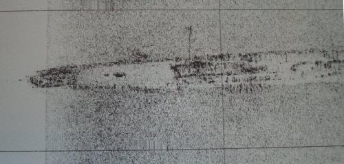
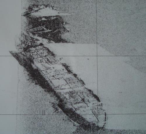
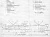
The dimensions of both vessels can be roughly calculated through geometric correction of the sonar print outs. The Scylla (Fig. 31)is a British naval frigate that was sunk in 2004 as an artificial reef. From our measurements it has been found that the Scylla is approximately 10m above the seabed, (16m at the highest point), 100m long and 11m wide. In contrast the other wreck in Whitsand Bay is of the James Egan Layne (Fig. 32), a liberty cargo vessel that sank during the Second World War. This ship has approximate dimensions of 9m above the seabed (averaged out from 3 separate images), 100m long and 21m wide from our calculations. External sources (Fig. 33, website: submerged.co.uk)confirmed the dimensions as height 11.3m, length 120m and width 17.7m and shows our methods are reasonably accurate bearing in mind the resolution of the surveys. The contrast in sedimentary features between the sediments surrounding both vessels can clearly be seen with heavy scouring around the James Egan Layne. Seafloor sediment survey
A location directly west of Rame Head provides an opportunity to survey the shallow coastal shelf. From the navigational software the initial master line, with start point 50º 20’.5 N 004º 16’.5 W and end point 50º 20’.5 N 004º 20’.5 W, was established. Five further lines were applied to the left of the master at 100m intervals. After commencing the survey it was decided that the track should be shortened, with westward tracks commencing at 50º 20’.5 N 004º 17’.5 W . See chart. The sonar traces provided an oblique picture of the seafloor. Correcting the distortion enabled a geological map to be drawn on a plot designed by ‘Surfer’. Four categories were determined; fine sediment, coarse sediment, coarse sediment with ripples and bedrock. Fine sediment and bedrock dominates the chosen region from west to east respectively. Areas of coarser sediment are located nearer the shore. Ripple patterns have been identified from the sonar trace. An area of coarse sediment ripples is located in the north-east corner of the map (link to map). The ripples are mostly parallel with some bifurcating.
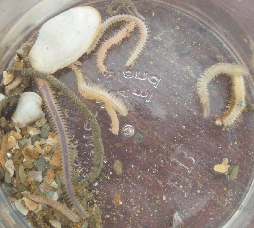
Grab one contained predominately fine sand and sediment. Some coarser sediment with many shells and shale was observed in the upper sieve. Also one Polychaete worm was identified. Grab two consisted largely of very fine sand and mud with the presence of three Polychaete worms(Fig. 34). Many rocks and a few broken shells were observed in the 2mm sieve. Lots of finer shale and shells between 1 and 2mm. Detailed sediment matrix and evidence of biological activity nearer the shore.
|
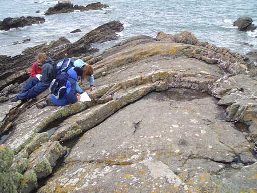
Geological FieldworkAimTo introduce basic land-based field survey techniques of location and use of compass-clinometer to record structural data. This structural data includes dip and strike (right hand rule) of beds and geometry of folds, faults and fractures. This data is then used in the interpretation of the geophysical survey findings.
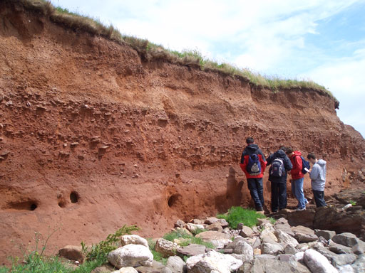
Structural Geological SettingThe district is dominated by Devonian bed forms which have been extensively altered by regional geological forces. A asymmetrical, parasitic recumbent fold structure can be seen on the coastal exposure at Renney Point (SX492488) as shown on Fig. 35. The beds show a general dip to SE of the southern fold limbs with a fold hinge axis to the SW and plunge of ~16°(Fig. 36). Extensive faulting has also occurred in the region with a clearly visible strike/slip dextral fault with a NW-SE orientation (Fig. 37). The offset is estimated at 15m and a variety of fractures can be seen in the surrounding rock with many having a similar orientation to the fault. Faults generally occur along one of two diagonal planes within a block. Fractures normally occur on the opposing plane to the fault (Fig. 37). Other fractures may be seen in other orientations along with tension cracks due to other processes and the complexity of the geology in the district. Sedimentary featuresA sedimentary log (Fig. 38) of the cliff section above the basal Devonian bed forms shows evidence of a terrestrial environment with mainly colluvium facies present (Fig. 39). The basal unit of the sequence (A1) is a debrite deposited from a debris flow which suggests a high energy environment but a low degree of transport duration due to the angularity of the clasts within the unit. The unit was also deposited rapidly as no sorting can be seen within the deposit. As the sequence gets younger, the units change from being clast supported to matrix supported conglomerates interbedded with medium sands (A3) and red clays (A2, A4). These units tend to indicate a low energy environment with slow deposition rates. The matrix supported conglomerate shows orientation of clasts in a lateral plane and may have been caused by loading structures or by slower deposition. Unit A3 shows some lenticulation while the other units demonstrate lateral continuation. This suggests channelisation within the deposit and may be evidence for a palaeo-braided river channel. The red colour present in the A units is caused by the oxidation of iron possibly indicating an oxygen rich environment during the period of deposition (further evidence for terrestrial environment) or ground water leaching of iron minerals. At the top of the sequence there is an abrupt change in colour of the deposits and marine shell fragments can be found within the sandier B1 unit. This unit represents a shallow marine environment and therefore infers that regional sea level has risen and changed the environment from terrestrial to marine.
|
Geophysical and Geological ConclusionsThe surveys of both the marine and terrestrial geological environments have provided an extensive data set encompassing a range of initial aims from imaging of the wreck sites to seafloor sediment surveys and structural analysis of the Devonian Limestones. The Limestone bed rock has shown that the district has undergone extensive structural reworking with evidence of folding and strike/slip faulting. The sedimentary analysis of the tertiary cliff section describes the change from a terrestrial to shallow marine environment. The structures within part of this section also provide evidence for palaeo-river channels. The recent seafloor sediments are patchy in nature and mainly consist of fine and coarse grain sediments, some with ripple structures, all lying on the limestone bedrock. Grab samples confirm these observations and give an indication to the main benthic fauna present in the area. The data set also provides an opportunity for an applied use of geophysics to remotely monitor the wrecks of the HMS Scylla and James Egan Layne. These methods have allowed us to briefly study some of the geological history of the Plymouth region in comparison with the present day oceanographic data. |
ReferencesParsons T. R. Maita Y. and Lalli C. (1984) “ A manual of chemical and biological methods for seawater analysis” 173 p. Pergamon. Grasshoff, K., K. Kremling, and M. Ehrhardt. (1999). Methods of seawater analysis. 3rd ed. Wiley-VCH. Johnson K. and Petty R.L.(1983) “Determination of nitrate and nitrite in seawater by flow injection analysis” Limnology and Oceanography 28 1260-1266. Miller, C.B. (2004). Biological Oceanography. Blackwell Publishing, Oxford. Dyer, K.R. (1997). Estuaries: A Physical Introduction. 2nd ed. John Wiley and Sons Ltd, Chichester. Websites |
And just for fun...
Which creature of the sea are you? Find out by following this link!